Abstract

We generalize the orthogonally transitive (OT) $G_{2}$ spike solution to the non-OT $G_{2}$ case. This is achieved by applying Geroch’s transformation on a Kasner seed. The new solution contains two more parameters than the OT $G_{2}$ spike solution. Unlike the OT $G_{2}$ spike solution, the new solution always resolves its spike.

[PACS: 98.80.Jk, 04.20.-q, 04.20.Jb]

1 Introduction

According to general relativity, in the asymptotic regime near spacelike singularities, a spacetime would oscillate between Kasner states. The BKL conjectures [art:LK63, art:BKL1970, art:BKL1982] hold except where and when spikes occur [art:BergerMoncrief1993, art:GarfinkleWeaver2003]. Spikes are a recurring inhomogeneous phenomenon in which the fabric of spacetime temporarily develops a spiky structure as the spacetime oscillates between Kasner states. See the introduction section of [art:HeinzleUgglaLim2012] for a comprehensive background.

Previously in [art:Lim2008] the orthogonally transitive (OT) $G_{2}$ spike solution, which is important in describing the recurring spike oscillation, was generated by applying the Rendall-Weaver transformation [art:RendallWeaver2001] on a Kasner seed solution. The solution is unsatisfactory, however, in that it contains permanent spikes, and there is a debate whether permanent spike are actually unresolved spike transitions in the oscillatory regime or are really permanent. In other words, would the yet undiscovered non-OT $G_{2}$ spike solution contain permanent spikes? The proponents for permanent spikes argue that the spatial derivative terms of a permanent spike are negligible, and hence the spike stays permanent [art:Garfinkle2007]. The opponents base their argument on numerical evidence that the permanent spike is mapped by an $R_{1}$ frame transition to a regime where the spatial derivative terms are not neglibigle, which allows the spike to resolve [art:HeinzleUgglaLim2012]. To settle the debate, we need to find the non-OT $G_{2}$ spike solution. It was found that Geroch’s transformation [art:Geroch1971, art:Geroch1972] would generate the desired solution, which always resolves its spike. The next section describes the generation process.

2 Generating the solution

For our purpose, we express a metric $g_{ab}$ using the Iwasawa frame [art:HeinzleUgglaRohr2009], as follows. Indicies $0,1,2,3$ corresponds to coordinates $\tau,x,y,z$. Assume zero vorticity (zero shift). The metric components in terms of $b$’s and $n$’s are given by

$$g_{00} =-N^{2}$$ (1)

$$g_{11} =e^{-2b_{1}},\quad g_{12}=e^{-2b_{1}}n_{1},\quad g_{13}=e^{-2b_{1}}n_{2}$$ (2)

$$g_{22} =e^{-2b_{2}}+e^{-2b_{1}}n_{1}^{2},\quad g_{23}=e^{-2b_{1}}n_{1}n_{2}+e^{-2b_{2}}n_{3}$$ (3)

$$g_{33} =e^{-2b_{3}}+e^{-2b_{1}}n_{2}^{2}+e^{-2b_{2}}n_{3}^{2}.$$ (4)

One advantage of the Iwasawasa frame is that the determinant of the metric is given by

$$\det g_{ab}=-N^{2}e^{-2b_{1}-2b_{2}-2b_{3}}.$$ (5)

A pedagogical starting point is the Kasner solution with the following parametrization:

$$b_{1}=\frac{1}{4}(w^{2}-1)\tau,\quad b_{2}=\frac{1}{2}(w+1)\tau,\quad b_{3}=-\frac{1}{2}(w-1)\tau,\quad N^{2}={\rm e}^{-2b_{1}-2b_{2}-2b_{3}}={\rm e}^{-\frac{1}{2}(w^{2}+3)\tau},$$ (6)

and $n_{1}=n_{2}=n_{3}=0$. We shall use a linear combination of all three Killing vector fields (KVFs)

$$a_{1}\partial_{x}+a_{2}\partial_{y}+a_{3}\partial_{z}.$$ (7)

as the KVF in Geroch’s transformation, so that the transformation generates the most general metric possible from the given seed.

2.1 Change of coordinates

To simplify the KVF before applying Geroch’s transformation, make the coordinate change

$$x=X+n_{10}Y+n_{20}Z,\quad y=Y+n_{30}Z,\quad z=Z$$ (8)

where $n_{10}$, $n_{20}$, $n_{30}$ are constants. Then the metric parameters $b_{1}$, $b_{2}$, $b_{3}$ and $N$ are unchanged but $n_{1}=n_{10}$, $n_{2}=n_{20}$, $n_{3}=n_{30}$ are now constants instead of zero. The KVF becomes

$$(a_{3}(n_{10}n_{30}-n_{20})-a_{2}n_{10}+a_{1})\partial_{X}+(a_{2}-a_{3}n_{30})\partial_{Y}+a_{3}\partial_{Z}.$$ (9)

We cannot set the $Z$ component to zero, but we can set the $X$ and $Y$ components to zero, leading to

$$n_{30}=\frac{a_{2}}{a_{3}},\quad n_{10}=\frac{a_{1}}{a_{3}}.$$ (10)

Without loss of generality, we set $a_{3}=1$, and so $n_{30}=a_{2}$ and $n_{10}=a_{1}$. $n_{20}$ remains free. We will see later that it can be used to eliminate any $y$-dependence.

To make transparent the effect of Geroch’s transformation on the $b$’s (see (34)–(37) below), it is best to adapt the KVF to $\partial_{x}$. So we make another coordinate change to swap $X$ and $Z$:

$$X=\tilde{z},\quad Y=\tilde{y},\quad Z=\tilde{x},$$ (11)

which in effect introduces frame rotations to the Kasner solution. The Kasner solution now has

$$N^{2} ={\rm e}^{-\frac{1}{2}(w^{2}+3)\tau}$$ (12)

$${\rm e}^{-2b_{1}} ={\rm e}^{(w-1)\tau}+n_{20}^{2}{\rm e}^{-\frac{1}{2}(w^{2}-1)\tau}+n_{30}^{2}{\rm e}^{-(w+1)\tau}$$ (13)

$${\rm e}^{-2b_{2}} =\frac{\mathcal{A}^{2}}{{\rm e}^{-2b_{1}}}$$ (14)

$${\rm e}^{-2b_{3}} ={\rm e}^{-\frac{1}{2}(w^{2}+3)\tau}\mathcal{A}^{-2}$$ (15)

$$n_{1} =\frac{n_{30}{\rm e}^{-(w-1)\tau}+n_{10}n_{20}{\rm e}^{-\frac{1}{2}(w^{2}-1)\tau}}{{\rm e}^{-2b_{1}}}$$ (16)

$$n_{2} =\frac{n_{20}{\rm e}^{-\frac{1}{2}(w^{2}-1)\tau}}{{\rm e}^{-2b_{1}}}$$ (17)

$$n_{3} ={\rm e}^{-\frac{1}{2}(w^{2}-1)\tau}\mathcal{A}^{-2}\left[n_{30}(n_{10}n_{30}-n_{20}){\rm e}^{-(w+1)\tau}+n_{10}{\rm e}^{(w-1)\tau}\right],$$ (18)

where

$$\mathcal{A}^{2} =(n_{10}n_{30}-n_{20})^{2}{\rm e}^{-\frac{1}{2}(w+1)^{2}\tau}+n_{10}^{2}{\rm e}^{-\frac{1}{2}(w-1)^{2}\tau}+{\rm e}^{-2\tau}.$$ (19)

Effectively, we are applying Geroch’s transformation to the seed solution (12)–(18), using the KVF $\partial_{\tilde{x}}$. We shall now drop the tilde from the coordinates.

2.2 Applying Geroch’s transformation

Applying Geroch’s transformation using a KVF $\xi_{a}$ involves the following steps. First compute

$$\lambda=\xi^{a}\xi_{a}$$ (20)

and integrate the equation

$$\nabla_{a}\omega=\varepsilon_{abcd}\xi^{b}\nabla^{c}\xi^{d}$$ (21)

for the general solution for $\omega$. $\omega$ is determined up to an additive constant $\omega_{0}$. In our case we get

$$\lambda={\rm e}^{-2b_{1}}={\rm e}^{(w-1)\tau}+{\rm e}^{-\frac{1}{2}(w^{2}-1)\tau}n_{20}^{2}+{\rm e}^{-(w+1)\tau}n_{30}^{2},\quad\omega=2wn_{30}z-Ky+\omega_{0},$$ (22)

where the constant $K$ is given by

$$K=\frac{1}{2}(w-1)(w+3)n_{20}-2wn_{10}n_{30}.$$ (23)

We could absorb $\omega_{0}$ by a translation in the $z$ direction if $wn_{30}\neq 0$, but we shall keep $\omega_{0}$ for the case $wn_{30}=0$.

The next step involves finding a particular solution for $\alpha_{a}$ and $\beta_{a}$:

$$\nabla_{[a}\alpha_{b]} =\frac{1}{2}\varepsilon_{abcd}\nabla^{c}\xi^{d},\quad\xi^{a}\alpha_{a}=\omega,$$ (24)

$$\nabla_{[a}\beta_{b]} =2\lambda\nabla_{a}\xi_{b}+\omega\varepsilon_{abcd}\nabla^{c}\xi^{d},\quad\xi^{a}\beta_{a}=\omega^{2}+\lambda^{2}-1.$$ (25)

Without loss of generality, we choose $\theta=\frac{\pi}{2}$ in Geroch’s transformation, so $\alpha_{a}$ is not needed in $\eta_{a}$ below. We assume that $\beta_{a}$ has zero $\tau$-component. Its other components are

$$\beta_{1} =\omega^{2}+\lambda^{2}-1$$ (26)

$$\beta_{2} =n_{10}n_{20}^{3}{\rm e}^{-(w^{2}-1)\tau}+\left[2\frac{w-1}{w+1}n_{10}n_{20}n_{30}^{2}+\frac{4}{w+1}n_{20}^{2}n_{30}\right]{\rm e}^{-\frac{1}{2}(w+1)^{2}\tau}$$

$$\quad+2\frac{w+1}{w-1}n_{10}n_{20}{\rm e}^{-\frac{1}{2}(w-1)^{2}\tau}+(w+1)n_{30}{\rm e}^{-2\tau}+n_{30}^{3}{\rm e}^{-2(w+1)\tau}+F_{2}(y,z)$$ (27)

$$\beta_{3} =n_{20}^{3}{\rm e}^{-(w^{2}-1)\tau}+2n_{20}n_{30}^{2}\frac{w-1}{w+1}{\rm e}^{-\frac{1}{2}(w+1)^{2}\tau}+2n_{20}\frac{w+1}{w-1}{\rm e}^{-\frac{1}{2}(w-1)^{2}\tau}+F_{3}(y,z)$$ (28)

where $F_{2}(y,z)$ and $F_{3}(y,z)$ satisfy the constraint equation

$$-\partial_{z}F_{2}+\partial_{y}F_{3}+2(w-1)\omega=0.$$ (29)

For our purpose, we want $F_{3}$ to be as simple as possible, so we choose

$$F_{3}=0,\quad F_{2}=\int 2(w-1)\omega{\rm d}z=2w(w-1)n_{30}z^{2}-2(w-1)Kyz+2(w-1)\omega_{0}z.$$ (30)

The last step constructs the new metric. Define $\tilde{\lambda}$ and $\eta_{a}$ as

$$\frac{\lambda}{\tilde{\lambda}} =(\cos\theta-\omega\sin\theta)^{2}+\lambda^{2}\sin^{2}\theta,$$ (31)

$$\eta_{a} =\tilde{\lambda}^{-1}\xi_{a}+2\alpha_{a}\cos\theta\sin\theta-\beta_{a}\sin^{2}\theta.$$ (32)

The new metric is given by

$$\tilde{g}_{ab}=\frac{\lambda}{\tilde{\lambda}}(g_{ab}-\lambda^{-1}\xi_{a}\xi_{b})+\tilde{\lambda}\eta_{a}\eta_{b}.$$ (33)

In our case $\tilde{g}_{ab}$ is given by the metric parameters

$$\tilde{N}^{2} =N^{2}(\omega^{2}+\lambda^{2})$$ (34)

$${\rm e}^{-2\tilde{b}_{1}} =\frac{{\rm e}^{-2b_{1}}}{\omega^{2}+\lambda^{2}}$$ (35)

$${\rm e}^{-2\tilde{b}_{2}} ={\rm e}^{-2b_{2}}(\omega^{2}+\lambda^{2})$$ (36)

$${\rm e}^{-2\tilde{b}_{3}} ={\rm e}^{-2b_{3}}(\omega^{2}+\lambda^{2})$$ (37)

$$\tilde{n}_{1} =-2w(w-1)n_{30}z^{2}+2(w-1)Kyz-2(w-1)\omega_{0}z+\frac{\omega^{2}}{\lambda}(n_{30}{\rm e}^{-(w+1)\tau}+n_{10}n_{20}{\rm e}^{-\frac{1}{2}(w^{2}-1)\tau})$$

$$\quad-\left[n_{30}w{\rm e}^{-2\tau}+\frac{w+3}{w-1}n_{10}n_{20}{\rm e}^{-\frac{1}{2}(w-1)^{2}\tau}+\frac{w-3}{w+1}n_{20}n_{30}(n_{10}n_{30}-n_{20}){\rm e}^{-\frac{1}{2}(w+1)^{2}\tau}\right]$$ (38)

$$\tilde{n}_{2} =n_{20}{\rm e}^{-\frac{1}{2}(w^{2}-1)\tau}\left[-\frac{w+3}{w-1}{\rm e}^{(w-1)\tau}-n_{30}^{2}\frac{w-3}{w+1}{\rm e}^{-(w+1)\tau}+\frac{\omega^{2}}{\lambda}\right]$$ (39)

$$\tilde{n}_{3} =\mathcal{A}^{-2}\left[n_{10}{\rm e}^{-\frac{1}{2}(w-1)^{2}\tau}+n_{30}(n_{10}n_{30}-n_{20}){\rm e}^{-\frac{1}{2}(w+1)^{2}\tau}\right],$$ (40)

and $\mathcal{A}$, given by (19), is the area density [art:vEUW2002] of the $G_{2}$ orbits. Note that the $w=\pm 1$ cases would have to be computed separately, which we shall leave to future work. The new solution admits two commuting KVFs:

$$\partial_{x},\quad[-(w-1)K^{2}y^{2}+2(w-1)K\omega_{0}y]\partial_{x}+2wn_{30}\partial_{y}+K\partial_{z}.$$ (41)

Their $G_{2}$ action is non-OT, unless $n_{10}=n_{20}=0$. The solution is also the first non-OT Abelian $G_{2}$ explicit solution found.

In the next section we shall focus on the case where $K=0$, or equivalently, where

$$n_{20}=\frac{4w}{(w-1)(w+3)}n_{10}n_{30},$$ (42)

which turns off the $R_{2}$ frame transition (which is shown to be asymptotically suppressed in [art:HeinzleUgglaRohr2009]), and eliminates the $y$-dependence. Setting (42) in the rotated Kasner solution (12)–(18) also turns off the $R_{2}$ frame transition there, giving the explicit solution that describes the double frame transition $\mathcal{T}_{R_{3}R_{1}}$ in [art:HeinzleUgglaRohr2009]. The mixed frame/curvature transition $\mathcal{T}_{N_{1}R_{1}}$ in [art:HeinzleUgglaRohr2009] is described by the metric $\tilde{g}_{ab}$ with $n_{20}=n_{30}=0$. Both the double frame transition and the mixed frame/curvature transition are encountered in the exceptional Bianchi type VI${}_{-1/9}^{*}$ cosmologies [art:Hewittetal2003].

Setting $n_{10}=n_{20}=0$ yields the OT $G_{2}$ spike solution in [art:Lim2008]. To adapt the solutions in [art:Lim2008] to the Iwasawa frame here, let

$$b_{1}=-\frac{1}{2}(P(\tau,z)-\tau),\quad b_{2}=\frac{1}{2}(P(\tau,z)+\tau),\quad b_{3}=-\frac{1}{4}(\lambda(\tau,z)+\tau),\quad n_{1}=-Q(\tau,z),\quad n_{2}=n_{3}=0,$$ (43)

where $x$-dependence in [art:Lim2008] becomes $z$-dependence here, and set $w$ to $-w$, $\lambda_{2}=\ln 16$, $Q_{0}=1$, $Q_{2}=0$ there, and set $n_{30}=1$, $\omega_{0}=0$ here. As pointed out in [art:Limetal2009] and [art:Binietal2009], the factor 4 in Equation (34) of [art:Lim2008] should not be there.

3 The dynamics of the solution

To describe the dynamics of the non-OT spike solution, we shall plot the state space orbit projected onto the Hubble-normalized $(\Sigma_{+},\Sigma_{-})$ plane, as done in [art:Lim2008]. The formulas are

$$\Sigma_{+} =-1+\frac{1}{4}\mathcal{N}^{-1}\partial_{\tau}(\mathcal{A}^{2})$$ (44)

$$\Sigma_{-} =\frac{1}{2\sqrt{3}}\mathcal{N}^{-1}\partial_{\tau}(\tilde{b}_{2}-\tilde{b}_{1})$$ (45)

$$\mathcal{N} =\frac{1}{6}\left[\frac{\partial_{\tau}(\lambda^{2})}{\omega^{2}+\lambda^{2}}+\partial_{\tau}\ln(N^{2})\right]$$ (46)

[art:HeinzleUgglaRohr2009] uses a different orientation, where their $(\Sigma_{+},\Sigma_{-})$ are given by

$$\Sigma_{+} =-\frac{1}{2}(\Sigma_{+}+\sqrt{3}\Sigma_{-})$$ (47)

$$\Sigma_{-} =-\frac{1}{2}(\sqrt{3}\Sigma_{+}-\Sigma_{-})$$ (48)

The non-OT spike solution (with $K=0$, $\omega_{0}=0$) goes from a Kasner state with $2<w<3$, through a few intermediate Kasner states, and arrives at the final Kasner state with $w<-1$. The transitions are composed of spike transitions and $R_{1}$ frame transitions. The non-OT spike solution always resolves its spike, unlike the OT spike solution with $|w|<1$, which has a permanent spike.

For a typical Kasner source with $2<w<3$, there are six non-OT spike solutions, some of which are equivalent, that start there. For example, non-OT spike solutions with $|w|=\tfrac{1}{3},\ 2,\ 5$ all start at $w_{\text{source}}=\frac{7}{3}$. From there, however, there are two extreme alternative spike orbits. The first alternative is to form a “permanent” spike, followed by an $R_{1}$ transition, and lastly to resolve the spike. This was described in [art:HeinzleUgglaLim2012] as the joint spike transition. This alternative is more commonly encountered (assuming that permanent spikes are more commonly encountered than no-spike at the end of a Kasner era). The second alternative is to undergo an $R_{1}$ transition first, followed by a transient spike transition, and finish with another $R_{1}$ transition. By varying $n_{1}$ and $n_{3}$, one can get orbits that are close to one extreme alternative or the other, or some indistinct mix.

The sequence of $w$-value of the Kasner states for the spike orbit is given below. For non-OT spike solution with $|w|>3$, the first and second alternatives are

$$\frac{3|w|-1}{1+|w|},\ \frac{5+|w|}{1+|w|},\ 2+|w|,\ 2-|w|$$ (49)

$$\frac{3|w|-1}{1+|w|},\ \frac{3|w|+1}{|w|-1},\ \frac{|w|-5}{|w|-1},\ 2-|w|$$ (50)

For $1<|w|<3$, the first and second alternatives are

$$\frac{5+|w|}{1+|w|},\ \frac{3|w|-1}{1+|w|},\ \frac{3|w|+1}{|w|-1},\frac{5-|w|}{1-|w|}$$ (51)

$$\frac{5+|w|}{1+|w|},\ 2+|w|,\ 2-|w|,\frac{5-|w|}{1-|w|}$$ (52)

For $|w|<1$, the first and second alternatives are

$$\frac{5+|w|}{1+|w|},\ \frac{3|w|-1}{1+|w|},\ \frac{3|w|+1}{|w|-1},\frac{5-|w|}{1-|w|}$$ (53)

$$\frac{5+|w|}{1+|w|},\ 2+|w|,\ 2-|w|,\frac{5-|w|}{1-|w|}$$ (54)

For $|w|<1$, the first and second alternatives are

$$2+|w|,\ 2-|w|,\ \frac{5-|w|}{1-|w|},\ \frac{3|w|+1}{|w|-1}$$ (55)

$$2+|w|,\ \frac{5+|w|}{1+|w|},\ \frac{3|w|-1}{1+|w|},\ \frac{3|w|+1}{|w|-1}$$ (56)

For example, for $|w|=\tfrac{1}{3},\ 2,\ 5$, the first alternative is $\frac{7}{3},\ \frac{5}{3},\ 7,\ -3$ and the second alternative is $\frac{7}{3},\ 4,\ 0,\ -3$. See Figure 1.

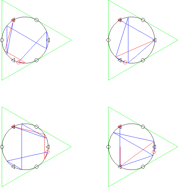
Figure 1: Alternative spike orbits for $w=5$. Top row is the orientation used in [art:Lim2008], bottom row is the orientation used in [art:HeinzleUgglaRohr2009]. Left column is the first alternative orbit, right column is the second alternative. Spike orbits ($z=0$) are in red, faraway orbits ($z=10^{12}$) in blue. Left column is generated with $n_{10}=10^{-3}$, $n_{30}=1$, right column with $n_{10}=10^{9}$, $n_{30}=10^{-9}$. A red circle marks the start of the orbits, a red star marks the end.

4 Summary

In this paper, we went through the steps of generating the non-OT $G_{2}$ spike solution, and illustrated its state space orbits for the case $K=0$, which show two extreme alternative orbits. More importantly, the non-OT $G_{2}$ spike solution always resolves its spikes, in contrast to its OT $G_{2}$ special case which produces an unresolved permanent spike for some parameter values. The non-OT $G_{2}$ spike solution shows that, in the oscillatory regime near spacelike singularities, unresolved permanent spikes are artefacts of restricting oneself to the OT $G_{2}$ case, and that spikes are resolved in the more general non-OT $G_{2}$ case. Therefore spikes are expected to recur in the oscillatory regime rather than to become permanent spikes. We also obtained explicit solutions describing the double frame transition and the mixed frame/curvature transition in [art:HeinzleUgglaRohr2009]. We leave the further analysis of the non-OT $G_{2}$ spike solution to future work.