Searching Heavier Higgs Boson via Di-Higgs Production at LHC Run-2

Abstract

The discovery of a light Higgs particle $\,h^{0}$ (125 GeV)  opens up new prospect for searching heavier Higgs boson(s) at the LHC Run-2, which will unambiguously point to new physics beyond the standard model (SM). We study the detection of a heavier neutral Higgs boson $\,H^{0}$ via di-Higgs production channel at the LHC (14 TeV), $\,H^{0}\!\!\rightarrow\!h^{0}h^{0}\!\!\rightarrow\!WW^{*}\gamma\gamma$ .  This directly probes the $\,Hhh\,$ cubic Higgs interaction, which exists in most extensions of the SM Higgs sector. For the decay products of final states $\,WW^{*}$,  we include both pure leptonic mode $\,WW^{*}\!\!\rightarrow\!\ell\bar{\nu}\bar{\ell}\nu\,$ and semi-leptonic mode $\,WW^{*}\!\!\rightarrow\!q\bar{q}^{\prime}\ell\nu$ .  We analyze signals and backgrounds by performing fast detector simulation for the full process $\,pp\!\rightarrow\!H\!\rightarrow\!hh\!\rightarrow\!WW^{*}\gamma\gamma\!\rightarrow\!\ell\bar{\nu}\bar{\ell}\nu\gamma\gamma\,$ and $\,pp\!\rightarrow\!H\!\rightarrow\!hh\!\rightarrow\!WW^{*}\gamma\gamma\!\rightarrow\!\ell\nu q\bar{q}^{\prime}\gamma\gamma$,  over the mass range $M_{H}=250-600$ GeV.  For generic two-Higgs-doublet models (2HDM), we present the discovery reach of the heavier Higgs boson at the LHC Run-2, and compare it with the current Higgs global fit of the 2HDM parameter space.
Keywords: LHC, New Higgs Boson, Beyond Standard Model Searches
PACS numbers: 12.15.Ji, 12.60.-i, 12.60.Fr, 14.80.Ec Physics Letters B (2016) $[$ arXiv:1507.02644 $]$

1 Introduction

Most extensions of the standard model (SM) require an enlarged Higgs sector, containing more than one neutral Higgs states. After the LHC discovery of a light Higgs particle $\,h^{0}$ (125 GeV)  [1][2], a pressing task of the on-going LHC Run-2 is to search for additional new Higgs boson(s), which can unambiguously point to new physics beyond the SM.

Such an enlarged Higgs sector [3] may contain additional Higgs doublet(s), or Higgs triplet(s), or Higgs singlet(s). For instance, the minimal supersymmetric SM (MSSM) [4] always requires two Higgs doublets and its next-to-minimal extension (NMSSM) [5] further adds a Higgs singlet. The minimal gauge extensions with extra SU(2) or U(1) gauge group [6][7] will invoke an additional Higgs doublet or singlet. The minimal left-right symmetric models [8] include an extra product group $\text{SU(2)}_{R}\otimes\text{U(1)}_{B-L}$, and thus requires a Higgs bidoublet plus two Higgs triplets. For the demonstration in our present LHC study, we will consider generic two-Higgs-doublet models (2HDM) [9] under the SM gauge group. To evade constraints of flavor changing neutral current (FCNC), it is common to impose a discrete $\mathbb{Z}_{2}$ symmetry on the 2HDM. For different model settings of Higgs Yukawa interactions, the 2HDMs are conventionally classified into type-I, type-II, lepton-specific, neutrino-specific, and flipped 2HDMs [9]. The current study will focus on the conventional type-I and type-II 2HDMs.

For the heavier Higgs state $H^{0}$ with mass above twice of the light Higgs boson $h^{0}$, $\,M_{H}>2M_{h}\simeq 250\,$GeV,  the di-Higgs decay channel $\,H\rightarrow hh\,$ is opened and becomes significant, in addition to the other SM-like major decay modes $\,H\rightarrow WW,ZZ\,$.  Hence, the LHC can search for the di-Higgs production channel $\,pp\rightarrow H\rightarrow hh\,$ [4, 6, 10, 11]. ATLAS analyzed the decay channel $\,hh\rightarrow b\bar{b}\gamma\gamma\,$ at the LHC (8 TeV) run and found a $2.4\sigma$ excess at $\,M(b\bar{b}\gamma\gamma)\simeq 300$ GeV [12]. CMS performed similar searches for this channel and derived limits on the parameter space [13]. An analysis of this channel at 14 TeV runs with high luminosity 1000 fb^-1 was done for 2HDM [14]. Another study considered the SM plus a heavy singlet scalar via $\,H\rightarrow hh\rightarrow b\bar{b}WW^{*}\rightarrow b\bar{b}\ell\nu\ell\nu\,$ channel for 14 TeV runs with $3000\mathrm{fb}^{-1}$ luminosity [15]. We note that it is possible to increase the sensitivity of $H^{0}$ searches by studying and combining more decay channels of the di-Higgs bosons.

In this work, we perform systematical study of $\,H^{0}\,$ production via a new decay channel of di-Higgs bosons, $\,pp\!\rightarrow\!H\!\rightarrow\!hh\!\rightarrow\!WW^{*}\gamma\gamma\,$.  For the final state weak bosons, we will analyze both pure leptonic mode $\,WW^{*}\!\rightarrow\ell\bar{\nu}\bar{\ell}\nu\,$ and semi-leptonic mode $\,WW^{*}\!\rightarrow q\bar{q}^{\prime}\ell\nu\,$.  Since a SM-like Higgs boson $\,h^{0}$(125GeV)  has decay branching fractions $\,\text{Br}[h\rightarrow b\bar{b},WW^{*}\!,\,ZZ^{*}]\simeq(58\%,\,22.5\%,\,2.77\%)$,  we see that the di-Higgs decay mode $\,hh\rightarrow WW^{*}\gamma\gamma\,$ (with pure leptonic or semi-leptonic $WW^{*}$ decays) has the advantage of much cleaner backgrounds than $\,hh\rightarrow b\bar{b}\gamma\gamma\,$,  while $\,\text{Br}[h\rightarrow WW^{*}]\,$ is only smaller than $\,\text{Br}[h\rightarrow b\bar{b}]\,$ by about a factor of $\,2.6\,$.  Hence, we expect that the $\,hh\rightarrow WW^{*}\gamma\gamma\,$ mode should have comparable sensitivity to $\,hh\rightarrow b\bar{b}\gamma\gamma\,$ mode, and is more sensitive than $\,hh\rightarrow b\bar{b}WW^{*}\,$ mode.

This letter paper is organized as follows. In section 2, we present the production and decays of the heavier Higgs boson $H^{0}$ in 2HDM type-I and type-II. Then, in section 3, we systematically analyze the signals and backgrounds for the reaction $\,pp\rightarrow H\rightarrow hh\rightarrow WW^{*}\gamma\gamma\,$,  including both pure leptonic and semi-leptonic decay modes of the $WW^{*}$ final state. In section 4, we further analyze the LHC probe of the parameter space for 2HDM-I and 2HDM-II, and compare it with the current Higgs global fit. Finally, we conclude in section 5.

2 Decays and Production of Heavier Higgs Boson $\,H^{0}\,$ in the 2HDM

2.1 2HDM Setup and Parameter Space

For the present phenomenological study, we consider the 2HDM [9] as the minimal extension of the SM Higgs sector. We set the Higgs potential to have CP conservation, and the two Higgs doublets $\,\mathbb{H}_{1}\,$ and $\,\mathbb{H}_{2}\,$ have hypercharge $\,Y=+\frac{1}{2}\,$,  under the convention $\,Q=I_{3}+Y\,$.  It is desirable to assign a discrete $\,\mathbb{Z}_{2}$  symmetry to the Higgs sector, under which the Higgs doublet $\,\mathbb{H}_{1}\,(\,\mathbb{H}_{2})\,$ is $\,\mathbb{Z}_{2}$ even (odd). With these, the Higgs potential can be written as

$$V = M_{11}^{2}|\mathbb{H}_{1}|^{2}+M_{22}^{2}|\mathbb{H}_{2}|^{2}-M_{12}^{2}(\,\mathbb{H}_{1}^{{\dagger}}\mathbb{H}_{2}+\mathbb{H}_{2}^{{\dagger}}\mathbb{H}_{1})+\frac{\lambda_{1}}{2}(\mathbb{H}_{1}^{{\dagger}}\mathbb{H}_{1})^{2}+\frac{\lambda_{2}}{2}(\mathbb{H}_{2}^{{\dagger}}\mathbb{H}_{2})^{2}$$ (1)

$$+\lambda_{3}\,|\mathbb{H}_{1}|^{2}|\mathbb{H}_{2}|^{2}+\lambda_{4}|\mathbb{H}_{1}^{{\dagger}}\mathbb{H}_{2}|^{2}+\frac{\lambda_{5}}{2}\Big{[}(\mathbb{H}_{1}^{{\dagger}}\mathbb{H}_{2})^{2}+(\mathbb{H}_{2}^{{\dagger}}\mathbb{H}_{1})^{2}\Big{]}\,,$$

where the masses and couplings are real, and we have allowed a soft $\,\mathbb{Z}_{2}\,$ breaking mass term of $\,M_{12}^{2}\,$.  The minimization of this Higgs potential gives the vacuum expectation values (VEVs), $\,\langle\mathbb{H}_{1}\rangle=\frac{1}{\sqrt{2}\,}(0,\,v_{1})^{T}\,$ and $\,\langle\mathbb{H}_{2}\rangle=\frac{1}{\sqrt{2}\,}(0,\,v_{2})^{T}$.  The two doublets jointly generate the electroweak symmetry breaking (EWSB) VEV $\,v\simeq 246\,$GeV, via the relation $\,v=(v_{1}^{2}+v_{2}^{2})^{1/2}\,$,  where $\,v_{1}=v\cos\beta$  and $\,v_{2}=v\sin\beta$ .  Thus, the parameter $\,\tan\beta\,$ is determined by the Higgs VEV ratio, $\,\tan\beta={v_{2}}/{v_{1}}\,$.  The two Higgs doublets contain eight real components in total,

$$\mathbb{H}_{j}\,=\,\left(\!\!\begin{array}[]{c}\pi_{j}^{+}\\ \frac{1}{\sqrt{2}\,}\left(v_{j}+h_{j}+i\pi_{j}^{0}\right)\\ \end{array}\!\!\right),~{}~{}~{}~{}~{}~{}~{}(j=1,2)\,.$$ (4)

Three imaginary components are absorbed by $(W^{\pm},\,Z^{0})$ gauge bosons, while the remaining five components give rise to the two CP-even neutral states $(h^{0}_{1},\,h_{2}^{0})$, one CP-odd neutral state $A^{0}$, and two charged states $H^{\pm}$.  The mass eigenstates $(h,\,H)$ of the neutral CP-even Higgs bosons are given by diagonalizing the mass terms in the Higgs potential (1). They are mixtures of the gauge eigenstates $\,(h_{1},\,h_{2})$ ,

$$\left(\!\!\begin{array}[]{c}h\\[2.84526pt] H\end{array}\!\right)~{}=~{}\left(\!\!\begin{array}[]{rr}\cos\alpha&-\sin\alpha\\[2.84526pt] \sin\alpha&\cos\alpha\end{array}\!\right)\left(\!\begin{array}[]{c}h_{2}\\[2.84526pt] h_{1}\end{array}\!\!\right)\,,$$ (11)

where $\,\alpha\,$ is the mixing angle. Among the two neutral Higgs bosons, $\,h\,$ is the SM-like Higgs boson with mass $\,M_{h}\simeq 125\,\textrm{GeV}$,  as discovered at the LHC Run-1 [1][2], and $\,H\,$ is the heavier Higgs state. We will systematically study the LHC discovery potential of $\,H\,$ state in the present work. The Higgs potential (1) contains $8$ parameters in total, three masses and five couplings. Among these, we redefine 7 parameters as follows: the EWSB VEV $v$,  the VEV ratio $\,\tan\!\beta\,$,  the mixing angle $\,\alpha$,  and the mass-eigenvalues  $(M_{h},M_{H},\,M_{A},\,M_{H\pm})$.  We may choose the 8th parameter as the Higgs mass-parameter $\,M_{12}^{2}\,$.  Note that once we fix the mass spectrum of the 5 Higgs bosons as inputs, we are left with only 3 independent parameters $\,(\alpha\,,\tan\!\beta)\,$ and $\,M_{12}^{2}\,$.  The current LHC data favor the parameter space of the 2HDM around the alignment limit [9], under which $\,\cos(\beta-\alpha)=0\,$.  This limit corresponds to the light Higgs state $\,h\,$ to behave as the SM Higgs boson with mass 125 GeV.  For practical analysis, we fix $\,M_{h}\simeq 125\,$GeV  by the LHC data and vary the heavier mass $M_{H}$ within the range of $\,250-600$ GeV.  We consider the Higgs states $A$ and $H^{\pm}$ to be relatively heavy, within the mass-range $\,M_{A},M_{H\pm}=0.3-2\,$TeV for simplicity. We will scan the parameter space and analyze the LHC production and decays of $\,H\,$ in the next section.

The heavier neutral Higgs boson  $H$  has gauge couplings with $(W^{\pm},\,Z^{0})$ and Yukawa couplings with quarks and leptons, which depend on the VEV ratio $\,\tan\!\beta\,$ and mixing angle $\,\alpha\,$.  The gauge couplings of $\,H\,$ with $\,V\,(=W,Z)$ differ from the SM Higgs coupling by a scaling factor $\,\cos(\beta\!-\!\alpha)\,$,

$$G_{HVV}\,=\,\cos(\beta\!-\!\alpha)\,G_{HVV}^{\text{sm}}\,,\qquad~{}~{}~{}G_{HVV}^{\text{sm}}\,=\,\frac{\,2M_{V}^{2}\,}{v}\,.$$ (12)

The Yukawa interactions of $\,H\,$ with fermions can be expressed as follows,

$$\mathcal{L}_{\text{Y}(H)}\,=~{}-\!\sum_{f=u,d,\ell}\frac{\,m_{f}\,}{v}\xi_{H}^{f}\,\bar{f}f\,H\,,$$ (13)

where the dimensionless coefficient $\,\xi_{H}^{f}\,$ differs between the Type-I and Type-II of 2HDM, as summarized in Table 1.

Table 1: Summary of the Yukawa couplings $\,\xi_{H}^{f}\,$ between the heavier Higgs boson $H^{0}$ and the SM fermions in 2HDM-I and 2HDM-II, where we have factorized out a common factor $\,m_{f}/v\,$ (corresponding to the SM Higgs Yukawa coupling).

2HDM	$\xi_{H}^{u}$	$\xi_{H}^{d}$	$\xi_{H}^{\ell}$
Type-I	$\sin\!\alpha/\!\sin\!\beta$	$\sin\!{\alpha}/\!\sin\!{\beta}$	$\sin\!{\alpha}/\!\sin\!{\beta}$
Type-II	$\sin\!\alpha/\!\sin\!\beta$	$\cos\!{\alpha}/\!\cos\!{\beta}$	$\cos\!{\alpha}/\!\cos\!{\beta}$

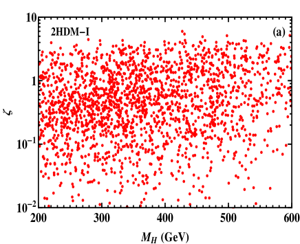
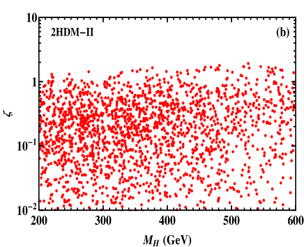
Figure 1: Parameter space in $\,M_{H}-\zeta\,$ plane for 2HDM-I [plot-(a)] and 2HDM-II [plot-(b)], where the red dots present the viable points obeying the consistency requirement of the Higgs potential as explained in the text.

Inspecting the Higgs potential (1), we derive the scalar coupling of trilinear vertex $\,Hhh$ ,

$$G_{Hhh}\, = \,\frac{\,\cos(\beta\!-\!\alpha)\,}{v}\left[\left(3M_{A}^{2}-M_{H}^{2}-2M_{h}^{2}+3\lambda_{5}v^{2}\right)\left(\cos\!2(\beta\!-\!\alpha)-\frac{\,\sin\!2(\beta\!-\!\alpha)\,}{\tan\!{2\beta}}\right)-M_{A}^{2}-\lambda_{5}v^{2}\right]$$ (14)

$$= \,\frac{\,\cos(\beta\!-\!\alpha)\,}{v}\left[\left(\frac{6M_{\!12}^{2}}{\sin\!2\beta}-M_{H}^{2}-2M_{h}^{2}\right)\left(\cos\!2(\beta\!-\!\alpha)-\frac{\,\sin\!2(\beta\!-\!\alpha)\,}{\tan\!{2\beta}}\right)-\frac{2M_{12}^{2}}{\,\sin\!2\beta\,}\right],$$

where in the second step we have used the relation $\,M_{A}^{2}+\lambda_{5}v^{2}=2M_{\!12}^{2}/\!\sin\!2\beta$ .  In the SM, the cubic Higgs coupling $\,G_{hhh}^{\text{sm}}=-3M_{h}^{2}/v\,$.  We define a coupling ratio, $\,\zeta=G_{Hhh}/G_{hhh}^{\text{sm}}\,$,  which characterizes the relative strength of the $Hhh$ coupling as compared to the $\,h^{3}\,$ Higgs coupling of the SM. Under alignment limit $\,\cos(\beta-\alpha)\rightarrow 0\,$,  the trilinear scalar coupling (14) takes the asymptotical form,

$$\zeta~{}=\,\frac{\,G_{Hhh}\,}{G_{hhh}^{\text{sm}}}~{}=~{}\frac{\,({8M_{\!12}^{2}/\!\sin\!2\beta}-\!M_{H}^{2}\!-\!2M_{h}^{2})\,}{3M_{h}^{2}}{\cos(\beta\!-\!\alpha)}+\mathcal{O}(\cos^{2}(\beta\!-\!\alpha))\,.$$ (15)

In Fig. 1, we explore the parameter space of the Higgs potential (1) in the $\,M_{H}-\zeta\,$ plane. For $\,\zeta>1\,$,  we expect that the decay branching fraction $\,\text{Br}[H\rightarrow hh]\,$ and the production cross section $\,\sigma[gg\rightarrow H\rightarrow hh]\,$ will be enhanced by the factor $\,\zeta^{2}\,$.  In Fig. 1, the red points present the viable parameter space consistent with vacuum stability, unitarity and perturbativity bounds of the Higgs potential [9]. We also take into account the $3\sigma$ constraints from the current Higgs global fit (cf. Sec. 4). The electroweak precision data also constrain the parameter space of the 2HDM. It was found that in the 2HDM the charged Higgs mass satisfies, $-600\,\textrm{GeV}<M_{H\pm}-M_{3}<100\,\textrm{GeV}$ and $M_{H\pm}>250\textrm{GeV}$ [16], where $\,M_{3}\,$ is the mass of the heaviest neutral scalar. In the case with exact $\,\mathbb{Z}_{2}$ ($M_{12}=0$), the potential could be valid up to the scale $\sim\!10\textrm{TeV}$ [17], while for the present case of a softly broken $\,\mathbb{Z}_{2}$, the bound is much more relaxed, and the theory can be valid up to the Planck scale. For the analysis of Fig. 1, we have scanned the parameter space in the following range, $\,\tan\beta\in[1,\,10]$,  $\,\cos(\beta\!-\!\alpha)\in[-0.6,\,0.6]$,  $\,M_{12}^{2}\in[-200^{2},\,200^{2}]$ GeV²,  $\,M_{H}\in[200,\,600]$ GeV, and $\,M_{A},M_{H\pm}\in[300,\,2000]$ GeV.  In the following analysis, we will consider the same range of the 2HDM parameter space unless specified otherwise.

2.2 Heavier Higgs Boson $\,\mathbf{H}^{\bf 0}$: Decays and Production

Let us consider the decay modes of the heavier neutral Higgs boson $H^{0}$.  It is straightforward to infer the tree-level decay width for $\,M_{H}>2M_{h}\,$,

$$\Gamma[H\rightarrow hh]~{}=~{}\frac{\,9\zeta^{2}M_{h}^{4}\,}{\,32\pi v^{2}M_{H}\,}\sqrt{1-\frac{4M_{h}^{2}}{M_{H}^{2}}\,}\,.$$ (16)

For $\,M_{H}\leqslant 2M_{h}\,$, we will include the off-shell decay $\,H\rightarrow hh^{*}\,$ with $\,h^{*}\rightarrow f\bar{f},\,gg,\,\gamma\gamma\,$,  etc, where $\,f\,$ denotes the light fermions except top quark. For the decay modes $\,H\rightarrow VV,\,f\bar{f}\,$,  we have $\,\Gamma[H\rightarrow VV]/\Gamma[H\rightarrow VV]_{\text{sm}}=\cos^{2}(\beta-\alpha)\,$ and $\,\Gamma[H\rightarrow f\bar{f}]/\Gamma[H\rightarrow f\bar{f}]_{\text{sm}}=(\xi_{H}^{f})^{2}\,$.  (Here, the subscript “sm” denotes the “standard model” with a reference Higgs boson $\,H\,$ which has the same mass as $\,H\,$ in the 2HDM.)  For the decay channel $\,H\rightarrow gg$ ,  we can express the partial width relative to the SM value, $\,\Gamma[H\rightarrow gg]/\Gamma[H\rightarrow gg]_{\text{sm}}=|\sum_{f=t,b}\xi_{H}^{f}A_{1/2}^{H}(\tau_{f})/A_{1/2}^{H}(\tau_{t})|^{2}\,$,  where $\,\tau_{f}=M_{H}^{2}/(4m_{f}^{2})\,$ and the function $\,A_{1/2}^{H}(\tau_{f})\,$ is the standard formula [9][18]. The decay branching ratio of $\,H\rightarrow\gamma\gamma\,$ is practically negligible for $\,M_{H}\gtrsim 200\,$GeV.  In Fig. 2, we present the decay branching fractions of the heavier Higgs boson $\,H\,$ for both 2HDM-I [plot-(a)] and 2HDM-II [plot-(b)]. For illustration, we input $\,\tan\beta=1\,$ and $\,(M_{A},\,M_{\!12}^{2})=(500\textrm{GeV},\,-(180\textrm{GeV})^{2})$  for both plots. We also set $\,\cos(\beta\!-\!\alpha)=0.4$  for plot-(a) and $\,\cos(\beta\!-\!\alpha)=0.1$  for plot-(b). We see that for $\,M_{H}<250$ GeV,  the dominant decay channels are $\,H\rightarrow ZZ,WW$,  and for $\,250\,\textrm{GeV}<M_{H}<350$ GeV,  the major decay channels include $\,H\rightarrow ZZ,WW,hh$  since the $\,H\rightarrow hh\,$ channel opens up. For $\,M_{H}>350\textrm{GeV}$, the $\,H\rightarrow t\bar{t}$  channel is further opened, and will become dominant in 2HDM-II when $\,\cos(\beta\!-\!\alpha)\,$ takes values around the alignment limit as shown in Fig. 2(b). But this situation can change when $\,\cos(\beta\!-\!\alpha)\,$ becomes larger and falls into the allowed region which separates from the alignment region (cf. Fig. 9 in Sec. 4).

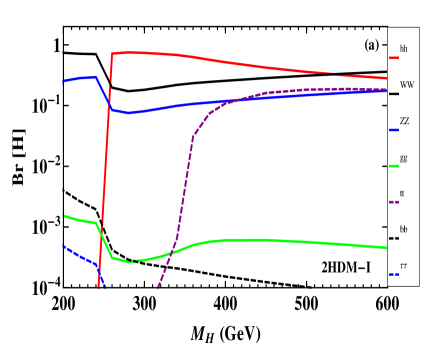
Figure 2: Decay branching fractions of the heavier Higgs state  $H^{0}$  for 2HDM-I [plot-(a)] and 2HDM-II [plot-(b)].  For illustration, we set $\,\tan\beta=1\,$ and $\,(M_{A},\,M_{\!12}^{2})=(500\textrm{GeV},\,-(180\textrm{GeV})^{2})$  for both plots. We also input $\,\cos(\beta\!-\!\alpha)=0.4$  for plot-(a) and $\,\cos(\beta\!-\!\alpha)=0.1$  for plot-(b).

From Eq. (13) and Tabel 1, we see that the Yukawa coupling of the heavier Higgs boson $H$ with $t\bar{t}$  has a scale factor $\,\xi_{H}^{t}=\sin\!\alpha/\!\sin\!\beta$  relative to the SM Higgs Yukawa coupling. The major LHC production channel is the gluon fusion process $\,gg\rightarrow H\,$.  Other production processes include the vector boson fusion $\,pp\rightarrow Hqq^{\prime}\,$,  the vector boson associated production $\,pp\rightarrow HV$,  and the top associated production $\,gg\rightarrow Ht\bar{t}\,$.  The gluon fusion production cross section of $\,H\,$ can be obtained from the corresponding SM cross section with a rescaling by $\,H\rightarrow gg\,$ partial width,

$$\sigma[gg\!\rightarrow\!H]~{}=\,\left({\Gamma[H\!\rightarrow\!gg]}/{\Gamma[H\!\rightarrow\!gg]_{\text{sm}}}\right)\sigma[gg\!\rightarrow\!H]_{\text{sm}}\,,$$ (17)

where we will include all NLO QCD corrections to the gluon fusion cross section as done in the SM case [19]. We note that for 2HDM-I, Table 1 shows that the $H$ Yukawa couplings with top and bottom quarks have the same structure as in the SM, so the $H$ production cross section $\,\sigma[gg\!\rightarrow\!H]\,$ differs from the SM by a simple rescaling factor $\,(\sin\!\alpha/\!\sin\!\beta)^{2}$.  For the 2HDM-II, we see that the $H$ coupling to $b$ quarks differs from that of $t$ quarks by a factor of $\,\tan\beta/\!\tan\!\alpha\,$,  which can enhance the $b$-loop contribution to $\,gg\!\rightarrow\!H\,$ production for large $\,\tan\beta\,$ region. Hence, the general relation (17) should be used. The uncertainty of the gluon fusion cross section is about $10\%$ over the mass-range $\,M_{H}=250-600\,$GeV [19], which is roughly the total uncertainty of signal and background calculations.

For the inclusive $\,H\,$ production, we include the gluon fusion $\,gg\rightarrow H,\,$ and $b$-related processes $b\bar{b}\rightarrow H$,  $gb\,(g\bar{b})\rightarrow Hb\,(H\bar{b})$,  and $gg\,(q\bar{q})\rightarrow Hb\bar{b}\,$.  The production cross sections for these $b$-related processes are derived by rescaling a factor of $\,(\xi_{H}^{d})^{2}$  from their corresponding SM productions with the same Higgs mass. So we have the total inclusive cross section of $\,pp\rightarrow HX\,$ for the 2HDM,

$$\sigma[pp\rightarrow HX] \!\!=\!\! \left({\Gamma[H\!\rightarrow\!gg]}/{\Gamma[H\!\rightarrow\!gg]_{\text{sm}}}\right)\sigma[pp(gg)\rightarrow H]_{\text{sm}}$$ (18)

$$+\,(\xi_{H}^{d})^{2}\left\{\sigma[pp(b\bar{b})\rightarrow H]_{\text{sm}}\!+\sigma[pp(gb,g\bar{b})\rightarrow Hb,H\bar{b}]_{\text{sm}}\!+\sigma[pp(gg,q\bar{q})\rightarrow Hb\bar{b}]_{\text{sm}}\right\}.~{}~{}~{}~{}$$

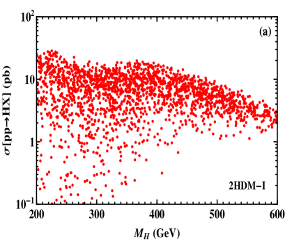
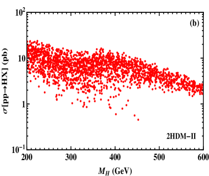
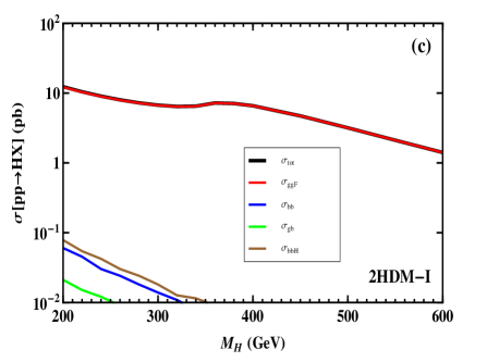
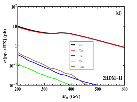
Figure 3: Inclusive $H$ production cross section via $\,pp\rightarrow HX\,$ process at the LHC (14 TeV), for 2HDM-I [plot-(a)] and 2HDM-II [plot-(b)] with $\,\tan\beta\in[1,\,10]$.  All the red points satisfy the requirements of stability, perturbativity and unitarity, as well as the $3\sigma$ constraint by the current Higgs global fit. The cross section of inclusive $H$ production $\,pp\rightarrow HX\,$ contains four sub-channels from $\,gg\rightarrow H$,  $b\bar{b}\rightarrow H$,  $gb\,(g\bar{b})\rightarrow Hb\,(H\bar{b})$,  and $\,gg\,(q\bar{q})\rightarrow Hb\bar{b}\,$.  In plot-(c) and plot-(d), we present the sub-channel contributions to the inclusive cross section $\,\sigma[pp\rightarrow HX]\,$ for 2HDM-I and 2HDM-II, respectively, where we set sample inputs, $\,\tan\beta=2\,$ and $\,\cos(\beta-\alpha)=-0.3\,(-0.1)$  for 2HDM-I (2HDM-II). In plots (c)-(d), the red curve ($gg\rightarrow HX$ contribution) and the black curve (summed total contribution) fully overlap because the $\,gg\rightarrow HX\,$ channel dominates the inclusive cross section in the low $\tan\beta$ region.

We present the inclusive $\,H\,$ production rate for 2HDM Type-I and Type-II in Fig. 3(a)-(b). Multiplying the production cross section with decay branching fraction $\text{Br}(H\!\rightarrow\!hh\!\rightarrow\!WW^{*}\gamma\gamma)$,  we compute the signal rate in the channel $\,pp\!\rightarrow\!HX\,$ with $\,H\!\rightarrow\!hh\!\rightarrow\!WW^{*}\gamma\gamma$ .  We summarize our results in Fig. 4 for 2HDM-I and 2HDM-II, respectively. In Fig. 3(a)-(b) and Fig. 4(a)-(b), we have scanned the same 2HDM parameter space as in Fig. 1. The signal process is depicted by the left diagram of Fig. 5. From Fig. 4, we see that the cross section $\,\sigma(pp\!\rightarrow\!HX)\times\text{Br}(H\!\rightarrow\!hh\!\rightarrow\!WW^{*}\gamma\gamma)$  can be as large as about $70$ fb for 2HDM-I; while for 2HDM-II, this cross section can reach about $10$ fb for $\,M_{H}\lesssim 340$ GeV .

For comparison, we show the individual contributions of each sub-channel to the total inclusive cross section $\,\sigma[pp\rightarrow HX]\,$ in Fig. 3(c)-(d). For illustrations, we set sample parameter inputs, $\,\tan\beta=2\,$ and $\,\cos(\beta-\alpha)=-0.3$  for 2HDM-I, and $\,\tan\beta=2\,$ and $\,\cos(\beta-\alpha)=-0.1\,$ for 2HDM-II. In plots (c)-(d), the red curve ($gg\rightarrow H$ contribution) fully overlaps the black curve (summed total contribution). This is because the gluon fusion channel $\,gg\rightarrow H\,$ dominates the inclusive production cross section for low $\,\tan\beta\,$ region of the 2HDM. In general, Table 1 shows that for 2HDM-I, the $H$ Yukawa couplings ($\,\xi^{u}_{H}=\xi^{d}_{H}=\sin\alpha/\!\sin\beta\,$) are rather insensitive to $\tan\beta$ .  Hence, in 2HDM-I the gluon fusion actually dominates the $\,H$  production over full range of $\,\tan\beta\geqslant 1$,  and the contributions of $b$-related sub-channels are always negligible. For 2HDM-II, the (up-type) $H$ Yukawa coupling $\,\xi^{u}_{H}=\sin\alpha/\!\sin\beta\,$ is the same as 2HDM-I, and the down-type Yukawa coupling $\,\xi^{d}_{H}\propto 1/\!\cos\beta=\tan\beta/\!\sin\beta\,$ is enhanced by a $\,\tan\beta\,$ factor relative to $\,\xi^{u}_{H}\,$.  We find that for small $\,\tan\beta\lesssim 3\,$,  the gluon fusion channel still dominates the inclusive $\,H$  production in 2HDM-II, and its cross section is larger than other $b$-related channels by a factor of $\,O(10\!-\!100)\,$ for $M_{H}\geqslant 300$ GeV.  The analysis of 2HDM-II in Sec. 4 also concerns the small $\,\tan\beta\,$ region [cf. Fig. 9(b)(d)]. Hence, in the following Sec. 3–4, we will focus our analysis on the Higgs production from gluon fusion channel, $pp(gg)\rightarrow H\rightarrow hh\rightarrow WW^{*}\gamma\gamma$ .

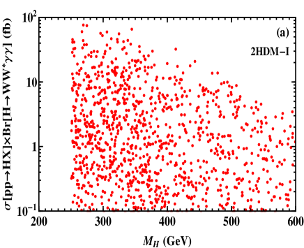
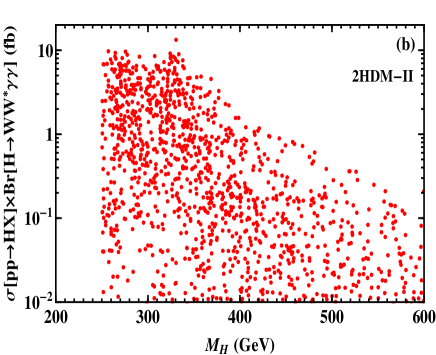
Figure 4: LHC signal cross section $\,\sigma(pp\!\rightarrow\!HX)\!\times\!\text{Br}(H\!\rightarrow\!hh\!\rightarrow\!WW^{*}\gamma\gamma)$  in the 2HDM with $\,\tan\beta\in[1,\,10]$.  Plots (a) and (b) present the results for 2HDM-I and 2HDM-II, respectively.

3 Higgs Signal and Background Simulations

In this section, we compute the Higgs signals and backgrounds at the LHC (14 TeV). We perform systematical simulations by using MadGraph5 package [21] for the process, $\,pp(gg)\!\rightarrow\!H\!\rightarrow\!hh\!\rightarrow\!WW^{*}\gamma\gamma$,  via gluon fusion channel. The parton-level Higgs production cross section $\sigma(gg\rightarrow H)$ is derived from Eq. (17), including NLO QCD corrections. We illustrate the signal Feynman diagram by the left plot of Fig. 5. For signal process, we generate the model file using FeynRules [22], containing $\,Hhh\,$ vertex and the effective $\,ggH\,$ vertex. We compute signal and background events using MadGraph5/MadEvent [21]. Then, we apply Pythia [23] to simulate hadronization of partons and adopt Delphes [24] to perform detector simulations.

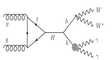
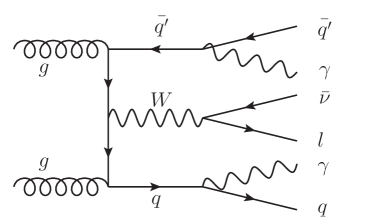
Figure 5: LHC production process $\,gg\rightarrow WW\gamma\gamma$ .  The left diagram shows the signal production via $\,gg\rightarrow H\rightarrow hh\rightarrow WW\gamma\gamma\,$,  and the right diagram illustrates an irreducible background process $\,gg\rightarrow q\bar{q^{\prime}}\ell\bar{\nu}\gamma\gamma\,$.

For the final state $WW$ decays, we will study both the pure leptonic mode $\,WW\rightarrow\ell\nu\ell\nu\,$ and the semi-leptonic mode $\,WW\rightarrow q\bar{q}^{\prime}\ell\nu$.  The $W$ decay branching fractions to $\,e\nu\,$ and $\,\mu\nu\,$ equal 10.8% and 10.6%, respectively, while that of $\,W\rightarrow\tau\nu\,$ is about 11.3% [25]. The dijet branching ratio of $\,W\rightarrow q\bar{q}^{\prime}\,$ equals 67.6% [25]. Thus, the inclusion of semi-leptonic mode will be beneficial. Since $\,\tau\,$ leptons can decay into $\,e,\mu$ ,  the detected final state $\,e,\mu$  will include those from the $\tau$ decays. For $\,M_{h}=125\,$GeV,  the branching fraction of $\,h\rightarrow\gamma\gamma\,$ in the SM equals $\,2.3\times 10^{-3}\,$ [18]. In the following, we will first present the analyses for $\,M_{H}=300\,$GeV in Sec. 3.1–3.2, and then for heavier masses $\,M_{H}=400,600\,$GeV in Sec. 3.3.

3.1 Pure Leptonic Channel: ${hh\rightarrow\!WW^{*}\gamma\gamma\!\rightarrow\ell\nu\ell\nu\gamma\gamma}$

For pure leptonic channel, we have $\,hh\rightarrow WW^{*}\gamma\gamma\rightarrow\ell\nu\ell\nu\gamma\gamma\,$.  Although this channel has an event rate about two orders of magnitude lower than that of $\,hh\rightarrow b\bar{b}\gamma\gamma$  mode, it has much cleaner background as compared to $\,b\bar{b}\gamma\gamma$  final state. After imposing simple cuts, we find that the backgrounds can be substantially reduced. We follow the ATLAS procedure for event selections. To discriminate the Higgs signal from backgrounds, we set up preliminary event selection by requiring two leptons (electron or muon) and at least two photons in the final state,

$$n_{\ell}=2\,,\qquad n_{\gamma}\geqslant 2\,.$$ (19)

In the first step of event analysis, we need to prevent the potential double-counting, i.e., the reconstructed objects are required to have a minimal spatial separation [26]. The two leading photons are always kept, but we impose the following criteria [26]: (i) electrons overlapping with one of those photons within a cone $\,\Delta R(e,\gamma)<0.4$  are rejected; (ii) jets within $\,\Delta R(\text{jet},e)<0.2$  or $\,\Delta R(\textrm{jet},\gamma)<0.4$  are rejected; (iii) muons within a cone of $\,\Delta R(\mu,\textrm{jet})<0.4$  or $\Delta R(\mu,\gamma)<0.4$  are rejected. After this, we apply the basic cuts to take into account the detector conditions, which are imposed as follows,

$$P_{T}(\gamma),P_{T}(q)>25\,\mathrm{GeV},\quad P_{T}(\ell)>15\,\mathrm{GeV},\quad|\eta(\gamma)|,|\eta(q)|,|\eta(\ell)|<2.5\,.$$ (20)

Table 2: Signal and background cross sections of $\,pp\rightarrow WW^{*}\gamma\gamma\rightarrow\ell\nu\ell\nu\gamma\gamma$  and $\,pp\rightarrow WW^{*}\gamma\gamma\rightarrow q\bar{q}^{\prime}\ell\nu\gamma\gamma$  processes at the LHC (14 TeV) after each set of cuts. The signal significance($Z_{0}$) is computed for the LHC (14 TeV) runs with 300 fb^-1 integrated luminosity. We input the heavier Higgs mass $\,M_{H}=300\,$GeV,  and set the sample signal cross section as $\,\sigma(pp\!\rightarrow\!H\!\rightarrow\!hh\!\rightarrow\!WW^{*}\gamma\gamma)=5\,\mathrm{fb}$ . From the 3rd to 5th columns, we show the signals and backgrounds after imposing each set of cuts. The “Selection + Basic Cuts” are choosing according to Eqs. (19)–(20). In the pure leptonic mode, we impose the Final Cuts $M_{T}(\ell\ell\nu\nu),M(\ell\ell)$,  $M_{T}(\ell\ell\nu\nu\gamma\gamma)$,  $\Delta\phi(\ell\ell)$,  $\Delta R(\ell\ell)$,  and $\Delta R(\gamma\gamma)$.  In the semi-leptonic mode, we add the Final Cuts $P_{T}(\gamma)$  $\,M_{T}(q\bar{q}^{\prime}\!\ell\nu)$,  and $\Delta R(\gamma\gamma)$. 

$\,pp\rightarrow\ell\nu\ell\nu\gamma\gamma$	Sum	Selection+Basic Cuts	$M_{\gamma\gamma},E\!\!\!/_{T}$	Final Cuts
Signal (fb)	0.525	0.0251	0.0214	0.0161
BG$[\ell\nu\ell\nu\gamma\gamma\!+\!\ell\ell\gamma\gamma]$ (fb)	153.3	0.937	0.00225	0.000215
BG$[t\bar{t}h]$ (fb)	0.0071	0.000493	0.000419	0.000076
BG$[Zh]$ (fb)	0.175	0.0331	0.00210	0.000078
BG$[hh]$ (fb)	0.00222	0.000132	0.000102	0.000062
BG[Total] (fb)	153.48	0.971	0.00488	0.00043
Significance($Z_{0}$)	0.734	0.439	3.70	5.15
$\,pp\rightarrow q\bar{q}^{\prime}\ell\nu\gamma\gamma$	Sum	Selection+Basic Cuts	$M_{\gamma\gamma}$, $M_{qq}$, $E\!\!\!/_{T}$	Final Cuts
Signal (fb)	2.2	0.124	0.0937	0.0749
BG$[q\bar{q}^{\prime}\!\ell\nu\gamma\gamma]$ (fb)	31.59	0.580	0.0192	0.00912
BG$[\ell\nu\gamma\gamma]$ (fb)	143.3	0.0642	0.00349	0.00182
BG$[Wh]$ (fb)	0.42	0.00509	0.00234	0.00140
BG$[WWh]$ (fb)	0.0023	0.000210	0.000104	0.000050
BG[$t\bar{t}h$] (fb)	0.0148	0.00163	0.000802	0.000420
BG[$hh$] (fb)	0.00462	0.000291	0.000160	0.000106
BG[$th$] (fb)	0.0129	0.000479	0.000186	0.000099
BG[Total] (fb)	175.35	0.652	0.0264	0.0130
Significance($Z_{0})$	2.87	2.59	7.29	7.47

Next, we turn to the background analysis for pure leptonic mode. Besides the $\,\ell\nu\ell\nu\gamma\gamma\,$ and $\,\ell\ell\gamma\gamma\,$ backgrounds, there are additional reducible backgrounds from Higgs bremstrahlung, vector boson fusion, and $t\bar{t}h$ production. The cross section of the former two processes are fairly small and thus negligible for the present study. The $t\bar{t}h$ associate production, with $\,t\bar{t}\rightarrow WWb\bar{b}\,$, can be important because the diphoton invariant-mass cut does not effectively discriminate the signal process. But, this background can be suppressed by imposing $b$-veto [27]. The production cross section for $\,t\bar{t}h\,$ in the SM is $\,\sigma(pp\rightarrow t\bar{t}h)=0.6113$ pb [28]. The latest $b$-veto efficiency of ATLAS is, $\,\epsilon(b\mathrm{-veto})=22\%$  [29]. Thus, we estimate the cross section for this background process,

$$\sigma(pp\!\rightarrow\!t\bar{t}h\!\rightarrow\!\ell\nu\ell\nu\gamma\gamma)\,=\,\sigma(pp\!\rightarrow\!t\bar{t}h)\times\mathrm{Br}[W\!\rightarrow\!\ell\nu]^{2}\,\mathrm{Br}[h\!\rightarrow\!\gamma\gamma]\,\epsilon(b\mathrm{-veto})^{2}\simeq 7.28\!\times\!10^{-3}\,\mathrm{fb}\,,~{}~{}~{}~{}~{}$$ (21)

where $\,W\!\rightarrow\!\ell\nu\,$ includes $\,\ell=e,\mu,\tau$.  We see that imposing the $b$-veto has largely suppressed the $\,t\bar{t}h$  background. We note that the $\,t\bar{t}h\,$ background is much smaller than the $\,\ell\nu\ell\nu\gamma\gamma\,$ background before kinematic cuts, while after all the kinematic cuts it could be non-negligible. So we will include both for the present background analysis.

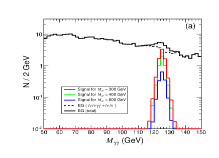
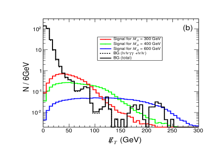
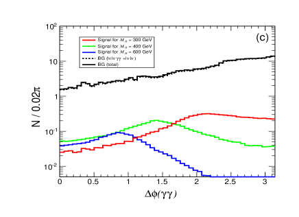
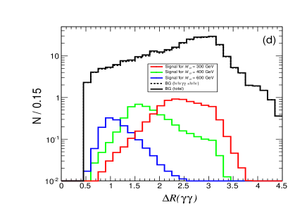
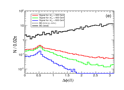
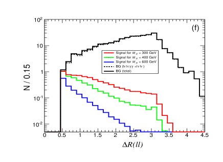
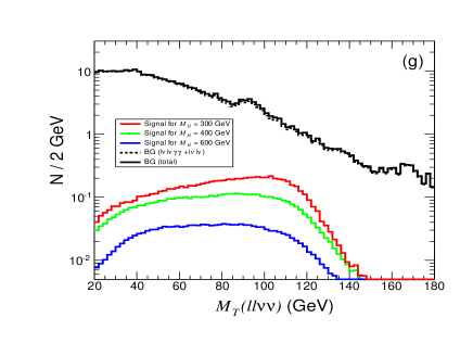
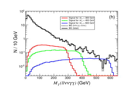
Figure 6: Signal and background distributions in the pure leptonic channel $\,hh\rightarrow WW^{*}\rightarrow\ell\nu\ell\nu\,$ before imposing kinematical cuts. For comparison, we plot the signal distributions for $\,M_{H}=(300,\,400,\,600)\,$GeV by (red, green, blue) curves. We present plot-(a) for $\,M_{\gamma\gamma}\,$ distribution, plot-(b) for $E\!\!\!/_{T}$ distribution, plot-(c) for $\,\Delta\phi(\gamma\gamma)\,$ distribution, plot-(d) for $\,\Delta R(\gamma\gamma)\,$ distribution, plot-(e) for $\,\Delta\phi(\ell\ell)\,$ distribution, plot-(f) for $\,\Delta R(\ell\ell)\,$ distribution, plot-(g) for $\,M_{T}(\ell\ell\nu\nu)\,$ distribution, and plot-(h) for $\,M_{T}(\ell\ell\nu\nu\gamma\gamma)\,$ distribution, respectively.

Another potential background may arise from the Higgs pair production $\,pp\rightarrow hh\,$ in the SM [30, 31, 32]. Our signal process $\,pp\rightarrow H\,$ produces on-shell Higgs boson $H$ with decays $\,H\rightarrow hh\,$,  which has much larger rate as well as rather different kinematics from the non-resonant di-Higgs production in the SM. (Since our signal has on-shell $H$ production, we find that its interference with the SM-type non-resonant $hh$ production is negligible after kinematical cuts.) For instance, we can further suppress this SM di-Higgs contribution by imposing a cut on the transverse mass of di-Higgs bosons.

We also consider a reducible background from the $Zh$ associate production. The SM cross section of this process $\,pp\rightarrow Zh\,$ at the LHC is $\,\sigma(pp\rightarrow Zh)=0.761$ pb [18]. Hence, this background gives $\,\sigma(pp\rightarrow Zh\rightarrow\ell\ell\gamma\gamma)=0.175$ fb before any cuts. Because the $Zh$ background must have the invariant mass $\,M(\ell\ell)\,$ of final state di-leptons peaked at $\,M_{Z}\simeq 91.2$ GeV,  we can efficiently kill this background by applying a narrow cut on $\,M(\ell\ell)\,$,  which has little effect on the signal rate. In the present analysis, we choose, $\,M(\ell\ell)\in(M_{Z}\!-\!5\Gamma_{Z},\,M_{Z}\!+\!5\Gamma_{Z})$,  where $\Gamma_{Z}\simeq 2.5\,\textrm{GeV}$ is the total width of $Z$ boson. Other reducible backgrounds come from the fake events in which quark and/or gluon are misidentified as photons. These backgrounds include $\,\ell\nu\ell\nu q\gamma$,  $\ell\nu\ell\nu g\gamma$,  $\ell\nu\ell\nu qq$,  $\ell\nu\ell\nu qg$,  and $\,\ell\nu\ell\nu gg$ .  For our analysis, we adopt the fake rates used by ATLAS detector [33],

$$\epsilon_{q\rightarrow\gamma}\simeq 3.6\times 10^{-4},\qquad\epsilon_{g\rightarrow\gamma}\simeq 3.6\times 10^{-5}.$$ (22)

With such small fake rates, we find that these reducible backgrounds are negligible.

In summary, with the above considerations of the SM backgrounds, we will compute the irreducible backgrounds with final state $\,\ell\nu\ell\nu\gamma\gamma$ ,  and the reducible backgrounds including the $\,\ell\ell\gamma\gamma$  final state, the $\,t\bar{t}h$  associate production, the $Zh$ associate production, and the SM di-Higgs production.

In Fig. 6, we present the distributions of relevant kinematical variables for the pure leptonic channel, including both signals and backgrounds. In this figure, we show the signal distributions at the LHC (14TeV) with 300 fb^-1 integrated luminosity for $\,M_{H}=(300,\,400,\,600)\,$GeV by (red, green, blue) curves as well as the backgrounds (black curves). Here we have input the sample cross section $\,\sigma(pp\!\rightarrow\!H\!\rightarrow\!hh\!\rightarrow\!WW^{*}\gamma\gamma)=(5,\,3,\,1)$ fb for $\,M_{H}=(300,\,400,\,600)\,$GeV, respectively. In the following, we will analyze how to effectively suppress the SM backgrounds by implementing proper kinematical cuts.

From Fig. 6(a)-(b), we first impose kinematical cuts on the diphotons invariant-mass $\,M_{\gamma\gamma}\,$ and the missing energy $E\!\!\!/_{T}$ of final state neutrinos,

$$120\,\mathrm{GeV}<M_{\gamma\gamma}<130\,\mathrm{GeV},\hskip 22.76219ptE\!\!\!/_{T}>20\,\mathrm{GeV}\,.$$ (23)

The missing energy cut can also sufficiently remove the $\,\ell\ell\gamma\gamma\,$ background.

Then, inspecting Fig. 6(c)-(f), we apply the kinematical cuts on the azimuthal angle $\,\Delta\phi\,$ and opening angle $\,\Delta R\,$ for the final state di-leptons and di-photons, respectively,

$$\Delta\phi(\ell\ell)<2.0\,,\qquad\Delta R(\ell\ell)<3.0\,,\qquad\Delta R(\gamma\gamma)<3.8\,.$$ (24)

Here, from the distributions of Fig. 6(c), we find that the $\,\Delta\phi(\gamma\gamma)\,$ cut is not effective for Higgs mass $\,M_{H}=300\,$GeV. So we do not implement this cut.

For the transverse mass cut [25], we consider the transverse mass $\,M_{T}\,$ for the $\ell\ell\nu\nu$ system with two leptons and missing energy, which should be no larger than the Higgs mass $\,M_{h}\simeq 125$ GeV.  All the final state leptons/neutrinos are nearly massless, so the transverse energy of each final state equals its transverse momentum $\,E_{T,i}\simeq|\vec{P}_{T,i}|$ ,  ($i=1,2,3$),  where $\,i=1,2\,$ denote two leptons $\,\ell_{1,2}\,$ and $\,i=3\,$ denotes the system of two neutrinos. Thus, we have

$$M_{T}^{2}\,=\,\left(E_{T,1}+E_{T,2}+E_{T,3}\right)^{2}-(\vec{P}_{T,1}+\vec{P}_{T,2}+\vec{P}_{T,3})^{2}\,\simeq\sum_{1\leqslant i<j\leqslant 3}\!\!2E_{T,i}E_{T,j}(1\!-\cos\phi_{ij})\,.$$ (25)

With this and inspecting Fig. 6(g), we implement the transverse mass cut,

$$M_{T}(\ell\ell\nu\nu)<135\,\textrm{GeV}.$$ (26)

From Fig. 6(h), we will further impose the transverse mass cut for the full final state $\,\ell\ell\nu\nu\gamma\gamma$ ,

$$60\textrm{GeV}\,<\,M_{T}(\ell\ell\nu\nu\gamma\gamma)\,<\,320\,\mathrm{GeV}\,.$$ (27)

The kinematical cuts for the cases of $\,M_{H}=400$ GeV and $\,600\,$GeV will be discussed in Sec. 3.3.

We summarize the results in Table 2 for both signal and backgrounds. For demonstration, we first input the heavier Higgs mass $\,M_{H}=300\,$GeV,  and set the sample signal cross section $\,\sigma(pp\!\rightarrow\!H\!\rightarrow\!hh\!\rightarrow\!WW^{*}\gamma\gamma)=5\,\mathrm{fb}$  for the LHC (14 TeV). In Table 2, we also show the significance of signal over backgrounds after each set of kinematical cuts at the LHC Run-2 with 300 fb^-1 integrated luminosity. When the event number is small, we can use the median significance($Z_{0}$) (instead of $\,S/\!\sqrt{B}$ ), as defined in following [34],

$$Z_{0}=\sqrt{2\left[(S\!+\!B)\ln\left(\frac{\,S\!+\!B\,}{B}\right)-S\!\right]\,}\,.$$ (28)

As shown in Table 2, after applying all kinematical cuts, we estimate the signal significance$(Z_{0})=5.15$ .

3.2 Semi-leptonic Channel: $hh\rightarrow\!WW^{*}\gamma\gamma\!\rightarrow q\bar{q}^{\prime}\ell\nu\,\gamma\gamma$

The analysis of semi-leptonic channel $\,WW^{*}\!\rightarrow q\bar{q}^{\prime}\ell\nu\,$ is similar to that of the pure leptonic mode $\,WW^{*}\!\rightarrow\ell\nu\ell\nu\,$.  But, there are nontrivial differences. One thing is that for each decay we need to specify which decay mode is from on-shell $W$ ($q\bar{q}^{\prime}$ or $\ell\nu$), since these two situations have different distributions. To illustrate this, we present the distribution of $M_{qq}$ in Fig. 7(a), where the green (blue) curve depicts the final state $qq$ from on-shell (off-shell) $W$ decays, and the red curve represents the actual distribution of $M_{qq}$ from $\,WW^{*}\!\rightarrow q\bar{q}^{\prime}\ell\nu\,$.  Fig. 7(a) shows that the $M_{qq}$ distribution from on-shell $W$ decays (green curve) has event rate peaked around $\,M_{qq}\!=70-80$ GeV ,  while the $M_{qq}$ distribution from off-shell $W$ decays (blue curve) is rather flat.

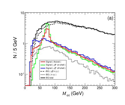
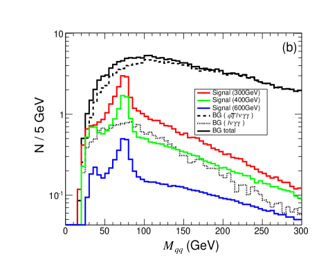
Figure 7: Invariant-mass distribution of $\,M_{qq}$  for semi-leptonic decay channel $\,WW^{*}\rightarrow q\bar{q}^{\prime}\!\ell\nu\,$ at the LHC (14TeV) with 300 fb^-1 integrated luminosity. Plot-(a) shows the mode with on-shell (off-shell) decays $\,W\,(W^{*})\rightarrow q\bar{q}^{\prime}\,$ by green (blue) curve, for $\,M_{H}=300$ GeV.  The red curve corresponds to the realistic decays of $\,WW^{*}\rightarrow q\bar{q}^{\prime}\!\ell\nu\,$.  Plot-(b) presents the $\,M_{qq}$  distribution for full signals of $\,WW^{*}\rightarrow q\bar{q}^{\prime}\!\ell\nu\,$ by (red, green, blue) curves for $\,M_{H}=(300,\,400,\,600)$ GeV. In each plot, the black solid curve gives the full backgrounds.

Our first step here is also to remove the pileup events, similar to Sec. 3.1. Then, we select the final states by imposing the preliminary cuts

$$n_{j}\geqslant 2\,,\quad n_{\gamma}\geqslant 2\,,\quad n_{\ell}=1\,.$$ (29)

For jets we choose the leading and subleading pair, while for photons we choose the diphoton pair whose $\,M_{\gamma\gamma}\,$ is closet to $\,M_{h}=125\,$GeV.  Then, we choose the basic cuts to be the same as in Eq. (20).

Next, we turn to the background analysis. The most important background for this channel comes from the SM irreducible background, $\,pp\!\rightarrow\!q\bar{q}^{\prime}\ell\nu\gamma\gamma\,$,  whose cross section is about  $\sigma[q\bar{q}^{\prime}\ell\nu\gamma\gamma]\simeq 31.6$ fb.  Another significant reducible background is the SM process $\,pp\rightarrow\ell\nu\gamma\gamma\,$,  which has a cross section  $\sigma[\ell\nu\gamma\gamma]\simeq 143$ fb .  But this will be mainly rejected by the jet-selections in Eq. (29). For the $\,t\bar{t}h\,$ background, we find that under $b$-veto its cross section is $\,0.0148$ fb, as shown in Table 2. Single top associated Higgs production gives another background, $\,\sigma[pp\rightarrow th(\bar{t}h)+X]=79.4$ fb [35], where $\,X\,$ represents single-jet or dijets in our simulation. We find that under $b$-veto this cross section of $\,pp\rightarrow th(\bar{t}h)+X\rightarrow b\ell\nu\gamma\gamma+X\,$ reduces to about $\,0.013$ fb .  We also include the non-resonant di-Higgs production in the SM, which has much smaller event rate and rather different kinematics. Other potential SM backgrounds may include the reducible backgrounds such as $\,qq\ell\nu gg\,$ with $\,gg\,$ misidentified as $\,\gamma\gamma\,$. This is actually negligible due to the tiny $\,g\rightarrow\gamma\,$ misidentification rate shown in Eq. (22).

For the kinematic cuts, we choose the $\,M_{\gamma\gamma}$ cut as in Eq. (23). The invariant-mass $\,M_{qq}$ should match the $W$ mass. We depict the $\,M_{qq}$ distribution in Fig. 7. Plot-(a) depicts the decay mode with on-shell (off-shell) decays $\,W\,(W^{*})\rightarrow q\bar{q}^{\prime}\,$ by green (blue) curve, for $\,M_{H}=300$ GeV.  The realistic decays of $\,WW^{*}\rightarrow q\bar{q}^{\prime}\!\ell\nu\,$ correspond to the red curve. In plot-(b), we present the $\,M_{qq}$  distribution for full signals of $\,WW^{*}\rightarrow q\bar{q}^{\prime}\!\ell\nu\,$ by (red, green, blue) curves for $\,M_{H}=(300,\,400,\,600)$ GeV. The black solid curve in each plot gives the full backgrounds. From Fig. 7, we choose the $\,M_{qq}$ cut,

$$M_{qq}<\,250\,\mathrm{GeV}.$$ (30)

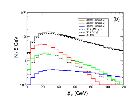
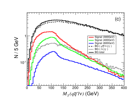
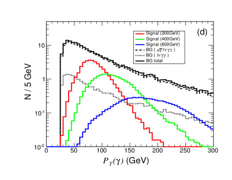
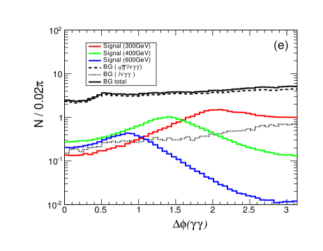
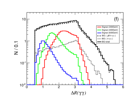
Figure 8: Signal and background distributions for semi-leptonic channel $\,hh\rightarrow WW^{*}\rightarrow q\bar{q}^{\prime}\!\ell\nu\gamma\gamma$  before imposing kinematical cuts. For comparison, we plot the signal distributions for $\,M_{H}=(300,\,400,\,600)\,$GeV by (red, green, blue) curves. We present the $\,M_{\gamma\gamma}$ distribution in plot-(a), the missing $E\!\!\!/_{T}$ distribution in plot-(b), the $\,M_{T}(q\bar{q}^{\prime}\!\ell\nu)\,$ distribution in plot-(c), the $P_{T}(\gamma)$ distribution of the leading photon in plot-(d), the $\,\Delta\phi(\gamma\gamma)\,$ distribution in plot-(e), and the $\,\Delta R(\gamma\gamma)\,$ distribution in plot-(f), respectively.

We present the distributions for other kinematical observables in Fig. 8, where we have input the sample cross section $\,\sigma(pp\!\rightarrow\!H\!\rightarrow\!hh\!\rightarrow\!WW^{*}\gamma\gamma)=(5,\,3,\,1)$ fb  for $\,M_{H}=(300,\,400,\,600)\,$GeV.  From Fig. 8(a)-(b), we impose cuts on the diphoton invariant-mass $\,M_{\gamma\gamma}\,$ and the missing energy $\,E\!\!\!/_{T}$ of final state neutrinos,

$$120\,\mathrm{GeV}<M_{\gamma\gamma}<130\,\mathrm{GeV},\hskip 22.76219pt10\,\textrm{GeV}<E\!\!\!/_{T}<80\,\mathrm{GeV}.$$ (31)

We require $\,E\!\!\!/_{T}>10\,$GeV to suppress certain reducible backgrounds, as also adopted in the ATLAS analysis. For instance, consider the background $\,qq\gamma\gamma\!+\!j$  with $j$ mistagged as a lepton, where $j$ denotes a gluon or quark jet. Since it contains no neutrino in the final state, we can eliminate it by imposing the missing energy $\,E\!\!\!/_{T}$ cut. This is more like a basic cut. For the transverse momentum distribution of the leading photon shown in Fig. 8(d), we set the following cut,

$$60\,\mathrm{GeV}<\,P_{T}(\gamma)\,<150\,\mathrm{GeV}.$$ (32)

Then, we inspect the transverse mass distribution of $\,q\bar{q}^{\prime}\ell\nu$  final state, which arises from the decay products of $\,h\!\rightarrow\!WW^{*}\!\!\rightarrow\!q\bar{q}^{\prime}\ell\nu\,$.  From Fig. 8(c), we impose the following cut,

$$M_{T}(q\bar{q}^{\prime}\!\ell\nu)\,<\,200\,\mathrm{GeV}.$$ (33)

With Fig. 8(e)-(f), we have also examined possible cuts on $\,\Delta\phi(\gamma\gamma)\,$ and $\,\Delta R(\gamma\gamma)\,$ distributions. We further impose,

$$1\,<\,\Delta R(\gamma\gamma)\,<\,3.8\,.$$ (34)

We summarize our results in Table 2. Here we present the signal and background cross sections after each set of cuts. We take an integrated luminosity of $300\,\mathrm{fb}^{-1}$ for the LHC (14 TeV), and derive the corresponding signal significance($Z_{0}$). Under all cuts, we estimate the final significance of the signal detection to be $\,7.47\,$ in the semi-leptonic channel $\,q\bar{q}^{\prime}\ell\nu\gamma\gamma$ ,  as shown in Table 2.

Table 3: Signal and background cross sections of both $\,pp\rightarrow WW^{*}\gamma\gamma\rightarrow\ell\nu\ell\nu\gamma\gamma$  and $\,pp\rightarrow WW^{*}\gamma\gamma\rightarrow q\bar{q}^{\prime}\ell\nu\gamma\gamma$ processes at the LHC (14 TeV) after each set of cuts. The signal significance($Z_{0}$) is computed for the LHC (14 TeV) runs with 300 fb^-1 integrated luminosity. We input the heavier Higgs mass $\,M_{H}=400\,$GeV,  and set the sample signal cross section $\,\sigma(pp\!\rightarrow\!H\!\rightarrow\!hh\!\rightarrow\!WW^{*}\gamma\gamma)=3\,\mathrm{fb}$ .  From the 3rd to 5th columns, we present the signals and backgrounds after imposing each set of cuts. In the pure leptonic mode, we impose the Final Cuts $M_{T}(\ell\ell\nu\nu)$,  $M(\ell\ell)$,  $M_{T}(\ell\ell\nu\nu\gamma\gamma)$,  $\Delta\phi(\ell\ell)$,  $\Delta R(\ell\ell)$,  $\Delta\phi(\gamma\gamma)$,  and $\Delta R(\gamma\gamma)$.  In the semi-leptonic mode, we add the Final Cuts $P_{T}(\gamma)$,  $M_{T}(q\bar{q}^{\prime}\!\ell\nu)$,  $\Delta\phi(\gamma\gamma)$,  and $\Delta R(\gamma\gamma)$.

$\,pp\rightarrow\ell\nu\ell\nu\gamma\gamma$	Sum	Selection+Basic Cuts	$M_{\gamma\gamma},E\!\!\!/_{T}$	Final Cuts
Signal (fb)	0.315	0.0165	0.0147	0.0107
BG[$\ell\nu\ell\nu\gamma\gamma\!+\!\ell\ell\gamma\gamma$] (fb)	153.3	0.937	0.00394	0.000169
BG$[t\bar{t}h]$ (fb)	0.0071	0.000493	0.000452	0.000051
BG$[Zh]$ (fb)	0.175	0.0331	0.00247	0.000065
BG$[hh]$ (fb)	0.00222	0.000132	0.000116	0.000074
BG[Total] (fb)	153.48	0.971	0.00698	0.000359
Significance($Z_{0}$)	0.440	0.289	2.44	4.05
$\,pp\rightarrow q\bar{q}^{\prime}\!\ell\nu\gamma\gamma$	$\sigma_{\mathrm{t}otal}$	Selection+Basic Cuts	$M_{\gamma\gamma}$, $M_{qq}$, $E\!\!\!/_{T}$	Final Cuts
Signal (fb)	1.32	0.0891	0.0671	0.0533
BG[$qq\ell\nu\gamma\gamma$] (fb)	31.59	0.581	0.0291	0.00672
BG[$\ell\nu\gamma\gamma$] (fb)	143.3	0.0642	0.00454	0.000891
BG[$Wh$] (fb)	0.42	0.00509	0.00335	0.00139
BG[$WWh$] (fb)	0.0023	0.000210	0.000127	0.000057
BG[$t\bar{t}h$] (fb)	0.0148	0.00163	0.00111	0.000441
BG[$hh$] (fb)	0.00462	0.000291	0.000197	0.000155
BG[$th$] (fb)	0.0129	0.000479	0.000247	0.000104
BG[Total] (fb)	175.35	0.653	0.0386	0.0098
Significance($Z_{0}$)	1.72	1.87	4.86	6.22

3.3 Analyses of Heavier Higgs Boson with 400 GeV and 600 GeV Masses

For signal and background analyses in Sec. 3.1–3.2, we have set the mass of heavier Higgs boson $\,M_{H}=300\,$GeV for demonstration. In this subsection, we turn to the analyses for other sample inputs of Higgs mass, $\,M_{H}=400\,\textrm{GeV}$  and $\,M_{H}=600\,\textrm{GeV}$.  We demonstrate how the analysis and results may vary as the Higgs mass increases. These are parallel to what we have done in Sec. 3.1–3.2.

For the heavier Higgs boson with mass $\,M_{H}=400$ GeV,  from the distributions in Fig. 6, we choose the following kinematical cuts for the pure leptonic channel,

$$120\,\mathrm{GeV}<M_{\gamma\gamma}<130\,\mathrm{GeV},\hskip 14.22636pt\Delta\phi(\gamma\gamma)<2.5\,,\hskip 14.22636pt\Delta R(\gamma\gamma)<2.5\,,$$

$$E\!\!\!/_{T}>20\,\mathrm{GeV},\hskip 14.22636ptM_{T}(\ell\ell\nu\nu)<135\,\textrm{GeV},\hskip 14.22636pt75\textrm{GeV}<M_{T}(\ell\nu\ell\nu\gamma\gamma)<420\,\mathrm{GeV},\hskip 19.91692pt$$ (35)

$$\Delta\phi(\ell\ell)<2.0\,,\hskip 14.22636pt\Delta R(\ell\ell)<2.2\,,\hskip 14.22636ptM(\ell\ell)~{}\setminus\in(M_{Z}\!-\!5\Gamma_{Z},M_{Z}\!+\!5\Gamma_{Z})\,.$$

Comparing with the previous case of $\,M_{H}=300$ GeV,  we find that the distributions $\,\Delta\phi(\ell\ell)$,  $\,\Delta R(\ell\ell)$,  $\,\Delta\phi(\gamma\gamma)$,  and $\,\Delta R(\gamma\gamma)\,$ damp faster in the larger $\,\Delta\phi\,$ and $\,\Delta R$  regions, as shown in Fig. 6. This is because the di-Higgs bosons are more boosted in the $\,H\rightarrow hh\,$ decays with heavier mass $\,M_{H}=400$ GeV .  We present the cut efficiency for the case of $\,M_{H}=400\,$GeV  in Table 3, where we set a sample signal cross section $\,\sigma(pp\!\rightarrow\!H\!\rightarrow\!hh\!\rightarrow\!WW^{*}\gamma\gamma)=3\,\mathrm{fb}$ .  In this case, we derive a signal significance$(Z_{0})=4.05$  after all the kinematical cuts. We also note from Fig. 4(a)-(b) that in 2HDM-I the cross section $\,\sigma(pp\!\rightarrow\!HX)\times\text{Br}(H\!\rightarrow\!hh\!\rightarrow\!WW^{*}\gamma\gamma)\,$ can reach up to 30 fb  for $\,M_{H}=400\,$GeV ,  while in 2HDM-II this cross section is below about 2 fb at $\,M_{H}=400\,$GeV .  Hence, the significance for probing 2HDM-II with $\,M_{H}=400\,$GeV will be rescaled accordingly, as we will do in Sec. 4.

Then, we further analyze semi-leptonic channels for detecting the heavier Higgs boson $\,H\,$ with mass $\,M_{H}=400$ GeV .  The corresponding signal and background distributions are presented in Fig. 8. Inspecting these distributions, we choose the following kinematical cuts,

$$120\,\mathrm{GeV}<M_{\gamma\gamma}<130\,\mathrm{GeV},\quad M_{qq}<250\,\textrm{GeV},\quad$$

$$60\,\mathrm{GeV}<P_{T}(\gamma)<250\,\mathrm{GeV},\quad M_{T}(q\bar{q}^{\prime}\!\ell\nu)<250\,\mathrm{GeV},\quad E\!\!\!/_{T}>10\,\textrm{GeV},\quad$$ (36)

$$\Delta\phi(\gamma\gamma)<2.3\,,\qquad 0.75<\Delta R(\gamma\gamma)<2.2\,.$$

We summarize cut efficiency of the final state $\,qq\ell\nu\gamma\gamma\,$ for $\,M_{H}=400$ GeV in Table 3. We derive a significance $\,Z_{0}=6.22$  after all kinematical cuts.

Table 4: Signal and background cross sections of both $\,pp\rightarrow WW^{*}\gamma\gamma\rightarrow\ell\nu\ell\nu\gamma\gamma$  and $\,pp\rightarrow WW^{*}\gamma\gamma\rightarrow q\bar{q}^{\prime}\ell\nu\gamma\gamma$  processes at the LHC (14 TeV) after each set of cuts. The signal significance($Z_{0}$) is computed for the LHC (14 TeV) with an integrated luminosity of 3 ab^-1.  We input the heavier Higgs mass $\,M_{H}=600\,$GeV,  and set the sample signal cross section $\,\sigma(pp\!\rightarrow\!H\!\rightarrow\!hh\!\rightarrow\!WW^{*}\gamma\gamma)=1\,\mathrm{fb}$. From the 3rd to 5th columns, we present the signals and backgrounds after imposing each set of cuts. In the pure leptonic mode, we impose the Final Cuts $M_{T}(\ell\ell\nu\nu)$,  $M(\ell\ell)$,  $M_{T}(\ell\ell\nu\nu\gamma\gamma)$,  $\Delta\phi(\ell\ell)$,  $\Delta R(\ell\ell)$,  $\Delta\phi(\gamma\gamma)$,  and $\Delta R(\gamma\gamma)$.  In the semi-leptonic mode, we add the Final Cuts $P_{T}(\gamma)$,  $M_{T}(q\bar{q}^{\prime}\!\ell\nu)$,  $\Delta\phi(\gamma\gamma)$,  and $\Delta R(\gamma\gamma)$.

$\,pp\rightarrow\ell\nu\ell\nu\gamma\gamma$	Sum	Selection+Basic Cuts	$M_{\gamma\gamma},E\!\!\!/_{T}$	Final Cuts
Signal (fb)	0.105	0.00578	0.00540	0.00451
BG[$\ell\nu\ell\nu\gamma\gamma\!+\!\ell\ell\gamma\gamma$] (fb)	153.3	0.937	0.00348	0.000092
BG$[t\bar{t}h]$ (fb)	0.0071	0.000493	0.000452	0.000028
BG$[Zh]$ (fb)	0.175	0.0331	0.00138	0.000029
BG$[hh]$ (fb)	0.00222	0.000132	0.000117	0.000070
BG[Total] (fb)	153.48	0.971	0.00543	0.000219
Significance$(Z_{0})$	0.464	0.321	3.53	7.76
$\,pp\rightarrow q\bar{q}^{\prime}\ell\nu\gamma\gamma$	$\sigma_{\mathrm{t}otal}$	Selection+Basic Cuts	$M_{\gamma\gamma}$, $M_{qq}$, $E\!\!\!/_{T}$	Final Cuts
Signal  (fb)	0.44	0.0260	0.0163	0.0148
BG[$qq\ell\nu\gamma\gamma$] (fb)	31.59	0.581	0.00950	0.00241
BG[$\ell\nu\gamma\gamma$] (fb)	143.3	0.0642	0.00176	0.000395
BG[$Wh$] (fb)	0.42	0.00509	0.00119	0.000696
BG[$WWh$] (fb)	0.0023	0.000210	0.000035	0.000035
BG[$t\bar{t}h$] (fb)	0.0148	0.00163	0.000402	0.000237
BG[$hh$] (fb)	0.00462	0.000291	0.000120	0.000087
BG[$th$] (fb)	0.0129	0.000479	0.000094	0.000058
BG[Total] (fb)	175.35	0.653	0.0131	0.00392
Significance($Z_{0}$)	1.82	1.75	6.70	9.29

Next, for the heavier Higgs $\,H\,$ with mass $\,M_{H}=600$ GeV ,  the distributions of pure leptonic mode are shown in Fig. 6. From these, we set up the following kinematical cuts,

$$120\,\mathrm{GeV}<M_{\gamma\gamma}<130\,\mathrm{GeV},\hskip 14.22636ptE\!\!\!/_{T}>25\,\mathrm{GeV},\hskip 14.22636pt$$

$$M_{T}(\ell\ell\nu\nu)<135\textrm{GeV},\hskip 14.22636pt75\,\textrm{GeV}<M_{T}(\ell\nu\ell\nu\gamma\gamma)<620\,\mathrm{GeV},\hskip 19.91692pt$$ (37)

$$\Delta\phi(\ell\ell)<1.5\,,\hskip 17.07164pt\Delta R(\ell\ell)<1.8\,,\hskip 14.22636ptM(\ell\ell)~{}\setminus\in(M_{Z}\!-\!5\Gamma_{Z},M_{Z}\!+\!5\Gamma_{Z})\,,$$

$$\Delta\phi(\gamma\gamma)<1.8\,,\hskip 14.22636pt\Delta R(\gamma\gamma)<2.5\,.$$

The cut efficiency for $\,M_{H}=600$ GeV  is summarized in Table 4.

For the semi-leptonic final state $\,q\bar{q}^{\prime}\ell\nu\gamma\gamma$  with $\,M_{H}=600$ GeV ,  we choose the kinematical cuts,

$$120\,\mathrm{GeV}<M_{\gamma\gamma}\!<130\,\mathrm{GeV},\quad M_{qq}<250\,\textrm{GeV},\quad$$

$$P_{T}(\gamma)>120\,\mathrm{GeV},\quad M_{T}(q\bar{q}^{\prime}\!\ell\nu)<350\,\mathrm{GeV},\quad E\!\!\!/_{T}>10\,\textrm{GeV},\quad$$ (38)

$$\Delta\phi(\gamma\gamma)<1.6\,,\qquad\Delta R(\gamma\gamma)<1.7\,.$$

With these, we summarize the cut efficiency of $\,q\bar{q}^{\prime}\ell\nu\gamma\gamma$  final state for $\,M_{H}=600\,$GeV  in Table 4. Since the typical production cross section with $\,M_{H}=600\,\textrm{GeV}$  becomes significantly smaller over the parameter space, we take a sample input $\,\sigma(pp\!\rightarrow\!HX)\!\times\!\text{Br}(H\!\rightarrow\!hh\!\rightarrow\!WW^{*}\gamma\gamma)=1\,$fb ,  and consider an integrated luminosity of  3 ab^-1 at the LHC (14 TeV). Hence, from Table 4, we can estimate the significance $\,Z_{0}=7.76\,$ and $\,Z_{0}=9.29\,$ for channels $\,WW^{*}\gamma\gamma\rightarrow\ell\nu\ell\nu\gamma\gamma\,$ and $\,WW^{*}\gamma\gamma\rightarrow q\bar{q}^{\prime}\ell\nu\gamma\gamma\,$,  respectively. Besides, from Fig. 4(a)-(b) we see that for $\,M_{H}=600\,$GeV,  the cross section $\,\sigma(pp\!\rightarrow\!HX)\!\times\!\text{Br}(H\!\rightarrow\!hh\!\rightarrow\!WW^{*}\gamma\gamma)\,$ in 2HDM-I can reach up to 3 fb, while this cross section in 2HDM-II is below about 0.2 fb. Thus, the significance for probing the 2HDM-II with $\,M_{H}=600\,$GeV will be rescaled accordingly. In the following Sec. 4, we will give a general analysis of the significance by scanning the parameter space of 2HDM-I and 2HDM-II without assuming a sample cross section.

In the above analyses of Table 2–4, we have taken the sample cross sections, $\,\sigma(pp\!\rightarrow\!H\!\rightarrow\!hh\!\rightarrow\!WW^{*}\gamma\gamma)=(5,\,3,\,1)\,$fb, and an integrated luminosity $\,{\cal L}=(300,\,300,\,3000)$ fb^-1  for $\,M_{H}=(300,\,400,\,600)\,$GeV .  We have derived the significance of detecting $\,H\,$ in each case. Thus, we may estimate the combined significance($Z_{0}$) by including both pure leptonic and semi-leptonic decay channels,

$$Z_{0}(\mathrm{combined}) = \sqrt{Z_{0}^{2}(\ell\nu\ell\nu\gamma\gamma)+Z_{0}^{2}(q\bar{q}^{\prime}\!\ell\nu\gamma\gamma)\,}$$ (39a)

$$\simeq (9.06,\,7.41,\,12.1)\,,~{}~{}~{}~{}~{}~{}~{}~{}\text{for}~{}~{}{\cal L}=(300,\,300,\,3000)\,\text{fb}^{-1};$$

$$\simeq (7.40,\,6.05,\,6.99)\,,~{}~{}~{}~{}~{}~{}~{}~{}\text{for}~{}~{}{\cal L}=(200,\,200,\,1000)\,\text{fb}^{-1};$$ (39b)

which corresponds to $\,M_{H}=(300,\,400,\,600)$ GeV, respectively.

4 Probing 2HDM Parameter Space at the LHC

In this section, we study the probe of 2HDM parameter space by using the LHC Run-2 detection of the heavier Higgs state $H^{0}$ via $\,pp(gg)\!\rightarrow\!H\!\rightarrow\!hh\!\rightarrow\!WW^{*}\gamma\gamma$  (Sec. 3), as well as the current global fit for the lighter Higgs boson $h^{0}$(125GeV) at the LHC Run-1. For the present analysis, we will convert the collider sensitivity (Sec. 3) into the constraints on the parameter space of 2HDM-I and 2HDM-II. As we showed in Fig. 3(c)-(d) and explained in the last paragraph of Sec. 2, the inclusive Higgs production cross section $\,\sigma(pp\rightarrow HX)\,$ is always dominated by the gluon fusion channel $\,gg\rightarrow H\,$ in the small $\tan\beta$ region, while other $b$-related channels are negligible. (For 2HDM-I, this feature actually holds for full range of $\,\tan\beta\geqslant 1$. ) Hence, for the present analysis, we will use Higgs production via gluon fusion $\,pp(gg)\rightarrow H\rightarrow hh\rightarrow WW^{*}\gamma\gamma$  (Sec. 3) to probe the 2HDM parameter space.

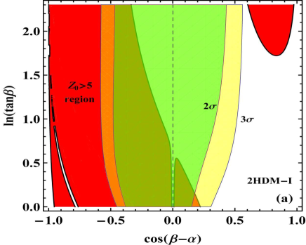
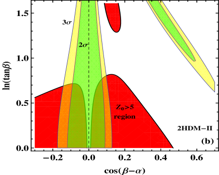
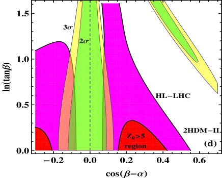
Figure 9: LHC probe of 2HDM parameter space in $\,\cos(\beta\!-\!\alpha)-\tan\beta$  plane. We impose projected sensitivity of the LHC Run-2 by requiring significance$(Z_{0})>5$  for the process $\,pp\!\rightarrow\!H\!\rightarrow\!hh\!\rightarrow\!WW^{*}\gamma\gamma\,$,  with an integrated luminosity ${\cal L}=300\,\text{fb}^{-1}$ at $\sqrt{s}=14$ TeV. All red contours correspond to significance$(Z_{0})=5$  with ${\cal L}=300\,\text{fb}^{-1}$.  Plots (a)-(b) [plots (c)-(d)] present the results for $\,M_{H}=300$ GeV [$M_{H}=400$ GeV], while plots (a) and (c) [plots (b) and (d)] give the results for 2HDM-I [2HDM-II]. In plot-(d), the pink contours ($Z_{0}=5$) show a better probe with ${\cal L}=3\,\text{ab}^{-1}$ at the HL-LHC. The green (yellow) contours present the $2\sigma$ ($3\sigma$) constraints from the Higgs global fit of 2HDM-I [(a) and (c)] and 2HDM-II [(b) and (d)] at the LHC Run-1. In all plots, we have sample inputs $\,(M_{A},\,M_{\!12}^{2})=\left(500\textrm{GeV},\,-(180\textrm{GeV})^{2}\right)\,$,  and the vertical dashed line denotes the alignment limit of the 2HDM.

We combine the significance($Z_{0}$) from both pure leptonic channel $\,WW^{*}\gamma\gamma\rightarrow\ell\bar{\nu}\bar{\ell}\nu\gamma\gamma\,$ and semi-leptonic channel $\,WW^{*}\gamma\gamma\rightarrow q\bar{q}^{\prime}\!\ell\nu\gamma\gamma$  at the LHC Run-2 with 300 fb^-1 integrated luminosity. For this analysis, the relevant mass-parameters of the 2HDM are $\,(M_{H},\,M_{A},\,M_{\!12})\,$.  For demonstration, we will take the sample inputs, $M_{H}=300,400$GeV and $\,(M_{A},\,M_{\!12}^{2})=(500\textrm{GeV},\,-(180\textrm{GeV})^{2})\,$.  With these, we have two remaining parameters in the 2HDM: the mixing angle $\,\alpha\,$ and the VEV ratio $\,\tan\beta\,$.  In Fig. 9, we impose projected sensitivity of the LHC Run-2 by requiring significance$(Z_{0})>5$ .  From this, we derive the red contours in the parameter space of $\cos(\beta\!-\!\alpha)\!-\!\tan\beta$  plane, for 2HDM-I [plots (a) and (c)] and for 2HDM-II [plots (b) and (d)]. The plots (a)-(b) correspond to $\,M_{H}=300$ GeV  and plots (c)-(d) correspond to $\,M_{H}=400$ GeV .  This means that the LHC Run-2 with an integrated luminosity ${\cal L}=300\,\text{fb}^{-1}$ can probe the red contour regions in each plot of Fig. 9 with a significance$(Z_{0})>5$ .  It gives a discovery of the heavier Higgs boson $H$ (with 300 GeV or 400 GeV mass) in the red regions of the 2HDM parameter space.

In Fig. 9, we further present the global fit for the lighter Higgs $h$ (125GeV) by using existing ATLAS and CMS Run-1 data, where the $2\,\sigma$ and $3\,\sigma$ contours of the allowed parameter space are shown by the green and yellow shaded regions, respectively. As we checked, our LHC global fit of the 2HDM is consistent with those in the literature [36]. From this fit, we see that the parameter space favored by the current global fit is around the alignment limit of 2HDM with $\,|\cos(\beta\!-\!\alpha)|\lesssim 0.55\,$ for 2HDM-I and $\,|\cos(\beta\!-\!\alpha)|\lesssim 0.15\,$ for 2HDM-II. But, 2HDM-II still has an extra relatively narrow parameter region starting from $\,\tan\beta\gtrsim 2$ .

Fig. 9(a) has input $\,M_{H}=300$ GeV for 2HDM-I. In this plot, the $\,Z_{0}>5$  region overlaps a large portion of the parameter space favored by the current LHC global fit. But, in Fig. 9(b) for 2HDM-II, the situation is different because the overlap becomes smaller in the region $\,\cos(\beta\!-\!\alpha)<0\,$,  and gets enlarged for $\,\cos(\beta\!-\!\alpha)>0\,$.  For the case of $\,M_{H}=400$ GeV in Fig. 9(c), the probed parameter space of 2HDM-I has sizable reduction, especially for the region of $\,\cos(\beta\!-\!\alpha)\gtrsim-0.05\,$,  in comparison with Fig. 9(a) of $\,M_{H}=300$ GeV .  This is because the signal rate decreases as $\,H\,$ becomes heavier [cf. Fig. 4(a)]. On the other hand, for 2HDM-II, Fig. 9(d) shows that the $\,Z_{0}>5$  contours significantly shrink for $\,M_{H}=400$ GeV.  This is because the signal rate for 2HDM-II drops more rapidly as Higgs mass rises to $\,M_{H}=400$ GeV in the small $\,\tan\beta$  region [cf. Fig. 4(b)]. In this case, we see that the LHC Run-2 with $\,300\,\text{fb}^{-1}$ integrated luminosity has rather weak sensitivities to the parameter space (shown by red contours), and the red contours no longer overlap with the favored region by the current LHC global fit (yellow and green contours). We further analyze the probe from the upcoming High Luminosity LHC (HL-LHC) with $\,3\,\text{ab}^{-1}$ integrated luminosity. We find that the HL-LHC can significantly extend the discovery reach of the parameter space of 2HDM-II, as demonstrated by the pink contour regions ($Z_{0}>5$) of Fig. 9(d).

5 Conclusion

After the LHC discovery of a light Higgs boson $h^{0}$(125GeV) at Run-1, searching for new heavier Higgs state(s) has become a pressing task of the LHC Run-2. Such heavier Higgs state(s) exists in all extended Higgs sectors and can unambiguously point to new physics beyond the standard model (SM).

In this work, we systematically studied the heavier Higgs boson $\,H^{0}\,$ production with the new decay channel, $\,pp\!\rightarrow\!H\!\rightarrow\!hh\!\rightarrow\!WW^{*}\gamma\gamma\,$,  at the LHC Run-2. In section 2, we first analyzed the parameter space of the 2HDM type-I and type-II, including the $Hhh$ cubic Higgs coupling (Fig. 1). We computed the decay branching fractions and production cross section of the heavier Higgs boson $\,H\,$ at the LHC Run-2 over mass range $\,M_{H}=250-600\,$GeV,  as shown in Fig. 2–4. Then, in section 3, we analyzed both pure leptonic mode $\,WW^{*}\!\rightarrow\ell\bar{\nu}\,\bar{\ell}\nu\,$ and semi-leptonic mode $\,WW^{*}\rightarrow q\bar{q}^{\prime}\ell\nu\,$.  This channel has much cleaner backgrounds than the other process $\,pp\!\rightarrow\!H\!\rightarrow\!hh\!\rightarrow\!b\bar{b}\gamma\gamma\,$.  We computed signal and background events using MadGraph5(MadEvent). We applied Pythia to simulate hadronization of partons and adopted Delphes for detector simulations. We followed the ATLAS procedure for event selections and built kinematical cuts to efficiently suppress the SM backgrounds. We analyzed various kinematical distributions for pure leptonic and semi-leptonic decay channels in Fig. 6 and Figs. 7–8 for three sample inputs of Higgs mass $\,M_{H}=(300,\,400,\,600)\,$GeV, respectively. In Table 2–4, we presented the signal and background rates of both channels under the kinematical cuts. In section 4, we combined the significance of pure leptonic and semi-leptonic channels, and analyzed the LHC Run-2 discovery reach of $\,H\,$ as a probe of the parameter space in 2HDM-I and 2HDM-II (Fig. 9). For comparison, we further presented the current Higgs global fit of the LHC Run-1 data in the same plots. Finally, we note that it is hard to detect $H$ with mass above 600 GeV at the LHC (14TeV) runs via di-Higgs production channel. We find it valuable to extend our present LHC study to the future high energy circular colliders $pp$($50\!-\!100$TeV) [37], which are expected to further probe the heavier Higgs boson $H$ with mass up to $O(1\!-\!5)$ TeV range via $\,pp\rightarrow H\rightarrow hh\,$ production channel.

Acknowledgments
We thank Weiming Yao for valuable discussions. We also thank John Ellis, Yun Jiang, Tao Liu and Hao Zhang for useful discussions. LCL and HJH are supported in part by National NSF of China (under grants Nos. 11275101 and 11135003) and National Basic Research Program (under grant No. 2010CB833000). HJH acknowledges the support of visiting grants of IAS Princeton and Harvard University during the finalization of this paper. CD, YQF and HJZ are supported in part by Thousand Talents Program (under Grant No. Y25155AOU1). This work is supported in part by the CAS Center for Excellence in Particle Physics (CCEPP).

References

- [1] G. Aad et al., [ATLAS Collaboration], Phys. Lett. B 716 (2012) 1 [arXiv:1207.7214 [hep-ex]];
- [2] S. Chatrchyan et al., [CMS Collaboration], Phys. Lett. B 716 (2012) 30 [arXiv:1207.7235 [hep-ex]].
- [3] For a review, e.g., J. F. Gunion, H. E. Haber, G. L. Kane and S. Dawson, Front. Phys. 80 (2000) 1; and references therein.
- [4] For a review, e.g., A. Djouadi, Phys. Rept. 459 (2008) 1 [arXiv:hep-ph/0503173]; and references therein.
- [5] For a review, e.g., U. Ellwanger, C. Hugonie, A. M. Teixeira, Phys. Rept. 496 (2010) 1 [arXiv:0910.1785 [hep-ph]]; and references therein.
- [6] For recent studies of minimal gauge extensions with two Higgs doublets (including di-Higgs decay channel ), X.-F. Wang, C. Du, and H.-J. He, Phys. Lett. B 723 (2013) 314 [arXiv:1304.2257]; T. Abe, N. Chen, H.-J. He, JHEP 1301 (2013) 082 [arXiv:1207.4103]; and references therein.
- [7] For a review, e.g., P. Langacker, Rev. Mod. Phys. 81 (2009) 1199 [arXiv:0801.1345]; and references therein.
- [8] R. N. Mohapatra and J. C. Pati, Phys. Rev. D 11 (1975) 566; G. Senjanovic and R. N. Mohapatra, Phys. Rev. D 12 (1975) 1502.
- [9] G. C. Branco, P. M. Ferreira, L. Lavoura, M. N. Rebelo, M. Sher, and J. P. Silva, Phys. Rept. 516 (2012) 1 [arXiv:1106.0034 [hep-ph]]; and references therein.
- [10] E.g., M. Bowen, Y. Cui and J. D. Wells, JHEP 0703 (2007) 036 [arXiv:hep-ph/0701035]; M. J. Dolan, C. Englert and M. Spannowsky, Phys. Rev. 87 (2012) 055002 [arXiv:1210.8166 [hep-ph]]; N. Craig, J. Galloway and S. Thomas, arXiv:1305.2424 [hep-ph]; J. Liu, X. P. Wang and S. h. Zhu, arXiv:1310.3634 [hep-ph]; B. Dumont, J. F. Gunion, Yun Jiang, and S. Kraml, Phys. Rev. D 90 (2014) 035021 [arXiv:1405.3584 [hep-ph]] and arXiv:1409.4088 [hep-ph]; B. Bhattacherjee, A. Chakraborty, and A. Choudhury, arXiv:1504.04308 [hep-ph]; J. Bernon, J. F. Gunion, H. E. Haber, Y. Jiang, and S. Kraml, Phys. Rev. D92 (2015) 075004 [arXiv:1507.00933 [hep-ph]]; and references therein.
- [11] The di-Higgs production channel is also important for probing the light Higgs self-interaction , e.g., J. Baglio, A. Djouadi, R. Grober, M. M. Muhlleitner, J. Quevillon, M. Spira, JHEP 1304 (2013) 151 [arXiv:1212.5581 [hep-ph]]; Weiming Yao, arXiv:1308.6302 [hep-ph], in the Proceedings of Snowmass Community Summer Study (CSS 2013), Snowmass on the Mississippi, July 29–August 6, 2013, Minneapolis, MN, USA; A. J. Barr, M. J. Dolan, C. Englert, D. E. Ferreira de Lima, M. Spannowsky, JHEP 1502 (2015) 016 [arXiv:1412.7154 [hep-ph]]; H.-J. He, J. Ren, and W. Yao, Phys. Rev. D 93 (2015) 015003 [arXiv:1506.03302]; and references therein.
- [12] G. Aad et al. [ATLAS Collaboration], Phys. Rev. Lett. 114 (2015) 081802 [arXiv:1406.5053 [hep-ex]].
- [13] CMS Collaboration, CMS-PAS-HIG-13-025 and CMS-PAS-HIG-13-032.
- [14] N. Chen, C. Du, Y. Fang, and L. C. Lü, Phys. Rev. D 89 (2014) 115006.
- [15] V. Martin-Lozano, J. M. Moreno, C. B. Park, arXiv:1501.03799 [hep-ph].
- [16] G. Funk, D. O’Neil and R. M. Winters, Int. J. Mod. Phys. A 27 (2012) 1250021 [arXiv:1110.3812 [hep-ph]].
- [17] N. Chakrabarty, U. K. Dey and B. Mukhopadhyaya, JHEP 1412 (2014) 166 [arXiv:1407.2145 [hep-ph]].
- [18] A. Djouadi, Phys. Rept. 457 (2008) 1 [hep-ph/0503172].
- [19] S. Dittmaier et al., [LHC Higgs Cross Section Working Group], arXiv:1101.0593 [hep-ph]; S. Heinemeyer et al., [LHC Higgs Cross Section Working Group], arXiv:1307.1347 [hep-ph]; and references therein.
- [20] J. Bernon, J. F. Gunion, H. E. Haber, Yun Jiang, and S. Kraml, Phys. Rev. D 92 (2015) 075004 [arXiv:1507.00933 [hep-ph]].
- [21] J. Alwall, R. Frederix, S. Frixione, V. Hirschi, F. Maltoni, O. Mattelaer, H. S. Shao and T. Stelzer, et al., JHEP 1407 (2014) 079 [arXiv:1405.0301 [hep-ph]].
- [22] A. Alloul, N. D. Christensen, C. Degrande, C. Duhr and B. Fuks, Comput. Phys. Commun. 185 (2014) 2250 [arXiv:1310.1921 [hep-ph]].
- [23] T. Sjostrand, S. Mrenna and P. Z. Skands, JHEP 0605 (2006) 026 [arXiv:hep-ph/0603175].
- [24] J. de Favereau et al., [DELPHES 3 Collaboration], JHEP 1402 (2014) 057 [arXiv:1307.6346 [hep-ex]].
- [25] J. Beringer et al., [Particle Data Group Collaboration], Phys. Rev. D 86 (2012) 010001.
- [26] ATLAS Collaboration, ATLAS-CONF-2013-012, March 5, 2013.
- [27] G. Aad et al., [ATLAS Collaboration], CERN-OPEN-2008-020 and arXiv:0901.0512 [hep-ex].
-
[28]
J. Adelman, A. Loginov, P. Tipton and J. Vasquez,
arXiv:1310.1132 [hep-ex];
S. Dittmaier et al. [LHC Higgs Cross Section Working Group Collaboration], arXiv:1101.0593 [hep-ph]. - [29] ATLAS Collaboration, ATL-PHYS-PUB-2015-022.
- [30] D. Y. Shao, C. S. Li, H. T. Li and J. Wang, JHEP 1307 (2013) 169 [arXiv:1301.1245 [hep-ph]].
- [31] V. Barger, L. L. Everett, C. B. Jackson, A. D. Peterson, G. Shaughnessy, Phys. Rev. Lett. 114 (2015) 011801 [arXiv:1408.0003].
- [32] H.-J. He, J. Ren, and W. Yao, Phys. Rev. D 93 (2015) 015003 [arXiv:1506.03302].
- [33] G. Aad et al. [ATLAS Collaboration], arXiv:0901.0512 [hep-ex].
- [34] G. Cowan, K. Cranmer, E. Gross, and O. Vitells, Eur. Phys. J. C 71 (2011) 1554 [arXiv:1007.1727 [physics.data-an]].
- [35] J. Chang, K. Cheung, J. S. Lee and C. T. Lu, JHEP 1405 (2014) 062 [arXiv:1403.2053 [hep-ph]]; F. Demartin, F. Maltoni, K. Mawatari and M. Zaro, Eur. Phys. J. C 75 (2015) 267 [arXiv:1504.00611 [hep-ph]].
- [36] E.g., A. Djouadi and J. Quevillon, JHEP 1310 (2013) 028 [arXiv:1304.1787 [hep-ph]]; C. Y. Chen, S. Dawson and M. Sher, Phys. Rev. D 88 (2013) 015018 [arXiv:1305.1624 [hep-ph]]; B. Dumont, J. F. Gunion, Yun Jiang, and S. Kraml, Phys. Rev. D 90 (2014) 035021 [arXiv:1405.3584 [hep-ph]]; N. Craig, F. D’Eramo, P. Draper, S. Thomas, H. Zhang, JHEP 1506 (2015) 137 [arXiv:1504.04630 [hep-ph]]; and references therein.
- [37] FCC collaboration, http://tlep.web.cern.ch and M. Bicer et al., JHEP 1401 (2014) 164 [arXiv:1308.6176 [hep-ex]]; CEPC-SPPC collaboration, http://cepc.ihep.ac.cn