Spin canonical rings of log stacky curves

Abstract.

Consider modular forms arising from a finite-area quotient of the upper-half plane by a Fuchsian group. By the classical results of Kodaira–Spencer, this ring of modular forms may be viewed as the log spin canonical ring of a stacky curve. In this paper, we tightly bound the degrees of minimal generators and relations of log spin canonical rings. As a consequence, we obtain a tight bound on the degrees of minimal generators and relations for rings of modular forms of arbitrary integral weight.

1. Introduction

Let $\Gamma$ be a Fuchsian group, i.e.  a discrete subgroup of $\operatorname{PSL}_{2}({\mathbb{R}})$ acting on the upper half plane ${\mathbb{H}}$ by fractional linear transformations, such that $\Gamma\backslash{\mathbb{H}}$ has finite area. We consider the graded ring of modular forms $M(\Gamma)=\bigoplus_{k=0}^{\infty}M_{k}(\Gamma)$. One of the best ways to describe the ring $M(\Gamma)$ is to write down a presentation. To do so, it is useful to have a bound on the degrees in which the generators and relations can occur. In the special case that $\Gamma$ has no odd weight modular forms, Voight and Zureick-Brown give tight bounds [VZB15, Chapters 7-9]. The main theorem of this work extends their result to all Fuchsian groups $\Gamma$.

We can now consider the orbifold $\Gamma\backslash{\mathbb{H}}$ over ${\mathbb{C}}$. For example, in the case $\Gamma$ acts freely on ${\mathbb{H}}$, $\Gamma\backslash{\mathbb{H}}$ is a Riemann surface over ${\mathbb{C}}$. Although $\Gamma\backslash{\mathbb{H}}$ may be non-compact, we can form a compact Riemann surface $\Gamma\backslash{\mathbb{H}}^{*}$ by adding in cusps (with associated divisor of cusps $\Delta$).

In order to find generators and relations for $M(\Gamma)$, we translate the seemingly analytic question of understanding the ring of modular forms into the algebraic category, using a generalization of the GAGA principle. As shown by Voight and Zureick-Brown [VZB15, Proposition 6.1.5], there is an equivalence of categories between orbifold curves and log stacky curves over ${\mathbb{C}}$. For the remainder of the paper, we will work in the algebraic category.

Let $X$ be a smooth proper geometrically-connected algebraic curve of genus $g$ over a field ${\Bbbk}$. It is well known that the canonical sheaf $\Omega_{X},$ with associated canonical divisor $K_{X}$, determines the canonical map $\pi:X\rightarrow{\mathbb{P}}_{\Bbbk}^{g-1}$. Then, the canonical ring is defined to be

$$R(X,K_{X}):=\bigoplus_{d\geq 0}H^{0}(X,dK_{X}),$$

with multiplication structure corresponding to tensor product of sections. In the case that $g\geq 2$, $\Omega_{X}$ is ample and therefore $X\cong\text{Proj }R$. When $g\geq 2$, Petri’s theorem shows that, in most cases, $R(X,K_{X})$ is generated in degree 1 with relations in degree 2 (see Saint-Donat [SD73, p. 157] and Arbarello–Cornalba–Griffiths–Harris [ACGH85, Section 3.3]). This has the pleasant geometric consequence that canonically embedded curves of genus $\geq 4$ which are not hyperelliptic curves, trigonal curves, or plane quintics are scheme-theoretically cut out by degree 2 equations.

Following Voight and Zureick-Brown [VZB15], we generalize Petri’s theorem in the direction of stacky curves equipped with log spin canonical divisors. For a stacky curve $\mathscr{X}$ with coarse space $X$ and stacky points (also called “fractional points”) $P_{1},\ldots,P_{r}$ with stabilizer orders $e_{1},\ldots,e_{r}\in{\mathbb{Z}}_{\geq 2}$, we define

$$\operatorname{Div}\mathscr{X}=\left(\bigoplus_{P\notin\{P_{1},\ldots,P_{r}\}}\langle P\rangle\right)\oplus\left(\bigoplus_{i=1}^{r}\left\langle\frac{1}{e_{i}}P_{i}\right\rangle\right)\subseteq{\mathbb{Q}}\otimes\operatorname{Div}X.$$

Then, a log spin curve is a triple $(\mathscr{X},\Delta,L)$ where $\Delta\in\operatorname{Div}X$ is a log divisor and $L\in\operatorname{Div}\mathscr{X}$ is a log spin canonical divisor, meaning $2L\sim K_{X}+\Delta+\sum_{i=1}^{r}\frac{e_{i}-1}{e_{i}}P_{i}$. The central object of study in this paper is the log spin canonical ring of $(\mathscr{X},\Delta,L),$ defined as

$$R(\mathscr{X},\Delta,L):=\bigoplus_{k\geq 0}H^{0}(X,\lfloor kL\rfloor).$$

A brief overview of stacky curves, log divisors, and log spin canonical rings is given in Subsection  2.1.

Our main theorem is to bound the degrees of generators and relations of a log spin canonical ring. Let $\mathscr{X}$ be a stacky curve with signature $\sigma:=(g;e_{1},\ldots,e_{r};\delta)$. The application of O’Dorney’s work [O’D14, Chapter 5] to log spin canonical rings gives a weak bound in the case $g=0$ in terms of the least common multiples of the $e_{i}$’s. In their treatment of log spin canonical rings, Voight and Zureick-Brown [VZB15, Corollary 10.4.6] bounded generator degrees by $6\cdot\max(e_{1},\ldots,e_{r})$ and relation degrees by $12\cdot\max(e_{1},\ldots,e_{r})$ when $L$ is effective. Note that the bounds we deduce differ from those stated in Voight and Zureick-Brown [VZB15, Corollary 10.4.6] by a factor of 2 because their grading convention differs from ours by a factor of 2.

These bounds are far from tight and do not collectively cover all cases in all genera. The main theorem of this paper gives significantly tighter bounds for the log spin canonical ring of any log spin curve.

Theorem 1.1.

Let $(\mathscr{X},\Delta,L)$ be a log spin curve over a perfect field ${\Bbbk}$, so that $\mathscr{X}$ has signature $\sigma=(g;e_{1},\ldots,e_{r};\delta)$.

Then the log spin canonical ring is generated as a ${\Bbbk}$-algebra by elements of degree at most $e:=\max(5,e_{1},\ldots,e_{r})$ with relations generated in degrees at most $2e$, so long as $\sigma$ does not lie in a finite list of exceptional cases, as given in Table  2 for signatures with $g=1$ and Table  7 for signatures with $g=0$.

Remark 1.2.

In fact, the proof of Theorem  1.1 holds with $\Delta$ replaced by an arbitrary effective divisor of the coarse space. Furthermore, one may relax the assumption that ${\Bbbk}$ is perfect. Instead, one only need assume that the stacky curve is separably rooted, as described further in Remark  2.2.

Theorem  1.1 is proven separately in the cases that the genus $g=0,g=1,$ and $g\geq 2$ in Theorems  7.4,  6.1, and  5.6, respectively. In each of these proofs, we follow a similar inductive process utilizing the lemmas of Section  4; however, in the first two cases we explicitly construct specific base cases and present a finite list of exceptional cases, whereas in the genus $g\geq 2$ case we deduce base cases from more general arguments.

Remark 1.3.

In addition to providing bounds on the degrees of generators and relations of log spin canonical rings, the proof of the genus one and genus zero cases of our main theorem also yield explicit systems of generators and initial ideals of relations, as described in Remarks  6.2 and  7.5. Furthermore, our proof of the genus $g\geq 2$ case provides an inductive procedure for explicitly determining the generators and initial ideal of relations of a log spin canonical ring given a presentation of the corresponding ring on the coarse space, but actually computing such a presentation of log spin canonical on the coarse space can be difficult. Many explicit systems of generators and relations for curves of genus $2\leq g\leq 15$ are detailed in interesting examples by Neves [Nev03, Section III.4].

Remark 1.4.

The explicit construction described in Remark  1.3 also reveals that the bounds given in Theorem  1.1 are tight. In almost all cases, the log spin canonical ring requires a generator in degree $e=\max(5,e_{1},\ldots,e_{r})$ and a relation in degree at least $2e-4$. Furthermore, there are many infinite families of cases which require a generator in degree $e=\max(5,e_{1},\ldots,e_{r})$ and a relation in degree exactly $2e$. For further detail, see Remarks  7.5,  6.2, and  5.7 in the cases that the genus is $0,1,$ or $\geq 2$ respectively.

Combining the main theorem of this paper, Theorem  1.1 with the main theorem from Voight and Zureick-Brown  [VZB15, Theorem 1.4] and a minor Lemma [VZB15, Lemma 10.2.1] we have the following application to rings of modular forms.

Corollary 1.5.

Let $\Gamma$ be a Fuchsian group and $\mathscr{X}$ the stacky curve associated to $\Gamma\backslash{\mathbb{H}}$ with signature $\sigma=(g;e_{1},\ldots,e_{r};\delta)$.

If $M_{k}(\Gamma)=0$ for all odd $k$, then the ring of modular forms $M(\Gamma)$ is generated as a ${\mathbb{C}}$-algebra by elements of degree at most $6\cdot\max(3,e_{1},\ldots,e_{r})$ with relations generated in degrees at most $12\cdot\max(3,e_{1},\ldots,e_{r})$.

If there is some odd $k$ for which $M_{k}(\Gamma)\neq 0$, then the ring of modular forms $M(\Gamma)$ is generated as a ${\mathbb{C}}$-algebra by elements of degree at most $\max(5,e_{1},\ldots,e_{r})$ with relations generated in degree at most $2\cdot\max(5,e_{1},\ldots,e_{r})$ so long as $\sigma$ does not lie in a finite list of exceptional cases which are listed and described in Table  2 for signatures with $g=1$ and in Table  7 for signatures with $g=0$.

Remark 1.6.

If $M(\Gamma)$ has some odd weight modular form, then it has an odd weight modular form in weight $3$. When $g\geq 2$, we see that this is true because $\dim_{\Bbbk}H^{0}(\mathscr{X},3L)>0$ by Riemann–Roch and the fact that $\deg\lfloor 3L\rfloor>2g-1$. When the genus is zero or one, we see that there is a generator in weight $1$ or weight $3$ in the base cases given in Table  1 and Table  4. Hence, there is an odd weight modular form in weight $3$ in general. A consequence of this observation is that the bound on the degree of generators and relations when $M(\Gamma)$ has some odd weight modular form, as given in Corollary  1.5, is closely related to the degree of the minimal odd weight modular form.

Example 1.7.

In this example, we deduce bounds on the weight of generators and relations of the ring of modular forms associated to any congruence subgroup $\Gamma\subset SL_{2}({\mathbb{Z}})$. Since the action of $SL_{2}({\mathbb{Z}})$ on ${\mathbb{H}}$ only has points with stabilizer order 1, 2 and 3, and has at least one cusp, the action of $\Gamma$ on ${\mathbb{H}}$ can only have points with stabilizer order 1, 2 and 3, and has at least one cusp.

If $\Gamma$ has no nonzero odd weight modular forms, then $\Gamma$ is generated in weight at most $6$ with relations in weight at most $12$. This follows from work by Voight and Zureick-Brown [VZB15, Theorem 1.4 and Theorem 9.3.1]. Note that the exceptional cases of their result [VZB15, Theorem 9.3.1], which happen when the genus is zero, do not occur because $\delta>0$.

If $\Gamma$ has some nonzero odd weight modular form, then it must have no points with stabilizer order 2 by Remark  2.10. Therefore, by Corollary  1.5, $M(\Gamma)$ is generated in weight at most $5$ with relations in weight at most $10$. Furthermore, it is not difficult to show that $M(\Gamma)$ is generated in weight at most 4 with relations in weight at most 8 when the genus of the stacky curve associated to $\Gamma\backslash{\mathbb{H}}^{*}$ is 0 or 1, as noted in Remark  7.6. Note that the exceptional cases in Tables  2 and  7 do not occur because $\Gamma$ has a cusp, so $\delta>0$.

Remark 1.8.

In the case that $M_{k}(\Gamma)=0$ for all odd $k$, the generation bound of $6\cdot\max(3,e_{1},\ldots,e_{r})$ and relation bound of $12\cdot\max(3,e_{1},\ldots,e_{r})$ can be reduced to $2\cdot\max(3,e_{1},\ldots,e_{r})$ and $4\cdot\max(3,e_{1},\ldots,e_{r})$, apart from several small families of cases. See  [VZB15, Theorem 9.3.1] and  [VZB15, Theorem 8.7.1] for a more precise statement of these bounds in the cases that $g=0$ and $g>0$ respectively. Note that we multiply all bounds given in Voight and Zureick-Brown [VZB15] by a factor of two. Our grading convention for log spin canonical rings uses weight $k$ for the degree whereas Voight and Zureick-Brown $d=2k$ for degree.

The remainder of the paper will be primarily devoted to proving Theorem  1.1. The idea of the proof will be to induct first on the number of stacky points and then on the stabilizer order of those points. To this end, we first review important background in Section  2; providing essential examples in Section 3; develop various inductive tools in Section  4; and prove Theorem  1.1 in genus $g\geq 2$, genus $g=1$, and genus $g=0$ in Sections  5,  6, and  7 respectively. Finally, in Section  8, we pose several questions for future research.

2. Background

Here we collect various definitions and notation that will be used throughout the paper. For basic references on the statements and definitions used below, see Hartshorne [Har77, Chapter IV], Saint-Donat [SD73], Arbarello–Cornalba–Griffiths–Harris [ACGH85, Section III.2], and Voight–Zureick-Brown [VZB15, Chapter 2, Chapter 5].

For the remainder of this paper, fix an algebraically closed field ${\Bbbk}$. This is no restriction on generality, as generator and relation degrees are preserved under base change to the algebraic closure.

2.1. Stacky Curves and Log Spin Canonical Rings

We begin by setting up the notation for stacky curves and canonical rings. Wherever possible, we opt for a more elementary scheme-theoretic approach, instead of a stack-theoretic one. See Remark  2.2 for more details.

Definition 2.1.

A stacky curve $\mathscr{X}$ over an algebraically closed field ${\Bbbk}$ is the datum of a smooth proper integral scheme $X$ of dimension $1$, together with a finite number of closed points of $X$, $P_{1},\ldots,P_{r}$, called stacky points, with stabilizer orders $e_{1},\ldots,e_{r}\in{\mathbb{Z}}_{\geq 2}.$ The scheme $X$ associated to a stacky curve $\mathscr{X}$ is called the coarse space of $\mathscr{X}$.

Remark 2.2.

Stacky curves may be formally defined in the language of stacks, as is done in the works of Voight and Zureick-Brown [VZB15], Abramovich and Vistoli [AV02], and Behrend and Noohi [BN06].

The results of this paper can be easily phrased in terms of the language of stacks. If one works over an arbitrary field ${\Bbbk}$ (which need not be algebraically closed) one can extend Theorem  1.1 to hold in the case that the stacky curve $\mathscr{X}$ is tame and separably rooted, i.e.  the residue field of each of the stacky points is separable.

With this stack-theoretic description in mind, the remainder of this paper is primarily phrased using the language of schemes.

Definition 2.3.

Let $\mathscr{X}$ be a stacky curve over ${\Bbbk}$ with coarse space $X$ of genus $g$ and stacky points $P_{1},\ldots,P_{r}$ with stabilizer orders $e_{1},\ldots,e_{r}\in{\mathbb{Z}}_{\geq 2}$. Then, we notate

$$\operatorname{Div}\mathscr{X}:=\left(\bigoplus_{P\notin\{P_{1},\ldots,P_{r}\}}\langle P\rangle\right)\oplus\left(\bigoplus_{i=1}^{r}\left\langle\frac{1}{e_{i}}P_{i}\right\rangle\right)\subseteq{\mathbb{Q}}\otimes\operatorname{Div}X.$$

We can equip stacky curves with a log divisor $\Delta$ that is a sum of distinct points each with trivial stabilizer. A divisor $\Delta$ of this form is called a log divisor. We use $\delta:=\deg\Delta$ to refer to the degree of the log divisor. If $\mathscr{X}$ has coarse space $X$ of genus $g$, then we say $\mathscr{X}$ has signature $\sigma=(g;e_{1},\ldots,e_{r};\delta)$.

Definition 2.4.

If divisor $D\in\operatorname{Div}\mathscr{X}$ and $D=\sum_{i=1}^{n}\alpha_{i}P_{i}$ with $\alpha_{i}\in{\mathbb{Q}}$, the floor of a divisor $\lfloor D\rfloor$ is defined to be $\lfloor D\rfloor:=\sum_{i=1}^{n}\lfloor\alpha_{i}\rfloor P_{i}$.

A pair of a stacky curve and a log divisor $(\mathscr{X},\Delta)$ is called a log stacky curve and the study of their canonical rings is the main focus of the work by Voight and Zureick-Brown [VZB15]. For this paper, we consider log spin curves which are triples $(\mathscr{X},\Delta,L)$ where $\mathscr{X}$ is a stacky curve, $\Delta$ is a log divisor, and $L\in\operatorname{Div}\mathscr{X}$ satisfies $2L\sim K_{X}+\Delta+\sum_{i=1}^{r}\frac{e_{i}-1}{e_{i}}P_{i}$. Such a divisor $L$ is called a log spin canonical divisor on $(\mathscr{X},\Delta)$. Throughout the paper, we use the notation $L_{X}:=\lfloor L\rfloor.$ to refer to the log spin canonical divisor (also known as the half-canonical divisor, semi-canonical divisor, or theta characteristic) associated to the coarse space $X$ of $\mathscr{X}.$ (i.e.  $L_{X}$ is a divisor such that $2L_{X}\sim K_{X}+\Delta$). We define $H^{0}$ of a stacky divisor as follows.

Definition 2.5.

Recall the standard notation for the line bundle ${\mathscr{O}}(D)$ on an integral normal scheme $X$ associated to a divisor $D\in\operatorname{Div}X$:

$$\Gamma(U,{\mathscr{O}}(D)):=\{f\in{\Bbbk}(X)^{\times}:\operatorname{Div}|_{U}f+D|_{U}\geq 0\}\cup\{0\}.$$

Let $\mathscr{X}$ be a stacky curve with coarse space $X$. If $D\in\operatorname{Div}\mathscr{X}$ is a Weil divisor, then we define

$$H^{0}(\mathscr{X},D) :=H^{0}(X,\lfloor D\rfloor)$$

$$H^{0}(\mathscr{X},{\mathscr{O}}(D)) :=H^{0}(\mathscr{X},D)$$

$$h^{0}(\mathscr{X},{\mathscr{O}}(D)) :=\dim_{\Bbbk}H^{0}(\mathscr{X},{\mathscr{O}}(D))$$

If $R$ is a graded ring, then we let $(R)_{k}$ refer to the $k^{\text{th}}$ graded component of $R$.

Remark 2.6.

The log canonical ring, defined to be the direct sum of the even graded pieces of the log spin canonical ring, is Gorenstein. It is Cohen–Macaulay from [Wat81, Example 2.5(a)] and then Gorenstein by [Wat81, Corollary 2.9]. In particular, this tells us that a log spin canonical curve, the projectivization of a log spin canonical ring, is projectively Gorenstein.

Remark 2.7.

Although Definition  2.5 may seem fairly ad hoc, it is naturally motivated in the context of stacks. See Voight and Zureick-Brown [VZB15, Lemma 5.4.7] for a proof that Definition  2.5 is equivalent to the stack-theoretic description.

Definition 2.8.

Let $D\in\operatorname{Div}\mathscr{X}.$ If $z\neq 0$ is a rational section of ${\mathscr{O}}(D)$ denote the order of zero of $z$ at $P$ by $\operatorname{ord}_{P}^{D}(z)$.

Definition 2.9.

The log spin canonical ring of $(\mathscr{X},\Delta,L)$ is

$$R(\mathscr{X},\Delta,L):=\bigoplus_{k\geq 0}H^{0}(\mathscr{X},kL).$$

When the log spin curve is fixed, we usually use $R$ or $R_{L}$ to represent $R(\mathscr{X},\Delta,L)$.

Remark 2.10.

Suppose $(\mathscr{X},\Delta,L)$ is a log spin curve. Note that $L$ is of the form

$$L=\sum_{i=1}^{r}\frac{{e_{i}}-1}{2{e_{i}}}P_{i}+\sum_{i=1}^{s}a_{i}Q_{i}$$

where $a_{i}\in{\mathbb{Z}}$ and $e_{i}$ are odd. This is due to the fact that $L\in\operatorname{Div}\mathscr{X}$: if some $e_{i}$ were even, then $\frac{e_{i}-1}{2e_{i}}$ would be in reduced form implying $L\notin\operatorname{Div}\mathscr{X}$.

Remark 2.11.

Except in degenerate cases, such as when the signature is $(0;3,3,3;0)$ as covered in the first line of Table  7, we have the following important restriction on the generators of $R_{L}$. For each $e_{i}$ in the signature of $\mathscr{X}$, there will be at least one generator with degree $0\bmod e_{i}$ and at least one generator with degree $-2\bmod e_{i}$. Although this is an important restriction on the generators, we will not use this in the remainder of the paper.

Remark 2.12.

Suppose $(\mathscr{X},\Delta,L)$ is a log spin curve. Note that $\deg\Delta$ is even. because $2\cdot\deg L=\deg\Delta+\deg\lfloor K\rfloor=\deg\Delta+2(g-1).$ In particular, we shall often use $\deg\Delta\neq 1$.

2.2. Saturation

We define the notion of the saturation of a divisor, as can be found in Voight and Zureick-Brown  [VZB15, Section 7.2]. The classification of the saturations of log spin canonical divisors are used in the proof of the main theorem and the various lemmas in Section  4.

Definition 2.13.

Let $D$ be a divisor on $\mathscr{X}$. The effective monoid of $D$ is the monoid

$$\operatorname{Eff}(D):=\{k\in{\mathbb{Z}}_{\geq 0}:\deg\lfloor kD\rfloor\geq 0\}.$$

Definition 2.14.

The saturation of a monoid $M\subseteq{\mathbb{Z}}_{\geq 0}$, denoted $\operatorname{sat}(M)$, is the smallest integer $s$ such that $M\supseteq{\mathbb{Z}}_{\geq s}$, if such an integer exists.

Remark 2.15.

For $D\in\operatorname{Div}\mathscr{X}$, we will often call $\operatorname{sat}(\operatorname{Eff}(D))$ the saturation of a divisor $D$. For examples, see Subsection  7.1.

2.3. Monomial Ordering

Here we give a brief overview of the three monomial orderings that we use. For further reference on monomial orderings, initial ideals, and Gröbner bases, see Eisenbud [Eis95, Section 15.9] and Cox–Little–O’Shea [CLO07, Chapter 2].

Definition 2.16.

Let ${\Bbbk}[x_{1}$, $\ldots$, $x_{n}]$ be a graded polynomial ring with $\deg x_{i}=k_{i}$ and let $\alpha:=\prod_{i=1}^{n}x_{i}^{f_{i}}\in{\Bbbk}[x_{1}$, $\ldots$, $x_{n}]$ be a monomial. Then we define the degree of $\alpha$ to be

$$\deg\alpha:=\sum_{i=1}^{n}k_{i}f_{i}.$$

Definition 2.17.

The graded reverse lexicographic order, or grevlex $\prec_{\text{grevlex}}$ is defined as follows. If $\alpha:=\prod_{i=1}^{n}x_{i}^{f_{i}}$ and $\beta:=\prod_{i=1}^{n}x_{i}^{f_{i}^{\prime}}$ are monomials in ${\Bbbk}[x_{1}$, $\ldots$, $x_{n}]$, then $\alpha\succ_{\text{grevlex}}\beta$ if either

(2.1) $$\deg\alpha=\sum_{i=1}^{n}k_{i}f_{i}>\sum_{i=1}^{n}k_{i}f_{i}^{\prime}=\deg\beta$$

or

(2.2) $$\deg\alpha=\deg\beta\text{ and }f_{i}<f_{i}^{\prime}\text{ for the largest }i\text{ such that }f_{i}\neq f_{i}^{\prime}.$$

Remark 2.18.

Note that the ordering of the variables matters in Equation  2.2.

Our inductive arguments in Section  4 will usually have an inclusion $R\supseteq R^{\prime}$ of log spin canonical rings such that $R_{L}$ is generated by elements $x_{i}$ and $R$ is generated over $R_{L^{\prime}}$ by elements $y_{j}$. In these cases, it is natural to consider term orders which treat these sets of variables separately.

Definition 2.19.

The block term order is defined as follows. Let ${\Bbbk}[y_{1},\ldots,y_{m}]$ and ${\Bbbk}[x_{1},\ldots,x_{n}]$ be weighted polynomial rings with $\deg y_{i}=c_{i},\>\deg x_{i}=k_{i}.$ Further assume we are given existing term orders $\prec_{y}$ and $\prec_{x}$. Let $\alpha:=\prod_{j=1}^{m}y_{j}^{h_{i}}$ $\prod_{i=1}^{n}x_{i}^{f_{i}}$ and $\beta:=\prod_{j=1}^{m}y_{j}^{h_{i}^{\prime}}\prod_{i=1}^{n}x_{i}^{f_{i}^{\prime}}$ be monomials in ${\Bbbk}[y_{1},\ldots,y_{m}]\otimes$ ${\Bbbk}[x_{1},\ldots,x_{n}]$. Let $\alpha_{y}:=\prod_{j=1}^{m}y_{j}^{h_{i}}$ be the part of $\alpha$ in ${\Bbbk}[y_{1},\ldots,y_{m}]$ and likewise with $\alpha_{x}$, $\beta_{y}$, and $\beta_{x}$.

In the (graded) block (or elimination) term ordering on ${\Bbbk}[y_{k_{1}^{\prime},1},\ldots,y_{k_{m}^{\prime},m}]\otimes{\Bbbk}[x_{k_{1},1},\ldots,x_{k_{n},n}]$, we define $\alpha\succ\beta$ if

1. $\deg\alpha>\deg\beta$ or

2. $\deg\alpha=\deg\beta$ and $\alpha_{y}\succ_{y}\beta_{y}$ or

3. $\deg\alpha=\deg\beta$ and $\alpha_{y}=\beta_{y}$ and $\alpha_{x}\succ_{x}\beta_{x}$.

Now we give brief definitions of initial terms and Gröbner bases. These will be used in the proofs of the inductive lemmas in Section  4 as well as in the proof of Theorem  1.1.

Definition 2.20.

Let $\prec$ be an ordering on ${\Bbbk}[x_{1}$, $\ldots$, $x_{n}]$, with $\deg x_{i}=k_{i}$, and let $f\in{\Bbbk}[x_{1},\ldots,x_{n}]$ be a homogeneous polynomial. The initial term $\operatorname{in_{\prec}}(f)$ of $f$ is the largest monomial in the support of $f$ with respect to the ordering $\prec$. Furthermore, we set $\operatorname{in_{\prec}}(0):=0$.

Definition 2.21.

Let $I$ be a homogeneous ideal of ${\Bbbk}[x_{1}$, $\ldots$, $x_{n}]$. Then the initial ideal $\operatorname{in_{\prec}}(I)$ of $I$ is the ideal generated by the initial terms of homogeneous polynomials in $I$:

$$\operatorname{in_{\prec}}(I):=\langle\operatorname{in_{\prec}}(f)\rangle_{f\in I}$$

Definition 2.22.

Let $I$ be a homogeneous ideal of ${\Bbbk}[x_{1}$, $\ldots$, $x_{n}]$. A Gröbner basis for $I$, also known as a standard basis for $I$, is a set of elements in $I$ such that their initial terms generate the initial ideal of $I$.

3. Examples

In this section, we work out several examples of computing presentations for spin canonical rings. In addition to providing intuition for the lemmas of Section  4, these examples also serve as useful base cases for our inductive proof of Theorem  1.1.

Example 3.1.

Let $(\mathscr{X}^{\prime},0,L^{\prime})$ be a log spin curve of genus $g=1,$ with $L^{\prime}=0$. Counting dimensions, we see $h^{0}(\mathscr{X},kL^{\prime})=1$ for all $k\in\mathbb{Z}_{\geq 0}$ so it is immediately clear that $R_{L^{\prime}}\cong{\Bbbk}[x]$ with $x$ a generator in degree 1.

Remark 3.2.

In the following examples, in order to find the Hilbert series of a stacky curve, we will cite [Zho11, Theorem 4.2.1]. Note that [BRZ13, Theorem 3.1] restates [Zho11, Theorem 4.2.1] with the restriction that the dimension of the orbifold (which is the same as a stacky curve in dimension 1, by [VZB15, Proposition 6.1.5],) is strictly more than 1. The statement holds equally well when the dimension is $1$, but this restriction is included in [BRZ13, Theorem 3.1] because in birational geometry “orbifolds” usually refer to a normal variety ramified only in codimension at least 2, while the stacky points we are dealing with appear in codimension 1.

Example 3.3.

Let $(\mathscr{X},3\cdot\infty,L)$ be a stacky curve with coarse space $X$ and signature $(0;3;3)$. Let $P_{1}$ denote the lone stacky point which has stabilizer order $3$ and suppose $\infty$ is a fixed closed point of $X$ that is not equal to $P_{1}$.

Recall the notation $L_{X}=\lfloor L\rfloor\in\operatorname{Div}X$ (i.e.  the divisor without any stacky points). We will deduce the structure of the log spin canonical ring $R_{L}$ from the structure of the spin canonical ring $R_{L_{X}}:=R(X,3\cdot\infty,L_{X})$. This technique will later be generalized in Lemma  4.4.

Note that $R_{L_{X}}\cong{\Bbbk}[x_{1},x_{2}]$ where $\deg x_{1}=\deg x_{2}=1.$ To see this, observe that we will need two generators in degree $1$ because $h^{0}(X,L_{X})=2$ by Riemann–Roch. Because $L_{X}$ is very ample, we have that $R_{L_{X}}$ is generated in degree 1. To conclude, note that $R_{L_{X}}$ does not have any relations. If there exists some relation, then $\dim\text{Proj }R_{L_{X}}<1$. This would contradict the fact that $L_{X}$ is very ample. Thus, $\text{Proj }R_{L_{X}}\cong X$ which has dimension 1.

Next, we construct generators and relations for $R_{L}$ using those of $R_{L_{X}}$. Note that we have a natural inclusion $\iota:R_{L_{X}}\hookrightarrow R_{L}$ induced by the inclusions $H^{0}(\mathscr{X},kL_{X})\hookrightarrow H^{0}(\mathscr{X},kL)$ for each $k\geq 0$. By Riemann–Roch, we see there is some element $y_{1,3}\in(R_{L})_{3}$ with $\operatorname{ord}_{P_{1}}(y_{1,3})=-1$, not in the image of the inclusion $\iota$. We claim that there exist $a_{1},a_{2}\in{\Bbbk}$ and a degree $4$ polynomial $f(x_{1},x_{2})\in{\Bbbk}[x_{1},x_{2}]$ such that

$$R_{L}\cong{\Bbbk}[x_{1},x_{2},y_{1,3}]/(a_{1}x_{1}y_{1,3}+a_{2}x_{2}y_{1,3}+f(x_{1},x_{2}))$$

First, note that $x_{1},x_{2},y_{1,3}$ generate all of $R_{L}$ from the Generalized Max Noether Theorem for genus zero curves from Voight and Zureick-Brown [VZB15, Lemma 3.1.1]. That is, the maps

$$H^{0}(\mathscr{X},3L)\otimes H^{0}(\mathscr{X},(k-3)L)\rightarrow H^{0}(\mathscr{X},kL)$$

are surjective for $k\geq 4$. A relation of the form $a_{1}x_{1}y_{1,3}+a_{2}x_{2}y_{1,3}+f(x_{1},x_{2})=0$ must exist because $h^{0}(\mathscr{X},4L)-h^{0}(\mathscr{X},4L_{X})=1,$ but $x_{1}y_{1,3}$ and $x_{2}y_{1,3}$ define two linearly independent elements with nontrivial image in the 1-dimensional vector space $H^{0}(\mathscr{X},4L)/H^{0}(\mathscr{X},4L_{X}).$ So, we obtain a surjection

(3.1) $${\Bbbk}[x_{1},x_{2},y_{1,3}]/(a_{1}x_{1}y_{1,3}+a_{2}x_{2}y_{1,3}+f(x_{1},x_{2}))\rightarrow R_{L}.$$

To complete the example, it suffices to show there are no additional relations. One method would be to use [Zho11, Theorem 4.2.1] to write down the Hilbert series and then check this agrees with the Hilbert series of the ring we constructed above. Here is an alternative method: First, note that $a_{1}x_{1}y_{1,3}+a_{2}x_{2}y_{1,3}+f(x_{1},x_{2})$ is irreducible because there are no relations among $x_{1},x_{2}$ and $y_{1,3}$ in lower degrees. Hence, ${\Bbbk}[x_{1},x_{2},y_{1,3}]/(a_{1}x_{1}y_{1,3}+a_{2}x_{2}y_{1,3}+f(x_{1},x_{2}))$ is integral and is 2-dimensional. Thus, the map (3.1) defines a surjection from an integral 2-dimensional ring to a 2-dimensional ring. Therefore, it is an isomorphism.

Example 3.4.

Let $(\mathscr{X}^{\prime},0,L^{\prime})$ be a log spin curve with signature $\sigma=(0;3,7,7;0)$ and $L^{\prime}\sim-\infty+\frac{1}{3}P_{1}+\frac{3}{7}P_{2}+\frac{3}{7}P_{3},$ where $P_{1},P_{2},$ and $P_{3}$ are distinct points. In this example, we will exhibit a minimal presentation for $R^{\prime}=R(\mathscr{X}^{\prime},0,L^{\prime})$ and show that $R^{\prime}$ is generated as a ${\Bbbk}$-algebra in degrees up to $e:=\max(5,3,7,7)=7$ with relations generated in degrees up to $2e=14$. Notice that $\deg\lfloor kK_{\mathscr{X}^{\prime}}\rfloor=-k+\lfloor\frac{k}{3}\rfloor+2\lfloor\frac{3k}{7}\rfloor$.

First, by [Zho11, Theorem 4.2.1], the Hilbert series of this log spin curve is

$$P_{(\mathscr{X}^{\prime},0,L^{\prime})}(k) =\frac{1-2k+k^{2}-2k^{3}+k^{4}}{(1-k)^{2}}+\frac{k^{3}}{(1-k)(1-k^{3})}+2\frac{k^{3}+k^{5}+k^{7}}{(1-k)(1-k^{7})}.$$

For $k=0,1,2,\ldots$ we have

$$P_{(\mathscr{X}^{\prime},0,L^{\prime})}(k)=1,0,0,1,0,1,1,2,1,1,2,1,3,2,3,\ldots$$

so $R^{\prime}$ must have some generators $x_{3,1},x_{5,1},x_{7,1},x_{7,2}$ with $x_{i,j}\in H^{0}(\mathscr{X}^{\prime},iL^{\prime})$.

By the Generalized Max Noether Theorem for genus 0 curves (see Voight and Zureick-Brown [VZB15, Lemma 3.1.1]),

(3.2) $$H^{0}(\mathscr{X}^{\prime},21\cdot L^{\prime})\otimes H^{0}(\mathscr{X}^{\prime},(k-21)L^{\prime})\rightarrow H^{0}(\mathscr{X}^{\prime},kL^{\prime})$$

is surjective whenever $\deg(\lfloor(k-21)L^{\prime}\rfloor)\geq 0$. It is fairly easy to see, by use of Riemann–Roch, that the saturation of $L^{\prime}$ is $5$ (see Definition  2.14). Then the map in  (3.2) is surjective when $k\geq 21+s=26$ (i.e.  $R^{\prime}$ is generated up to degree 25).

To show that these generate all of $R^{\prime}$, we need to show that all $H^{0}(\mathscr{X}^{\prime},kL^{\prime})$ are generated by lower degrees for $k=6$ and $7<k\leq 25$. This can be seen by checking these remaining cases via pole degree considerations or using the generalized Max Noether’s theorem. Thus, $R^{\prime}$ is generated in degrees $\{3,5,7,7\}$.

By relabelling the variables if necessary, we can assume that $x_{7,1}$ corresponds to the generator with maximal pole order at $P_{2}$ and $x_{7,2}$ correspond to the generator with maximal pole order at $P_{3}$. We then have two relations

$$a_{1}x_{5,1}^{2}+a_{2}x_{7,2}x_{3,1}+a_{3}x_{7,1}x_{3,1}=0 10$$ in degree

$$b_{1}x_{7,2}^{2}+b_{2}x_{7,2}x_{7,1}+b_{3}x_{7,1}^{2}+b_{4}x_{5,1}x_{3,1}^{3}=0 14$$ in degree .

Note that $a_{1}$ and $b_{1}$ are both nonzero. For example, if $a_{1}=0$, we would have

$$a_{2}x_{7,2}x_{3,1}=-a_{3}x_{7,1}x_{3,1}$$

implying that $a_{2}=a_{3}=0$, which would mean there is no relation at all. A similar pole order consideration in forcing $b_{1}$ to be nonzero.

Let $I$ be the ideal generated by these relations in ${\Bbbk}[x_{7,2},x_{7,1},x_{5,1},x_{3,1}]$. Under grevlex with $x_{3,1}\prec x_{5,1}\prec x_{7,1}\prec x_{7,2}$, the initial ideal of $I$ is

$$\operatorname{in_{\prec}}(I)=\langle x_{7,2}^{2},x_{5,1}^{2}\rangle$$

since $a_{1}$ and $b_{1}$ are nonzero. Since this ring has Hilbert series equal to $P_{(\mathscr{X}^{\prime},0,L^{\prime})}(k)$, we have found all the relations.

Therefore, the canonical ring $R^{\prime}$ has presentation $R^{\prime}={\Bbbk}[x_{7,2},x_{7,1},x_{5,1},x_{3,1}]/I$ with initial ideal $\operatorname{in_{\prec}}(I)$ generated by quadratics under grevlex with $x_{3,1}\prec x_{5,1}\prec x_{7,1}\prec x_{7,2}$. Thus, $R^{\prime}$ is generated up to degree $e=7$ with relations up to degree $2e=14$, as desired.

Example 3.5.

Let $(\mathscr{X}^{\prime},0,L^{\prime})$ be a log spin curve of genus $1$ with $L^{\prime}=P-Q+\frac{1}{3}P_{1}+\frac{1}{3}P_{2}$. In this example, we show that

$$R_{L^{\prime}}\cong{\Bbbk}[u,x_{3},y_{3},y_{4}]/(x_{3}y_{3}-\alpha uy_{4},y_{4}^{2}-\beta x_{3}^{2}u-\gamma y_{3}^{2}u).$$

Let $u\in H^{0}(\mathscr{X},2L^{\prime})$ be any nonzero element, let $x_{3}\in H^{0}(\mathscr{X},3L^{\prime})$ be an element with a pole at $P_{1}$ but not at $P_{2}$ and $y_{3}\in H^{0}(\mathscr{X},3L^{\prime})$ be an element with a pole at $P_{2}$ but not at $P_{1}$. Let $y_{4}\in H^{0}(\mathscr{X},4L^{\prime})$ be an element with a pole of order 1 at both $P_{1}$ and $P_{2}$. Note that $x_{3}$ and $y_{3}$ exist because the linear systems $3P-3Q\sim P-Q$, $3P-3Q+P_{1}$, and $3P-3Q+P_{1}+P_{2}$ are 0, 1, and 2 dimensional respectively.

Then, there exist constants $\alpha,\beta,\gamma\in{\Bbbk}$ so that $R_{L^{\prime}}\cong{\Bbbk}[u,x,y_{3},y_{4}]/(xy_{3}-\alpha uy_{4},y_{4}^{2}-\beta x^{2}u-\gamma y^{2}u).$ The proof of this is fairly algorithmic: We may first write down the Hilbert series of $(R_{L^{\prime}})_{n}$ over ${\Bbbk}$ using [Zho11, Theorem 4.2.1], then verify that these generators and relations produce the correct number of independent functions via an analysis of zero and pole order. The details are omitted as it is analogous to Example  3.4.

Example 3.6.

Let $(\mathscr{X}^{\prime},0,L^{\prime})$ be a log spin curve of genus 1 with $L^{\prime}=P-Q+\frac{2}{5}P_{1}.$ Let $x_{2}\in(R_{L})_{2}$ be any nonzero element. We obtain $\operatorname{Div}x_{2}|_{P_{1}}=0,$ since $2P-2Q\sim 0$ and by Riemann–Roch, $\dim_{\Bbbk}(P_{L})_{2}=1.$ Let $y_{3}\in(R_{L})_{3}$ be any nonzero element. We obtain $\operatorname{Div}y_{3}|_{P_{1}}=-P_{1},$ by Riemann–Roch, since if $y_{3}$ did not have a pole at $R$, we would obtain $y_{3}\in H^{0}(\mathscr{X},3P-3Q)\cong H^{0}(\mathscr{X},P-Q)\cong 0$ as $P\neq Q$. Finally, let $y_{5}\in(R_{L})_{5}$ be an element with $y_{5}|_{P_{1}}=-P_{1}$. Then, we claim there is some $\alpha\in{\Bbbk}$ so that

$$R_{L}\cong{\Bbbk}[x_{2},y_{3},y_{5}]/(y_{3}^{4}-\alpha x_{2}y_{5}^{2}).$$

In order to show this is an isomorphism, one can write down the Hilbert series using [Zho11, Theorem 4.2.1] and then use pole order considerations at $P_{1}$ to check the above relation exists. One can then check that the generators and relation determine a ring with the desired Hilbert series. The verification is analogous to Example  3.4 and is omitted.

Remark 3.7.

Examples  3.4, 3.5, and 3.6 are used as inductive base cases in the genus 0 and genus 1 sections (see Tables  4 and  1).

We will come back to Examples  3.4 and 3.5 in Examples  4.10 and 4.11, respectively, when checking an admissibility condition that will be defined when introducing the lemmas used in Subsection  4.2 (see Definition  4.9).

4. Inductive Lemmas

First we present several lemmas which provide the inductive steps for the proof of the main theorem (Theorem  1.1). In Subsection  4.1 we prove three lemmas which determine the generators and relations of $R_{L}=R_{L^{\prime}+\frac{\alpha}{\beta}P}$ from those of $R_{L^{\prime}}$, where $L^{\prime}\in{\mathbb{Q}}\otimes\operatorname{Div}X$ and $\frac{\alpha}{\beta}\in{\mathbb{Q}}$. In Subsection  4.2, we prove an inductive lemma allowing us to transfer information about the log spin canonical ring of a stacky curve to those of stacky curves with stabilizer orders incremented by $2$ and fixed log divisor and stacky points.

4.1. Adding Points

First, we give a criterion to determine if a set of monomials generates the initial ideal of relations of ${\Bbbk}[x_{1},\ldots,x_{m}]\to R_{D}$. This criterion will be used repeatedly to show that a given homogeneous ideal is in fact the ideal of relations.

Lemma 4.1.

Suppose $L$, $L^{\prime}\in{\mathbb{Q}}$ $\otimes$ $\operatorname{Div}X$ with $L=L^{\prime}+\frac{\alpha}{\beta}P$, such that $R_{L^{\prime}}$ generated by $x_{1},\ldots,x_{m}$ and $R_{L}$ is minimally generated by $y_{1},\ldots,y_{n}$ over $R_{L^{\prime}}$. Let $I^{\prime}$ and $I$ be the ideals of relations of $\phi^{\prime}:{\Bbbk}[x_{1},\ldots,x_{m}]\to R_{L^{\prime}}$ and $\phi:{\Bbbk}[x_{1},\ldots,x_{m},y_{1},\ldots y_{n}]\to R_{L}$ respectively. Suppose there are sets of monomials $S\subseteq R_{L}-R_{L^{\prime}}$ and $T\subseteq R_{L}-(S\cup R_{L}^{\prime})$, and a monomial ordering $\prec$ such

1. $S$ forms a ${\Bbbk}$-basis for $R_{L}$ over $R_{L}^{\prime}$

2. $T\succ S\succ{\Bbbk}[x_{1},\ldots,x_{n}]$ (meaning all monomials in $T$ are bigger than all monomials in $S$ which are bigger than all monomials in ${\Bbbk}[x_{1},\ldots,x_{n}]$)

3. All monomials in ${\Bbbk}[x_{1},\ldots,x_{m},y_{1},\ldots,y_{n}]$ lie in

   $$S\;\cup\;\langle T\rangle\;\cup\;\operatorname{in_{\prec}}(I^{\prime}){\Bbbk}[x_{1},\ldots,x_{m},y_{1},\ldots,y_{n}]\;\cup\;{\Bbbk}[x_{1},\ldots,x_{m}]$$

Then,

$$\operatorname{in_{\prec}}(I) =\operatorname{in_{\prec}}(I^{\prime}){\Bbbk}[x_{1},\ldots,x_{m},y_{1},\ldots,y_{n}]+\langle T\rangle.$$

Idea of Proof:

To show $\supseteq$, we show that $T\subseteq\operatorname{in_{\prec}}(I)$, which follows immediately from $(1)$ and $(2)$. We deduce $\subseteq$ by noting that we can reduce any monomial in $k[x_{1},\ldots,x_{m},y_{1},\ldots,y_{n}]$ to a monomial in the basis $S$ via a set of relations whose initial terms include each monomial in $\operatorname{in_{\prec}}(I^{\prime}){\Bbbk}[x_{1},\ldots,x_{m},y_{1},\ldots,y_{n}]+\langle T\rangle$.

Proof.

First, notice that $I^{\prime}\subseteq I$ so

$$\operatorname{in_{\prec}}(I)\supseteq\operatorname{in_{\prec}}(I^{\prime}){\Bbbk}[x_{1},\ldots,x_{m},y_{1},\ldots,y_{n}].$$

Now, let $f\in T$. Since $S$ forms a ${\Bbbk}$-basis of $R_{L}$ over $R_{L^{\prime}}$ by (1), we can write a relation $f-(\sum_{g\in S^{\prime}}C_{g}g)-r=0$ for some finite subset $S^{\prime}\subseteq S_{\deg(f)}$, $C_{g}\in{\Bbbk}$ for all $g\in S^{\prime}$, and $r\in R_{L^{\prime}}$. This demonstrates that $\operatorname{in_{\prec}}(I)\supseteq T$, and hence

$$\operatorname{in_{\prec}}(I)\supseteq\operatorname{in_{\prec}}(I^{\prime}){\Bbbk}[x_{1},\ldots,x_{m},y_{1},\ldots,y_{n}].$$

To complete the proof, it suffices to show the reverse inclusion holds. By (2), any polynomial $G\in{\Bbbk}[x_{1},\ldots,x_{m},y_{1},\ldots,y_{n}]$ with $\operatorname{in_{\prec}}(\phi(G))\in S$ cannot have a term in $T$. Furthermore, since $S$ forms a ${\Bbbk}$-basis for $R_{L}$ over $R_{L^{\prime}}$ by (1), and $\operatorname{in_{\prec}}(\phi(G))\in S,$ we obtain $\phi(G)\notin R_{L^{\prime}}\subseteq R_{L}.$ Thus, $G=0$ is not a relation, so $f\not\in\operatorname{in_{\prec}}(I)$. Therefore,

$$\operatorname{in_{\prec}}(I)\subseteq R_{L}-S.$$

In particular, there are no monomials in $I$ with initial terms in $S$. Finally, note that

$$\operatorname{in_{\prec}}(I)\cap{\Bbbk}[x_{1},\ldots,x_{m}]=\operatorname{in_{\prec}}(I^{\prime}).$$

By (3), every monomial of ${\Bbbk}[x_{1},\ldots,x_{m},y_{1},\ldots,y_{n}]$ is an element of either $S$, $\langle T\rangle$, or $\operatorname{in_{\prec}}(I^{\prime}){\Bbbk}[x_{1},\ldots,x_{m},y_{1},\ldots,y_{n}].$ Therefore,

$$\operatorname{in_{\prec}}(I) \subseteq\operatorname{in_{\prec}}(I^{\prime}){\Bbbk}[x_{1},\ldots,x_{m},y_{1},\ldots,y_{n}]+\langle T\rangle.$$

∎

To apply Lemma 4.1, we will need an appropriate monomial ordering. The following definition provides the necessary ordering for the Lemma 4.4.

Definition 4.2.

Suppose $L$ is a divisor of $X$ such that $R_{L}$ is generated by $x_{1},\ldots x_{m}$. Then we have a map $\phi:{\Bbbk}[z_{1},\ldots z_{m}]\rightarrow R_{L},z_{i}\mapsto x_{i}$. If $P$ is a point in $X$, then $\phi$ defines a graded-$P$-lexicographic order (shortened to graded $P$-lex) on ${\Bbbk}[z_{1},\ldots,z_{m}]$ as follows. If $f=\prod_{i=1}^{m}{z_{i}}^{q_{i}}$ and $g=\prod_{i=1}^{m}{z_{i}}^{r_{i}}$ with $f\neq g,$ then $f\prec g$ if one of the following holds:

1. $\deg(f)<\deg(g)$

2. $\deg(f)=\deg(g)$ and $-\operatorname{ord}_{P}(f)<-\operatorname{ord}_{P}(g)$

3. $\deg(f)=\deg(g)$, $-\operatorname{ord}_{P}(f)=-\operatorname{ord}_{P}(g)$, and $q_{i}>r_{i}$ for the largest $i$ such that $q_{i}\neq r_{i}$

Remark 4.3.

Observe that Definition 4.2 remains the same if we replace $-\operatorname{ord}_{P}$ with $-\operatorname{ord}_{P}^{L^{\prime}}$ for any divisor $L^{\prime}$ of $X$.

One can easily verify graded $P$-lex is a monomial ordering in the sense defined in Cox–Little–O’Shea [CLO07, Chapter 2, $\mathsection$ 2, Definition 1].

We are almost ready to state Lemma  4.4, which will yield an inductive procedure for determining the generators and relations of $R_{D}$, where $D\in\operatorname{Div}{\mathbb{P}}^{1}$ is an effective ${\mathbb{Q}}$-divisor. Whereas O’Dorney considers arbitrary ${\mathbb{Q}}$-divisors in $Div(\mathbb{P}^{1})$ [O’D14, Theorem 8], we restrict attention to effective divisors and in Lemma  4.4 we obtain much tighter bounds. Moreover, Lemma  4.4 also extends to curves of genus $g>0$. We next prove the first of three lemmas used to inductively add points.

Lemma 4.4.

Let $X$ be a genus $g$ curve and let $L^{\prime}\in{\mathbb{Q}}\otimes\operatorname{Div}X$ satisfy $h^{0}(X,\lfloor{L^{\prime}}\rfloor)\geq 1$. Suppose $P$ is not a base-point of $kL^{\prime}$ for all $k\in{\mathbb{N}}$, meaning we can choose generators $u,x_{1},\ldots,x_{m}$ of $R_{L^{\prime}}$ in degree at most $\tau$ for some $\tau\in{\mathbb{N}}$, with $\deg u=1$, $\operatorname{ord}_{P}^{L^{\prime}}(x_{i})=0$ for all $1\leq i\leq m$, and $\operatorname{ord}_{P}^{L^{\prime}}(u)=0$. Suppose $L=L^{\prime}+\frac{\alpha}{\beta}P$ for some $\alpha,\beta\in{\mathbb{N}}$ such that $\frac{\alpha}{\beta}$ is reduced and

(4.1) $$h^{0}(X,\lfloor kL\rfloor) =h^{0}(X,\lfloor kL^{\prime}\rfloor)+\left\lfloor k\frac{\alpha}{\beta}\right\rfloor \text{ for all }k\in\mathbb{N}.$$

Then,

1. $R_{L}$ is generated over $R_{L^{\prime}}$ by elements $y_{1},\ldots,y_{n}$ where $\deg(y_{i})=k_{i}<\beta$, $-\operatorname{ord}_{P}^{L^{\prime}}(y_{i})=c_{i}$ for some $k_{i}$’s and $c_{i}$’s such that $c_{i}<c_{i+1}\leq\alpha$ and $k_{i}\leq k_{i+1}\leq\beta$ for all $i$.

2. Choose an ordering $\prec$ on ${\Bbbk}[u,x_{1},\ldots,x_{m}]$ such that

   $$\operatorname{ord}_{u}(f)<\operatorname{ord}_{u}(h)\implies f\prec h.$$

   Equip ${\Bbbk}[y_{1},\ldots,y_{n}]$ with graded $P$-lex, as defined in Definition  4.2, and equip ${\Bbbk}[y_{1},\ldots,y_{n}]\otimes{\Bbbk}[u,x_{1},\ldots,x_{m}]$ with block order. If $I^{\prime}$ is the ideal of relations of ${\Bbbk}[u,x_{1},\ldots,x_{m}]\to R_{L^{\prime}}$ and $I$ is the ideal of relations of ${\Bbbk}[u,x_{1},\ldots,x_{m},y_{1},\ldots,y_{n}]\to R_{L}$, then

   $$\operatorname{in_{\prec}}(I) =\operatorname{in_{\prec}}(I^{\prime}){\Bbbk}[u,x_{1},\ldots,x_{m},y_{1},\ldots,y_{n}]+\langle U_{i}:1\leq i\leq n-1\rangle+\langle V\rangle$$

   where $V=\{x_{i}y_{j}:1\leq i\leq m,1\leq j\leq n\}$ and $U_{i}$ is the set of monomials of the form $\prod_{j=1}^{i}y_{j}^{a_{j}}$ with $a_{j}\in{\mathbb{N}}_{\geq 0}$ such that

   1. $\sum_{j=1}^{i}a_{j}c_{j}\geq c_{i+1}$,
      

   2. there does not exist $(b_{1},\ldots b_{i})\neq(a_{1},\ldots a_{i})$ with all $b_{j}\leq a_{j}$ and $\sum_{j=1}^{i}b_{j}c_{j}\geq c_{i+1}$,
      

   3. there does not exist $r<i$ such that $\sum_{j=1}^{r}a_{j}c_{j}>c_{r+1}$.

3. Let $\tau=\max(1,\max_{1\leq i\leq m}(\deg(x_{i})))$. Then, $R_{L}$ is generated over $R_{L}^{\prime}$ in degrees up to $\beta$ with $I$ generated over $I^{\prime}$ in degrees up to $\max(2\beta,\beta+\tau).$

Idea of proof:

The proof will be fairly involved. To show part (a), we use Riemann-Roch to reduce the problem to one of finding primitives of cones; we then apply previous work on continued fractions to deduce these primitives. To conclude this part of the problem, we show by dimension count that these primitives induce all the generators of $R_{L}$ over $R_{L}$’.

first define a set of generators of $R_{L}$ over $R_{L^{\prime}}$. We then use Riemann–Roch to count the dimension of $R_{L}$ over $R_{L^{\prime}}$ and show that the set of elements we produce forms a basis.

Next, part (b) immediately follows from the conclusion of Lemma  4.1, reducing the proof to verifying the hypotheses of that lemma. The first two hypotheses follow immediately from the definition of block order. Checking the third condition is quite technical, but follows from the construction of $V$ and the $U_{i}$’s.

Proof.

Part (a): By Equation  4.1, for any $k\in{\mathbb{N}}$ such that $\lfloor k\frac{\alpha}{\beta}\rfloor>0$,

$$h^{0}(X,kL)=h^{0}(X,kL^{\prime})+\left\lfloor k\frac{\alpha}{\beta}\right\rfloor.$$

Thus, there exist rational sections $t_{i}$ of ${\mathscr{O}}(\lfloor kL\rfloor)$ with $\operatorname{ord}_{P}^{L^{\prime}}(t_{i})=i$ for any $i\in\{0,\ldots,\lfloor k\frac{\alpha}{\beta}\rfloor\}$. This reduces the problem at hand to finding the primitives of the cone in $\mathbb{Z}\times\mathbb{Z}$ with $x$ and $y$ coordinates, bounded by the lines $y=0$ and $y=\frac{\alpha}{\beta}x$.

Cohn’s geometric interpretation of Hirzebruch–Jung fractions, as described in [PP07] yields an explicit formula for these primitives, as given in [PP07, Proposition 4.3]. All primitives lie in degrees at most $\beta$ (since points in degree $\gamma=\beta+\omega$ can be written as a sum of points in degree $\beta$ with those in degree $\omega$). Note that if two primitives had the same $y$ coordinate, then they would differ by a multiple of $(1,0)$ and thus could not both be generators. So, all the $c_{i}$’s (the $y$-coordinates of the primitives) are distinct, and we may assume $c_{i}<c_{i+1}$ for all $i$. Furthermore, note that in any degree $k$ greater than 1, there can be at most one primitive, since we can construct points with $y$ coordinates between 0 and $\lfloor k\frac{\alpha}{\beta}\rfloor$ as a sum of elements in degree 1 and degree $k-1$, and these new primitives have pole order greater than all primitives of smaller $x$-coordinate. Therefore, the ordering of primitives with $c_{i}<c_{i+1}$ for all $i$ also ensures that the $x$-values $k_{i}$ are in weakly increasing order. Finally, let $y_{1},\ldots,y_{n}$ be elements of $R_{L}$ with pole orders given by $c_{1},\ldots,c_{n}$ and degrees given by the $x$ coordinates of the corresponding primitives.

We now recursively define a ${\Bbbk}$-basis for $R_{L}$ over $R_{L^{\prime}}$. Define

$$S_{0}=\{u^{l}:l\in{\mathbb{N}}_{\geq 0}\}$$

and for each $i\in{\mathbb{N}}$, suppose $c_{j}$ is the maximal element of $c_{1},\ldots,c_{n}$ such that $c_{j}\leq i.$ Note that such a $c_{j}$ exists because $1=c_{1}\leq i.$ Define

$$S_{i}=y_{j}\cdot S_{i-j}.$$

Since each $y_{j}$ has pole order $c_{j}$, this recursive construction ensures that

$$z\in S_{i}\implies-\operatorname{ord}_{P}^{L^{\prime}}(z)=i.$$

Then define

(4.2) $$S=\bigcup_{i=1}^{\infty}S_{i}.$$

Note that $S_{0}$ is not part of this union and in fact $S\cap S_{0}=\emptyset$ by pole order considerations.

By Equation  4.1 for $k\in{\mathbb{N}}$,

$$h^{0}(X,\lfloor kL\rfloor)=h^{0}(X,\lfloor kL^{\prime}\rfloor)+\left\lfloor k\frac{\alpha}{\beta}\right\rfloor,$$

so $S$ contains elements in degree $k\in{\mathbb{N}}$ with each pole order in $\{1\ldots,\lfloor k\frac{\alpha}{\beta}\rfloor\}$. Thus, by dimension counting, $S$ forms a ${\Bbbk}$-basis for $R_{L}$ over $R_{L^{\prime}}$, and we have proven part (a).

Part (b): Let $S$ be as defined in Equation 4.2, define $U_{i}$ and $V$ as in the lemma’s statement, and set

$$T=\left(\bigcup_{i=1}^{n-1}U_{i}\right)\cup V.$$

We check that $S$, $T$, and $\prec$ meet the hypothesis of Lemma 4.1. In part (a), we showed that $S$ forms a ${\Bbbk}$-basis for $R_{L}$ over $R_{L^{\prime}}$ giving condition (1) of Lemma  4.1. Our choice of monomial order in ${\Bbbk}[y_{1},\ldots,y_{n}]$ and block order for ${\Bbbk}[y_{1},\ldots,y_{n}]\otimes{\Bbbk}[u,x_{1},\ldots,x_{m},y_{1},\ldots,y_{n}]$ implies that $T\succ S\succ{\Bbbk}[u,x_{1},\ldots,x_{m}]$, giving condition (2) of Lemma 4.1.

It only remains to check condition (3) of Lemma  4.1. To do this, suppose $f\in{\Bbbk}[u,x_{1},\ldots,x_{m},y_{1},\ldots,y_{n}]$ is a monomial not contained in ${\Bbbk}[u,x_{1},\ldots,x_{m}]$, meaning there is some $j$ such that $y_{j}|f$. Further suppose $f\not\in\langle V\rangle$, meaning that for each $i\in\{1,\ldots m\}$, $x_{i}y_{j}\nmid f$. Since $y_{j}\mid f$ but $x_{i}y_{j}\nmid f$, we obtain $x_{i}\nmid f$. Therefore, $f\in{\Bbbk}[u,y_{1},\ldots,y_{n}]$. We note that $S$ generates $y_{j}\cdot({\Bbbk}[u,y_{1},\ldots,y_{n}])$ as a ${\Bbbk}$-algebra. That is, all monomials of ${\Bbbk}[u,x_{1},\ldots,x_{m},y_{1},\ldots,y_{n}]$ are contained in

$${\Bbbk}[u,x_{1},\ldots,x_{m}]\cup V\cup\left(\bigcup_{i=1}^{n}y_{i}\cdot{\Bbbk}[u,y_{1},\ldots,y_{n}]\right).$$

Notice that $S$ generates the ideal $(y_{1},\ldots,y_{n})$ considered as an ideal of the subring ${\Bbbk}[u,y_{1},\ldots,y_{n}]$. If $f\in S$, then $f=u^{b}\prod_{j=1}^{n}{y_{j}}^{a_{j}}$. Let $l$ be maximal such that $a_{l}\neq 0$. Fix $i\in\{1,\ldots,n\}$. If $y_{i}\cdot f\notin S$, define

$$b_{j}=\begin{cases}a_{j}&\text{ if }j\neq i\\ a_{j}+1&\text{ if }j=i.\end{cases}$$

Then, there is some $h\in{\mathbb{N}}$ such that $i\leq h\leq\max(i,l)$ satisfying $\prod_{j=1}^{h}y_{j}^{b_{j}}\not\in S\cup S_{0}$, and for all $r<h$ we have $\prod_{j=1}^{r}{y_{j}}^{b_{j}}\in S\cup S_{0}$. Choose some tuple $(\gamma_{1},\ldots,\gamma_{n})$ which is minimal, in the sense that we cannot decrease any $\gamma_{j}$ and have the following still satisfied: each $\gamma_{j}\leq b_{j}$ and $\prod_{j=1}^{h}{y_{j}}^{\gamma_{j}}\not\in S\cup S_{0}.$ Our recursive definition of $S$ and the fact that $\prod_{j=1}^{r}{y_{j}}^{b_{j}}\in S\cup S_{0}$ implies that for each $1\leq r<h$, we have $\prod_{j=1}^{r}{y_{j}}^{\gamma_{j}}\in S\cup S_{0}$.

We now check that $\prod_{j=1}^{h}y_{j}^{\gamma_{j}}\in U_{h}$, by checking conditions LABEL:custom:sat-1-*, LABEL:custom:sat-1-**, and LABEL:custom:sat-1-***. Notice that if $r\leq n$, $\omega_{1},\ldots\omega_{r}\in\mathbb{Z}_{\geq 0}$, and $\prod_{j=1}^{r}y_{j}^{\omega_{j}}\in S$, then our definition of $S$ implies $y_{r}\prod_{j=1}^{r}y_{j}^{\omega_{j}}\in S$ if and only if $c_{r}$ is maximal among $c_{1},\ldots c_{n}$ not greater than than $c_{r}+\sum_{j=1}^{r}c_{j}\omega_{j}$. Therefore, since $\prod_{j=1}^{h-1}y_{j}^{b_{j}}\in S$ but $\prod_{j=1}^{h}y_{j}^{b_{j}}\not\in S$, $c_{h}$ must not be maximal (among $c_{1},\ldots,c_{n}$) such that $c_{h}\leq\sum_{j=1}^{h}b_{j}c_{j}$, which means $c_{h+1}\leq\sum_{j=1}^{h}b_{j}c_{j}$. Therefore $\sum_{j=1}^{h}{y_{j}}^{\gamma_{j}}$ satisfies LABEL:custom:sat-1-*.

Next, suppose we choose $\omega_{1},\ldots,\omega_{h}$ such that $\omega_{j}\leq\gamma_{j}$ for all $j$ and $\omega_{l}\leq\gamma_{l}$ for some $l$. Then, for all $r<h$ we have $\prod_{j=1}^{r}{y_{j}}^{\gamma_{j}}\in S$, implying that for all $r<h$ we also have $\prod_{j=1}^{r}{y_{j}}^{\omega_{j}}\in S$. Furthermore, since $(\gamma_{1},\ldots,\gamma_{h})$ was chosen to be minimal to satisfy the previous condition and that $\prod_{j=1}^{h}{y_{j}}^{\gamma_{j}}\not\in S\cup S_{0}$, we have $\prod_{j=1}^{h}{y_{j}}^{\omega_{j}}\in S$. Therefore, $c_{h}$ is minimal among $c_{1},\ldots c_{n}$ that is not greater than $\sum_{j=1}^{h}c_{j}\omega_{j}$, so in particular $\sum_{j=1}^{h}c_{j}\omega_{j}<c_{h+1}$; therefore, $\prod_{j=1}^{h}{y_{j}}^{\gamma_{j}}$ satisfies condition LABEL:custom:sat-1-**. Since for each $r<h$, we have $\prod_{j=1}^{r}y_{j}^{\gamma_{j}}\in S$ meaning that $\sum_{j=1}^{r}\gamma_{j}c_{j}<c_{r+1}$, condition LABEL:custom:sat-1-*** holds for $\prod_{j=1}^{h}y_{j}^{\gamma_{j}}$. Thus $\prod_{j=1}^{h}y_{j}^{\gamma_{j}}\in U_{h}$.

Since the ideal in ${\Bbbk}[u,y_{1},\ldots,y_{n}]$ generated by is $S$ is $(y_{1},\ldots,y_{n})\cdot{\Bbbk}[u,y_{1},\ldots,y_{n}]$ and $\bigcup_{i=1}^{n-1}U_{i}$ contains every monomial in $\bigcup_{i=1}^{n}y_{i}\cdot{\Bbbk}[u,y_{1},\ldots,y_{n}]-S$, we have shown that all monomials of ${\Bbbk}[u,x_{1},\ldots,x_{m},y_{1},\ldots,y_{n}]$ are contained in

$${\Bbbk}[u,x_{1},\ldots,x_{m}]\cup\langle V\rangle\cup S\cup\left\langle\bigcup_{i=1}^{n-1}U_{i}\right\rangle$$

$$\subseteq\; S\cup\langle T\rangle\cup\operatorname{in_{\prec}}(I^{\prime}){\Bbbk}[u,x_{1},\ldots,x_{m},y_{1},\ldots,y_{n}]\;\cup\;{\Bbbk}[u,x_{1},\ldots,x_{m}].$$

This shows condition (3) of Lemma  4.1 holds. Thus, the conditions of Lemma  4.1 are met. Finally, Lemma  4.1 implies part (b).

Part (c): Finally, (c) of this lemma follows immediately by looking at the constructions of parts (a) and (b). ∎

Remark 4.5.

If $\frac{\alpha}{\beta}=\frac{e_{i}-1}{2e_{i}}$ for some odd $e_{i}\in{\mathbb{N}}_{\geq 3}$, then $T,$ as defined in the beginning of the proof of (b) in Lemma 4.4 consists only of terms of the form $x_{i}y_{j}$ and $y_{i}y_{j}$, which are quadratic in the generators.

Remark 4.6.

The generators in Lemma 4.4 are generic if $\frac{\alpha}{\beta}\leq 1$ (since there is at most one positive best lower approximation $\frac{c_{i}}{k_{i}}$ with $k_{i}=1$). When $\frac{\alpha}{\beta}>1$, the choice of generators in degrees great than 1 is generic; furthermore, we can make the choice in degree 1 generic by choosing $\lfloor\frac{\alpha}{\beta}\rfloor$ linearly independent elements in degree 1 with pole at $P$ of order $\lfloor\frac{\alpha}{\beta}\rfloor$ rather than elements with poles of order $1,\ldots,\lfloor\frac{\alpha}{\beta}\rfloor$; this requires minor complications in the construction of generators of the ideal of relations.

We now restrict our attention to log canonical rings of stacky curves. Lemma 4.4 accounts for many of the induction cases when the spin canonical ring is saturated in degree 1, as defined in Definition  2.14. We complement Lemma  4.4 with the following two lemmas that allow us to inductively add points, under certain conditions when the spin canonical ring is saturated in degree two or three.

Lemma 4.7.

Let $(\mathscr{X},\Delta,L)$ and $(\mathscr{X}^{\prime},\Delta,L^{\prime})$ be log spin curves with the same coarse space $X=X^{\prime}$ having signatures $(g;e_{1},\ldots,e_{r};\delta)$ and $(g,e_{1},\ldots,e_{r-1},\delta)$, where $e_{r}=3$. Suppose $g>0,$ and, if $g=1,$ then $\deg 3L^{\prime}\geq 2.$ Then, by Riemann–Roch $\operatorname{sat}(Eff(L^{\prime}))\leq 2$. Furthermore, let $R_{L^{\prime}}={\Bbbk}[x_{2},x_{3},x_{5},\ldots,x_{m}]/I^{\prime}$ and let $L=L^{\prime}+\frac{1}{3}P$, where $P\in X$ is a base point of $L^{\prime}$ (which includes the case when $H^{0}(X,\lfloor L^{\prime}\rfloor)=0$). Suppose for $i\in\{2,3\}$, we generically choose $x_{i}$ satisfying $\deg x_{i}=i$ and $\operatorname{ord}_{P}^{L^{\prime}}(x_{i})=0$. Choose an ordering on ${\Bbbk}[x_{2},\ldots,x_{m}]$ that satisfies

$$\operatorname{ord}_{x_{2}}(f)<\operatorname{ord}_{x_{2}}(h)\implies f\prec h.$$

Then, the following statements hold.

1. General elements $y_{i}\in H^{0}(\mathscr{X},iL)$ for $i\in\{3,4\}$ satisfy $-\operatorname{ord}_{P}^{L^{\prime}}(y_{i})=1$ and any such choice of elements $y_{3},y_{4},$ minimally generate $R_{L}$ over $R_{L^{\prime}}$.

2. Equip ${\Bbbk}[y_{3},y_{4}]$ with grevlex so that $y_{3}\prec y_{4}$ and equip the ring ${\Bbbk}[y_{3},y_{4}]\otimes{\Bbbk}[x_{2},\ldots,x_{m}]$ with block order. Then,

   $$\operatorname{in_{\prec}}(I) =\operatorname{in_{\prec}}(I^{\prime}){\Bbbk}[x,y_{3},y_{4}]+\langle y_{4}x_{j}\mid 2\leq j\leq m\rangle+\langle y_{4}^{2}\rangle.$$

Proof.

First, note that when genus is at least we shall show the assumptions on $g$ imply $H^{0}(\mathscr{X},3L),H^{0}(\mathscr{X},4L)$ are both basepoint-free: If $g\geq 2$ then $\deg 3L>2g-1$ and $\deg 4L>2g-1$, so $H^{0}(\mathscr{X},3L)$ and $H^{0}(\mathscr{X},4L)$ are base point free. If $g=1$, we assume $\deg 3L\geq 2>2g-1$, so we also have $\deg 4L\geq 2>2g-1,$ so again $H^{0}(\mathscr{X},3L)$ and $H^{0}(\mathscr{X},4L)$ are base point free.

Therefore, general elements $y_{3}$ and $y_{4}$ satisfy $-\operatorname{ord}_{P}^{L^{\prime}}(y_{i})=1$ by Riemann–Roch, proving part (a).

A quick computation checks that the set

$$S= \;\{y_{3}^{a}x_{2}^{b}x_{3}^{\epsilon}\mid a\geq 0,b\geq 0,\epsilon\in\{0,1\}\}\cup\{y_{3}^{a}y_{4}\mid a\geq 0\}$$

is a ${\Bbbk}$ basis for $R_{L}$ over $R_{L^{\prime}}$, thus completing part (a).

Letting

$$T= \;\{y_{4}x_{j}\mid 2\leq j\leq m\}\cup\{y_{4}^{2}\}$$

a similar (but much easier) computation to that of lemma 4.4 determines that $S$, $T$, and $\prec,$ using the ordering defined in (b), meet the conditions of Lemma 4.1. Hence, by Lemma 4.1, part (b) holds. ∎

Lemma 4.8.

Suppose $L^{\prime}$ is a log spin canonical divisor of $\mathscr{X}^{\prime}$ with coarse space $X$ of genus 0 such that $\operatorname{sat}(\operatorname{Eff}(L^{\prime}))=3$ and $R_{L^{\prime}}\cong{\Bbbk}[x_{3},x_{4},x_{5},\ldots,x_{m}]/I^{\prime}$. Choose $x_{3},\ldots,x_{m}$ such that $-\operatorname{ord}^{L^{\prime}}_{P}(x_{i})=0$ for all $i,$ which is possible as $X$ has genus $0$. Let $L=L^{\prime}+\frac{1}{3}P$. Suppose $\deg x_{i}=i$ for $i\in\{3,4,5\}$ and that the ordering on ${\Bbbk}[x_{3},\ldots,x_{m}]$ satisfies

$$\operatorname{ord}_{x_{3}}(f)<\operatorname{ord}_{x_{3}}(h)\implies f\prec h.$$

Then, the following statements hold.

1. General elements $y_{i}\in H^{0}(\mathscr{X},iL)$ for $i\in\{3,4,5\}$ satisfy $-\operatorname{ord}_{P}^{L^{\prime}}(y_{i})=1$ and any such choice of elements $y_{3},y_{4},$ and $y_{5}$ minimally generate $R_{L}$ over $R_{L^{\prime}}$.

2. Equip ${\Bbbk}[y_{3},y_{4},y_{5}]$ with grevlex so that $y_{3}\prec y_{4}\prec y_{5}$ and equip the ring ${\Bbbk}[y_{3},y_{4},y_{5}]\otimes{\Bbbk}[x_{3},\ldots,x_{m}]$ with the block order. Then,

   $$\operatorname{in_{\prec}}(I) =\operatorname{in_{\prec}}(I){\Bbbk}[y_{3},y_{4},y_{5},x_{3},\ldots,x_{m}]$$

   $$+\langle y_{i}x_{j}\mid 4\leq i\leq 5,3\leq j\leq m\rangle$$

   $$+\langle y_{i}y_{k}\mid 4\leq i\leq j\leq 5\rangle.$$

Proof.

Since $X$ has genus 0, general elements $y_{3},y_{4},$ and $y_{5}$ in weights 3, 4, and 5 respectively satisfy $-\operatorname{ord}_{P}^{L^{\prime}}(y_{i})=1$. We see by pole order considerations that

(4.3) $$\begin{split}S=&\{y_{3}^{a}x_{3}^{b}x_{4}^{\epsilon}x_{5}^{\epsilon^{\prime}}\mid a\geq 0,b\geq 0,(\epsilon,\epsilon^{\prime})\in\{(0,0),(0,1),(1,0)\}\}\\ \cup\;&\{y_{3}^{a}y_{4},y_{3}^{b}y_{5}\mid a\geq 0,b\geq 0\}\end{split}$$

forms a ${\Bbbk}$ basis for $R_{L}$ over $R_{L^{\prime}}$, which concludes part (a) of the proof.

Setting

$$T=\{y_{i}x_{j}\mid 4\leq i\leq 5,3\leq j\leq m\}\cup\{y_{i}y_{k}\mid 4\leq i\leq j\leq 5\}$$

we can argue similarly to Lemma 4.4 that $S$ and $T$ along with $\prec$ satisfy the hypothesis of Lemma 4.1, concluding part (b). ∎

One can prove similar results in cases with different conditions on saturation, base-point freeness, and the coefficients of added points, but only the cases of Lemmas  4.4,  4.7, and  4.8 are needed for the remainder of this paper. We next turn to an inductive method to increment the $e_{i}$’s.

4.2. Raising Stabilizer Orders

In this subsection, we present Lemma  4.15, whose proof is almost identical to one of Voight and Zureick-Brown [VZB15, Theorem 8.5.7]. Lemma  4.15 implies that if the main result, Theorem  1.1, holds for a curve with signature $(g;e_{1}^{\prime},\ldots,e_{\ell}^{\prime},e_{\ell+1}^{\prime}\ldots,e_{r}^{\prime};\delta)$ with $e_{\ell+1}^{\prime}=\cdots=e_{r}^{\prime}$ satisfying an admissibility condition (cf. Definition  4.9), then Theorem  1.1 also holds for a curve with signature $(g;e_{1}^{\prime},\ldots,e_{\ell}^{\prime},e_{\ell+1}^{\prime}+2,\ldots,e_{r}^{\prime}+2;\delta)$.

First, we define a notion of admissibility that is quite similar to the admissibility defined by Voight and Zureick-Brown [VZB15, Definition 8.5.1]. Our notion is an adaptation the case of log spin canonical divisors.

One key difference between the notion of admissibility in Definition  4.9 and that of Voight and Zureick-Brown [VZB15, Definition 8.5.1] is that we cannot assume that $\{P_{i}\}\cap\operatorname{Supp}(L_{X}^{\prime})=\emptyset$, as $L_{X}^{\prime}$ may have no nonzero global sections. We circumvent this issue by working with the orders of zeros and poles relative to $L_{X}^{\prime}$, rather than relative to the ${\mathscr{O}}_{X},$ using Definition  2.8.

Definition 4.9.

Let $(\mathscr{X}^{\prime},\Delta,L^{\prime})$ be a log spin curve, with coarse space $X$ and stacky points $Q_{1},\ldots,Q_{r}$. Let $J\subset\{1,\ldots,r\}$. Let $e_{i}:=e_{i}^{\prime}+2\chi_{J}(i)$ where

$$\chi_{J}(i)=\begin{cases}1,&\text{ if }i\in J\\ 0,&\text{ otherwise. }\end{cases}$$

Let $R^{\prime}$ be the canonical ring associated to $\mathscr{X}^{\prime}$. Define $(\mathscr{X}^{\prime},L^{\prime},J)$ to be admissible if $R^{\prime}$ admits a presentation

$$R^{\prime}\cong\left({\Bbbk}[x_{1},\ldots,x_{m}]\otimes{\Bbbk}[y_{i,e_{i}^{\prime}}]_{i\in J}\right)/I^{\prime}$$

with each $y_{i,e_{i}^{\prime}}$ viewed in $R^{\prime}$ through the image of this isomorphism and such that for each $i\in J$ such that the following three conditions hold:

1. First,

   $$\deg y_{e_{i}^{\prime}} =e_{i}^{\prime} -\operatorname{ord}_{Q_{i}}^{L_{X}^{\prime}}(y_{i,e_{i}^{\prime}})=\frac{e_{i}^{\prime}-1}{2}.$$ and

2. Second, every generator $z\in\{x_{1},\ldots,x_{m}\}\cup\{y_{j,e_{i}^{\prime}}:j\in J-\{i\}\}$ satisfies

   $$\frac{-\operatorname{ord}_{Q_{i}}^{L_{X}^{\prime}}(z)}{\deg z}<\frac{{e_{i}^{\prime}}-1}{2{e_{i}^{\prime}}}.$$

3. Third, we have

   $$\deg\lfloor e_{i}L^{\prime}\rfloor\geq\max(2g-1,0)+\max_{k\geq 0}\#S_{\sigma,J}(i,k)$$

   where

   $$S_{\sigma,J}(i,k):=\{j\in J:j\neq i\text{ and }e_{j}^{\prime}+2k\mid e_{i}-e_{j}^{\prime}\}.$$

Before using this admissibility condition in the lemmas of this section, we give a few explicit examples for which admissibility holds.

Example 4.10.

Here, we explicitly check admissibility in the context of Example  3.4. Recall that the setup is that $(\mathscr{X}^{\prime},0,L^{\prime})$ is a log spin curve with signature $\sigma:=(0;3,7,7;0)$ and $L^{\prime}\sim-\infty+\frac{1}{3}P_{1}+\frac{3}{7}P_{2}+\frac{3}{7}P_{3}$, where $P_{1},P_{2}$, and $P_{3}$ are distinct points. We demonstrate that $(\mathscr{X}^{\prime},L^{\prime},\{2,3\})$ is admissible.

As shown in Example  3.4, the log spin canonical ring corresponding to $(\mathscr{X}^{\prime},0,L^{\prime})$ has a presentation ${\Bbbk}[x_{7,2},x_{7,1},x_{5,1},x_{3,1}]/I$ with $x_{i,j}\in H^{0}(\mathscr{X}^{\prime},iL^{\prime})$. Furthermore, we were able to chose generators such that $x_{7,1}$ has maximal pole order at $P_{2}$ and $x_{7,2}$ has maximal pole order at $P_{3}$.

Use the presentation given above with $y_{2,e_{2}^{\prime}}:=x_{7,1}$ and $y_{3,e_{3}^{\prime}}:=x_{7,2}$. We see that $(\mathscr{X}^{\prime},L^{\prime},\{2,3\})$ immediately satisfies LABEL:custom:Ad-i of Definition  4.9. Next we check LABEL:custom:Ad-ii. We may also choose pole orders of the generators such that $y_{i,e_{i}^{\prime}}$ is the only generator lying on the line $-ord_{P_{i}}(z)=\deg(\frac{3k}{7}z)$ in the $(\deg z,-ord_{P_{i}}(z))$ lattice and with the other generators lying below the line as seen in Figure  1 (e.g. the pole orders $(-ord_{P_{1}}(z)$, $-ord_{P_{2}}(z)$, $-ord_{P_{3}}(z))$ may be chosen to be $(1,1,1)$, $(1,2,2)$, $(2,3,2)$, and $(2,2,3)$ for $z=x_{3,1}$, $x_{5,1}$, $x_{7,1}$, and $x_{7,2}$ respectively).

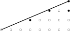
Figure 1. Generators in the $(\deg z,-ord_{P_{2}}(z))$ lattice

Also note that $e_{j}^{\prime}+2k=7+2k\nmid 2=e_{i}-e_{j}^{\prime}$ for all $i,j\in J=\{2,3\}$ such that $j\neq i$ and for all $k\geq 0$. Thus, $s_{\sigma,J}(i,k)=\emptyset$ for each $i\in J$. Furthermore, $\deg\lfloor e_{i}L\rfloor=\deg\lfloor 9L\rfloor=2\lfloor\frac{4\cdot 9}{9}\rfloor+\lfloor\frac{9}{3}\rfloor-9=2$, so LABEL:custom:Ad-iii is satisfied and $(\sigma,\mathscr{X}^{\prime},\{2,3\})$ is admissible.

Example 4.11.

Let $(\mathscr{X}^{\prime},0,L^{\prime})$ be a log spin curve of genus $1$ with $L^{\prime}=P-Q+\frac{1}{3}P_{1}+\frac{1}{3}P_{2}$, as in Example  3.5. Here, we check that $(\mathscr{X}^{\prime},L^{\prime},\{1,2\})$ is admissible.

Recall that

$$R_{L^{\prime}}\cong{\Bbbk}[u,x_{3},y_{3},y_{4}]/(x_{3}y_{3}-\alpha uy_{4},y_{4}^{2}-\beta x_{3}^{2}u-\gamma y_{3}^{2}u).$$

We have two generators $x_{3}$ and $y_{3}$ in degree 3 with a pole of order $1=\frac{3-1}{2}$ by construction. Hence, LABEL:custom:Ad-i holds. We next check LABEL:custom:Ad-ii for the point $P_{1}$, as the case of $P_{2}$ is symmetric. Here, by construction

$$\frac{-\operatorname{ord}_{P_{1}}(z)}{\operatorname{ord}(z)}=\begin{cases}0&\text{ if }z\in\{u,y_{3}\}\\ \frac{1}{4}&\text{ if }z=y_{4}.\end{cases}$$

Since $0,\frac{1}{4}<\frac{1}{3}$, LABEL:custom:Ad-ii holds. Finally, to check LABEL:custom:Ad-iii, note that $\max_{k\geq 0}S_{\sigma,J}(i,k)=0.$ Therefore, $\deg\lfloor 5L\rfloor=2>1=(2g-1)+0$.

The following lemma will slightly strengthen condition LABEL:custom:Ad-ii from Definition  4.9. This improvement is crucial in the proof of part (c) of Lemma  4.15.

Lemma 4.12.

For any $z$ as in condition LABEL:custom:Ad-ii of definition  4.9 the inequality LABEL:custom:Ad-ii implies the tighter inequality that

$$-\operatorname{ord}_{Q_{i}}^{L_{X}^{\prime}}(z)\leq\deg(z)\frac{{e_{i}^{\prime}}-1}{2{e_{i}^{\prime}}}-\frac{1}{e_{i}^{\prime}}$$

Proof.

We know by LABEL:custom:Ad-ii that

$$-\operatorname{ord}_{Q_{i}}^{L_{X}^{\prime}}(z)<\deg(z)\frac{{e_{i}^{\prime}}-1}{2{e_{i}^{\prime}}}$$

If we write $\frac{\alpha}{\beta}=\deg(z)\frac{e_{i}^{\prime}-1}{2e_{i}^{\prime}}$ as a fraction in lowest terms, then we see $\beta\mid e_{i}^{\prime}$ since $e_{i}^{\prime}-1$ is even. Therefore, since $-\operatorname{ord}_{Q_{i}}^{L_{X}^{\prime}}(z)$ is an integer, we must have

$$-\operatorname{ord}_{Q_{i}}^{L_{X}^{\prime}}(z)\leq\deg(z)\frac{{e_{i}^{\prime}}-1}{2{e_{i}^{\prime}}}-\frac{1}{\beta}\leq\deg(z)\frac{{e_{i}^{\prime}}-1}{2{e_{i}^{\prime}}}-\frac{1}{e_{i}^{\prime}}.$$

∎

Lemma 4.13.

If $(\mathscr{X}^{\prime},\Delta,L^{\prime})$ is a log spin curve, $(\mathscr{X}^{\prime},L^{\prime},J)$ is admissible and $W\subseteq J$ is any subset, then $(\mathscr{X}^{\prime},L^{\prime},W)$ is also admissible.

Proof.

Each of the conditions LABEL:custom:Ad-i, LABEL:custom:Ad-ii, and LABEL:custom:Ad-iii hold for $W$ if they hold for $J$. ∎

Remark 4.14.

For our inductive arguments in Theorems  5.6,  6.1, and  7.4, we will often add in a single stacky point with stabilizer order $3$. Say $(\mathscr{X},\Delta,L)$ is a log spin curve with signature $\sigma:=(g;e_{1},\ldots,e_{r};\delta)=(g;3,\ldots,3;\delta)$, and our base cases include signatures $\sigma$ characterized by one of the following: cases, which we will soon refer to in Lemma  4.15:

1. $g=0,e_{1}=\cdots=e_{r}=3,\delta=0$, and $r\geq 5$

2. $g=1,e_{1}=\cdots=e_{r}=3,\delta=0$, and $r\geq 2$

3. $g\geq 2,e_{1}=\cdots=e_{r}=3,\delta$ arbitrary, and $r\geq 1$.

Lemma 4.15.

Suppose $(\mathscr{X}^{\prime},\Delta,L^{\prime})$ is a log spin curve with coarse space $X^{\prime}$ and signature $\sigma:=(g;e_{1}^{\prime},\ldots,e_{r}^{\prime};\delta)$. Define $R^{\prime}:=R_{L^{\prime}}$. Further, assume either

1. $(\mathscr{X}^{\prime},L^{\prime},J)$ is admissible with generators $x_{1},\ldots,x_{m}\in R^{\prime}$ and $y_{i,e_{i}^{\prime}}\in R^{\prime}$ for all $i\in J$, as in Definition  4.9 or

2. $\sigma$ is one of the signatures described in Cases LABEL:custom:three-cases-1, LABEL:custom:three-cases-2 and LABEL:custom:three-cases-3 of Remark  4.14 and $y_{1,3}=y_{2,3}=\ldots=y_{r,3}$ is a rational section of ${\mathscr{O}}(L_{X})$ with $\operatorname{ord}_{P_{i}}^{L_{X}^{\prime}}(y_{1,3})=1$ for $1\leq i\leq r$.

Let $(\mathscr{X},\Delta,L)$ be another log spin curve with coarse space $X$, so that $X\cong X^{\prime}$ and with signature $(g;e_{1},\ldots,e_{r};\delta)$ such that $e_{i}=e_{i}^{\prime}+2$ for all $i\in J$ and $e_{j}=e_{j}^{\prime}$ for $j\notin J$. Define $R:=R_{L}$. Then the following are true:

1. For all $i\in J$, there exists $y_{i,e_{i}}\in H^{0}(\mathscr{X},e_{i}(K_{\mathscr{X}}))$ so that

   $$-\operatorname{ord}_{Q_{i}}^{L_{X}^{\prime}}(y_{i,e_{i}})=\frac{e_{i}-1}{2}$$

   and

   $$\frac{-\operatorname{ord}_{Q_{j}}^{L_{X}^{\prime}}(y_{i,e_{i}})}{\deg(y_{i,e_{i}})}\leq\frac{{e_{j}^{\prime}}-1}{2{e_{j}^{\prime}}}-\frac{1}{\deg(y_{i,e_{i}})e_{j}^{\prime}}$$

   for all $j\in J$ with $j\neq i$.

2. A choice of elements $y_{1,e_{1}},\ldots,y_{r,e_{r}}$ as in part (a) minimally generate $R$ over $R^{\prime}$.

3. Endow ${\Bbbk}[y_{i,e_{i}}]_{i\in J}$ and ${\Bbbk}[x_{1},\ldots,x_{m},y_{i,e_{i}^{\prime}}]_{i\in J}$ with graded monomial orders and give ${\Bbbk}[y_{i,e_{i}}]_{i\in J}\otimes{\Bbbk}[x_{1},\ldots,x_{m},y_{i,e_{i}^{\prime}}]_{i\in J}$ block order. Let $I$ be the kernel of ${\Bbbk}[x_{1},\ldots,x_{m},y_{i,e_{i}^{\prime}},y_{i,e_{i}}]_{i\in J}\to R$. Then,

   $$\operatorname{in_{\prec}}(I)\; =\;\operatorname{in_{\prec}}(I^{\prime}){\Bbbk}[x,y]$$

   $$+\;\langle y_{j,e_{j}}x_{i}:1\leq i\leq m,j\in J\rangle$$

   $$+\;\langle y_{j,e_{j}}y_{i,e_{i}^{\prime}}:i,j\in J,i\neq j\rangle$$

   $$+\;\langle y_{j,e_{j}}y_{i,e_{i}}:i,j\in J,i\neq j\rangle.$$

4. The triple $(\mathscr{X},L^{\prime},J)$ is admissible.

Idea of Proof:

The construction of the $y_{i,e_{i}}$ in Part (a) uses Riemann–Roch and condition  LABEL:custom:Ad-iii. The inequality in Part (a) follows from the fact that $L$ is similar to $L^{\prime}$, but with some of the $e_{i}$ incremented by $2$. Part (b) follows because the sub-lattice spanned by $y_{i,e_{i}}$ and $y_{i,e_{i}^{\prime}}$ has determinant $1$ for $i\in J$, so the generators in Part (a) generate all of $R_{L}$ over $R_{L^{\prime}}$. To check part (c), we construct relations between the generators of $R_{L}$ over $R_{L^{\prime}}$: we note that an element lies in $R_{L^{\prime}}$ if and only if its pole order at $P_{i}$ for $i\in J$ is not too large, and use Lemma  4.12 to bound pole orders. Part (d) follows fairly easily from the definition of admissibility.

Proof.

We prove this in case (1). Case (2) follows a similar procedure.

Part (a): By Definition  4.9, for all $i\in J$

$$S(i,0)=\{j\in J:j\neq i\text{ and }e_{j}^{\prime}\mid e_{i}-e_{j}^{\prime}\}=\{j\in J:j\neq i\text{ and }e_{j}^{\prime}\mid e_{i}\}.$$

Define

$$E_{i}=\sum_{j\in S(i,0)}Q_{j}.$$

The assumption LABEL:custom:Ad-iii implies

$$\deg\left(e_{i}L^{\prime}-E_{i}\right)\geq\max(2g-1,0),$$

and so $H^{0}(\mathscr{X}^{\prime},e_{i}L^{\prime}-E_{i}+Q_{i})$ is base point free by Riemann–Roch. Hence, a general element

$$y_{i,e_{i}}\in H^{0}(\mathscr{X}^{\prime},e_{i}L^{\prime}-E_{i}+Q_{i})$$

satisfies

$$-\operatorname{ord}_{Q_{i}}^{L_{X}^{\prime}}(y_{i,e_{i}})=\left\lfloor e_{i}\frac{{e_{i}^{\prime}}-1}{2{e_{i}^{\prime}}}\right\rfloor+1=\frac{e_{i}-1}{2}.$$

Noting that

$$\lfloor e_{i}L^{\prime}\rfloor+Q_{i}\leq\lfloor e_{i}L\rfloor,$$

we obtain an inclusion

$$H^{0}(\mathscr{X}^{\prime},e_{i}L^{\prime}-E_{i}+Q_{i})\rightarrow H^{0}(\mathscr{X},e_{i}L-E_{i})\subseteq H^{0}(\mathscr{X},e_{i}L)$$

meaning that $y_{i,e_{i}}\in H^{0}(\mathscr{X},e_{i}L)$ satisfies the first part of claim (a).

We next show $y_{i,e_{i}}$ also satisfies the second part of the claim of $(a),$ by considering separately the cases in which $j\in S(i,0),$ and $j\notin S(i,0)$.

If $j\in S(i,0)$, then $E_{i}\geq Q_{j}$ gives $y_{i,e_{i}}\in H^{0}(\mathscr{X}^{\prime},e_{i}L^{\prime}-E_{i}+Q_{i})$ an extra vanishing condition at $Q_{j}$, so

$$-\operatorname{ord}_{Q_{j}}^{L_{X}^{\prime}}(y_{i,e_{i}})\leq e_{i}\frac{{e_{j}^{\prime}}-1}{2{e_{j}^{\prime}}}-1\leq e_{i}\frac{{e_{j}^{\prime}}-1}{2{e_{j}^{\prime}}}-\frac{1}{e_{j}^{\prime}}.$$

If instead $j\neq i$ and $j\notin S(i,0)$, then since $e_{j}^{\prime}\nmid e_{i}$, we know $e_{i}\frac{{e_{j}^{\prime}}-1}{2{e_{j}^{\prime}}}\notin{\mathbb{Z}}$, so

$$-\operatorname{ord}_{Q_{j}}^{L_{X}^{\prime}}(y_{i,e_{i}})\leq\left\lfloor e_{i}\frac{{e_{j}^{\prime}}-1}{2{e_{j}^{\prime}}}\right\rfloor\leq e_{i}\frac{{e_{j}^{\prime}}-1}{2{e_{j}^{\prime}}}-\frac{1}{e_{j}^{\prime}},$$

completing the proof of (a).

Part (b): Define $R_{0}=R^{\prime}$ and for $i\in\{1,\ldots,r\},$ inductively define

$$R_{i}=\begin{cases}R_{i-1}&\text{ if }i\notin J\\ R_{i-1}[y_{i,e_{i}}]&\text{ if }i\in J.\end{cases}$$

To prove (b), it suffices to show that elements of the form $y_{i,e_{i}^{\prime}}^{a}y_{i,e_{i}}^{b}$ with $a\geq 0,b>0$ form a ${\Bbbk}$-basis for $R_{i}$ over $R_{i-1}$. These elements do not lie in $R_{i-1}$ because the pole order of $y_{i,e_{i}^{\prime}}^{a}y_{i,e_{i}}^{b}$ at $Q_{i}$ is larger than that of any element in the $k^{th}$ component of $R_{i-1}$. Additionally, these elements are linearly independent amongst themselves because of injectivity of the linear map

$$(a,b)\mapsto\left(\deg\left(y_{i,e_{i}^{\prime}}^{a}y_{i,e_{i}}^{b}\right),-\operatorname{ord}_{Q_{i}}^{L_{X}^{\prime}}\left(y_{i,e_{i}^{\prime}}^{a}y_{i,e_{i}}^{b}\right)\right)=(a,b)\begin{pmatrix}e_{i}-2&\frac{e_{i}-3}{2}\\ e_{i}&\frac{e_{i}-1}{2}\end{pmatrix}.$$

Furthermore, $\{y_{i,e_{i}^{\prime}}^{a}y_{i,e_{i}}^{b}:a\geq 0,b>0\}$ span $R_{i}$ over $R_{i-1}$, because the set of integer lattice points in the cone generated by the vectors $\left(e_{i}-2,\frac{e_{i}-3}{2}\right)$ and $\left(e_{i},\frac{e_{i}-1}{2}\right)$ is saturated, because the corresponding determinant is

$$(e_{i}-2)\frac{e_{i}-1}{2}-e_{i}\frac{e_{i}-3}{2}=1.$$

This completes part (b).

Part (c): To show (c), we wish to show that $y_{i,e_{i}}z\in R^{\prime}$ for all generators $z$ of $R^{\prime}$ with $z\neq y_{i,e_{i}}\text{ and }z\neq y_{i,e_{i}^{\prime}}$. By definition of $H^{0}(\mathscr{X},L^{\prime})$, note that $f\in R$ further satisfies $f\in R^{\prime}$ if and only if for all $j\in J$ we have

(4.4) $$-\operatorname{ord}_{Q_{j}}^{L_{X}^{\prime}}(f)\leq\deg(f)\left(\frac{{e_{j}^{\prime}}-1}{2{e_{j}^{\prime}}}\right).$$

Now fix $i\in J$. We check that Inequality  (4.4) holds with $f=y_{i,e_{i}}z$, implying $y_{i,e_{i}}z\in R^{\prime}$ in the three following cases:

Case 1: $j\notin\{i\}\cup S(i,0).$

Here, $L|_{Q_{j}}=L^{\prime}|_{Q_{j}},$ so

$$-\operatorname{ord}_{Q_{j}}^{L_{X}^{\prime}}(y_{i,e_{i}})-\operatorname{ord}_{Q_{j}}^{L_{X}^{\prime}}(z)\leq e_{i}\frac{{e_{j}^{\prime}}-1}{2{e_{j}^{\prime}}}+\deg(z)\frac{{e_{j}^{\prime}}-1}{2{e_{j}^{\prime}}}=\deg(y_{i,e_{i}}z)\frac{{e_{j}^{\prime}}-1}{2{e_{j}^{\prime}}}.$$

Case 2: $j=i.$

By part (a), condition LABEL:custom:Ad-ii, and Lemma  4.12 we have

$$-\operatorname{ord}_{Q_{j}}^{L_{X}^{\prime}}(y_{i,e_{i}})-\operatorname{ord}_{Q_{j}}^{L_{X}^{\prime}}(z) \leq\frac{e_{j}-1}{2}+\deg(z)\left(\frac{{e_{j}^{\prime}}-1}{2{e_{j}^{\prime}}}\right)-\frac{1}{e_{j}^{\prime}}$$

$$=\frac{e_{j}-1}{2}-\frac{1}{e_{j}^{\prime}}+\deg(z)\left(\frac{{e_{j}^{\prime}}-1}{2{e_{j}^{\prime}}}\right)$$

$$=\frac{e_{j}(e_{j}-3)}{2(e_{j}-2)}+\deg(z)\left(\frac{{e_{j}^{\prime}}-1}{2{e_{j}^{\prime}}}\right)$$

$$=\deg(y_{i,e_{i}}z)\frac{{e_{j}^{\prime}}-1}{2{e_{j}^{\prime}}}.$$

Case 3: $j\in S(i,0).$

In this case, we may first assume $z\neq y_{j,e_{j}}$, as this is covered by case 2, with $i$ and $j$ reversed. Hence,

$$-\operatorname{ord}_{Q_{j}}^{L_{X}^{\prime}}(z)\leq\deg z\frac{{e_{j}^{\prime}}-1}{2{e_{j}^{\prime}}},$$

implying

$$-\operatorname{ord}_{Q_{j}}^{L_{X}^{\prime}}(y_{i,e_{i}})-\operatorname{ord}_{Q_{j}}^{L_{X}^{\prime}}(z) \leq e_{i}\frac{{e_{j}^{\prime}}-1}{2{e_{j}^{\prime}}}+\deg z\frac{{e_{j}^{\prime}}-1}{2{e_{j}^{\prime}}}=\deg(y_{i,e_{i}}z)\frac{{e_{j}^{\prime}}-1}{2{e_{j}^{\prime}}},$$

completing part (c).

Part (d): To check (d), we show LABEL:custom:Ad-i, LABEL:custom:Ad-ii, and LABEL:custom:Ad-iii are satisfied. We know LABEL:custom:Ad-i holds by part (b), taking the $y_{i,e_{i}}$ as the generators in degree $e_{i}$. Next, LABEL:custom:Ad-ii is strictly monotonic in the $e_{i}$ and hence also holds for $(\mathscr{X},J)$. Finally, if LABEL:custom:Ad-iii holds for $e$ then it holds for $e+2$ by definition. This is where we use that LABEL:custom:Ad-iii holds for $k>0$ and not just for $k=0$. ∎

Corollary 4.16.

Suppose $(\mathscr{X}^{\prime},L^{\prime},J^{\prime})$ is admissible with signature $\sigma^{\prime}=(e_{1}^{\prime},\ldots,e_{r}^{\prime})$ or $\sigma$ satisfies one of the conditions of Remark  4.14. Let $J^{\prime}=\{t,t+1,\ldots,r\}$ and $e_{1}^{\prime}\leq e_{2}^{\prime}\leq\cdots\leq e_{t}^{\prime}=e_{t+1}^{\prime}=\cdots=e_{r}^{\prime}$, so that $(\mathscr{X}^{\prime},\Delta,L)$ satisfies the conditions of Lemma  4.15 and Theorem  1.1. Then, for any spin curve $(\mathscr{X},\Delta,L)$ so that $\mathscr{X}$ and $\mathscr{X}^{\prime}$ have the same coarse space $X=X^{\prime}$ with the same set of stacky points, and $\mathscr{X}$ has signature $(g;e_{1},\ldots,e_{r};\delta)$ with $e_{1}\leq e_{2}\leq\cdots e_{r}$ so that

$$e_{i}=e_{i}^{\prime} \text{ if }i\notin J$$

$$e_{i}\geq e_{i}^{\prime} \text{ if }i\in J$$

then Theorem  1.1 holds for $(\mathscr{X},\Delta,L)$.

Proof.

For $t\leq i\leq r$, let $(\mathscr{X}_{i},\Delta,L_{i})$ be the log spin curve with coarse space $X_{i}$ so that $X_{i}=X^{\prime},$ with the same stacky points as $(\mathscr{X}^{\prime},\Delta,L),$ and having signature $(g;e_{1},\ldots.e_{i-1},e_{i},e_{i},\ldots,e_{i};\delta).$ Let $J_{i}=\{i,\ldots,r\}.$ Note that $(\mathscr{X}_{0},L_{0},J_{0})=(\mathscr{X}^{\prime},L^{\prime},J^{\prime})$ and $(\mathscr{X}_{r},L_{r},J_{r})=(\mathscr{X},L,\{r\})$.

Let $(*_{i})$ denote the condition that $(\mathscr{X}_{i},\Delta,L_{i})$ satisfies the conditions of Lemma  4.15 and Theorem  1.1, and $(\mathscr{X}_{i},L_{i},J_{i})$ is admissible. Since $(*_{0})$ holds by assumption, it suffices to show that if $(*_{i})$ holds then so does $(*_{i+1})$. Indeed, $(\mathscr{X}_{i},L_{i},J_{i+1})$ is admissible by an application of Lemma  4.13 and the fact that $J_{i+1}\subseteq J_{i}$. Then, applying Lemma  4.15 with the fixed set $J_{i+1}$ repeatedly ($\frac{e_{i+1}-e_{i}}{2}$ many times) yields $(*_{i+1})$. ∎

5. Genus At Least Two

We now consider the case when the genus is at least 2. In this case, we are able to bound the degrees of generators of $R_{L}$ and its ideal of relations. In this section, we do not obtain explicit presentations of $R_{L}$. This contrasts with Sections  6 and  7 where we not only obtain bounds, but also obtain inductive presentations. The tradeoff is that in the genus zero and genus one cases, we have to deal with explicit base cases. In this section we apply general results.

5.1. Bounds on Generators and Relations in Genus At Least Two

The main result of this subsection is that for a log spin curve with no stacky points $(X,\Delta,L)$, the spin canonical ring $R_{L}$ is generated in degree at most $5$, with relations in degree at most $10$. The case that $\Delta=0$ was completed by Reid [Rei90, Theorem 3.4]. For $\Delta>0$, the generation bound is shown in Lemma  5.1 and the relations bound is shown in Lemma  5.4. Throughout this subsection, we will implicitly use Remark  2.12, which implies $\deg 2L\geq 2g$ so $H^{0}(X,2L)$ is basepoint-free by Riemann–Roch. We summarize the results of this subsection in Corollary  5.5.

The proofs of this subsection results are similar to those in Neves  [Nev03, Proposition III.4 and Proposition III.12]. However, the statements differ, as we assume $\Delta>0$ instead of $\Delta=0$ and do not assume there is a basepoint-free pencil contained in $H^{0}(X,L).$

Lemma 5.1.

Let $(X,\Delta,L)$ be a log spin curve of signature $(g;-;\delta),$ (where $-$ means $X$ is a bona fide scheme and has no stacky points,) with $g\geq 2$ and $\Delta>0.$ Let $s_{1}$, $s_{2}\in H^{0}(X,2L)$ be two independent sections such that the vector subspace $V=\operatorname{span}(s_{1},s_{2})\subseteq H^{0}(K)$ is basepoint-free. Then, the map

$$V\otimes H^{0}(nL)\rightarrow H^{0}((n+2)L)$$

is surjective if $n\geq 4$. In particular, $R_{L}$ is generated in degree at most $5.$

Proof.

To show there are no new generators in degree at least $6$, it suffices to show that if $n\geq 4$, the map

$$H^{0}(nL)\otimes H^{0}(2L)\rightarrow H^{0}((n+2)L)$$

is surjective. Indeed, since $V=\operatorname{span}(s_{1},s_{2})\subseteq H^{0}(K)$ is basepoint-free, by the basepoint-free pencil trick (see [SD73, Lemma 2.6] for a proof), we obtain an exact sequence

$$0\longrightarrow H^{0}((n-2)L)\longrightarrow V\otimes H^{0}(nL)\overset{f}{\longrightarrow}H^{0}((n+2)L)$$

We wish to show $f$ is surjective. Note that $\dim_{\Bbbk}\ker f=\dim_{\Bbbk}H^{0}((n-2)L)=(n-3)(g-1+\frac{\delta}{2})$ using Riemann–Roch and the assumption $n\geq 4.$ Additionally, $\dim_{\Bbbk}V\otimes H^{0}(nL)=2\cdot(n-1)(g-1+\frac{\delta}{2})$, again using Riemann–Roch. Therefore,

$$\dim_{\Bbbk}\text{im }f =2\cdot(n-1)(g-1+\frac{\delta}{2})-(n-3)(g-1+\frac{\delta}{2})$$

$$=(n+1)(g-1+\frac{\delta}{2})=\dim_{\Bbbk}H^{0}((n+2)L).$$

Ergo, $f$ is surjective. ∎

The next step is to bound the degrees of the relations of $R_{L}$ when $\Delta>0$. This is done in Proposition  5.4 by using the basepoint-free pencil trick to show that if a relation lies in a sufficiently high degree, it lies in the ideal generated by the relations in lower degrees. In Definition  5.2, we fix notation for the ideal generated by lower degrees relations:

Definition 5.2.

Let $(X,\Delta,L)$ be a log spin curve of signature $(g;-;\delta)$ with $g\geq 2$ and $\Delta>0.$ Choose generators $x_{1},\ldots,x_{n}$ of $R_{L}$ so that we obtain a surjection $\phi:{\Bbbk}[x_{1},\ldots,x_{n}]\twoheadrightarrow R_{L}$ with kernel $I_{L}$. Let $I_{L,k}$ be the $k^{\text{th}}$ graded piece of $I_{L}$ and define

$$J_{L,k}=\sum_{j=1}^{k-1}{\Bbbk}[x_{1},\ldots,x_{n}]_{j}\cdot I_{L,k-j}.$$

Lemma 5.3.

Let $(X,\Delta,L)$ be a log spin curve of genus $g\geq 2,$ so that $\Delta>0.$ Choose generators $x_{1},\ldots,x_{n}$ of $R_{L}$ so that we obtain a surjection $\phi:{\Bbbk}[x_{1},\ldots,x_{n}]\twoheadrightarrow R_{L}$ with kernel $I_{L}$. Let $s_{1},s_{2}\in{\Bbbk}[x_{1},\ldots,x_{n}]_{2}$ be two elements so that $\>\operatorname{span}(\phi(s_{1}),\phi(s_{2}))$ $=V\subseteq H^{0}(X,2L)$ is basepoint-free. For any $f\in{\Bbbk}[x_{1},\ldots,x_{n}]$ such that $\deg f\geq 11,$ there exist $g,h\in{\Bbbk}[x_{1},\ldots,x_{n}]_{k-2}$ so that $s_{1}g+s_{2}h\equiv f\bmod J_{L,k}.$

Proof.

By Lemma  5.1, $\deg x_{i}\leq 5$ for $1\leq i\leq n$. Therefore, we may write $f=\sum_{i=1}^{n}a_{i}x_{i}$ with $a_{i}\in{\Bbbk}[x_{1},\ldots,x_{n}]_{k-\deg x_{i}}$. We next show that for all $1\leq i\leq n$ there exist $g_{i},h_{i}\in{\Bbbk}[x_{1},\ldots,x_{n}]_{k-\deg x_{i}-2}$ so that $a_{i}=s_{1}g_{i}+s_{2}h_{i}\bmod I_{L,\deg a_{i}}.$

By Lemma  5.1,

$$V\otimes H^{0}((\deg f-\deg x_{i}-2)L)\rightarrow H^{0}((\deg f-\deg x_{i})L)$$

is surjective because $\deg f\geq 11$ implies that

$$\deg a_{i}=\deg f-\deg x_{i}-2\geq 4.$$

In particular, there exist $\alpha_{i},\beta_{i}\in R_{L}$ so that

$$\phi(a_{i})=\phi(s_{1})\cdot\alpha_{i}+\phi(s_{2})\cdot\beta_{i}.$$

Choosing $g_{i},h_{i}\in{\Bbbk}[x_{1},\ldots,x_{n}]_{\deg(a_{i})-2}$ for $1\leq i\leq n$ so that $\phi(g_{i})=\alpha_{i},\phi(h_{i})=\beta_{i}$, we have

$$a_{i}\equiv s_{1}g_{i}+s_{2}h_{i}\bmod I_{L,\deg a_{i}},$$

as claimed.

Finally, we may then take $g=\sum_{i}g_{i}x_{i},\>h=\sum_{i}h_{i}x_{i},$ so that

$$f \equiv\sum_{i}a_{i}x_{i}\equiv\sum_{i}(s_{1}g_{i}+s_{2}h_{i})x_{i}\equiv s_{1}\left(\sum_{i}g_{i}x_{i}\right)+s_{2}\left(\sum_{i}h_{i}x_{i}\right)$$

$$\equiv s_{1}g+s_{2}h\bmod J_{L,k}.$$

∎

Proposition 5.4.

Let $(X,\Delta,L)$ be a log spin curve of signature $(g;-;\delta)$ with $g\geq 2$ and $\Delta>0.$ Then $I_{L}$ is generated in degree at most $10$.

Proof.

Suppose $f\in I_{L}$ with $\deg f\geq 11$. To complete the proof, it suffices to show $f\in J_{L,k}$. By Lemma  5.3, this is the same as checking $s_{1}g+s_{2}h\in J_{L,k}$ where $\phi(s_{1}),\phi(s_{2})\in H^{0}(X,2L)$ are two sections so that $\operatorname{span}(\phi(s_{1}),\phi(s_{2}))=V\subseteq H^{0}(K)$ is basepoint-free. Consider the map

we know that $\phi(s_{1})\phi(g)+\phi(s_{2})\phi(h)\mapsto 0$. So by the explicit isomorphism given in the proof of the basepoint-free pencil trick, as shown in the proof of [SD73, Lemma 2.6], there exists some $\rho\in{\Bbbk}[x_{1},\ldots,x_{n}]$ so that $\phi(\rho)\in H^{0}((\deg f-4)L)$ satisfies $\phi(g)=\phi(s_{2})\phi(\rho)$ and $\phi(h)=-\phi(s_{1})\phi(\rho)$. Therefore, $g\equiv s_{2}\rho\bmod I_{L,k-2}$ and $h\equiv-s_{1}\rho\bmod I_{L,k-2}$. Hence,

$$s_{1}g+s_{2}h\equiv s_{1}(s_{2}\rho)+s_{2}(-s_{1}\rho)\equiv 0\bmod J_{L,k}.$$

∎

We now summarize what we have shown.

Corollary 5.5.

Let $(X,\Delta,L)$ be a log spin curve of signature $(g;-;\delta)$ with $g\geq 2$. Then $X$ has minimal generators in degree at most $5$ and minimal relations in degree at most $10$.

Proof.

If $\delta=0$, the result is immediate from Reid [Rei90, Theorem 3.4]. Otherwise, if $\delta>0$, the bound on the degrees of minimal generators follows from Lemma  5.1, while the bound on the degrees of minimal relations follows from Proposition  5.4. ∎

5.2. Main Theorem for Genus At Least Two

We are ready to prove our main theorem, Theorem  1.1 in the case $g\geq 2$. The idea of the proof is to use Corollary 5.5 to complete the base case when $L=L_{X}$ and then apply Lemma  4.4, Lemma  4.7, and Lemma  4.15 to complete the induction step.

Theorem 5.6.

Let $g\geq 2$ and let $(\mathscr{X},\Delta,L)$ be a log spin curve with signature $(g;e_{1},\ldots,e_{r};\delta)$. Then the log spin canonical ring $R(\mathscr{X},\Delta,L)$ is generated as a ${\Bbbk}$-algebra by elements in degree at most $e=\max(5,e_{1},\ldots,e_{r})$ with minimal relations in degree at most $2e$.

Proof.

As the base case, let $L=L_{X}\in\operatorname{Div}X$ satisfy $2L\sim 2K_{X}+\Delta$. By Corollary  5.5, the theorem holds for $(\mathscr{X},\Delta,L_{X})$.

Next, suppose the theorem holds for $L^{\prime}=L_{X}+\sum_{i=1}^{r-1}\frac{1}{3}P_{i}$. Let $L$ be a log spin canonical divisor of the form $L=L_{X}+\sum_{i=1}^{r}\frac{1}{3}P_{i}$, which means that $L=L^{\prime}+\frac{1}{3}P_{r}$. If $P_{r}$ is a basepoint of $L^{\prime}$, then the theorem holds for $L$ by Lemma  4.7. Otherwise, $P_{r}$ is not a basepoint of $L^{\prime}$, meaning that in particular $R_{L^{\prime}}$ is saturated in 1. Therefore, since $P_{r}$ is a not basepoint of $L^{\prime}$, Equation  4.1 holds by Riemann–Roch. In this case, the theorem holds for $L$ by Lemma  4.4.

We have thus shown the theorem for all $(\mathscr{X},\Delta,L)$ with $g\geq 2$ and signature $(g;3,\ldots,3;\delta)$. Therefore, by Corollary  4.16, this theorem holds for all log spin curves $(\mathscr{X},\Delta,L)$. ∎

Remark 5.7.

For this remark, we retain the terminology from the proof of Theorem  5.6. Suppose $e:=\max(e_{1},\ldots,e_{r}).$ Then, $R_{L}$ has a generator in degree $e$ when $e\geq 5$ and a relation in degree at least $2e-4$ when $e\geq 7$. Since the proof of Theorem  6.1 is given by inductively applying Lemmas  4.4 and  4.7, we obtain that $R_{L}$ is minimally generated over $R_{L^{\prime}}$ by an element in degree $e,$ assuming $e\geq 5$. Furthermore, if $e\geq 7$ and $e_{i}=e,$ then there must be a relation with leading term $y_{i,e_{i}}\cdot y_{i,e_{i}-4}.$ Hence, there is a relation in degree at least $2e-4$. Further, by examining the statements of Lemma  4.4 and 4.7 in the case that there are $1\leq i<j\leq r$ with $e_{i}=e_{j}=e$, then, there is necessarily a relation with leading term $y_{i,e_{i}}\cdot y_{j,e_{j}}$ in degree $2e$. This analysis also applies to the cases that $g=0$ and $g=1$.

6. Genus One

In this section, we prove Theorem  1.1 in the case that $g=1$. We follow a similar inductive strategy as in the genus $g\geq 2$ case, except unlike in the $g\geq 2$ case we obtain explicit generators and relations here.

In the case of a genus 1 curve, $X$ with no stacky points, we know $K_{X}\sim 0$, and therefore the only possibilities for log spin canonical divisors are $L^{\prime}\sim 0$ or $L^{\prime}\sim P-Q$ where $P,Q$ are distinct points, fixed under the hyperelliptic involution. We inductively construct presentations by adding points through Lemmas  4.4 and  4.7 and incrementing the values of the $e_{i}$’s using Lemma  4.15.

6.1. Genus One Base Cases

In this subsection we set up the base cases needed for our inductive approach, of proving Theorem  1.1 in the case $g=1$.

$L^{\prime}$	Generator Degrees	Degrees of Minimal Relations	$e$
$0$	$\{1\}$	$\emptyset$	$1$
$\frac{3}{7}P_{1}$	$\{1,5,7\}$	$\{15\}$	$7$
$\frac{1}{3}P_{1}+\frac{1}{3}P_{2}$	$\{1,3,3\}$	$\{6\}$	$5$
$P-Q+\frac{2}{5}P_{1}$	$\{2,3,5\}$	$\{12\}$	$5$
$P-Q+\frac{1}{3}P_{1}+\frac{1}{3}P_{2}$	$\{2,3,3,4\}$	$\{6,8\}$	$5$

Table 1. Genus 1 Base Cases

Generators and relations for $R_{L^{\prime}}$ with $L^{\prime}=0,\>L^{\prime}=P-Q+\frac{1}{3}P_{1}+\frac{1}{3}P_{2},$ and $L^{\prime}=P-Q+\frac{2}{5}P_{1}$ were checked in Examples  3.1, 3.5, and 3.6 respectively. Note that admissibility for $(\mathscr{X}^{\prime},0,P-Q+\frac{1}{3}P_{1}+\frac{1}{3}P_{2})$ is verified in Example  4.11. The verification of admissibility for the other cases is similar.

The base cases of $L^{\prime}=\frac{3}{7}P_{1}$ and $L^{\prime}=\frac{1}{3}P_{1}+\frac{1}{3}P_{2}$ can be similarly computed. Although $L^{\prime}=P-Q+\frac{2}{5}P_{1},$ and $L^{\prime}=\frac{3}{7}P_{1}$ are used as base cases for the induction, they are also exceptional cases; see Table  2.

6.2. Genus One Exceptional Cases

Let $\mathscr{X}$ be a stacky curve, with $P,Q$ distinct hyperelliptic fixed points on $X$. The following table provides a list of all cases which are not generated in degrees $e:=\max(5,e_{1},\ldots,e_{r})$ with relations in degrees $2e$, as described in Theorem  6.1.

$L^{\prime}$	Generator Degrees	Degrees of Minimal Relations	$e$
$P-Q$	$\{2\}$	$\emptyset$	$1$
$P-Q+\frac{1}{3}P_{1}$	$\{2,3,7\}$	$\{14\}$	$5$
$P-Q+\frac{2}{5}P_{1}$	$\{2,3,5\}$	$\{12\}$	$5$
$\frac{1}{3}P_{1}$	$\{1,6,9\}$	$\{18\}$	$5$
$\frac{2}{5}P_{1}$	$\{1,5,8\}$	$\{16\}$	$5$
$\frac{3}{7}P_{1}$	$\{1,5,7\}$	$\{15\}$	$7$

Table 2. Genus 1 Exceptional Cases

We have already checked the case of $L^{\prime}=P-Q+\frac{1}{5}P_{1}$ above in Example  3.6. The other cases are similar.

6.3. Main Theorem for Genus One

We now have all the tools necessary to prove our main theorem,  1.1 in the case $g=1$.

Theorem 6.1.

Let $(\mathscr{X},\Delta,L)$ log spin curve with signature $\sigma:=(1;e_{1},\ldots,e_{r};\delta)$. If $g=1$, then the log spin canonical ring $R(\mathscr{X},\Delta,L)$ is generated as a ${\Bbbk}$-algebra by elements of degree at most $\max(5,e_{1},\ldots,e_{r})$ and has relations in degree at most $2e,$ so long as $\sigma$ does not lie in a finite list of exceptional cases, as listed in Table  2.

Idea of Proof:

We check the theorem in two cases, depending on if $\delta>0$. If $\delta>0$, we first check that the theorem holds for $L_{X}$ by inductively adding in log points to the base case of $L_{X}^{\prime}=0$. Then we check that the theorem holds for $L$ by adding stacky points and then inductively raising the stabilizer orders of stacky points in the following sequence of steps. When raising the stacky orders, it is important that we increment the stabilizer orders of as many stacky points as possible to maintain admissibility for the maximal possible sets of stacky points. Then, we may also use the fact that raising the stabilizer orders of any subset of these maximal sets of stacky points will still preserve admissibility.

The check for $\delta=0$ is similar, although in this case we do not need to add in log points, only stacky points, and we will need to utilize the base cases from Subsection  6.1.

Proof.

Case 1: $\delta>0$

If $\delta>0$, we must have $\delta\geq 2$, by Remark  2.12. In this case, let $L_{X}\in\operatorname{Div}X$ satisfy $2L_{X}\sim K_{X}+\Delta$. We have $\deg L_{X}\geq 1$, so, by Riemann–Roch, $h^{0}(\mathscr{X},L)\geq 1.$ Therefore, $L$ is linearly equivalent to an effective divisor. Thus, without loss of generality, we may assume $L$ is an effective divisor.

We first now show the theorem holds for $L_{X}$ by induction. Since $L_{X}$ is effective, we may induct on the degree of the log spin canonical divisor. The base case is easy: the theorem holds for $L_{X}^{\prime}=0$ by Example  3.1. Assume it holds for $L_{X}^{\prime}\in\operatorname{Div}X$, with $L_{X}^{\prime}$ effective. We will show it holds for $L_{X}^{\prime}+P$, verifying the inductive step. There are two cases, depending on whether $P$ is a basepoint of $L_{X}^{\prime}$.

First, if $P$ is not a basepoint of $L^{\prime},$ then the hypotheses of Lemma  4.4 are satisfied. Therefore, by Lemma  4.4, the theorem holds for $L=L^{\prime}+P$.

Otherwise, $P$ is a basepoint of $L_{X}^{\prime}$, so the hypotheses of Lemma  4.7 are satisfied since $\deg 3(L_{X}^{\prime})\geq 2$ as $\deg L_{X}^{\prime}\geq 1.$ Therefore, by Lemma  4.7, the theorem holds for $L_{X}=L_{X}^{\prime}+P$. By induction, the theorem holds for $L_{X}$.

To complete the case that $\delta>0$, we now need show the theorem holds for a stacky log spin canonical divisor $L$. It suffices to show that if the theorem holds for a log spin canonical divisor $L^{\prime}$ with $\deg\lfloor L^{\prime}\rfloor>0$, then it holds for $L^{\prime}+\frac{{e_{i}}-1}{2{e_{i}}}P_{i}$ with $e_{i}$ odd. As above, if $P$ is not a basepoint of $L^{\prime}$ then the theorem holds for $L^{\prime}+\frac{{e_{i}}-1}{2{e_{i}}}P_{i}$ by Lemma  4.4. On the other hand, if $P$ is a basepoint of $L^{\prime}$ then the theorem holds for $L^{\prime}+\frac{{e_{i}}-1}{2{e_{i}}}P_{i}$ by Lemma  4.7.

Case 2: $\delta=0$

Since $\delta=0$, we may write $L=L_{X}+\sum_{i=1}^{r}\frac{{e_{i}}-1}{2{e_{i}}}P_{i}.$ There are now two further subcases, depending on whether $L_{X}=0$ or $L_{X}=P-Q$ for $P$ and $Q$ two distinct hyperelliptic fixed points.

Case 2a: $L_{X}=P-Q,P\neq Q$

Note that we are assuming $L$ is not one of the exceptional cases listed in Table  2, so we may either assume $\mathscr{X}$ has 1 stacky point with $e_{1}>5$ or at least 2 stacky points.

First, we deal with the case $\mathscr{X}$ has at least 1 stacky point. By Example  3.6, if $L^{\prime}=P-Q+\frac{2}{5}P_{1},$ then $R_{L^{\prime}}$ is generated in degrees $2,3,$ and $5$ with a single relation in degree 12. Furthermore, $(\mathscr{X},L^{\prime},\{1\})$ is admissible, and satisfies the hypotheses of Lemma  4.15. Observe that $L^{\prime}$ itself is an exceptional case, as it has a generator in degree $12>2\cdot 5$. However, after applying Lemma  4.15, we see that $P-Q+\frac{3}{7}P_{2}$ does satisfy the constraints of this theorem, because only relations in degree $\leq 14=2\cdot 7$ are added, and the relation in degree $12$ coming from $R_{L^{\prime}}$, lies in a degree less than $2\cdot 7=14$. Therefore, the Theorem holds for $L^{\prime}=P-Q+\frac{3}{7}P_{2}$. Then, applying Lemma  4.15 $\frac{e-7}{2}$ times shows that the Theorem holds for $L=P-Q+\frac{e-1}{2e}P_{1}$.

Second, we deal with the case that $\mathscr{X}$ has at least two stacky points. If $(\mathscr{X}^{\prime},\Delta,L^{\prime})$ is a spin canonical curve so that $L^{\prime}=P-Q+\frac{1}{3}P_{1}+\frac{1}{3}P_{2}$, then as found in Example  3.5, the triple $(\mathscr{X}^{\prime},0,P-Q+\frac{1}{3}P_{1}+\frac{1}{3}P_{2})$ satisfies the hypotheses of Lemma  4.15. Therefore, applying Lemma  4.7 $r-2$ times, we see that the theorem holds for $(\mathscr{X}^{\prime},\Delta^{\prime},L^{\prime})$ with $L^{\prime}=P-Q+\sum_{i=1}^{r}\frac{1}{3}P_{i}.$ Finally, by Corollary  4.16, this theorem holds for $L^{\prime}=P-Q+\sum_{i=1}^{r}\frac{{e_{i}}-1}{2{e_{i}}}P_{i}$, as desired.

Case 2b: $L_{X}=0$

This case is analogous to 2a: If there is only one stacky point, we start at $L=\frac{3}{7}P_{1},$ and inductively increment the stabilizer order. Note that by Table  1, $L=\frac{3}{7}P_{1},$ will have a relation in degree $15.$ However, once $e_{1}\geq 9$, we have $2\cdot e_{1}>15$, so the theorem holds for such stacky curves. Once the log spin canonical divisor has at least two stacky points, the argument proceeds as in Case 2a. ∎

Remark 6.2.

In addition to the bound on the degree of the generators and relations, as detailed in Theorem  6.1, the proof of Theorem  6.1 yields an explicit procedure for computing those minimal generators and relations. One can start with the generators and relations found in the base cases and inductively add generators and relations as one adds stacky points and increments stabilizer orders. As described in Remark  5.7, when $e:=\max(e_{1},\ldots,e_{r})\geq 7$, there is necessarily a generator in degree $e$ and a relation in degree $2e$.

7. Genus Zero

We will prove that if $(\mathscr{X},\Delta,L)$ is a log spin curve and $\mathscr{X}$ has signature $\sigma:=(0;e_{1},\ldots,e_{r};\delta)$, then $R(\mathscr{X},\Delta,L)$ is generated in degree at most $e:=\max(5,e_{1},\ldots,e_{r})$ with relations generated in degree at most $2e$, so long as $\sigma$ does not lie in the finite list given in Table  7.

As noted in Remark  2.12, $\delta$ is even. Thus, we can reduce the problem into two cases: $\delta\geq 2$ and $\delta=0$. In the former case, $L$ is linearly equivalent to an effective divisor, so the result of Theorem 1.1 follows immediately by repeatedly applying Lemma  4.4 to add the necessary stacky points. On the other hand, the proof when $\delta=0$ is more involved. We dedicate the remainder of this section to that case in the following steps: characterizing saturations (Subsection  7.1), describing base cases (Subsection  7.2), and presenting exceptional cases (Subsection  7.3) Finally, we apply inductive processes using Lemma  4.8 and Lemma  4.15 to prove the main theorem in the full genus zero case (Subsection  7.4).

Remark 7.1.

Since all points are linearly equivalent on ${\mathbb{P}}^{1}_{\Bbbk}$, $L_{X}\sim n\infty$ for some $n\in{\mathbb{N}}$ and $K_{X}\sim-2\infty$. We will use this convention throughout this section.

7.1. Saturation

Signature $\sigma$	Condition	Saturation
$(0;3,3,3;0)$		$\infty$
$(0;3,3,5;0)$		$18$
$(0;3,3,7;0)$		$12$
$(0;3,3,9;0)$		$12$
$(0;3,5,5;0)$		$8$
$(0;5,5,5;0)$		$8$
$(0;3,3,3,3;0)$		$6$
$(0;3,3,\ell;0)$	$\ell>9$	$9$
$(0;a,b,c;0)$	not listed above	$5$
$(0;e_{1},\ldots,e_{r};0)$	not listed above	$3$

Table 3. Genus 0 Saturation

First, we present the saturations of the log spin canonical divisor (recall Definition  2.14) for all cases where $g=0$ and $\delta=0$ in Table  3. The saturations can be computed using Riemann–Roch. By classifying the saturations of all signatures, we can determine the base cases on which we can apply inductive lemmas from Section  4. Note that the saturations of log spin canonical divisors only depend on the signature here. In Table  3, exceptional cases are listed first and generic cases follow.

7.2. Base Cases

In order to apply Lemma  4.8 and Lemma  4.15 when $\delta=0$, we need to determine appropriate base cases that will cover all but finitely many signatures by induction. Here we provide such base cases and demonstrate that they satisfy all of the necessary conditions of Lemma  4.8 and Lemma  4.15 (e.g. admissibility as defined in Definition 4.9). We also show that that the associated log spin canonical rings are generated in degree at most $e:=\max(5,e_{1},\ldots,e_{r})$ with relations generated in degree at most $2e$.

Lemma 7.2.

Let $(\mathscr{X}^{\prime},\Delta,L^{\prime})$ be a log spin curve with signature $\sigma:=(0;e_{1},\ldots,e_{r};0)$. Then, $R^{\prime}:=R_{L^{\prime}}$ is generated by elements of degree at most $e=\max(5,e_{1},\ldots,e_{r})$ with relations in degree at most $2e$. Furthermore, each of the cases in Table  4 satisfy the conditions of Lemma  4.15 (i.e.  either $(\mathscr{X}^{\prime},L^{\prime},J)=(\mathscr{X}^{\prime},-\infty+\sum_{i=1}^{r}\frac{{e_{i}}-1}{2{e_{i}}}P_{i},J)$ is admissible or the stabilizer orders are all $3$ as per Case  LABEL:custom:three-cases-1 of Remark  4.14):

Case	Signature $\sigma$	$J$	$e$
(a)	$(0;3,3,11;0)$	$\{3\}$	$11$
(b)	$(0;3,5,9;0)$	$\{3\}$	$9$
(c)	$(0;3,7,7;0)$	$\{2,3\}$	$7$
(d)	$(0;5,5,7;0)$	$\{3\}$	$7$
(e)	$(0;5,7,7;0)$	$\{2,3\}$	$7$
(f)	$(0;7,7,7;0)$	$\{1,2,3\}$	$7$
(g)	$(0;3,3,3,5;0)$	$\{4\}$	$5$
(h)	$(0;3,3,5,5;0)$	$\{3,4\}$	$5$
(i)	$(0;3,5,5,5;0)$	$\{2,3,4\}$	$5$
(j)	$(0;5,5,5,5;0)$	$\{1,2,3,4\}$	$5$
(k)	$(0;3,3,3,3,3;0)$	$\{1,2,3,4,5\}$	$5$

Table 4. Genus 0 Base Cases

Proof.

Recall that the generator and relation degree bounds for case (b) are proven in Example  3.4 and the admissibility condition is checked in Example  4.10. For the remaining cases, we follow a similar method to find a presentation satisfying the desired conditions. The log spin canonical ring $R(\mathscr{X}^{\prime},0,L^{\prime})$ is generated as a ${\Bbbk}$-algebra by elements of degree at most $e$ with relations in degree at most $2e$ for each case as described in the Table  5.

Case	Generator Degrees	Degrees of Relations	$e$
(a)	$\{3,7,9,11\}$	$\{14,18\}$	$11$
(b)	$\{3,5,7,9\}$	$\{12,14\}$	$9$
(c)	$\{3,5,7,7\}$	$\{10,14\}$	$7$
(d)	$\{3,5,5,7\}$	$\{10,12\}$	$7$
(e)	$\{3,5,5,7,7\}$	$\{10,10,12,12,14\}$	$7$
(f)	$\{3,5,5,7,7,7\}$	$\{10,10,10,12,12,12,14,14,14\}$	$7$
(g)	$\{3,3,4,5\}$	$\{8,9\}$	$5$
(h)	$\{3,3,4,5,5\}$	$\{8,8,9,9,10\}$	$5$
(i)	$\{3,3,4,5,5,5\}$	$\{8,8,8,9,9,9,10,10,10\}$	$5$
(j)	$\{3,3,4,5,5,5,5\}$	$\{8,8,8,8,9,9,9,9,10,10,10,10,10,10\}$	$5$
(k)	$\{3,3,3,4,4,5\}$	$\{6,7,7,8,8,8,9,9,10\}$	$5$

Table 5. Generators and Relations for Genus 0 Base Cases

We can also always find a presentation for these cases such that they satisfy LABEL:custom:Ad-i and LABEL:custom:Ad-ii and that $\operatorname{in_{\prec}}(I^{\prime})$ is generated by products of two monomials. Again, the procedure to verify these is similar to that in Example  3.4 and Example  4.10.

Furthermore, each case always satisfies LABEL:custom:Ad-iii as demonstrated in table  6. Notice that the $e_{i}$ and $\{e_{j}^{\prime}:j\neq i\}$ are equivalent for any choice of $i\in J$ for these cases, so $\deg\lfloor e_{i}L\rfloor$ and $\max_{k\geq 0}\#S_{(\sigma,J)}(i)$ are independent of the choice of $i$.

Case	Signature $\sigma$	$J$	$\deg\lfloor e_{i}L\rfloor$	$\max_{k\geq 0}\#S_{(\sigma,J)}(i)$
(a)	$(0;3,3,11;0)$	$\{3\}$	$1$	$0$
(b)	$(0;3,5,9;0)$	$\{3\}$	$1$	$0$
(c)	$(0;3,7,7;0)$	$\{2,3\}$	$2$	$0$
(d)	$(0;5,5,7;0)$	$\{3\}$	$1$	$0$
(e)	$(0;5,7,7;0)$	$\{2,3\}$	$2$	$0$
(f)	$(0;7,7,7;0)$	$\{1,2,3\}$	$3$	$0$
(g)	$(0;3,3,3,5;0)$	$\{4\}$	$2$	$0$
(h)	$(0;3,3,5,5;0)$	$\{3,4\}$	$3$	$0$
(i)	$(0;3,5,5,5;0)$	$\{2,3,4\}$	$4$	$0$
(j)	$(0;5,5,5,5;0)$	$\{1,2,3,4\}$	$5$	$0$
(k)	$(0;3,3,3,3,3;0)$	$\{1,2,3,4,5\}$	$5$	$0$

Table 6. Checking LABEL:custom:Ad-iii for Genus 0 Base Cases

Thus, all of the cases are admissible and satisfy the additional desired conditions. ∎

7.3. Exceptional Cases

In this subsection, we describe the cases that are not covered by induction, which are also the only exceptions to Theorem  1.1 in the case $g=0$. In table  7 We present the explicit generators and relations for the remaining cases given by signatures in the finite set

$$S :=\{(0;3,3,\ell;0):3\leq\ell\leq 9\text{ odd}\}$$

$$\cup\{(0;3,5,5;0),(0;3,5,7;0),(0;5,5,5;0),(0;3,3,3,3;0)\}$$

Signature $\sigma$	Generator Degrees	Degrees of Relations	$e$
$(0;3,3,3;0)$	$\{3\}$	$\emptyset$	$5$
$(0;3,3,5;0)$	$\{3,10,15\}$	$\{30\}$	$5$
$(0;3,3,7;0)$	$\{3,7,12\}$	$\{24\}$	$7$
$(0;3,3,9;0)$	$\{3,7,9\}$	$\{21\}$	$9$
$(0;3,5,5;0)$	$\{3,5,10\}$	$\{20\}$	$5$
$(0;3,5,7;0)$	$\{3,5,7\}$	$\{17\}$	$7$
$(0;5,5,5;0)$	$\{3,5,5\}$	$\{15\}$	$5$
$(0;3,3,3,3;0)$	$\{3,3,4\}$	$\{12\}$	$5$

Table 7. Genus 0 Exceptional Cases

Remark 7.3.

These cases give all of the exceptions to the $e$ and $2e$ bounds on the generator and relation degree. Notice that each of these exceptional cases, apart from $(0;3,5,7;0)$, also has exceptional saturation as seen in Table  3. Intuitively, these exceptional saturations can be viewed as “forcing” generators and relations in higher degrees than expected.

7.4. Main Theorem for Genus Zero

Now we can combine the base cases from Subsection 7.2 with the inductive lemmas of Section 4.

Theorem 7.4.

Let $(\mathscr{X},\Delta,L)$ log spin curve with signature $\sigma:=(0;e_{1},\ldots,e_{r};\delta)$. Then, the log spin canonical ring $R(\mathscr{X},\Delta,L)$ is generated as a ${\Bbbk}$-algebra by elements of degree at most $e=\max(5,e_{1},\ldots,e_{r})$ and has relations in degree at most $2e$, so long as $\sigma$ does not lie in the finite list of exceptional cases in Table  7.

Idea of Proof:

The method of this proof is almost identical to that of Theorem  6.1. When $\delta>0$, we first add in log points, and then increment the stabilizer orders of stacky points, checking that the theorem holds at each step. The more technical case occurs when $\delta=0$. In this case, we increment the stabilizer orders of stacky points starting from one of the base cases, and check that every stacky curve can be reached by a sequence of admissible incrementations from a base case.

Proof.

If $\mathscr{X}$ has no stacky points, then we can assume that $L\sim n\cdot\infty$ with $n\in{\mathbb{Z}}_{\geq-1}$. This is a classical case done by Voight and Zureick-Brown [VZB15, Section 4.2]. When $n=-1$, then $R_{L}={\Bbbk}$. When $n=0$, then $R_{L}={\Bbbk}[x]$. When $n>0$, inductively applying Lemma 4.4 tells us that $R_{L}$ is generated in degree 1 with relations generated in degree 2.

First, let us consider the case when $\delta\geq 2$. In any such case, $\lfloor L\rfloor$ is an effective divisor and the conditions of Lemma  4.4 are satisfied. Thus, we can apply the Lemma  4.4 inductively from the classical case with no stacky points to get that $R(\mathscr{X},\Delta,L)$ is generated up to degree $e$.

By Remark  2.12, it only remains to deal with the case $\delta=0$, so $L$ is not necessarily effective. Let the signature $\sigma$ be such that it is not one of the exceptional cases contained in Table  7. We get the following three cases, depending on the value of $r$:

Case 1: $r<3$

If $r<3$, then $\deg\lfloor kL\rfloor<0$ for all $k\geq 0$ so we have the trivial case where $R(\mathscr{X},\Delta,L)={\Bbbk}$.

Case 2: $3\leq r\leq 5$

If $3\leq r\leq 5$ and $\sigma$ is not one of the exceptional cases, then we may apply Lemma  7.2 and Corollary  4.16 to an appropriate base case from Table  4 and deduce that $R(\mathscr{X},\delta,L)$ is generated up to degree $e:=\max(5,e_{1},\ldots,e_{r})$ with relations generated up to degree $2e$.

Case 3: $r>5$

If $r>5$, then we can use Lemma  4.8 to add stacky points with stabilizer order $3$ to case (k) of Table  4, which corresponds to $(\sigma=(0;3,3,3,3,3;0),J=\{1,2,3,4,5\})$. This case satisfies the conditions of Lemma  4.8 (recall from Table  3 that $\operatorname{sat}(\operatorname{Eff}(\sigma))=3$), and the immediate consequence of parts (a) and (c) of Lemma  4.8 is that any $R(\mathscr{X}^{\prime},\Delta,L^{\prime})$ corresponding to signatures $\sigma^{\prime}$ with ramification orders all equal to $3$ for any $r>5$ is generated up to degree $e^{\prime}:=\max(5,e_{1}^{\prime},\ldots,e_{r}^{\prime})$ with relations generated up to degree $2e^{\prime}$. Furthermore, these cases satisfy all of the conditions of Lemma  4.15. Now we can apply Corollary  4.16 to deduce that $R(\mathscr{X},\delta,L)$ is generated up to degree $e:=\max(5,e_{1},\ldots,e_{r})$ with relations generated up to degree $2e$. ∎

Remark 7.5.

The proof of Theorem  7.4 in genus zero gives an explicit construction of the generators and relations for the log spin canonical ring $R_{L}$. This is similar to the case of genus 1 in Remark  6.2. Furthermore, there is a generator in degree $e$ and a relation in degree at least $2e-4$ when $e:=\max(e_{1},\ldots,e_{r})$ is at least $7$ (see Remark  5.7). This can be seen from the inductive application of Lemmas  4.4, 4.7, and 4.8.

Remark 7.6.

Here, we describe how to obtain a slightly better bound for our application to modular forms from Example  1.7 in the cases $g=0$ and $g=1$. When $g=0$, a careful scrutiny of Theorem  7.4 reveals that, if $\Delta>0$ and $\mathscr{X}$ has signature $(0;3,\ldots,3;\delta)$, then $R_{L}$ is generated in weight at most 4. Since $\delta>0$, $L_{X}$ is effective. Additionally, $R_{L_{X}}$ is generated in weight 1, and inductive applications of Lemma  4.4 only add generators in weights 3 and 4 and relations in weight at most 8. Therefore, $R_{L}$ is generated in weight at most 4 with relations in weight at most 8. Note that a similar analysis of the proof of Theorem  6.1 yields that when $g=1$, congruence subgroups are generated in weight at most 4 with relations in weight at most 8.

8. Further Research

In this section, we present several directions for further research.

1. As noted in Remark  1.3, the proof of Theorem  1.1 gives an explicit procedure for computing the generators and relations of $R_{L}$ when the genus of $\mathscr{X}$ is $0$ or $1$. When $\mathscr{X}$ has genus at least 2, Lemmas  4.4 and 4.7 allow us to explicitly construct a presentation of $R_{L}$ from a presentation of $R_{L_{X}}$ where $X$ is the coarse space $X$. However, obtaining a presentation for $X$ requires nontrivial computation. This suggests the following Petri-like question:

   Question 8.1.

   Is there a general structure theorem describing a set of minimal generators and relations of $R_{L}$ where $(X,\Delta,L)$ is a log spin curve with no stacky points?

2. One direction for further research is to extend the results of this paper to divisors $D\in\operatorname{Div}\mathscr{X}$ on a stacky curve $\mathscr{X}$, where $nD\sim K$ for some integer $n$ greater than $2$. The canonical rings of such divisors often arise as rings of fractional weight $\frac{2}{n}$ modular forms. For more details on fractional weight modular forms, see Adler and Ramanan [AR96, p. 96] and Milnor [Mil75, $\mathsection$ 6].

   Question 8.2.

   If $\mathscr{X}$ is a stacky curve and $D\in\operatorname{Div}\mathscr{X}$ with $nD\sim K$, where $K$ is the canonical divisor of $\mathscr{X}$, can one bound the degrees of generators and relations of $R_{D}$?

   When $g=0$ and $D$ is effective, inductively applying Lemma  4.4 gives an affirmative answer to this question: If $\mathscr{X}$ has signature $(g;e_{1},\ldots,e_{r};\delta)$ then $R_{D}$ is generated in degree at most $e=\max(e_{1},\ldots,e_{r})$ with relations in degree at most $2e$. It may be possible to modify the proof of Lemma  4.15 to extend to the setting of fractional weight modular forms. Suitable generalizations of the lemmas of Section  4 might allow one to follow similar questions to this paper and provide a general answer to Question  8.2.
   

3. The generic initial ideal encapsulates the idea of whether the relations for $R_{L}$ are generically chosen. See Voight and Zureick-Brown [VZB15, Definition 2.2.7] for a precise definition of the generic initial ideal. The proof of Theorem  1.1 is decidedly non-generic. In particular, Lemma  4.15 constructs generators with non-maximal pole orders at certain points, making the relations non-generic.

   Question 8.3.

   If $(\mathscr{X},\Delta,L)$ is a log spin curve, can one write down the generic initial ideal explicitly?

4. In Subsection 5.1, we reference the work of Reid [Rei90, Theorem 3.4]. We use his proof that the spin canonical ring is generated in degree at most 5 with relations in degree at most 10 in the non-log, non-stacky case when genus is at least 2. We extend this bound of 5 and 10 to the log case, and then apply our inductive lemmas to add stacky points and obtain bounds of $e=\max(5,e_{1},\ldots,e_{r})$ and $2e$. However, Reid in fact proves something slightly stronger [Rei90, Theorem 3.4]: that in most cases his bound is actually 3 and 6 with well-characterized exceptions. Generalizing this slightly stronger bound to the (non-stacky) log case case would allow us to inductively apply the lemmas from Section  4 and improve Theorem  1.1 as follows:

   Question 8.4.

   When $g\geq 2,$ can the bounds in Theorem 1.1 on the degrees of generation and relations be reduced from $e:=\max(5,e_{1},\ldots,e_{r})$ and $\max(10,2e_{1},\ldots,2e_{r})$ to $e^{\prime}:=\max(4,e_{1},\ldots,e_{r})$ and $2e^{\prime}$, apart from well a characterized list of families?

   Remark 8.5.

   Note that when $L$ is not effective and $\mathscr{X}$ has a stacky point, $R_{L}$ must have a generator in degree 4 with maximal pole order at one of the stacky points. Therefore, these bounds cannot in general be reduced further to $e^{\prime\prime}:=\max(3,e_{1},\ldots,e_{r})$ and $2e^{\prime\prime}$.

5. While Theorem  1.1 gives a set of generators and relations for the log spin canonical ring $R_{L},$ these sets are not necessarily minimal. In many of the $g=0$ and $g=1$ cases, it is not too difficult to see that our inductive procedure yields a minimal set of relations for $R_{L}$. One might investigate whether the generators and relations given by the inductive proof of Theorem  1.1 are always minimal.

9. Acknowledgments

We are grateful to David Zureick-Brown for introducing us to the study of stacky canonical rings, for providing invaluable guidance, and for his mentorship. We also thank Ken Ono and the Emory University Number Theory REU for arranging our project and providing a great environment for mathematical learning and collaboration. We thank Brian Conrad, John Voight, and Shou-Wu Zhang for helpful comments on this paper and thank Jorge Neves for pointing out the bounds given by Miles Reid’s work on the maximal degrees of minimal generators and relations of spin canonical rings in high genera. We thank Miles Reid for clarifying how to find the Hilbert series of stacky curves. The first author would also like to mention Joseph Harris and Evan O’Dorney for several enlightening conversations related to Petri’s Theorem. Finally, we gratefully acknowledge the support of the National Science Foundation (grant number DMS-1250467). We deeply appreciate all of the support that has made our work possible.

References

- [ACGH85] Enrico Arbarello, Maurizio Cornalba, Phillip A. Griffiths, and Joseph Harris. Geometry of algebraic curves. Volume I, volume 267 of Grundlehren der Mathematischen Wissenschaften [Fundamental Principles of Mathematical Sciences]. Springer, Heidelberg, 1985.
- [AR96] Allan Adler and S. Ramanan. Moduli of abelian varieties, volume 1644 of Lecture Notes in Mathematics. Springer-Verlag, Berlin, 1996.
- [AV02] Dan Abramovich and Angelo Vistoli. Compactifying the space of stable maps. J. Amer. Math. Soc., 15(1):27–75, 2002.
- [BN06] Kai Behrend and Behrang Noohi. Uniformization of Deligne-Mumford curves. J. Reine Angew. Math., 599:111–153, 2006.
- [BRZ13] A. Buckley, M. Reid, and S. Zhou. Ice cream and orbifold Riemann-Roch. Izv. Ross. Akad. Nauk Ser. Mat., 77(3):29–54, 2013.
- [CLO07] David Cox, John Little, and Donald O’Shea. Ideals, varieties, and algorithms: An introduction to computational algebraic geometry and commutative algebra. Undergraduate Texts in Mathematics. Springer, New York, third edition edition, 2007.
- [Eis95] David Eisenbud. Commutative algebra with a view toward algebraic geometry, volume 150 of Graduate Texts in Mathematics. Springer-Verlag, New York, 1995.
- [Har77] Robin Hartshorne. Algebraic geometry. Springer-Verlag, New York, 1977. Graduate Texts in Mathematics, No. 52.
- [KS58] Kunihiko Kodaira and Donald C. Spencer. On deformations of complex analytic structures. I, II. Ann. of Math. (2), 67:328–466, 1958.
- [Mil75] John Milnor. On the -dimensional Brieskorn manifolds . In Knots, groups, and 3-manifolds (Papers dedicated to the memory of R. H. Fox), pages 175–225. Ann. of Math. Studies, No. 84. Princeton Univ. Press, Princeton, N. J., 1975.
- [Nev03] Jorge Neves. Halfcanonical rings on algebraic curves and applications to surfaces of general type. PhD thesis, University of Warwick, 2003.
- [O’D14] Evan O’Dorney. Canonical rings of divisors on . Accepted by Annals of Combinatorics, 2014.
- [PP07] Patrick Popescu-Pampu. The geometry of continued fractions and the topology of surface singularities. In Singularities in geometry and topology 2004, volume 46 of Adv. Stud. Pure Math., pages 119–195. Math. Soc. Japan, Tokyo, 2007.
- [Rei90] Miles Reid. Infinitesimal view of extending a hyperplane section—deformation theory and computer algebra. In Algebraic geometry (L’Aquila, 1988), volume 1417 of Lecture Notes in Math., pages 214–286. Springer, Berlin, 1990.
- [SD73] B. Saint-Donat. On Petri’s analysis of the linear system of quadrics through a canonical curve. Math. Ann., 206:157–175, 1973.
- [VZB15] John Voight and David Zureick-Brown. The canonical ring of a stacky curve. arXiv:1501.04657, 2015.
- [Wat81] Keiichi Watanabe. Some remarks concerning Demazure’s construction of normal graded rings. Nagoya Math. J., 83:203–211, 1981.
- [Zho11] Shengtian Zhou. Orbifold Riemann-Roch and Hilbert Series. PhD thesis, The University of Warwick, 2011.