Nonlinear system identification employing automatic differentiation

Abstract

An optimization based state and parameter estimation method is presented where the required Jacobian matrix of the cost function is computed via automatic differentiation. Automatic differentiation evaluates the programming code of the cost function and provides exact values of the derivatives. In contrast to numerical differentiation it is not suffering from approximation errors and compared to symbolic differentiation it is more convenient to use, because no closed analytic expressions are required. Furthermore, we demonstrate how to generalize the parameter estimation scheme to delay differential equations, where estimating the delay time requires attention.

165(168,262)

1 Introduction

165(23,270) © 2013 Elsevier. This manuscript version is made available under the CC-BY-NC-ND 4.0 license http://creativecommons.org/licenses/by-nc-nd/4.0/. The following article appeared in J. Schumann-Bischoff et al., Commun Nonlinear Sci Numer Simulat 18, 2733 (2013) and may be found at http://dx.doi.org/10.1016/j.cnsns.2013.02.017. For many processes in physics or other fields of science mathematical models exist (in terms of differential equations, for example), but not all state variables are easily accessible (measurable) and proper values of model parameters may be (partly) unknown. In particular, detailled biological cell models (e.g., cardiac myocytes [1]) may include many variables which are difficult to access experimentally and, in addition, depend on up to hundreds of physical parameters whose values have to be determined. To estimate unobserved variables (as a function of time) and model parameters different identification methods have been devised [2, 3, 4, 5, 6, 7, 8, 9, 10, 11, 12, 13, 14, 16, 17, 18, 20, 19] . These methods have in common that an attempt is made to adjust the model output (in general a function of the state variables) to some (experimentally) observed time series. To achieve agreement, unobserved variables and unknown model parameters are suitably adjusted such that the model reproduces and follows the observed time series. In geosciences and meteorology (e.g., whether forecasting) this procedure is often called data assimilation and describes the process of incorporating new (incoming) data into a computer model of the real system.

A general framework for state estimation provides, for example, the path integral formalism including a saddle point approximation [15, 16]. This formalism can be used to state the estimation problem as an optimization problem [19, 12, 13, 14, 18]. If an optimization method is employed that is based on gradient descent (such as the well-known Levenberg-Marquard method [21, 22]), in general the Jacobian matrix of the cost function has to be provided, whose derivation may be quite cumbersome (and error-prone), depending on the structure of the cost function and the underlying mathematical model of the dynamical system. To estimate the Jacobian matrix one may approximate it by numerical derivatives (often spoiled by unacceptably large truncation errors) or use symbolic mathematics, which requires, however, that the function to be derived has to be given in closed form.

A convenient alternative to both of these methods is automatic differentiation [24] where exact numerical values of the required derivatives are computed by analyzing a given source code implementation of the cost function. As will be shown here automatic differentiation leads in this context not only to a very flexible and efficient algorithm for computing the required Jacobian but also provides the sparsity pattern of the Jacobian which is exploited by suitable optimization methods. In Section 2 we will give a formal description of the optimization problem to be solved for state and parameter estimation. Then we briefly present in Section 3 the concept of automatic differentiation in the form used here. As an illustrative example we show in Section 4 how to estimate the model parameters of the Lorenz-96 model. In Section 5 we discuss how to estimate the delay time in delay differential equations and provide in Section 6 an example (Mackey-Glass model).

2 State and parameter estimation method

The method used here to adapt a model to a time series is based on minimizing a cost function and was introduced in Ref. [19]. For completeness we present in the following an extended version covering also delay differential equations (DDEs).

We assume that a multivariate $R$-dimensional time series $\{\boldsymbol{\eta}(n)\}$ is given consisting of $N+1$ samples $\boldsymbol{\eta}(n)\hat{=}\boldsymbol{\eta}(t_{n})\in\mathbb{R}^{R}$ measured at times ${\cal{T}}=\{t_{n}=n\cdot\Delta t\mid n=0,1,\dots,N\}$. For simplicity the observation times $t_{n}$ are equally spaced (with a fixed time step $\Delta t$) and start at $t_{0}=0$. The estimation method can easily be extended to nonuniformly sampled observations (see Ref. [19]). Here we consider the general case of a model given by a set of coupled delay differential equations (DDE)

$$\frac{\mathrm{d}\boldsymbol{y}(t)}{\mathrm{d}t} =\boldsymbol{F}(\boldsymbol{y}(t),\boldsymbol{y}_{\tau}(t),\boldsymbol{p},t)\,,$$ (1)

with $\boldsymbol{y}_{\tau}(t)=\boldsymbol{y}(t-\tau)$. The state vector(s) $\boldsymbol{y}(t)=(y_{1}(t),\dots,y_{D}(t))^{\mathrm{T}}$, the delay parameter $\tau\in\mathbb{R}$ and the $U$ model parameters $\boldsymbol{p}=(p_{1},\dots,p_{U})^{\mathrm{T}}$ are unknown and have to be estimated from the time series $\{\boldsymbol{\eta}(n)\}$. Estimating $\tau$ can not be conducted as estimating $\boldsymbol{p}$, because $\boldsymbol{F}(\boldsymbol{y}(t),\boldsymbol{y}_{\tau}(t),\boldsymbol{p},t)$ does not explicitly depend on $\tau$. In fact $\boldsymbol{F}(\boldsymbol{y}(t),\boldsymbol{y}_{\tau}(t),\boldsymbol{p},t)$ depends on $\boldsymbol{y}_{\tau}(t)$ which is a function of $\tau$. We shall later come back to this topic.

Note that (1) also describes (as a special case) models given by coupled ordinary differential equations (ODEs). In this case the right-hand side of (1) is independent of $\boldsymbol{y}_{\tau}(t)$ and thus can be replaced by $\boldsymbol{F}(\boldsymbol{y}(t),\boldsymbol{p},t)$ (see Ref. [19] for details).

To estimate the unknown quantities a measurement function

$$\boldsymbol{z}(t) =\boldsymbol{h}(\boldsymbol{y}(t),\boldsymbol{q},t)$$ (2)

is required to represent the relation between model states $\boldsymbol{y}(t)$ and the $\boldsymbol{z}(t)$ corresponding to the observations $\{\boldsymbol{\eta}(n)\}$. This measurement function may contain $V$ additional unknown parameters $\boldsymbol{q}=(q_{1},\dots,q_{V})^{\mathrm{T}}$ that also have to be estimated using information from the given time series $\{\boldsymbol{\eta}(n)\}$.

2.1 Cost function

The goal of the estimation process is to find a set of values for all unknown quantities such that the model equations provide via measurement function (2) a model times series $\{\boldsymbol{z}(t_{n})\}$ that matches the experimental time series $\{\boldsymbol{\eta}(t_{n})\}$. In other words, the average difference between $\boldsymbol{\eta}(t_{n})$ and $\boldsymbol{z}(t_{n})$ should be small. Furthermore, the model equations should be fulfilled as well as possible. This means that modeling errors $\boldsymbol{u}(t)$ are allowed, but should be small. Therefore, model (1) is extended to

$$\frac{\mathrm{d}\boldsymbol{y}(t)}{\mathrm{d}t} =\boldsymbol{F}(\boldsymbol{y}(t),\boldsymbol{y}_{\tau}(t),\boldsymbol{p},t)+\boldsymbol{u}(t)\,.$$ (3)

The smaller $\boldsymbol{u}(t)$ is the better the model equations (1) are fulfilled. Next, for simplicity, $\boldsymbol{u}(t)$ and $\boldsymbol{y}(t)$ will be discretized at the times in ${\cal{T}}$. This means that $\boldsymbol{y}(t)$ will be sampled at the same time when data are observed. With $\boldsymbol{y}(n)\hat{=}\boldsymbol{y}(n\cdot\Delta t)\hat{=}\boldsymbol{y}(t_{n})$ and ${\cal{Y}}(a,b)=\{\boldsymbol{y}(n)\mid n=a,a+1,\dots,b\}$ the set of values of the discretized model variables can be written as ${\cal{Y}}(0,N)$. The quantities in ${\cal{Y}}(0,N)$ have to be estimated in addition to $\boldsymbol{p}$ and $\boldsymbol{q}$. With the same discretization we have $\{\boldsymbol{u}(n)\}=\{\boldsymbol{u}(t_{n})\}$. At this point we assume a fixed (not to be estimated) delay $\tau=k\cdot\Delta t$ with $k\in\mathbb{N}$ which is not necessarily equal to the delay parameter of the physical process underlying the data. This simplifies the discretization of the delayed variable to $\boldsymbol{y}_{\tau}(t)=\boldsymbol{y}(n\cdot\Delta t-k\cdot\Delta t)=\boldsymbol{y}((n-k)\cdot\Delta t)=\boldsymbol{y}(n-k)=\boldsymbol{y}_{k}(n)$. The set of the discretized delayed variable is then ${\cal{Y}}_{k}(0,N)={\cal{Y}}(-k,N-k)$. Note that ${\cal{Y}}(-k,N-k)={\cal{Y}}(-k,-1)\cup{\cal{Y}}(0,N-k)$. Since ${\cal{Y}}(0,N-k)\subset{\cal{Y}}(0,N)$, ${\cal{Y}}(0,N-k)$ contains no additional quantities to be determined. Only the variables in ${\cal{Y}}(-k,-1)$ are additional quantities which have to be estimated. Typically the delay time is much shorter than the length of the time series $N\cdot\Delta t$ and hence the number of elements in ${\cal{Y}}(-k,-1)$ is much smaller than in ${\cal{Y}}(0,N)$. Therefore the number of quantities to be estimated does not increase much compared to a model given by ODEs (with similar $D$ and $N$) where ${\cal{Y}}(-k,-1)$ has not to be estimated.

The discretization of (3) is then given by

$$\boldsymbol{u}(n) \approx\left.\frac{\Delta\boldsymbol{y}}{\Delta t}\right|_{t_{n}}-\boldsymbol{F}(\boldsymbol{y}(n),\boldsymbol{y}_{k}(n),\boldsymbol{p},t_{n})\,,$$ (4)

whereas the symbol $\left.\frac{\Delta\boldsymbol{y}}{\Delta t}\right|_{t_{n}}$ stands for the finite difference approximation of $\frac{\mathrm{d}\boldsymbol{y}(t)}{\mathrm{d}t}$ at time $t_{n}$. The goal of the adaption process is to minimize (on average) the norm of $\boldsymbol{u}(n)$ and the norm of the difference $\boldsymbol{\eta}(t_{n})-\boldsymbol{z}(t_{n})$.

This leads to a cost function

$$C({\cal{Y}}(-k,N),\boldsymbol{p},\boldsymbol{q}) =C_{1}+C_{2}+C_{3}+C_{4}$$ (5)

with

$$C_{1} =\frac{\alpha}{N}\cdot\sum_{n=0}^{N}\left(\boldsymbol{\eta}(n)-\boldsymbol{z}(n)\right)^{\mathrm{T}}\boldsymbol{A}\left(\boldsymbol{\eta}(n)-\boldsymbol{z}(n)\right)$$ (6)

$$C_{2} =\frac{1-\alpha}{N}\cdot\sum_{n=0}^{N}\boldsymbol{u}(n)^{\mathrm{T}}\boldsymbol{B}\boldsymbol{u}(n)$$ (7)

$$C_{3} =\frac{1-\alpha}{N}\cdot\sum_{n=3}^{N-2}\left(\boldsymbol{y}_{\mathrm{apr}}(n)-\boldsymbol{y}(n)\right)^{\mathrm{T}}\boldsymbol{E}\left(\boldsymbol{y}_{\mathrm{apr}}(n)-\boldsymbol{y}(n)\right)$$ (8)

$$C_{4} =\frac{\beta}{L}\cdot\boldsymbol{q}(\boldsymbol{w},\boldsymbol{w}_{\mathrm{l}},\boldsymbol{w}_{\mathrm{u}})^{\mathrm{T}}\cdot\boldsymbol{q}(\boldsymbol{w},\boldsymbol{w}_{\mathrm{l}},\boldsymbol{w}_{\mathrm{u}})\,.$$ (9)

$C_{1}$ penalizes the difference between $\boldsymbol{\eta}(n)$ and $\boldsymbol{z}(n)$ whereas $C_{2}$ penalizes large magnitudes of $\boldsymbol{u}(n)$. $A$, $B$, and $E$ are weight matrices that will be specified later. At the minimum of (5) the solution $(\hat{{\cal{Y}}}(-k,N),\hat{\boldsymbol{p}},\hat{\boldsymbol{q}})$ is obtained which is considered as the solution of the estimation problem. In the term $C_{3}$ a Hermite interpolation is performed to determine $\boldsymbol{y}_{\mathrm{apr}}(n)$ from neighboring points and the time derivatives which are, according to (3), given by

$$\boldsymbol{G}(\boldsymbol{y}(t),\boldsymbol{y}_{\tau}(t),\boldsymbol{p},t) =\boldsymbol{F}(\boldsymbol{y}(t),\boldsymbol{y}_{\tau}(t),\boldsymbol{p},t)+\boldsymbol{u}(t)\,.$$ (10)

With Eq. (10) the Hermite interpolation reads

$$\boldsymbol{y}_{\mathrm{apr}}(n)= \frac{11}{54}\left[\boldsymbol{y}(n-2)+\boldsymbol{y}(n+2)\right]+\frac{8}{27}\left[\boldsymbol{y}(n-1)+\boldsymbol{y}(n+1)\right]$$

$$+\frac{\Delta t}{18}\left[\boldsymbol{G}(\boldsymbol{y}(n-2),\boldsymbol{y}_{k}(n-2),\boldsymbol{p},t_{n-2})-\boldsymbol{G}(\boldsymbol{y}(n+2),\boldsymbol{y}_{k}(n+2),\boldsymbol{p},t_{n+2})\right]$$

$$+\frac{4\Delta t}{9}\left[\boldsymbol{G}(\boldsymbol{y}(n-1),\boldsymbol{y}_{k}(n-1),\boldsymbol{p},t_{n-1})-\boldsymbol{G}(\boldsymbol{y}(n+1),\boldsymbol{y}_{k}(n+1),\boldsymbol{p},t_{n+1})\right]\,.$$ (11)

Smoothness of ${\cal{Y}}(0,N)$ is enforced by small differences $\boldsymbol{y}_{\mathrm{apr}}(n)-\boldsymbol{y}(n)$. The term $C_{3}$ suppresses non-smooth (oscillating) solutions which may occur without this term in the cost function. Let

$$\boldsymbol{w} =({\cal{Y}}(0,N),{\cal{Y}}(-k,-1),\boldsymbol{p},\boldsymbol{q})$$

$$=({\cal{Y}}(-k,N),\boldsymbol{p},\boldsymbol{q})$$

$$=(w_{1},\dots,w_{L})$$ (12)

be a vector containing all quantities to be estimated . Again, if the model is given by ODEs, ${\cal{Y}}(-k,-1)$ does not occur in $\boldsymbol{w}$. Hence for ODEs we obtain

$$\boldsymbol{w} =({\cal{Y}}(0,N),\boldsymbol{p},\boldsymbol{q})\,.$$ (13)

To force $\boldsymbol{w}$ to stay between the lower and upper bounds $\boldsymbol{w}_{\mathrm{l}}$ and $\boldsymbol{w}_{\mathrm{u}}$, respectively, $\boldsymbol{q}(\boldsymbol{w},\boldsymbol{w}_{\mathrm{l}},\boldsymbol{w}_{\mathrm{u}})=(q_{1},\dots,q_{L})^{\mathrm{T}}$ is defined as

$$q_{i}(w_{i},w_{\mathrm{l},i},w_{\mathrm{u},i}) =\begin{cases}w_{\mathrm{u},i}-w_{\mathrm{i}}&\mathrm{for}\quad w_{i}\geq w_{\mathrm{u},i}\\ 0&\mathrm{for}\quad w_{\mathrm{l},i}<w_{\mathrm{i}}<w_{\mathrm{u},i}\\ w_{\mathrm{l},i}-w_{\mathrm{i}}&\mathrm{for}\quad w_{i}\leq w_{\mathrm{l},i}\quad.\\ \end{cases}$$ (14)

$q_{i}$ is zero if the value of $w_{i}$ lies within its bounds. To enforce this, the positive parameter $\beta$ is set to a large number, e.g. $10^{5}$. In this paper the matrices $\boldsymbol{A}$, $\boldsymbol{B}$ and $\boldsymbol{E}$ are diagonal matrices. The diagonal elements can be used for an individual weighting.

The homotopy parameter $\alpha$ can be used to adjust whether the solution should be close to data ($\alpha\approx 1$) or have a smaller error in fulfilling the model equations (see Ref. [18]). In [20] a possible technique is described to find an optimal $\alpha$. Furthermore one might use continuation (see Ref. [18]) where $\alpha$ is stepwise decreased. Starting with $\alpha\approx 1$ results in a solution close to the data. Then, $\alpha$ is slightly decreased and the previously obtained solution is used as an initial guess and the cost function is be optimized again. This procedure is repeated until the value $\alpha=0.5$ is reached.

Note that the cost function can be written in the form

$$C(\boldsymbol{w})=\sum_{j=1}^{J}H_{j}(\boldsymbol{w})^{2}=\left\|\boldsymbol{H}(\boldsymbol{w})\right\|_{2}^{2}$$ (15)

where $\boldsymbol{H}(\boldsymbol{w})$ is a high dimensional vector valued function of the high dimensional vector $\boldsymbol{w}$. To optimize (15) we use an implementation of the Levenberg-Marquardt algorithm [21, 22] called sparseLM [23]. Although $C(\boldsymbol{w})$ will be optimized, sparseLM requires $\boldsymbol{H}(\boldsymbol{w})$ and the sparse Jacobian of $\boldsymbol{H}(\boldsymbol{w})$ as input. In the next section we discuss how to derive the Jacobian and its sparsity structure.

3 Automatic differentiation

The technique used here to estimate the variables and the parameters of a model from time series is based on minimizing the cost function (5) which can be written in the form of Eq. (15). The Levenberg-Marquardt algorithm used to minimize this cost function needs the vector valued function $\boldsymbol{H}(\boldsymbol{w})$ and its Jacobian $\partial\boldsymbol{H}/\partial\boldsymbol{w}$ with the elements $\partial H_{j}/\partial w_{l}$ as input. Remember that the Jacobian has a sparse structure, i.e. it has many elements which are always zero. To compute this sparse Jacobian there exist three different techniques: numerical differentiation, symbolic differentiation and automatic differentiation (symbolic differentiation includes differentiation by hand). These techniques have particular advantages and disadvantages. Numerical differentiation is easy to implement, but numerically not exact. Furthermore, the sparsity pattern can not be detected reliably. Symbolic differentiation is numerically exact, but the function to be differentiated has to be available as a single expression. Deriving the Jacobian by hand usually is very error prone. Symbolic differentiation tools may help at this point, however, a change in the cost function requires deriving a new Jacobian. As an alternative the concept of automatic differentiation can be used. It is easy to implement, numerically exact and the sparsity pattern of the Jacobian can be detected automatically. Only the source code of the cost function is required by the automatic differentiation tool. Using automatic differentiation requires additional computational resources.

After weighing up the pros and cons of the discussed methods for computing the Jacobian we came to the conclusion that the concept of automatic differentiation is the most suitable one. Automatic differentiation is used here in terms of the tool (library) ADOL-C [25, 26]. ADOL-C provides functions to derive the numerical values of the Jacobian $\partial\boldsymbol{H}/\partial\boldsymbol{w}$ of the function $\boldsymbol{H}(\boldsymbol{w})$. Furthermore the sparsity pattern of $\partial\boldsymbol{H}/\partial\boldsymbol{w}$ can be detected and the numerical values of the non-vanishing elements can be derived (this functionality requires the graph coloring package ColPack [27]).

We used the Python interface Pyadolc [31] to ADOL-C wrapping functions of the ADOL-C library to Python. The advantage of using the Python interface instead of the C interface is that the cost function can be coded directly in Python using Numpy [30] arrays. ADOL-C is based on operator overloading. This means, that for computing the Jacobian the function to be differentiated has to be available as source code, only, with an input $\boldsymbol{w}$ and return $\boldsymbol{H}(\boldsymbol{w})$. For evaluating the cost function usually the elements of $\boldsymbol{w}$ have a numerical data type (e.g. integer, float, …).

Typically deriving the sparsity pattern takes much more time than computing the non-zero values. However, this is more or less negligible because the detection of the sparsity pattern only has to be performed once, whereas the computation of the values of the non-zero elements occurs several times (always when the Jacobian has to be computed for a certain input $\boldsymbol{w}$, usually in each iteration of a numerical minimization routine).

For the examples in Sections 4 and 6 the time needed by ADOL-C used for computing the Jacobian of Eq. (15) was compared with the time needed by the used minimization routine (sparseLM) and the results are shown in Tab. 1.

Example:	Mackey-Glass model	80-dim Lorenz96 system
Section	6	4
CPU time for:
cost function calls	1.07s	31.8s
Jacobian calls (ADOL-C)	2.34s	155s
optimizer (sparseLM)	3.14s	21845s

Table 1: CPU times needed for evaluation of the values of the sparse Jacobian compared to the CPU time needed by the optimization routine. For the Mackey-Glass model only the CPU time for $\tau\in[2.3,2.4]$ from the second step of estimating the delay time is shown. The time values were measured on a 1.3GHz Dual core computer with 3GB memory.

It turned out that the time needed by ADOL-C is much shorter than the time needed by sparseLM, i.e. the time needed to evaluate the cost function is negligible. Hence using ADOL-C does not lead to a significant increase of CPU time needed to solve the estimation problem.

4 Lorenz-96 model

As described in Section 2 the estimation method can be used to adapt a system of ODEs to a time series (without time delay). As our first example we use the Lorenz-96 model that was introduced by E. Lorenz in 1996 [28]. Here the $D=80$ dimensional system is used given by the set of ODEs

$$\frac{\mathrm{d}y_{i}}{\mathrm{d}t} =y_{i-1}(t)\cdot(y_{i+1}(t)-y_{i-2}(t))-y_{i}(t)+p$$ (16)

whereas $i=1,\dots,D$ is a cyclic index. This means that for $i=D$ it is $\boldsymbol{y}_{i+1}=\boldsymbol{y}_{1}$. For $i=1$ it is $i-1=D$ and $i-2=D-1$. To compare the results from the estimation process a twin experiment is performed. The time series $\{\boldsymbol{\eta(t_{n})}\}$ with $t_{n}\in\{0,0.01,0.02,\dots,10\}$ is generated by integrating a similar model

$$\frac{\mathrm{d}x_{i}}{\mathrm{d}t} =x_{i-1}(t)\cdot(x_{i+1}(t)-x_{i-2}(t))-x_{i}(t)+8.17$$ (17)

with the same dimension and cyclic index and taking the solution to build a noisy $R=D/2=40$ dimensional multivariative time series by “observing” every second model variable,

$$\boldsymbol{\eta}_{\mathrm{ts}}(t_{n}) =(x_{1}(t_{n}),x_{3}(t_{n}),x_{5}(t_{n}),\dots x_{D-1}(t_{n}))\,.$$ (18)

A common type of noise in experimentally observed time series is white noise which is given by normally distributed random numbers with a variance $\sigma^{2}$ and a mean which is zero. Adding the noise to the clean time series we obtain a noisy multivariate time series

$$\boldsymbol{\eta}(t_{n}) =\boldsymbol{\eta}_{\mathrm{ts}}(t_{n})+\boldsymbol{r}(t_{n}),\qquad\boldsymbol{r}(t_{n})=(r_{1}(t_{n}),r_{2}(t_{n}),\dots,r_{R}(t_{n}))\quad\mathrm{with}\quad r_{i}(t_{n})\sim\mathcal{N}(0,\sigma^{2})$$ (19)

which is typical for experiments with measurement noise. To quantify the power of the clean signal and the noise one can define the signal-to-noise-ratio ($\mathrm{SNR}$ in dB) for each time series as

$$\mathrm{SNR}(\{\eta_{i}(t_{n})\}) =10\cdot\log_{10}\left(\frac{\sum_{n=0}^{N+1}\left(\eta_{\mathrm{ts},i}(t_{n})-\overline{\eta}_{\mathrm{ts},i}\right)^{2}}{\sum_{n=0}^{N+1}r_{i}(t_{n})^{2}}\right)$$ (20)

(the overbar denotes the mean). The smaller the $\mathrm{SNR}$ the more measurement noise is present.

In this example the observed time series is given by

$$\boldsymbol{\eta}(t_{n}) =(x_{1}(t_{n}),x_{3}(t_{n}),x_{5}(t_{n}),\dots x_{D-1}(t_{n}))+\boldsymbol{r}(0,1.0)$$ (21)

with a mean of the $\mathrm{SNR}$ of $\overline{\mathrm{SNR}}(\{\boldsymbol{\eta}(t_{n})\})=1/R\cdot\sum_{i=1}^{R}\mathrm{SNR}(\{\eta_{i}(t_{n})\})\approx 10.7\mathrm{dB}$. The measurement function is given by

$$\boldsymbol{h}(\boldsymbol{y}(t),t) =(y_{1}(t),y_{3}(t),y_{5}(t),\dots y_{D-1}(t))\,.$$ (22)

Next, the model (16) is adapted to $\{\boldsymbol{\eta}(t_{n})\}$ and the model variables and the parameter are estimated from the time series. The weighting matrices of the cost function (5) were fixed to: $\boldsymbol{A}=\mathbbm{1}_{D/2}$ ($D/2\times D/2$ unity matrix), $\boldsymbol{B}=\mathbbm{1}_{D}$, $\boldsymbol{E}=10^{5}\cdot\mathbbm{1}_{D}$ and $\beta=10^{5}$. As mentioned in Section 2.1, continuation with $\alpha$ is used here. This means that $\alpha$ was set to the following values: $0.9999,0.999,0.99,0.9,0.5$. First, the cost function was optimized with $\alpha=0.9999$, then the resulting solution was used as the initial guess for the next optimization of the cost function with $\alpha=0.999$. This procedure was repeated until $\alpha=0.5$ is reached. The solution of the optimization problem with $\alpha=0.5$ was then considered as the solution of the estimation problem. The results of the estimated solution for the model variables are shown in Fig. 1.

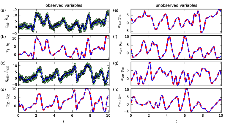
Figure 1: Adaption of the 80 dimensional Lorenz96 model (Eq. (16)) to the time series $\{\boldsymbol{\eta}(t_{n})\}$ (Eq. (17), green circles). Every second model variable was observed. Left-hand side: The model output given by the measurement function $\boldsymbol{h}(t)$ (Eq. (22), blue lines) was adapted to $\{\boldsymbol{\eta}(t_{n})\}$ ((a),(c)). (b) and (d) show the “true” solution $x_{i}$ (red dashed lines) with the corresponding estimates $y_{i}$ (blue lines),whereas for these quantities there exist measurements $\eta_{yi}$. Right-hand side: (e), (f), (g) and (h) show estimates for the model variables $y_{i}$ (blue lines) and the “true” solutions $x_{i}$ (red dashed lines). Note that for all cases shown on the right-hand side there exist no measurements. The model parameter is estimated to $p=8.165$, whereas $8.17$ is used for generating the data by (17). Note that only a few of the 80 estimated model variables (with and without data) are shown.

One can see a good coincidence of the model variables $\boldsymbol{y}(t)$ on the one hand and the “true” solution $\boldsymbol{x}(t)$ on the other hand. This is also the case for the observations $\{\boldsymbol{\eta}(t_{n})\}$ and $\boldsymbol{h}(\boldsymbol{y}(t))$. Furthermore the modeling error $\boldsymbol{u}(t)$ is small.

5 Delay differential equations and the estimation of delay parameters

An application where the cost function becomes rather complex and automatic differentiation turns out to be beneficial is the estimation of parameters and states of DDEs. How to derive the delayed variable $\boldsymbol{y}_{k}(n)=\boldsymbol{y}(n-k)$ from $\boldsymbol{y}(n)$ for $\tau=k\cdot\Delta t$ with $k\in\mathbb{N}$ was already discussed in Section 2.1. In this case ${\cal{Y}}_{k}(0,N)$ can be computed from ${\cal{Y}}(0,N)$ without interpolation. However, if $k\in\mathbb{R}_{+}$ this approach does not work anymore. One has to interpolate ${\cal{Y}}(0,N)$ to approximate ${\cal{Y}}_{k}(0,N)$. Because $\Delta t$ will be small a linear interpolation should be sufficient and hence is used here.

In the general case we have $\tau=(k^{\prime}+l)\cdot\Delta t$ with $\tau\in\mathbb{R}_{+}$, $k^{\prime}\in\mathbb{N}$ and $l\in[0,1[$. Note that, due to these restrictions on $k^{\prime}$ and $l$, $k^{\prime}$ and $l$ are uniquely defined for a given $\tau$. Using this substitution for $\tau$ the delayed variable can be written as

$$\boldsymbol{y}_{k}(n) =\boldsymbol{y}_{\tau}(t_{n})$$

$$=\boldsymbol{y}(t_{n}-\tau)$$

$$=\boldsymbol{y}(t_{n}-(k^{\prime}+l)\cdot\Delta t)$$

$$=\boldsymbol{y}(n\cdot\Delta t-(k^{\prime}+l)\cdot\Delta t)$$

$$=\boldsymbol{y}((n-k^{\prime}+l)\cdot\Delta t)$$

$$=\boldsymbol{y}(n-k^{\prime}+l)$$ (23)

and with linear interpolation between $\boldsymbol{y}(n-k^{\prime})$ and $\boldsymbol{y}(n-k^{\prime}+1)$ we obtain

$$\boldsymbol{y}_{k}(n) =\boldsymbol{y}(n-k^{\prime}+l)$$

$$=\boldsymbol{y}(n-k^{\prime})+\frac{\boldsymbol{y}(n-k^{\prime}+1)-\boldsymbol{y}(n-k^{\prime})}{\Delta t}\cdot l\cdot\Delta t$$

$$=\boldsymbol{y}(n-k^{\prime})+\left[\boldsymbol{y}(n-k^{\prime}+1)-\boldsymbol{y}(n-k^{\prime})\right]\cdot l$$ (24)

with $\boldsymbol{y}_{k}(n)\in[\boldsymbol{y}(n-k^{\prime}),\boldsymbol{y}(n-k^{\prime}+1)]$ for $n=0,1,\dots,N$. Note, that for $l=0$ we have $\tau=k^{\prime}\cdot\Delta t$ and hence the same situation as in Section 2.1, were $\boldsymbol{y}_{k}(n)=\boldsymbol{y}(n-k^{\prime})$ can be computed without an interpolation of the model variables.

One possibility to estimate $\tau$ is discussed now. First, $\tau$ must be added in Eq. (12) to the quantities to be estimated. Next, bounds for $\tau$ must be set in Eq. (9). This means that there are bounds to $k^{\prime}$ so that (if the smallest bound of $\tau$ is zero) we have $k^{\prime}\in[1,K]$. If $\tau$ and therefore $k^{\prime}$ and $l$ would be fixed and not estimated, $\boldsymbol{w}$ (Eq. (12)) would be $\boldsymbol{w}=({\cal{Y}}(-k^{\prime},N),\boldsymbol{p},\boldsymbol{q})$. When $\tau$ will be estimated, the number of elements in the history ${\cal{Y}}(-k^{\prime},-1)$ can vary during the optimization process due to variations in $\tau$ (performed by the optimizer) and in $k^{\prime}$. Because the number of elements of $\boldsymbol{w}$ has to stay constant during one optimization process, the history with the largest possible number of elements, given by ${\cal{Y}}(-K,-1)$, must be added to $\boldsymbol{w}$, which then becomes $\boldsymbol{w}=({\cal{Y}}(-K,N),\boldsymbol{p},\boldsymbol{q},\tau)$. Estimating $\tau$ with this approach has one major disadvantage. When the optimizer evaluates the cost function with a certain $\tau$, first $k^{\prime}$ and $l$ have to be derived from $\tau$. Next $k^{\prime}$ is used as an index to define the intervals $[\boldsymbol{y}(n-k^{\prime}),\boldsymbol{y}(n-k^{\prime}+1)]$ with $n=0,1,\dots N$ where to interpolate the model variables for deriving the delayed variables $\boldsymbol{y}_{k}(n)$ with $n=0,1,\dots N$. The cost function depends on the model equations, the model equations depend on the delayed variable and the delayed variable is, as shown in Eq. (24), a function of the model variables. Only the latter ones are quantities to be estimated. Hence the (sparse) Jacobian $\partial H_{i}(\boldsymbol{w})/\partial w_{j}$ of $\boldsymbol{H}(\boldsymbol{w})$ (see Eq. (15)) depends on the (sparse) Jacobian $\partial\boldsymbol{y}_{k}(n)/\partial\boldsymbol{y}(n)$ of the delayed variables to the model variables. For any specific $n$ there exist $K$ possible intervals $[\boldsymbol{y}(n-\tilde{k}),\boldsymbol{y}(n-\tilde{k}+1)]$ with $\tilde{k}\in[1,K]$ where the linear interpolation might be performed although there is only the one interval with $\tilde{k}=k^{\prime}$ where it finally will be performed. The derivative of the linear interpolation to the model variable can be written as $\partial\boldsymbol{y}_{k}(n)/\partial\boldsymbol{y}(n)=\partial\boldsymbol{y}_{(\tilde{k}+l)\Delta t}(n)/\partial\boldsymbol{y}(n)$ with $\tilde{k}=0,1,\dots,N$. Since only for $\tilde{k}=k^{\prime}$ a linear interpolation is performed, the relevant elements of the Jacobian matrix corresponding to $\tilde{k}\neq k$ are zero. Nevertheless, these elements which are zero at this step are not necessarily zero during the entire optimization process. Therefore these elements must be included in the sparsity pattern of nonzero elements, although, most of the time, they are zero. The sparsity pattern must not change during an optimization process. This fact would lead to a significant increase of (possible) nonzero elements in the Jacobian and hence would remove the advantage of dealing with a sparse Jacobian.

To avoid these problems the estimation of the delay parameter is divided into two steps:

First step:

The cost function is minimized for several fixed delays, $\tau=k\cdot\Delta t$ with $k\in\mathbb{N}$. In this case, as described in Section 2.1, no interpolation is necessary for computing the delayed variable. The solution of this step is $\hat{C}(\tau)$. This means that the assigned value is the value of the cost function in its minimum for a given $\tau$. $\hat{C}(\tau)$ has a global minimum close to $\tau_{\mathrm{min}}=k_{\mathrm{min}}\cdot\Delta t$.

Second step:

From the first step we have values for the cost function only around the minimum at $\tau_{\mathrm{min}}-\Delta t$, $\tau_{\mathrm{min}}$ and $\tau_{\mathrm{min}}+\Delta t$, as illustrated in Fig. 2. The global minimum at $\hat{\tau}$ is either in the interval $\hat{\tau}\in[\tau_{\mathrm{min}}-\Delta t,\tau_{\mathrm{min}}]$ or in the interval $\hat{\tau}\in[\tau_{\mathrm{min}},\tau_{\mathrm{min}}+\Delta t]$. Now, $\tau$ is estimated as well. As described at the beginning of this section, the delayed variable is computed by linear interpolation of the model variable. The cost function is minimized two times: once with $\tau\in[\tau_{\mathrm{min}}-\Delta t,\tau_{\mathrm{min}}]$ and then with $\tau\in[\tau_{\mathrm{min}},\tau_{\mathrm{min}}+\Delta t]$. The solution (model variables, parameters, delay time) obtained for the interval with the smallest value of the cost function after the optimization procedure is then taken as the final solution.

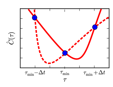
Figure 2: Estimation of the delay parameter: An illustration of the cost function $\hat{C}(\tau)$ around the minimum at $\tau_{\mathrm{min}}$ is shown. The values of $\hat{C}(\tau)$ shown by the (blue) dots where obtained by the first step of estimating the delay parameter. The global minimum of $\hat{C}(\tau)$ at $\hat{\tau}$ is either in the interval $\hat{\tau}\in[\tau_{\mathrm{min}}-\Delta t,\tau_{\mathrm{min}}]$ or in the interval $\hat{\tau}\in[\tau_{\mathrm{min}},\tau_{\mathrm{min}}+\Delta t]$, as illustrated by the (red) dashed and continuous lines. Both lines describe possible behaviors of $\hat{C}(\tau)$ between the (blue) dots. To determine whether the global minimum is in $[\tau_{\mathrm{min}}-\Delta t,\tau_{\mathrm{min}}]$ or $[\tau_{\mathrm{min}},\tau_{\mathrm{min}}+\Delta t]$ both intervals are investigated separately in the second step using linear interpolation of the state variable.

6 Example: Mackey-Glass model

As an example of a DDE we consider the Mackey-Glass model [29]. This time delay model is given by

$$\frac{\mathrm{d}y(t)}{\mathrm{d}t} =p_{1}\cdot\frac{y(t-\tau)}{1+y(t-\tau)^{10}}-p_{2}y(t)$$ (25)

and has the two model parameters $p_{1}$, $p_{2}$ beside the delay parameter $\tau$. To generate a data time series a twin experiment is performed. This means that the model (similar to Eq. (25))

$$\frac{\mathrm{d}x(t)}{\mathrm{d}t} =2\cdot\frac{x(t-2.38)}{1+x(t-2.38)^{10}}-1\cdot x(t)$$ (26)

was integrated first. The solution is then used to generate the (noisy) time series

$$\eta(t_{n}) =x(t_{n})+\mathcal{N}(0,0.1)$$ (27)

with $t_{n}\in\{0,0.1,\dots,60\}$ and $N=601$ with timesteps $\Delta t=0.1$ ($\mathrm{SNR}=8.0\mathrm{dB}$ according to Eq. (20)).

Next the model (25) was adapted to $\{\eta(t_{n})\}$ using the measurement function

$$h(y(t),\bullet,\bullet) =y(t)\,.$$ (28)

The parameters $p_{1}$, $p_{2}$ and $\tau$ were estimated in addition to the model variable. As described in Section 5 the estimation of $\tau$ is divided into two steps:

• First $\tau$ is fixed to several different values $\tau=k\cdot\Delta t$ with $k=3,4,\dots,100$ and $\Delta t=0.1$. For each fixed $\tau$ the cost function is minimized. The value of the cost function at its minimum is denoted by $\hat{C}(\hat{{\cal{Y}}}(-k,N),\hat{\boldsymbol{p}},\bullet,\tau)$. Its dependence on $\tau$ is shown in Fig. 3. One can see a clear minimum at $\tau=2.3$. Due to the step size of $\Delta t=0.1$ and the smoothness around this minimum one can expect that the global minimum is either at $\tau\in[2.2,2.3]$ or at $\tau\in[2.3,2.4]$.

• Second the cost function is minimized two times (first with the bounds $\tau\in[2.2,2.3]$ and second with $\tau\in[2.3,2.4]$). In each case the delayed variable is approximated by linear interpolation according to Eq. (24). Remember that due to the bounds the index $k^{\prime}$ does not change during each optimization process and hence does not have to be recomputed from $\tau$ in each iteration. Only $l$ changes.

For all performed estimation processes the weighting matrices of the cost function (5) (in this cases they are scalar) and $\alpha$ were fixed to: $A=B=1$, $E=10^{3}$, $\beta=10^{5}$ and $\alpha=0.5$. The results for the estimated parameters and the delay parameter are shown in tab. 2.

×	$(p_{1},p_{2})$	$\tau$	$\hat{C}(\dots,\tau)$
data	$(2,1)$	2.38	×
estim. $\tau\in[2.2,2.3]$	$(1.73,0.86)$	2.300	$5.41\cdot 10^{-3}$
estim. $\tau\in[2.3,2.4]$	$(1.98,0.99)$	2.387	$4.99\cdot 10^{-3}$

Table 2: Model parameters $p_{1}$, $p_{2}$ and delay parameter $\tau$ of the Mackey-Glass model (25) estimated by adapting the model (25) to the time series given by Eq. (27). According to Fig. 3 the cost function $\hat{C}(\hat{{\cal{Y}}}(-k,N),\hat{\boldsymbol{p}},\bullet,\tau)$ has its global minimum either in $\tau\in[2.2,2.3]$ or in $\tau\in[2.3,2.4]$. Minimizing the cost function and estimating $\tau$ in addition to the model parameters and variables for both intervals results in a smaller $\hat{C}(\hat{{\cal{Y}}}(-k,N),\hat{\boldsymbol{p}},\bullet,\tau)$ for $\tau\in[2.3,2.4]$.

Figure 3: Cost function for adaption of the Mackey-Glass (25) model to a time series generated in a twin experiment with Eq. (27).

For $\tau\in[2.3,2.4]$ the cost function $\hat{C}(\dots,\tau)$ at its minimum has a smaller value than for $\tau\in[2.2,2.3]$. Hence the solution for $\tau\in[2.3,2.4]$ was chosen as the final result. Furthermore the estimated values for $p_{1}$, $p_{2}$ and $\tau$ coincide much better with the “true” values used to generate $\{\eta(t_{n})\}$ (compared to the estimated values with $\tau\in[2.2,2.3]$). The estimated model variable for $\tau\in[2.3,2.4]$ is shown in Fig. 4.

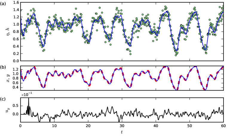
Figure 4: Adaption of the Mackey-Glass (25) model to the time series $\eta$ (see (27) green circles) which was generated by the original “true” solution $x$ red dashed line,) unknown to the estimation algorithm) using the measurement function $h(y(t),\bullet,\bullet)$ (blue line, see (28)). The estimated solution for the model variable is $y$ (blue line in (b)) and $u$ (black line in (c)) is the error in the approximation of the model equation (see (4)). The delay time $\tau\in[2.3,2.4]$ was also estimated beside the model parameters and all estimated values are shown in tab. 2.

One can see a good coincidence of the model variable $y(t)$ on the one hand and the “true” solution $x(t)$ (Fig. 4b) and the data $\{\eta(t_{n})\}$ (Fig. 4a) on the other hand with a small modeling error $u(t)$ (Fig. 4c).

7 Conclusion

Many optimization based system identification methods require information about derivatives of the underlying cost function in order to converge to the desired optimum. In general this information has to be provided by the user (or programmer) in terms of a Jacobian matrix, for example. Our examples show that this (typically cumbersome) task can be conveniently handled by means of automatic differentiation. This versatile tool from applied mathematics and computer science not only gives exact numerical values of the required derivatives, but also provides (and respects) the sparsity structure of the Jacobian matrix which may be exploited by any calling algorithm. These features have been demonstrated with a particular optimization algorithm (SparseLM) that enabled parameter and state estimation of the high dimensional Lorenz-96 system and the Mackey-Glass delay differential equation. A challenge for future research will be, for example, a successful application of the proposed parameter estimation to electrophysiological models of cardiac myocytes.

Our implementation (Python, C) of the estimation algorithm and a Python wrapper for sparseLM are available for download [32]. Other possible fields of application in nonlinear dynamics are bifurcation analysis and the computation of Lyapunov exponents and (covariant) Lyapunov vectors [33].

Appendix A Python example for automatic differentiation using ADOL-C

For illustration we present and discuss a Python example showing how to derive the sparse Jacobian of a function $\boldsymbol{H}(\boldsymbol{w})$ in Listing 1.

Listing 1: Simple Python example demonstrating the derivation of the (sparse) Jacobian of the function $\boldsymbol{H}(\boldsymbol{w})$ usind the automatic differentiation tool ADOL-C.

⬇

1import numpy as np

2import adolc

3

4def H(w):

5 h = np.zeros(3,dtype=w.dtype)

6 h[0] = 3*w[0]**2 + w[1]*w[3]

7 h[1] = 4*w[2]**3

8 h[2] = 5*w[0] + 2*np.exp(np.sin(w[1]*w[2]))

9 return h

10

11w0 = np.array([4.,2.,3.,1.])

12

13# Trace H(w)

14# ———-

15adolc.trace_on(0)

16aw = adolc.adouble(w0)

17adolc.independent(aw)

18

19Hfunc = H(aw)

20

21adolc.dependent(Hfunc)

22adolc.trace_off()

23

24# Evaluate function jacobian at this point

25w = np.array([-2.,3.,1.,-4.])

26

27# Evaluate function

28valH = adolc.function(0,w)

29

30# Evaluate dense jacobian

31jacH = adolc.jacobian(0,w)

32# Out jacH:

33# [[-12. -4. 0. 3.]

34# [ 0. 0. 12. 0.]

35# [ 5. -2.280 -6.840 0.]]

36

37# Derive sparsity pattern and evaluate values of nonzeros at w0

38# ————————————————————-

39options = [0, 0, 0, 0]

40[nnz, rind, cind, val] = adolc.colpack.sparse_jac_no_repeat(0,w0,options)

41# Out nnz (number non-zeros): 7

42# Out rind (row indices):

43# [0 0 0 1 2 2 2]

44# Out cind (column indices):

45# [0 1 3 2 0 1 2]

46# Out val (values):

47# [ 24. 1. 2. 108. 5. 4.356 2.904]

48

49# Evaluate values of nonzeros at w using nnz,

50# rind, cind and valH from the previous step

51# ——————————————-

52[nnz, rind, cind, val] = adolc.colpack.sparse_jac_repeat(0,w,nnz, rind,cind,val)

53# Out nnz (number non-zeros): 7

54# Out rind (row indices):

55# [0 0 0 1 2 2 2]

56# Out cind (column indices):

57# [0 1 3 2 0 1 2]

58# Out val (values):

59# [-12. -4. 3. 12. 5. -2.280 -6.840]

Before ADOLC can compute the numerical values of the Jacobian data type an internal function representation of H(w), called trace, is created in lines 15-22. To do this the data type of the elements of the input vector is changed to the ADOL-C data type ’adouble’ (line 16). Many (mathematical) functions are overloaded for this data type and can hence be used in the function to be differentiated. FOR-loops, WHILE-loops, IF … THEN statements, etc. are also allowed under certain conditions. In lines 28 and 31 the function H(w) and its dense Jacobian are computed using the previously created trace for a new $\boldsymbol{w}$. In line 40 the sparsity pattern of the Jacobian is detected and used in line 52 to compute the numerical values of its non-zero elements. The output in lines 33-35 and lines 55-59 show that the computed dense and sparse Jacobians are equal for the same $\boldsymbol{w}$.

References

- [1] R.H. Clayton, O. Bernus, E.M. Cherry, H. Dierckx, F.H. Fenton, L. Mirabella, S.V. Panfilov, F.B. Sachse, G. Seeman, H. Zhang, Models of cardiac tissue electrophysiology: Progress, challenges and open questions, Prog. Biophys. Mol. Biol. 104, 22-48 (2011).
- [2] U. Parlitz, L. Junge and L. Kocarev, Synchronization based parameter estimation from time series, Phys. Rev. E 54, 6253-6529 (1996).
- [3] H. U. Voss, J. Timmer and J. Kurths, Nonlinear dynamical system identification from uncertain and indirect measurements, Int. J. Bifurcation and Chaos 14, 1905-1933 (2004)
- [4] D. Ghosh and S. Banerjee, Adaptive scheme for synchronization-based multiparameter estimation from a single chaotic time series and its applications, Phys. Rev. E 78, 056211 (2008).
- [5] H. D. I. Abarbanel, D.R. Creveling, J.M. Jeanne, Estimation of parameters in nonlinear systems using balanced synchronization, Phys. Rev. E 77, 016208 (2008).
- [6] F. Sorrentino and E. Ott, Using synchronization of chaos to identify the dynamics of unknown systems Chaos 19, 033108 (2009).
- [7] I. G. Szendro, M. A. Rodríguez and J. M. López, On the problem of data assimilation by means of synchronization, J. Geophys. Res. 114, D20109 (2009).
- [8] W. Yu, G. Chen, J. Cao, J. Lü and U. Parlitz, Parameter identification of dynamical systems from time series, Phys. Rev. E 75, 067201 (2007).
- [9] D. Yu and U. Parlitz, Estimating parameters by autosynchronization with dynamic restrictions, Phys. Rev. E 77, 066221 (2008).
- [10] D. Ghosh, Nonlinear-observerÐbased synchronization scheme for multiparameter estimation, EPL 84, 40012 (2008).
- [11] D. Fairhurst, I. Tyukin, H. Nijmeijer and C. van Leeuwen, Observers for Canonic Models of Neural Oscillators, Math. Model. Nat. Phenom. 5(3), 146-185 (2010).
- [12] D.R. Creveling, P.E. Gill, H. D. I. Abarbanel, State and parameter estimation in nonlinear systems as an optimal tracking problem, Phys. Lett. A 372, 2640-2644 (2008).
- [13] J.C. Quinn, P.H. Bryant, D. R. Creveling, S. R. Klein, and H. D. I. Abarbanel, Parameter and state estimation of experimental chaotic systems using synchronization, Phys. Rev. E 80, 016201 (2009).
- [14] H. D. I. Abarbanel, D. R. Creveling, R. Farsian and M. Kostuk, Dynamical State and Parameter Estimation, SIAM J. Appl. Dyn. Syst. 8, 1341-1381 (2009).
- [15] H.D.I. Abarbanel,Effective actions for statistical data assimilation, Phys. Lett. A 373, 4044 404 (2009).
- [16] J.C. Quinn, H.D.I. Abarbanel, State and parameter estimation using Monte Carlo evaluation of path integrals, Q. J. R. Meteorol. Soc. 136 (652), 1855-1867 (2010).
- [17] H.D.I. Abarbanel, M. Kostuk and W. Whartenby, Data assimilation with regularized nonlinear instabilities, Q J. R. Meteorol. Soc. 136 (648), 769- 783 (2010).
- [18] J. Bröcker, On Variational Data Assimilation in Continuous Time, Q. J. R. Meteorol. Soc. 136, 1906-1919 (2010).
- [19] J. Schumann-Bischoff and U. Parlitz, State and parameter estimation using unconstrained optimization, Phys. Rev. E 84, 056214 (2011).
- [20] J. Bröcker and I. Szendro Sensitivity And Out–Of–Sample Error of Continuous Time Data Assimilation, Q. J. R. Meteorol. Soc. 138, 785-801 (2012).
- [21] K. Levenberg, A Method for the Solution of Certain Problems in Least Squares, Quart. Appl. Math. 2, 164-168 (1944).
- [22] D. Marquardt, An Algorithm for Least-Squares Estimation of Nonlinear Parameters, SIAM J. Appl. Math. 11, 431-441 (1963).
- [23] M. I. A. Lourakis, Sparse Non-linear Least Squares Optimization for Geometric Vision, European Conference on Computer Vision 2, 43-56 (2010). http://dx.doi.org/10.1007/978-3-642-15552-9_4 and http://www.ics.forth.gr/~lourakis/sparseLM/
- [24] L. B. Rall, Automatic Differentiation: Techniques and Applications, Lecture Notes in Computer Science 120 (1981).
- [25] A. Walther and A. Griewank, Getting started with ADOL-C, in U. Naumann and O. Schenk, Combinatorial Scientific Computing, Chapman-Hall CRC Computational Science, 181-202 (2012).
- [26] A. Griewank, D. Juedes and J. Utke, Algorithm 755: ADOL-C: A Package for the Automatic Differentiation of Algorithms Written in C/ C++, ACM Trans. on Math. Softw. 22, 131-167 (1996).
- [27] ColPack: http://www.cscapes.org/coloringpage/software.htm (accessed: October 16, 2012)
- [28] E. N. Lorenz, Predictability – A problem partly solved, ECMWF, Reading, Berkshire, UK, Proceedings of the Seminar on Predictability 1, 1-18 (1996).
- [29] M. C. Mackey and L. Glass, Oscillation and chaos in physiological control systems, Science 197, 287-289 (1977).
- [30] Numpy: http://numpy.scipy.org/ (accessed: October 16, 2012)
- [31] Pyadolc: https://github.com/b45ch1/pyadolc (accessed: October 16, 2012)
- [32] A Python wrapper for sparseLM and a Python-C implementation of the estimation method for ODEs can be downloaded from http://www.bmp.ds.mpg.de/pysparselm.html and http://www.bmp.ds.mpg.de/pyodefit.html (Gnu General Public License Version 3, 29 June 2007)
- [33] P.V. Kuptsov and U. Parlitz, Theory and Computation of Covariant Lyapunov Vectors, J. Nonlinear Sci. 22, 727-762 (2012).