Controlling the stability of steady states in continuous variable quantum systems

Abstract

For the paradigmatic case of the damped quantum harmonic oscillator we present two measurement-based feedback schemes to control the stability of its fixed point. The first scheme feeds back a Pyragas-like time-delayed reference signal and the second uses a predetermined instead of time-delayed reference signal. We show that both schemes can reverse the effect of the damping by turning the stable fixed point into an unstable one. Finally, by taking the classical limit $\hbar\rightarrow 0$ we explicitly distinguish between inherent quantum effects and effects, which would be also present in a classical noisy feedback loop. In particular, we point out that the correct description of a classical particle conditioned on a noisy measurement record is given by a non-linear stochastic Fokker-Planck equation and not a Langevin equation, which has observable consequences on average as soon as feedback is considered.

1 Introduction

Continuous variable quantum systems are quantum systems whose algebra is described by two operators $\hat{x}$ and $\hat{p}$ (usually called position and momentum), which obey the commutation relation $[\hat{x},\hat{p}]=i\hbar$. Such systems constitute an important class of quantum systems. They do not only describe the quantum mechanical analogue of the motion of classical heavy particles in an external potential, but they also arise, e.g., in the quantization of the electromagnetic field. Understanding them is important, e.g., in quantum optics ScullyZubairyBook1997 , for purposes of quantum information processing BraunsteinVanLoockRMP2005 ; WeedbrookEtAlRMP2012 , or in the growing field of optomechanics AspelmeyerKippenbergMarquardtRMP2014 . Furthermore, due to the pioneering work of Wigner and Weyl, such systems have a well-defined classical limit and can be used to understand the transition from the quantum to the classical world FaddeevYakubovskiiBook2009 .

To each quantum system there is an operator associated, called the Hamiltonian $\hat{H}$, which describes its energy and determines the dynamics of the system if it is isolated. However, in reality each system is an open system, i.e., it interacts with a large environment (we call it the bath). Since the bath is so large that we cannot describe it in detail, it induces effects like damping, dissipation or friction, which will eventually bring the system to a steady state. Classically as well as quantum mechanically it is often important to be able to counteract such irreversible behaviour, for instance, by applying a suitably designed feedback loop.

In the quantum domain, however, feedback control faces additional challenges compared to the classical world WisemanMilburnBook2010 , see also Fig. 1. Each closed loop control scheme starts by measuring a certain output of the system and tries to feed the so gained information back into the system by adjusting some system parameters to influence its dynamics. In the quantum world – due to the measurement postulate of quantum mechanics and the associated “collapse of the wavefunction” – the measurement itself significantly disturbs the system and thus, it already influences the dynamics of the system. If one does not take this fact correctly into account, one easily arrives at wrong conclusions. Nevertheless, beautiful experiments have shown that quantum feedback control is invaluable to protect quantum information and to stabilize non-classical states of light and matter in various settings, see e.g. Refs. SmithEtAlPRL2002 ; BushevEtAlPRL2006 ; GillettEtAlPRL2010 ; HarocheNature2011 ; VijayEtAlNature2012 ; RisteEtAlPRL2012 for a selection of pioneering work in this field.

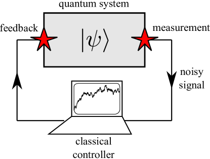
Figure 1: Generic sketch for a closed-loop feedback scheme, in which we wish to control the dynamics of a given quantum system. Note that the feedback loop itself is actuated by a classical controller, i.e., the information after the measurement is classical (it is a number and not an operator). Nevertheless, to obtain the correct dynamics of the quantum system one needs to pay additional attention to the measurement and feedback step.

In this contribution we will apply two measurement based control schemes to a simple quantum system, the damped harmonic oscillator (HO), by correctly taking into account measurement and feedback noise at the quantum level (Sec. 3 and 4). These schemes will reverse the effect of dissipation and – to the best of our knowledge – have not been considered in this form elsewhere. However, we will see that our treatment is conceptually very close to a classical noisy feedback loop. With this contribution we thus also hope to provide a bridge between quantum and classical feedback control. For pedagogical reasons we will therefore first present the necessary technical ingredients (continuous quantum measurement theory, quantum feedback theory and the phase space formulation of quantum mechanics) in Sec. 2. Due to a limited amount of space we cannot derive them here, but we will try to make them as plausible as possible. Sec. 5 is then devoted to a thorough discussion of the classical limit of our results showing which effects are truly quantum and which can be also expected in a classical feedback loop. In the last section we will give an outlook about possible applications and extensions of our feedback loop.

2 Preliminary

2.1 The damped quantum harmonic oscillator

We will focus only on the damped HO in this paper, but we will discuss extensions and applications of our scheme to other systems in Sec. 6. Using a canonical transformation we can rescale position and momentum such that the Hamiltonian of the HO reads $\hat{H}=\omega(\hat{p}^{2}+\hat{x}^{2})/2$ with $[\hat{x},\hat{p}]=i\hbar$. Introducing linear combinations of position and momentum, called the annihilation operator $\hat{a}\equiv(\hat{x}+i\hat{p})/\sqrt{2\hbar}$ and its hermitian conjugate, the creation operator $\hat{a}^{\dagger}$, we can express the Hamiltonian as $\hat{H}=\hbar\omega(\hat{a}^{\dagger}\hat{a}+1/2)$. Note that we explicitly keep Planck’s contant $\hbar$ to take the classical limit ($\hbar\rightarrow 0$) later on.

The state of the HO is described by a density matrix $\hat{\rho}$, which is a positive, hermitian operator with unit trace: $\mbox{tr}\hat{\rho}=1$. If the HO is coupled to a large bath of different oscillators at a temperature $T$, it is possible to derive a so-called master equation (ME) for the time evolution of the density matrix ScullyZubairyBook1997 ; WisemanMilburnBook2010 ; CarmichaelBook1993 :

$$\frac{\partial}{\partial t}\hat{\rho}(t)=-\frac{i}{\hbar}[\hat{H},\hat{\rho}(t)]+\kappa(1+n_{B}){\cal{D}}[\hat{a}]\hat{\rho}(t)+\kappa n_{B}{\cal{D}}[\hat{a}^{\dagger}]\hat{\rho}(t).$$ (1)

Here, we introduced the dissipator ${\cal{D}}$, which is defined for an arbitrary operator $\hat{o}$ by its action on the density matrix: $D[\hat{o}]\hat{\rho}\equiv\hat{o}\hat{\rho}\hat{o}^{\dagger}-\{\hat{o}^{\dagger}\hat{o},\hat{\rho}\}/2$ where $\{\hat{a},\hat{b}\}\equiv\hat{a}\hat{b}+\hat{b}\hat{a}$ denotes the anti-commutator. Furthermore, $\kappa>0$ is a rate of dissipation characterizing how strong the time evolution of the system is effected by the bath and $n_{B}$ denotes the Bose-Einstein distribution, $n_{B}\equiv(e^{\beta\hbar\omega}-1)^{-1}$, where $\beta\equiv 1/T$ is the inverse temperature (we set $k_{B}\equiv 1$). For later purposes we abbreviate the whole ME (1) by

$$\frac{\partial}{\partial t}\hat{\rho}(t)\equiv{\cal{L}}_{0}\hat{\rho}(t),$$ (2)

where the “superoperator” ${\cal{L}}_{0}$ is often called the Liouvillian and the subscript $0$ refers to the fact that this is the ME for the free time evolution of the HO without any measurement or feedback performed on it. Furthermore, it will turn out to be convenient to introduce a superoperator notation for the commutator and anti-commutator:

$${\cal{C}}[\hat{o}]\hat{\rho}\equiv[\hat{o},\hat{\rho}],~{}~{}~{}{\cal{A}}[\hat{o}]\hat{\rho}\equiv\{\hat{o},\hat{\rho}\}.$$ (3)

One easily verifies that the time evolution of the expectation values of position ${\langle{\hat{x}}\rangle}(t)\equiv\mbox{tr}\{\hat{x}\hat{\rho}(t)\}$ and momentum ${\langle{\hat{p}}\rangle}(t)\equiv\mbox{tr}\{\hat{p}\hat{\rho}(t)\}$ is

$$\begin{split}\frac{d}{dt}{\langle{x}\rangle}(t)&=\omega{\langle{p}\rangle}(t)-\frac{\kappa}{2}{\langle{x}\rangle}(t),\\ \frac{d}{dt}{\langle{p}\rangle}(t)&=-\omega{\langle{x}\rangle}(t)-\frac{\kappa}{2}{\langle{p}\rangle}(t),\end{split}$$ (4)

as for the classical damped harmonic oscillator. More generally speaking, for an arbitrary dynamical system these equations describe the generic situation for a two-dimensional stable steady state $(x^{*},p^{*})=(0,0)$ within the linear approximation around $(0,0)$. For $\kappa<0$ this would describe an unstable steady state, but physically we can only allow for positive $\kappa$. The positivity of $\kappa$ is mathematically required by Lindblad’s theorem LindbladCMP1976 ; GoriniEtAlJMP1976 to guarantee that Eq. (1) describes a valid time evolution of the density matrix.

Finally, a reader unfamiliar with this subject might find it instructive to verify that the canonical equilibrium state

$$\hat{\rho}_{\text{eq}}\sim e^{-\beta\hat{H}}\sim e^{-\beta\hbar\omega\hat{a}^{\dagger}\hat{a}}$$ (5)

is a steady state of the total ME (1) as it is expected from arguments of equilibrium statistical mechanics.

2.2 Continuous quantum measurements

In introductory courses on quantum mechanics (QM) one only learns about projective measurements, which yield the maximum information but are also maximally invasive in the sense that they project the total state $\hat{\rho}$ onto a single eigenstate. QM, however, also allows for much more general measurement procedures WisemanMilburnBook2010 . For our purposes, so-called continuous quantum measurements are most suited. They arise by considering very weak (i.e., less invasive) measurements, which are repeatedly performed on the system. In the limit where the time between two measurements goes to zero and the measurement becomes infinitely weak, we end up with a continuous quantum measurement scheme. For a quick introduction see Ref. JacobsSteckContempPhys2006 . Using their notation, one needs to replace $k\mapsto\gamma/(4\hbar)$ to obtain our results.

For our purposes we want to continuously measure (or “monitor”) the position of the HO. Details of how to model the system-detector interaction can be found elsewhere BarchielliLanzProsperiNuovoCim1982 ; BarchielliLanzProsperiFoundPhys1983 ; CavesMilburnPRA1987 ; WisemanMilburnPRA1993 ; DohertyJacobsPRA1999 . Here, we restrict ourselves to showing the results and we try to make them plausible afterwards. If we neglect any contribution from ${\cal{L}}_{0}$ for the moment, the time evolution of the density matrix due to the measurement of $\hat{x}$ is WisemanMilburnBook2010 ; JacobsSteckContempPhys2006 ; BarchielliLanzProsperiNuovoCim1982 ; BarchielliLanzProsperiFoundPhys1983 ; CavesMilburnPRA1987 ; WisemanMilburnPRA1993 ; DohertyJacobsPRA1999

$$\frac{\partial}{\partial t}\hat{\rho}(t)=-\frac{\gamma}{4\hbar}{\cal{C}}^{2}[\hat{x}]\hat{\rho}(t)\equiv{\cal{L}}_{\text{meas}}\hat{\rho}(t).$$ (6)

Here, the new parameter $\gamma$ has the physical dimension of a rate and quantifies the strength of the measurement. For $\gamma=0$ we thus recover the case without any measurement. It is instructive to have a look how the matrix elements of $\hat{\rho}(t)$ evolve in the measurement basis $|x\rangle$ of the position operator $\hat{x}=\int dxx|x\rangle\langle x|$:

$$\frac{\partial}{\partial t}\langle x|\hat{\rho}(t)|x^{\prime}\rangle=-\frac{\gamma}{4\hbar}(x-x^{\prime})^{2}\langle x|\hat{\rho}(t)|x^{\prime}\rangle.$$ (7)

We thus see that the off-diagonal elements (or “coherences”) are exponentially damped whereas the diagonal elements (or “populations”) remain unaffected. This is exactly what we would expect from a weak quantum measurement: the density matrix is perturbed only slightly but finally, in the long-time limit, it becomes diagonal in the measurement basis. Note that in case of a standard projective measurement scheme, the coherences would instantaneously vanish.

The ME (6) is, however, only half of the story, because it tells us only about the average time evolution of the system, i.e., about the whole ensemble $\hat{\rho}$ averaged over all possible measurement records. The distinguishing feature of closed-loop control (as compared to open-loop control) is, however, that we want to influence the system based on a single (and not ensemble) measurement record. We denote the density matrix conditioned on a certain measurement record by $\hat{\rho}_{c}$ and call it the conditional density matrix. Its classical counterpart would be simply a conditional probability distribution.

In QM, even in absence of classical measurement errors, each single measurement record is necessarily noisy due to the inherent probabilistic interpretation of measurement outcomes in QM. The measurement signal $I(t)$ associated to the continuous position measurement scheme above can be shown to obey the stochastic process WisemanMilburnBook2010 ; JacobsSteckContempPhys2006

$$dI(t)=\langle\hat{x}\rangle_{c}(t)dt+\sqrt{\frac{\hbar}{2\gamma\eta}}dW(t).$$ (8)

Here, by $\langle\hat{x}\rangle_{c}(t)$ we denoted the expectation value with respect to the conditional density matrix, i.e., $\langle\hat{x}\rangle_{c}(t)\equiv\mbox{tr}\{\hat{x}\hat{\rho}_{c}(t)\}$. Furthermore, $dW(t)$ is the Wiener increment. According to the standard rules of stochastic calculus, it obeys the relations WisemanMilburnBook2010 ; JacobsSteckContempPhys2006

$$\mathbb{E}[dW(t)]=0,~{}~{}~{}dW(t)^{2}=dt$$ (9)

where $\mathbb{E}[\dots]$ denotes a (classical) ensemble average over all noisy realizations. Furthermore, we have introduced a new parameter $\eta\in[0,1]$, which is used to model the efficiency of the detector WisemanMilburnBook2010 ; JacobsSteckContempPhys2006 ; WisemanMilburnPRA1993 with $\eta=1$ corresponding to the case of a perfect detector.

Finally, we need to know how the state of the system evolves conditioned on a certain measurement record. This evolution is necessarily stochastic due to the stochastic measurement record. The so-called stochastic ME (SME) turns out to be given by WisemanMilburnBook2010 ; JacobsSteckContempPhys2006

$$\hat{\rho}_{c}(t+dt)=\hat{\rho}_{c}(t)+{\cal{L}}_{\text{meas}}\hat{\rho}_{c}(t)dt+\sqrt{\frac{\gamma\eta}{2\hbar}}{\cal{A}}[\hat{x}-\langle\hat{x}\rangle_{c}(t)]\hat{\rho}_{c}(t)dW(t).$$ (10)

Because it will turn out to be useful, we have written the SME in an “incremental form” by explicitly using differentials as one would also do for numerical simulations. By definition we regard the quantity $[\hat{\rho}_{c}(t+dt)-\hat{\rho}_{c}(t)]/dt$ as being equivalent to $\partial_{t}\hat{\rho}_{c}(t)$. Using Eq. (8) we can express the SME alternatively as

$$\hat{\rho}_{c}(t+dt)=\hat{\rho}_{c}(t)+{\cal{L}}_{\text{meas}}\hat{\rho}_{c}(t)dt+\frac{\gamma\eta}{\hbar}{\cal{A}}[\hat{x}-\langle\hat{x}\rangle_{c}(t)]\hat{\rho}_{c}(t)[dI(t)-\langle\hat{x}\rangle_{c}(t)dt],$$ (11)

which explicitly demonstrates how our knowledge about the state of the system changes conditioned on a given measurement record $I(t)$. We remark that the SME for $\hat{\rho}_{c}(t)$ is nonlinear in $\hat{\rho}_{c}(t)$, due to the fact that this in an equation of motion for a conditional density matrix.

To obtain the ME (6) for the average evolution, we only need to average the SME (10) over all possible measurement trajectories. In fact, it can be shown (see WisemanMilburnBook2010 ; JacobsSteckContempPhys2006 ) that Eq. (10) has to be interpreted within the rules of Itô stochastic calculus (as well as all the following stochastic equations unless otherwise mentioned) such that

$$\mathbb{E}[\hat{\rho}_{c}(t)dW(t)]=\mathbb{E}[\hat{\rho}_{c}(t)]\mathbb{E}[dW(t)]=0$$ (12)

holds. Defining $\hat{\rho}(t)\equiv\mathbb{E}[\hat{\rho}_{c}(t)]$, one can readily verify that the SME (10) yields on average Eq. (6).

Taking the free evolution of the HO into account, Eq. (1), the total stochastic evolution of the system obeys

$$\hat{\rho}_{c}(t+dt)=\left\{1+({\cal{L}}_{0}+{\cal{L}}_{\text{meas}})dt+\sqrt{\frac{\gamma\eta}{2\hbar}}{\cal{A}}[\hat{x}-\langle\hat{x}\rangle_{c}(t)]dW(t)\right\}\hat{\rho}_{c}(t).$$ (13)

Note that there are no “mixed terms” from the free evolution and the evolution due to the measurement to lowest order in $dt$. Furthermore, we remark that a solution of a SME is called a quantum trajectory in the literature WisemanMilburnBook2010 ; CarmichaelBook1993 ; GardinerZollerBook2004 .

2.3 Direct quantum feedback

In the following we will consider a form of quantum feedback control, which is sometimes called direct quantum feedback control, because the measurement signal is directly fed back into the system (possibly with a delay) without any additional post-processing of the signal as, e.g., filtering or parameter estimation DohertyJacobsPRA1999 . Direct quantum feedback based on a continuous measurement scheme was developed by Wiseman and Milburn WisemanMilburnPRL1993 ; WisemanMilburnPRA1994 ; WisemanPRA1994 . Experimentally, the idea would be to continuously adjust a parameter of the Hamiltonian based on the measurement outcome (8) to control the dynamics of the system. Theoretically, we define the feedback control superoperator ${\cal{F}}$

$$[\dot{\rho}_{c}(t)]_{\text{fb}}={\cal{F}}\hat{\rho}_{c}(t)\equiv-\frac{i}{\hbar}\frac{dI(t)}{dt}{\cal{C}}[\hat{z}]\hat{\rho}_{c}(t),$$ (14)

which describes a change of the free system Hamiltonian $\hat{H}=\omega(\hat{p}^{2}+\hat{x}^{2})/2$ to a new effective Hamiltonian $\omega(\hat{p}^{2}+\hat{x}^{2})/2+\frac{dI(t)}{dt}\hat{z}$ containing a new term proportional to the measurement result and an arbitrary hermitian operator $\hat{z}$ (with units of $\dot{x}$). Here, we neglected any delay and assumed an instantaneous feedback of the measurement signal, but a delay can be easily incorporated, too, see Sec. 3.

Because the action of the feedback superoperator ${\cal{F}}$ on the system was merely postulated, we do not a priori know whether we have to interpret it according to the Itô or Stratonovich rules of stochastic calculus, but it turns out that only the latter interpretation gives senseful results WisemanMilburnBook2010 ; WisemanMilburnPRL1993 ; WisemanMilburnPRA1994 . Then, the effect of the feedback on the total time evolution of the system (including the measurement and free time evolution) can be found by exponentiating Eq. (14) WisemanMilburnBook2010 ; WisemanMilburnPRL1993 ; WisemanMilburnPRA1994

$$\hat{\rho}_{c}(t+dt)=e^{{\cal{F}}dt}\left\{1+{\cal{L}}_{0}dt+{\cal{L}}_{\text{meas}}dt+\sqrt{\frac{\gamma\eta}{2\hbar}}{\cal{H}}[\hat{x}]dW(t)\right\}\hat{\rho}_{c}(t)$$ (15)

and this equation is again of Itô type. Note that by construction this equation assures that the feedback step happens after the measurement as it must due to causality. Now, expanding $e^{{\cal{F}}dt}$ to first order in $dt$ with $dI(t)$ from Eq. (8) (note that this requires to expand the exponential function up to second order due to the contribution from $dW(t)^{2}=dt$) and using the rules of stochastic calculus gives the effective SME under feedback control:

$$\begin{split}\hat{\rho}_{c}(t+dt)=&~{}\hat{\rho}_{c}(t)+dt\left\{{\cal{L}}_{0}+{\cal{L}}_{\text{meas}}-\frac{i}{2\hbar}{\cal{C}}[\hat{z}]{\cal{A}}[\hat{x}]-\frac{1}{4\hbar\gamma\eta}{\cal{C}}^{2}[\hat{z}]\right\}\hat{\rho}_{c}(t)\\ &+dW(t)\left\{\sqrt{\frac{\gamma\eta}{2\hbar}}{\cal{A}}[\hat{x}-\langle\hat{x}\rangle_{c}(t)]-\frac{i}{\hbar}\sqrt{\frac{\hbar}{2\gamma\eta}}{\cal{C}}[\hat{z}]\right\}\hat{\rho}_{c}(t).\end{split}$$ (16)

If we take the ensemble average over the measurement records, we obtain the effective feedback ME

$$\frac{\partial}{\partial t}\hat{\rho}(t)=\left\{{\cal{L}}_{0}+{\cal{L}}_{\text{meas}}-\frac{i}{2\hbar}{\cal{C}}[\hat{z}]{\cal{A}}[\hat{x}]-\frac{1}{4\hbar\gamma\eta}{\cal{C}}^{2}[\hat{z}]\right\}\hat{\rho}(t)$$ (17)

or more explicitly for our model

$$\begin{split}\frac{\partial}{\partial t}\hat{\rho}(t)=&-\frac{i}{\hbar}\left\{[\hat{H},\hat{\rho}(t)]+\frac{1}{2}[\hat{z},\hat{x}\hat{\rho}(t)+\hat{\rho}(t)\hat{x}]\right\}\\ &+\kappa(1+n_{B}){\cal{D}}[\hat{a}]\hat{\rho}(t)+\kappa n_{B}{\cal{D}}[\hat{a}^{\dagger}]\hat{\rho}(t)\\ &-\frac{\gamma}{4\hbar}[\hat{x},[\hat{x},\hat{\rho}(t)]]-\frac{1}{4\hbar\gamma\eta}[\hat{z},[\hat{z},\hat{\rho}(t)]].\end{split}$$ (18)

Note that this equation is again linear in $\hat{\rho}(t)$ as it must be for a consistent statistical interpretation.

Before we give a short review about the last technically ingredient we need, which is rather unrelated to the previous content, we give a short summary. We have introduced the ME (1) for a HO of frequency $\omega$, which is damped at a rate $\kappa$ due to the interaction with a heat bath at inverse temperature $\beta$. We then started to continuously monitor the system at a rate $\gamma$ with a detector of efficiency $\eta$. This procedure gave rise to a SME (13) conditioned on the measurement record (8). Finally, we applied feedback control by instantaneously changing the system Hamiltonian using the operator $\hat{z}$, which resulted in the effective ME (17).

2.4 Quantum mechanics in phase space

The phase space formulation of QM is an equivalent formulation of QM, in which one tries to treat position and momentum on an equal footing (in contrast, in the Schrödinger formulation one has to work either in the position or (“exclusive or”) momentum representation). By its design, phase space QM is very close to the classical phase space formulation of Hamiltonian mechanics and it is a versatile tool for a number of problems. For a more thorough introduction the reader is referred to Refs. ScullyZubairyBook1997 ; FaddeevYakubovskiiBook2009 ; GardinerZollerBook2004 ; HillaryEtAlPhysRep1984 ; CarmichaelBook1999a ; ZachosFairlieCurtrightBook2005 .

The central concept is to map the density matrix $\hat{\rho}$ to an object called the Wigner function:

$$W(x,p)\equiv\frac{1}{\hbar\pi}\int_{-\infty}^{\infty}dy\langle x-y|\hat{\rho}|x+y\rangle e^{2ipy/\hbar}.$$ (19)

The Wigner function is a quasi-probability distribution meaning that it is properly normalized, $\int dxdpW(x,p)=1$, but can take on negative values. The expectation value of any function $F(x,p)$ in phase space can be computed via

$$\langle F(x,p)\rangle=\int\limits_{\mathbb{R}^{2}}dxdpF(x,p)W(x,p)=\mbox{tr}\{\hat{f}(\hat{x},\hat{p})\hat{\rho}\},$$ (20)

where the associated operator-valued observable $\hat{f}(\hat{x},\hat{p})$ can be obtained from $F(x,p)$ via the Wigner-Weyl transform FaddeevYakubovskiiBook2009 ; GardinerZollerBook2004 ; ZachosFairlieCurtrightBook2005 . Roughly speaking this transformation symmetrizes all operator valued expressions. For instance, if $F(x,p)=xp$, then $\hat{f}(\hat{x},\hat{p})=(\hat{x}\hat{p}+\hat{p}\hat{x})/2$.

Each ME for a continuous variable quantum system can now be transformed to a corresponding equation of motion for the Wigner function. This is done by using certain correspondence rules between operator valued expressions and their phase space counterpart, e.g.,

$$\hat{x}\hat{\rho}\leftrightarrow\left(x+\frac{i\hbar}{2}\frac{\partial}{\partial p}\right)W(x,p),$$ (21)

which can be verified by applying Eq. (19) to $\hat{x}\hat{\rho}$ and some algebraic manipulations GardinerZollerBook2004 ; CarmichaelBook1999a .

The big advantage of the phase space formulation of QM is now that many MEs (namely those which can be called “linear”) transform into an ordinary Fokker-Planck equation (FPE), for which many solution techniques are known RiskenBook1984 . We denote the general FPE for two variables $(x,p)$ as

$$\frac{\partial}{\partial t}W(x,p,t)=\left\{-\nabla^{T}\cdot\textbf{d}+\frac{1}{2}\nabla^{T}\cdot D\cdot\nabla\right\}W(x,p,t)$$ (22)

where $\nabla^{T}\equiv(\partial_{x},\partial_{p})$, the dot denotes a matrix product, d is the drift vector and $D$ the diffusion matrix. It is then straightforward to confirm that the ME (1) corresponds to a FPE with

$$\begin{split}\textbf{d}_{x}&=\omega p-\frac{\kappa}{2}x,~{}~{}~{}\textbf{d}_{p}=-\omega x-\frac{\kappa}{2}p,\\ D_{xx}&=D_{pp}=\kappa\hbar\frac{1+2n_{B}}{2},~{}~{}~{}D_{xp}=D_{px}=0.\end{split}$$ (23)

The SME (10) instead transforms to an equation for the conditional Wigner function $W_{c}(x,p,t)$ and reads

$$W_{c}(x,p,t+dt)=\left\{1+dt\frac{\gamma\hbar}{4}\frac{\partial^{2}}{\partial p^{2}}+dW(t)\sqrt{\frac{2\gamma\eta}{\hbar}}[x-\langle x\rangle_{c}]\right\}W_{c}(x,p,t).$$ (24)

This does not have the standard form of a FPE. The additional term, however, does not cause any trouble in the interpretation of the Wigner function because we can still confirm that $\int dxdpW_{c}(x,p,t)=1$.

Finally, we point out that the transition from quantum to classical physics is mathematically accomplished by the limit $\hbar\rightarrow 0$ FaddeevYakubovskiiBook2009 . Physically, of course, we do not have $\hbar=0$ but the classical action of the particles motion becomes large compared to $\hbar$. We will discuss the classical limit of our equations in detail in Sec. 5.

3 Feedback Scheme I

The first feedback scheme we consider is the quantum analogue of the classical scheme considered in Ref. HoevelSchoellPRE2005 . There the authors used a time delayed reference signal of the form (without any noise)

$$\begin{split}\delta I(t,\tau)&\equiv[I(t)-I(t-\tau)]dt\\ &=[\langle\hat{x}\rangle(t)-\langle\hat{x}\rangle_{\tau}(t)]dt+\sqrt{\frac{\hbar}{2\gamma\eta}}[dW(t)-dW_{\tau}(t)]\end{split}$$ (25)

to control the stability of the fixed point. Here, a subscript $\tau$ indicates a shift of the time argument, i.e., $f_{\tau}(t)\equiv f(t-\tau)$. Due to this special form such feedback schemes are sometimes called Pyragas-like feedback schemes PyragasPLA1992 . It should be noted however that we do not have a chaotic system here and we do not want to stabilize an unstable periodic orbit. In this respect, our feedback scheme is still an invasive feedback scheme, because the feedback-generated force does not vanish even if our goal to reverse the effect of the damping was achieved. We emphasize that such feedback schemes are widely used in classical control theory to influence the behaviour of, e.g., chaotic systems or complex networks SchoellSchusterBook2007 ; FlunkertFischerSchoellBook2013 and quite recently, there has been also a considerable interest to explore its quantum implications WhalenEtAlConfProc2011 ; CarmeleEtAlPRL2013 ; SchulzeEtAlPRA2014 ; HeinEtAlPRL2014 ; GrimsmoEtAlNJP2014 ; KopylovEtAlNJP2015 ; GrimsmoArXiv2015 ; KabussArXiv2015 . However, except of the feedback scheme in Ref. KopylovEtAlNJP2015 , the feedback schemes above were designed as all-optical or coherent control schemes, in which the system is not subjected to an explicit measurement, but the environment is suitable engineered such that it acts back on the system in a very specific way. We will compare our scheme (which is based on explicit measurements) with these schemes towards the end of this section.

To see how our feedback scheme influences our system, we can still use Eq. (15) together with the measurement signal (25). Choosing $\hat{z}=k\hat{p}$ with $k\in\mathbb{R}$ and using that $dW(t)dW_{\tau}(t)=0$ for $\tau\neq 0$ we obtain the SME

$$\begin{split}&\hat{\rho}_{c}(t+dt)=\left\{1+dt[{\cal{L}}_{0}+{\cal{L}}_{\text{meas}}]\right\}\hat{\rho}_{c}(t)\\ &-dt\left\{\frac{ik}{2\hbar}{\cal{C}}[\hat{p}]{\cal{A}}[\hat{x}-\langle x\rangle_{c}(t)]-\frac{ik}{\hbar}[\langle\hat{x}\rangle(t)-\langle\hat{x}\rangle_{\tau}(t)]{\cal{C}}[\hat{p}]-\frac{k^{2}}{2\hbar\gamma\eta}{\cal{C}}^{2}[\hat{p}]\right\}\hat{\rho}_{c}(t)\\ &+dW(t)\sqrt{\frac{\gamma\eta}{2\hbar}}{\cal{A}}[\hat{x}-\langle x\rangle_{c}(t)]\hat{\rho}_{c}(t)-\frac{ik}{\sqrt{2\hbar\gamma\eta}}[dW(t)-dW_{\tau}(t)]{\cal{C}}[\hat{p}]\hat{\rho}_{c}(t).\end{split}$$ (26)

It is important to emphasize that also time-delayed noise enters the equation of motion for $\hat{\rho}_{c}(t)$. Because we do not know what $\mathbb{E}[\hat{\rho}_{c}(t)dW_{\tau}(t)]$ is in general, there is a priori no ME for the average time evolution of $\hat{\rho}(t)$. Approximating $\mathbb{E}[\hat{\rho}_{c}(t)dW_{\tau}(t)]\approx 0$ yields nonsense (the resulting ME would not even be linear in $\hat{\rho}$). This is, however, not a quantum feature and is equally true for classical feedback control based on a noisy, time-delayed measurement record (also see Sec. 5).

Due to the fact that there is no average ME, we are in principle doomed to simulated the SME (LABEL:eq_SME_fb_scheme_1) and average afterwards. However, as it turns out Eq. (LABEL:eq_SME_fb_scheme_1) can be transformed into a stochastic FPE whose solution is expected to be a Gaussian probability distribution. We will then see that the covariances indeed evolve deterministicly. Furthermore, it is possible to analytically deduce the equation of motion for the mean values on average. Within the Gaussian approximation we then have full knowledge about the evolution of the system.

Using the results from Sec. 2.4 we obtain

$$\begin{split}&W_{c}(x,p,t+dt)=W_{c}(x,p,t)+dt\left(-\nabla^{T}\cdot\textbf{d}+\frac{1}{2}\nabla^{T}\cdot D\cdot\nabla\right)W_{c}(x,p,t)\\ &+\left\{\sqrt{\frac{2\gamma\eta}{\hbar}}dW(x-\langle x\rangle_{c})-k\sqrt{\frac{\hbar}{2\gamma\eta}}(dW-dW_{\tau})\frac{\partial}{\partial x}\right\}W_{c}(x,p,t)\end{split}$$ (27)

with the nonvanishing coefficients

$$\textbf{d}_{x} =\omega p-\frac{\kappa}{2}x+k[x-\langle x\rangle_{c,\tau}(t)],~{}~{}~{}\textbf{d}_{p}=-\omega x-\frac{\kappa}{2}p,$$ (28)

$$D_{xx} =\kappa\hbar\frac{1+2n_{B}}{2}+\frac{\hbar k^{2}}{\gamma\eta},~{}~{}~{}D_{pp}=\kappa\hbar\frac{1+2n_{B}}{2}+\frac{\hbar\gamma}{2}.$$ (29)

We introduce the conditional covariances by

$$V_{x,c}\equiv\langle x^{2}\rangle_{c}-\langle x\rangle_{c}^{2},~{}~{}~{}V_{p,c}\equiv\langle p^{2}\rangle_{c}-\langle p\rangle_{c}^{2},~{}~{}~{}C_{c}\equiv\langle xp\rangle_{c}-\langle x\rangle_{c}\langle p\rangle_{c}$$ (30)

where we dropped already any time argument for notational convenience (we keep the subscript $\tau$ to denote the time-delay though). The time-evolution of the conditional means is then given by

$$d\langle x\rangle_{c}= ~{}\left\{\omega{\langle{p}\rangle}_{c}-\frac{\kappa}{2}{\langle{x}\rangle}_{c}+k({\langle{x}\rangle}_{c}-{\langle{x}\rangle}_{c,\tau})\right\}dt$$ (31)

$$+k\sqrt{\frac{\hbar}{2\gamma\eta}}(dW-dW_{\tau})+\sqrt{\frac{2\gamma\eta}{\hbar}}V_{x,c}dW,$$

$$d\langle p\rangle_{c}= ~{}\left\{-\omega{\langle{x}\rangle}_{c}-\frac{\kappa}{2}{\langle{p}\rangle}_{c}\right\}dt+\sqrt{\frac{2\gamma\eta}{\hbar}}C_{c}dW$$ (32)

Note that – for a stochastic simulation of these equations – we are required to simulate the equations for the covariances [Eqs. (35) – (37)], too. Interestingly however, because the time-delayed noise enters only additively, we can also average these equations to obtain the unconditional evolution of the mean values directly:

$$\frac{d}{dt}\langle x\rangle= ~{}\omega{\langle{p}\rangle}-\frac{\kappa}{2}{\langle{x}\rangle}+k({\langle{x}\rangle}-{\langle{x}\rangle}_{\tau}),$$ (33)

$$\frac{d}{dt}\langle p\rangle= ~{}-\omega{\langle{x}\rangle}-\frac{\kappa}{2}{\langle{p}\rangle}.$$ (34)

These equations are exactly the same as the classical equations in Ref. HoevelSchoellPRE2005 if one considers only position measurements. Hence, we can successfully reproduce the classical feedback scheme on average. Unfortunately the treatment of delay differential equations is very complicated and our goal is not to study these equations in detail now. However, the reasoning why we can turn a stable fixed point into an unstable one goes like this: for $k=0$ we clearly have a stable fixed point but for $k\gg\kappa$ we might neglect the term $-\frac{\kappa}{2}{\langle{x}\rangle}$ for a moment. If we choose $\tau=\pi/\omega$ (corresponding to half of a period of the undamped HO), we see that the “feedback force” $k({\langle{x}\rangle}-{\langle{x}\rangle}_{\tau})$ is always positive if ${\langle{x}\rangle}>0$ and negative if ${\langle{x}\rangle}<0$ (we assume $k>0$). Hence, by looking at the differential equation it follows that the feedback term generates a drift “outwards”, i.e., away from the fixed point $(0,0)$, which at some point also cannot be compensated anymore by the friction of the momentum $-\frac{\kappa}{2}{\langle{p}\rangle}$. From the numerics, see Fig. 2, we infer that the critical feedback strength, which turns the stable fixed point into an unstable one is $k\geq\frac{\kappa}{2}$, also see Ref. HoevelSchoellPRE2005 for a more detailed discussion of the domain of control.

Figure 2: Parametric plot of $({\langle{x}\rangle},{\langle{p}\rangle})(t)$ as a function of time $t\in[0,20]$ for different feedback strengths $k$ based on Eqs. (33) and (34). The initial condition is $({\langle{x}\rangle},{\langle{p}\rangle})(t)=(1,0)$ for $t\leq 0$ and the other parameters are $\omega=1,\kappa=0.1$ and $\tau=\pi$. Note that the trajectory for $k=\kappa$ is not a perfect circle due to the asymmetric feedback, which is only applied to the $x$-coordinate and not to $p$.

Turning to the time evolution of the conditional covariances we obtain

$$dV_{x,c}= ~{}\left\{-\kappa V_{x,c}+2\omega C_{c}-\frac{2\gamma\eta}{\hbar}V_{x,c}^{2}+\kappa\hbar\frac{1+2n_{B}}{2}\right\}dt$$

$$+\sqrt{\frac{2\gamma\eta}{\hbar}}\left\langle(x-{\langle{x}\rangle}_{c})^{3}\right\rangle_{c}dW,$$ (35)

$$dV_{p,c}= \left\{-\kappa V_{p,c}-2\omega C_{c}-\frac{2\gamma\eta}{\hbar}C_{c}^{2}+\kappa\hbar\frac{1+2n_{B}}{2}+\frac{\hbar\gamma}{2}\right\}dt$$

$$+\sqrt{\frac{2\gamma\eta}{\hbar}}\left\langle(x-{\langle{x}\rangle}_{c})(p-{\langle{p}\rangle}_{c})^{2}\right\rangle_{c}dW,$$ (36)

$$dC_{c}= ~{}\left\{\omega(V_{p,c}-V_{x,c})-\kappa C_{c}-\frac{2\gamma\eta}{\hbar}V_{x,c}C_{c}\right\}dt$$

$$+\sqrt{\frac{2\gamma\eta}{\hbar}}\left\langle(x-{\langle{x}\rangle}_{c})^{2}(p-{\langle{p}\rangle}_{c})\right\rangle_{c}dW.$$ (37)

Unfortunately, we see that all the stochastic terms proportional to $dW$ involve third order cumulants, which would in turn require to deduce equations for them as well. However, if we assume that the state of our system is Gaussian, these terms vanish due to the fact that third order cumulants of a Gaussian are zero. In fact, the assumption of a Gaussian state seems reasonable: first of all, if the system is already Gaussian, it will also remain Gaussian for all times, because then the Eqs. (31) and (32) as well as Eqs. (35) – (37) form a closed set. Second, even if we start with a non-Gaussian distribution, the state is expected to rapidly evolve to a Gaussian due to the continuous position measurement and the environmentally induced decoherence and dissipation ZurekHabibPazPRL1993 . Then, the time evolution of the conditional covariances becomes indeed deterministic, i.e., the covariances (but not the means) behave identically in each single realization of the experiment:

$$\frac{d}{dt}V_{x,c}= -\kappa V_{x,c}+2\omega C_{c}-\frac{2\gamma\eta}{\hbar}V_{x,c}^{2}+\kappa\hbar\frac{1+2n_{B}}{2},$$ (38)

$$\frac{d}{dt}V_{p,c}= -\kappa V_{p,c}-2\omega C_{c}-\frac{2\gamma\eta}{\hbar}C_{c}^{2}+\kappa\hbar\frac{1+2n_{B}}{2}+\frac{\hbar\gamma}{2},$$ (39)

$$\frac{d}{dt}C_{c}= \omega(V_{p,c}-V_{x,c})-\kappa C_{c}-\frac{2\gamma\eta}{\hbar}V_{x,c}C_{c}.$$ (40)

Thus, we can fully solve the conditional dynamics of the system by first solving the ordinary differential equations for the covariances and then, using this solution, we can integrate the stochastic equations (31) and (32) for the means.

Because the time evolution of the conditional covariances is the same for the second feedback scheme, we will discuss them in more detail in Sec. 4. Here, we just want to emphasize that we cannot simply average the conditional covariances to obtain the unconditional ones, i.e., $\mathbb{E}[V_{x,c}]\neq V_{x}\equiv\int dxdpx^{2}W(x,p)-[\int dxdpxW(x,p)]^{2}$ in general. In fact, the conditional and unconditional covariances can behave very differently, see Sec. 4.

Finally, let us say a few words about our feedback scheme in comparison with the coherent control schemes in Refs. WhalenEtAlConfProc2011 ; CarmeleEtAlPRL2013 ; SchulzeEtAlPRA2014 ; HeinEtAlPRL2014 ; GrimsmoEtAlNJP2014 ; GrimsmoArXiv2015 ; KabussArXiv2015 , which are designed for quantum optical systems and use an external mirror to induce an intrinsic time-delay in the system dynamics. Clearly, the advantage of the coherent control schemes is that they do not introduce additional noise, because they avoid any explicit measurement. On the other hand, in our feedback loop we have the freedom to choose the feedback strength $k$ at our will, which allows us to truely reverse the effect of dissipation. In fact, due to simple arguments of energy conservation, the coherent control schemes can only fully reverse the effect of dissipation if the external mirrors are perfect. Otherwise the overall system and controller is still loosing energy at a finite rate such that the system ends up in the same steady state as without feedback. Thus, as long as the coherent control loop does not have access to any external sources of energy, it is only able to counteract dissipation on a transient time-scale except one allows for perfect mirrors, which in turn would make it unnessary to introduce any feedback loop at all in our situation. It should be noted, however, that for transient time-scales coherent feedback might have strong advantages or it might be the case that one is not primarily interested in the prevention of dissipation (in fact, in Ref. GrimsmoEtAlNJP2014 they use the control loop to speed up dissipation). The question whether one scheme is superior to the other is thus, in general, undecidable and needs a thorough case to case analysis.

4 Feedback Scheme II

We wish to present a second feedback scheme, in which we replace the time-delayed signal by a fixed reference signal such that no time-delayed noise enters the description and hence, we are not forced to work with a SME like Eq. (LABEL:eq_SME_fb_scheme_1). The measurement signal we wish to couple back is thus of the form

$$\delta I(t)=[I(t)-x^{*}(t)]dt=[\langle x\rangle(t)-x^{*}(t)]dt+\sqrt{\frac{\hbar}{2\gamma\eta}}dW(t)$$ (41)

and our aim is to synchronize the motion of the HO with the external reference signal $x^{*}(t)$. Choosing $\hat{z}=k\hat{p}$ and using Eq. (15) yields the SME

$$\begin{split}\hat{\rho}_{c}(t+dt)=&~{}\hat{\rho}_{c}(t)\\ &+dt\left\{{\cal{L}}_{0}+{\cal{L}}_{\text{meas}}-\frac{ik}{2\hbar}{\cal{C}}[\hat{p}]\{{\cal{A}}[\hat{x}]-2x^{*}(t)\}-\frac{k^{2}}{4\hbar\gamma\eta}{\cal{C}}^{2}[\hat{p}]\right\}\hat{\rho}_{c}(t)\\ &+dW(t)\left\{\sqrt{\frac{\gamma\eta}{2\hbar}}{\cal{H}}[\hat{x}]-\frac{ik}{\sqrt{2\hbar\gamma\eta}}{\cal{C}}[\hat{p}]\right\}\hat{\rho}_{c}(t).\end{split}$$ (42)

The associated FPE (22) for the conditional Wigner function is given by

$$\begin{split}W_{c}(x,p,t+dt)=&~{}W_{c}(x,p,t)+dt\left(-\nabla^{T}\cdot\textbf{d}+\frac{1}{2}\nabla^{T}\cdot D\cdot\nabla\right)W_{c}(x,p,t)\\ &+dW(t)\left[\sqrt{\frac{2\gamma\eta}{\hbar}}(x-{\langle{x}\rangle}_{c})-k\sqrt{\frac{\hbar}{2\gamma\eta}}\frac{\partial}{\partial x}\right]W_{c}(x,p,t)\end{split}$$ (43)

with the nonvanishing coefficients

$$\begin{split}&\textbf{d}_{x}=\omega p-\frac{\kappa}{2}x+k[x-x^{*}(t)],~{}~{}~{}\textbf{d}_{p}=-\omega x-\frac{\kappa}{2}p,\\ &D_{xx}=\kappa\hbar\frac{1+2n_{B}}{2}+\frac{\hbar k^{2}}{2\gamma\eta},~{}~{}~{}D_{pp}=\kappa\hbar\frac{1+2n_{B}}{2}+\frac{\hbar\gamma}{2}.\end{split}$$ (44)

Because we have no time-delayed noise here, the average, unconditional evolution of the system can be simply obtained by dropping all terms proportional to the noise $dW(t)$ due to Eq. (12). We thus have a fully Markovian feedback scheme here.

The equation of motion for the conditional means are

$$d{\langle{x}\rangle}_{c}= ~{}\left\{\omega{\langle{p}\rangle}-\frac{\kappa}{2}{\langle{x}\rangle}+k[{\langle{x}\rangle}-x^{*}(t)]\right\}dt$$ (45)

$$+\left(\sqrt{\frac{2\gamma\eta}{\hbar}}V_{x,c}+k\sqrt{\frac{\hbar}{2\gamma\eta}}\right)dW(t),$$

$$d{\langle{p}\rangle}_{c}= ~{}\left\{-\omega{\langle{x}\rangle}-\frac{\kappa}{2}{\langle{p}\rangle}\right\}dt+\sqrt{\frac{2\gamma\eta}{\hbar}}C_{c}dW(t)$$ (46)

from which the average evolution directly follows:

$$\frac{d}{dt}\langle x\rangle =\omega{\langle{p}\rangle}-\frac{\kappa}{2}{\langle{x}\rangle}+k[{\langle{x}\rangle}-x^{*}(t)],$$ (47)

$$\frac{d}{dt}\langle p\rangle =-\omega{\langle{x}\rangle}-\frac{\kappa}{2}{\langle{p}\rangle}.$$ (48)

Again, it is not our purpose to investigate these equations in detail, but we will only focus on the special situation $k=\kappa/2$ and $x^{*}(t)=-y_{0}\cos(\omega t)$. Then,

$$\frac{d}{dt}\langle x\rangle =\omega{\langle{p}\rangle}+\frac{y_{0}\kappa}{2}\cos(\omega t),$$ (49)

$$\frac{d}{dt}\langle p\rangle =-\omega{\langle{x}\rangle}-\frac{\kappa}{2}{\langle{p}\rangle}.$$ (50)

These equations look very similar to the classical differential equation of an externally forced harmonic oscillator. However, it is important to emphasize that we do not have an open-loop control scheme here although it looks like it at the average level of the means. The asymptotic solution of Eqs. (49) and (50) is given by

$$\lim_{t\rightarrow\infty}{\langle{x}\rangle}(t) =y_{0}\cos(\omega t)+\frac{\kappa y_{0}}{2\omega}\sin(\omega t),$$ (51)

$$\lim_{t\rightarrow\infty}{\langle{p}\rangle}(t) =-y_{0}\sin(\omega t).$$ (52)

Within the weak-coupling regime it is natural to assume that $\kappa/\omega\ll 1$ and we asymptotically obtain a circular motion $({\langle{x}\rangle},{\langle{p}\rangle})(t)\approx y_{0}(\cos\omega t,-\sin\omega t)$. It is worth to stress that we always reach the asymptotic solution independent of the chosen initial condition, also see Fig. 3. As a consequence, the limit cycle given by Eqs. (51) and (52) is stable. In contrast, the equations of motion for the first scheme are completely scale-invariant, i.e., an arbitrary scaling of the form $({\langle{\tilde{x}}\rangle},{\langle{\tilde{p}}\rangle})\equiv\alpha({\langle{x}\rangle},{\langle{p}\rangle}),\alpha\in\mathbb{R}$, leaves the Eqs. (33) and (34) unchanged and the effect of the feedback depends on the initial condition.

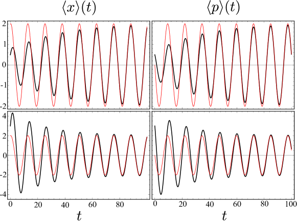
Figure 3: Plot of the average mean values ${\langle{x}\rangle}(t)$ and ${\langle{p}\rangle}(t)$ as a function of time $t$ (black, thick lines) compared to the asymptotic solution given by Eqs. (51) and (52) (red, thin lines). The upper panel corresponds to the initial condition $({\langle{x}\rangle},{\langle{p}\rangle})(0)=(1/2,1/2)$ and the lower one to $({\langle{x}\rangle},{\langle{p}\rangle})(0)=(3,3)$. Other parameters are $\omega=1,\kappa=1/4$ and $y_{0}=2$.

Within the Gaussian assumption, the conditional covariances (i.e., the covariances an observer with access to the measurement result would associate to the state of the system) evolve as for the first scheme according to

$$\frac{d}{dt}V_{x,c} =-\kappa V_{x,c}+2\omega C_{c}-\frac{2\gamma\eta}{\hbar}V_{x,c}^{2}+\kappa\hbar\frac{1+2n_{B}}{2},$$ (53)

$$\frac{d}{dt}V_{p,c} =-\kappa V_{p,c}-2\omega C_{c}-\frac{2\gamma\eta}{\hbar}C_{c}^{2}+\kappa\hbar\frac{1+2n_{B}}{2}+\frac{\hbar\gamma}{2},$$ (54)

$$\frac{d}{dt}C_{c} =\omega(V_{p,c}-V_{x,c})-\kappa C_{c}-\frac{2\gamma\eta}{\hbar}V_{x,c}C_{c}.$$ (55)

In contrast, the unconditional covariances (which an observer without access to the measurement results would associate to the state of the system) obey

$$\frac{d}{dt}V_{x} =(2k-\kappa)V_{x}+2\omega C+\kappa\hbar\frac{1+2n_{B}}{2}+\frac{\hbar k^{2}}{2\gamma\eta},$$ (56)

$$\frac{d}{dt}V_{p} =-\kappa V_{p}-2\omega C+\kappa\hbar\frac{1+2n_{B}}{2}+\frac{\hbar\gamma}{2},$$ (57)

$$\frac{d}{dt}C =\omega(V_{p}-V_{x})+(k-\kappa)C.$$ (58)

Comparing both sets of equations, the most striking difference is that Eqs. (53) – (55) are nonlinear differential equations whereas Eqs. (56) – (58) are linear. Especially note the term proportional to $-\frac{2\gamma\eta}{\hbar}V_{x,c}^{2}$ in Eq. (53), which tends to squeeze the wavepacket in the $x$-direction. This is the effect of the continuous measurement performed on the system, which tends to localize the state. However, if we average over (or, equivalently, ignore) the measurement results, this effect is missing. Furthermore, note that Eqs. (53) – (55) do not contain the parameter $k$, which quantifies how strongly we feed back the signal.

Solving Eqs. (53) – (55) for its steady state is possible, but the exact expressions are extremely lengthy. However, to see how the continuous measurement influences the conditional covariances we will have a look at the special case of no damping ($\kappa=0$). To appreciate this case we remind us that the steady state covariances of a damped HO for no measurement and no feedback are given by $V_{x}=V_{p}=\hbar(n_{B}+\frac{1}{2})$ and $C=0$. Especially, at zero temperature ($n_{B}=0$), we have a minimum uncertainty wave packet satisfying the lower bound of the Heisenberg uncertainty relation, $V_{x}V_{p}=\hbar^{2}/4$. Now, for $\kappa=0$, we can expand the conditional covariances in powers of $\gamma$:

$$\lim_{t\rightarrow\infty}V_{x,c}(t) =\frac{\hbar}{2\sqrt{\eta}}-\frac{\sqrt{\eta}\hbar\gamma^{2}}{16\omega^{2}}+{\cal{O}}(\gamma^{3}),$$ (59)

$$\lim_{t\rightarrow\infty}V_{p,c}(t) =\frac{\hbar}{2\sqrt{\eta}}+\frac{3\sqrt{\eta}\hbar\gamma^{2}}{16\omega^{2}}+{\cal{O}}(\gamma^{3}),$$ (60)

$$\lim_{t\rightarrow\infty}C_{c}(t) =\frac{\hbar\gamma}{4\omega}+{\cal{O}}(\gamma^{3}).$$ (61)

We see that the uncertainty in position is reduced at the expense of an increased uncertainty in momentum. This is exactly what we have to expect from a position measurement due to Heisenberg’s uncertainty principle. Note that this effect is weakened for larger frequencies $\omega$ of the oscillator, because the continuous measurement has problems to “follow” the state appropriately. Furthermore, an imperfect detector ($\eta<1$) will always increase the variances. Finally, we remark that these results become meaningless in the strict limit $\gamma\rightarrow 0$, because in that case there is simply no conditional dynamics. This becomes also clear by looking at Eq. (56), in which the last term diverges in this limit, because we would feed back an infinitely noisy signal.

Thus, an observer with access to the measurement record would associate very different covariances to the system in comparison to an observer without that knowledge. However, a detailed discussion of the time evolution of the covariances is beyond the scope of the present paper. Instead, we find it more interesting to discuss the relationship between the present quantum feedback scheme and its classical counterpart, to which we turn now.

5 Classical limit

To take the classical limit in our case we have to use a little trick, because simply taking $\hbar\rightarrow 0$ does not yield the correct result. In fact, for $\hbar\rightarrow 0$ we have from Eq. (8) that $I(t)=\langle x\rangle_{c}(t)$, which only makes sense if we can observe the particle with infinite accuracy, i.e., its conditional probability distribution is a delta function with respect to the position $x$. We explicitly wish, however, to model a noisy classical measurement. We thus additionally demand that $\eta\rightarrow 0$. More specifically, we set $\eta\equiv\hbar/\sigma$ with $\sigma$ finite such that Eq. (8) becomes

$$dI(t)=\langle x\rangle_{c}(t)dt+\sqrt{\frac{\sigma}{2\gamma}}dW(t)$$ (62)

and we remark that the case $\sigma\rightarrow 0$ corresponds to an error-free measurement.

The FPE (22) for the free evolution of the HO with drift vector and diffusion matrix from Eq. (23) becomes for $\hbar\rightarrow 0$ (note that the Bose-Einstein distribution $n_{B}$ contains $\hbar$ as well and needs to be expanded)

$$\begin{split}\frac{\partial}{\partial t}P(x,p,t)&\equiv{\cal{L}}_{0}^{\text{cl}}P(x,p,t)\\ &=\left\{-\nabla^{T}\cdot\binom{\omega p-\frac{\kappa}{2}x}{-\omega x-\frac{\kappa}{2}x}+\frac{\kappa}{2\beta\omega}\nabla^{T}\cdot\nabla\right\}P(x,p,t).\end{split}$$ (63)

To emphasize the fact that the Wigner function $W(x,p)$ becomes an ordinary probability distribution in the classical limit, we denoted it by $P(x,p)$. As expected, we see that Eq. (63) corresponds to a FPE for a Brownian particle in a harmonic potential where position and momentum are both damped (usually one considers only the momentum to be damped RiskenBook1984 ). This peculiarity is a consequence of an approximation made in deriving the ME (1), which is known as the secular or rotating-wave approximation. Nevertheless, one easily confirms that the canonical equilibrium state $P_{\text{eq}}\sim\exp[-\beta\omega(p^{2}+x^{2})/2]$ is a steady state of this FPE as it must be.

Next, it turns out to be interesting to discuss the classical limit of the SME (13) describing the free evolution plus the influence of the continuous noisy measurement. Using Eq. (24) we obtain an equation for the conditional probability distribution $P_{c}(x,p)$

$$P_{c}(x,p,t+dt)=\left\{1+{\cal{L}}_{0}^{\text{cl}}dt+\sqrt{\frac{2\gamma}{\sigma}}(x-\langle x\rangle_{c})dW(t)\right\}P_{c}(x,p,t).$$ (64)

This is a stochastic FPE, which is nonlinear in $P_{c}$. It describes how our state of knowledge changes if we take into account the measurement record (62). However, averaging Eq. (64) over all measurement results yields Eq. (63), which reflects the fact that a classical measurement does not perturb the system. This is in contrast to the quantum case where the average evolution is still influenced by ${\cal{L}}_{\text{meas}}$, see Eq. (6). Hence, the term ${\cal{L}}_{\text{meas}}$ in Eq. (6) is purely of quantum orgin and it describes the effect of decoherence on a quantum state under the influence of a measurement. This effect is absent in a classical world. Exactly the same equation and the same conclusions were already derived by Milburn following a different route MilburnQSO1996 .

The impact of these conclusions is, however, much more severe if one additionally considers feedback. As we will now show, applying feedback based on the use of the stochastic FPE (64), does indeed yield observable consequences even on average. Please note that trying to model the present situation by a classical Langevin equation is nonsensical. If we would use a Langevin equation to describe our state of knowlegde about the system, we would implicitly ascribe an objective reality to the fact that there is a definite position $x_{0}$ and momentum $p_{0}$ of the particle corresponding to a probability distribution $\delta(x-x_{0})\delta(p-p_{0})$. This is, however, not true from the point of view of the observer who has to apply feedback control based on incomplete information (i.e., the noisy measurement record). Results we would obtain from a Langevin equation treatment can only be recovered in the limit of an error-free measurement, i.e., for $\sigma\rightarrow 0$, as we will demonstrate in appendix 7.

For simplicity we will only have a look at the second feedback scheme from Sec. 4, because we can directly obtain the classical limit for the average evolution from Eq. (43). The same situation is, however, also encountered by considering the first scheme. Taking $\hbar\rightarrow 0$ in Eq. (43) together with the coefficients (LABEL:eq_coeff_W_scheme_2) then yields the FPE

$$\frac{\partial}{\partial t}P(x,p,t)=\left\{{\cal{L}}_{0}^{\text{cl}}-\partial_{x}k[x-x^{*}(t)]+\frac{k^{2}\sigma}{2\gamma}\partial_{x}^{2}\right\}P(x,p,t).$$ (65)

The first term to the correction of ${\cal{L}}_{0}^{\text{cl}}$ is the term one would expect for a noiseless feedback loop, too. The second, however, only arises due to the noisy measurement (we see that it vanishes for $\sigma\rightarrow 0$) and causes an additional diffusion in the $x$ direction simply due to the fact that the observer applies a slightly wrong feedback control compared to the “perfect” situation without measurement errors.

We thus conclude this section by noting that the treatment of continuous noisy classical measurements faces similar challenges as in the quantum setting. On average the measurement itself does not influence the classical dynamics, but we see that we obtain new terms even on average if we use this measurement to perform feedback control. Most importantly, because a feedback loop has to be implemented by the observer who has access to the measurement record, it is in general not possible to model this situation with a Langevin equation. Furthermore, we remark that the situation is expected to be even more complicated for time-delayed feedback, where no average description is a priori possible.

6 Summary and outlook

Because we discussed the meaning of our results already during the main text in detail, we will only give a short summary together with a discussion on possible extensions and applications.

We have used two simple feedback schemes, which are known to change the stability of a steady state obtained from linearizing a dynamical system around that fixed point in the classical case. For the simple situation of a damped quantum HO we have seen that on average we obtain the same dynamics for the mean values as expected from a classical treatment and thus, classical control strategies might turn out to be very useful in the quantum realm, too.

However, the fact that a classical control scheme works so well in the quantum regime depends on two crucial assumptions. First of all, we have used a linear system (the HO). Having a non-linear system Hamiltonian (e.g., a Hamiltonian with a quartic potential $\sim\hat{x}^{4}$) would complicate the treatment, because already the equations for the mean values would contain higher order moments, as e.g. ${\langle{x^{3}}\rangle}$ in case of the quartic oscillator. Simply factorizing them as ${\langle{x^{3}}\rangle}\approx{\langle{x}\rangle}^{3}$ would imply that we are already using a classical approximation. However, as in the classical treatment, where the equations of motion are obtained from linearizing a (potentially non-linear) dynamical system around the fixed point, it might also be possible in the quantum regime to neglect non-linear terms in the vicinity of the fixed point. Whether or not this is possible crucially depends on the localization of the state in phase space, i.e., on its covariances. Here, continuous quantum measurements can actually turn out to be helpful, because they tend to localize the wavefunction and counteract a possible spreading of the state.

The second important assumption we used was that we restricted ourselves to continuous variable quantum systems. The reason why we obtained simple equations of motion is related to the commutation relation $[\hat{x},\hat{p}]=i\hbar$, which we implicitly used to obtain the evolution equation for the Wigner function. Formally, phase space methods are also possible for other quantum systems, but the maps are much more complicated CarmichaelBook1999a . For such systems the methods presented here might be useful under certain special assumptions, but in general one should expect them to fail.

7 Appendix

We want to show that the stochastic FPE, which in general describes the incomplete state of knowledge of an observer, reduces to a Langevin equation in the error-free limit, i.e., in the limit in which we have indeed complete knowledge about the state of the system. Because we are only interested in a proof of principle here, we will consider the simplified situation of an overdamped particle. The Langevin equation of an overdamped Brownian particle in an external potential $U(x)$ is usually given as (see, e.g., RiskenBook1984 )

$$\dot{x}(t)=-\frac{2}{\kappa}U^{\prime}(x)+\sqrt{\frac{T}{\kappa}}\xi(t)$$ (66)

with $U^{\prime}(x)\equiv\frac{\partial U(x)}{\partial x}$ and the Gaussian white noise $\xi(t)\equiv\frac{dW(t)}{dt}$. Furthermore, note that our friction constant is $\frac{\kappa}{2}$ and not – as it is often denoted – $\gamma$, because we use $\gamma$ already for the measurement rate. Now, it is important to remark that at this point Eq. (66) simply describes a convenient numerical tool to simulate a stochastic process. By the mathematical rules of stochastic calculus it is guaranteed that the Langevin equation gives the same averages as the corresponding FPE, i.e., the ensemble average $\mathbb{E}[f(x)]$ over all noisy trajectories for some function $f(x)$ is equal to the expectation value $\langle f(x)\rangle$ taken with respect to the solution of the FPE.

In Sec. 5 we have suggested that the correct state of the system based on a noisy position measurement is given by the stochastic FPE (64), which for an overdamped particle becomes (see also Ref. MilburnQSO1996 )

$$P_{c}(x,t+dt)=\left\{1+{\cal{L}}_{0}^{\text{cl}}dt+\sqrt{\frac{2\gamma}{\sigma}}(x-\langle x\rangle_{c})dW(t)\right\}P_{c}(x,t)$$ (67)

with RiskenBook1984

$${\cal{L}}_{0}^{\text{cl}}=\frac{\partial}{\partial x}\left(\frac{2U^{\prime}(x)}{\kappa}+\frac{\partial}{\partial x}\frac{2T}{\kappa}\right).$$ (68)

Furthermore, we have also claimed that the parameter $\sigma$ in (62) quantifies the error of the measurement. This suggests that we should be able to recover the Langevin Eq. (66) in the limit $\sigma\rightarrow 0$ in which we can observe the particle with infinite precision.

To show this we compute the expectation value of the position according to Eq. (67):

$$d{\langle{x}\rangle}_{c}(t)=-\frac{2}{\kappa}{\langle{U^{\prime}(x)}\rangle}_{c}dt+\sqrt{\frac{2\gamma}{\sigma}}V_{c}(t)dW(t)$$ (69)

where $V_{c}={\langle{x^{2}}\rangle}_{c}-{\langle{x}\rangle}_{c}^{2}$ denotes the variance of the particles position. Because the conditional variance enters this equation, we compute its time evolution, too:

$$\begin{split}dV_{c}=&-\frac{4}{\kappa}\left[{\langle{xU^{\prime}(x)}\rangle}_{c}(t)-{\langle{x}\rangle}_{c}(t){\langle{U^{\prime}(x)}\rangle}_{c}(t)\right]dt+\frac{4T}{\kappa}dt-\frac{2\gamma}{\sigma}V_{c}^{2}dt\\ &+\sqrt{\frac{2\gamma}{\sigma}}\left\langle[x-{\langle{x}\rangle}_{c}(t)]^{3}\right\rangle dW(t).\end{split}$$ (70)

To make analytical progress we now need two assumptions. First, we will assume that $P_{c}(x,t)$ is a Gaussian probability distribution. In fact, because the measurement tends to localize the probability distribution and it is itself modeled as a Gaussian process, this assumption seems reasonable. In addition, we expect $P_{c}(x,t)$ to become a delta-distribution in the limit $\sigma\rightarrow 0$, which is a Gaussian distribution, too. This assumption allows us to drop the stochastic term in Eq. (70). Second, within the variance of $P_{c}(x,t)$ we assume that we can expand $U(x)$ in a Taylor series and approximate it by a quadratic function $ax^{2}+bx+c$. This implies ${\langle{xU^{\prime}(x)}\rangle}_{c}(t)\approx a{\langle{x^{2}}\rangle}_{c}(t)+b{\langle{x}\rangle}_{c}(t)$. In fact, this assumption seems also reasonable, because we expect the measurement to be precise enough such that we can locally resolve the evolution of the particle sufficiently well (especially for small $\sigma$); or to put it differently: a measurement only makes sense if the conditional variance $V_{c}$ of $P_{c}(x,t)$ is small enough. Using this approximation, too, we can then write Eq. (70) as

$$\frac{d}{dt}V_{c}(t)=\frac{4\kappa}{2}-\frac{4a}{\kappa}V_{c}-\frac{2\gamma}{\sigma}V_{c}^{2}.$$ (71)

The only physical steady state solution of this equation is

$$\lim_{t\rightarrow\infty}V_{c}(t)=\frac{a\sigma}{\gamma\kappa}\left(\sqrt{1+\frac{2T\gamma\kappa}{a^{2}\sigma}}-1\right).$$ (72)

Inserting this into Eq. (69) yields

$$d{\langle{x}\rangle}_{c}(t)=-\frac{2}{\kappa}{\langle{U^{\prime}(x)}\rangle}_{c}dt+\frac{a}{\kappa}\sqrt{\frac{2\sigma}{\gamma}}\left(\sqrt{1+\frac{2T\gamma\kappa}{a^{2}\sigma}}-1\right)dW(t).$$ (73)

In this equation we can take the limit $\sigma\rightarrow 0$ such that

$$d{\langle{x}\rangle}^{0}_{c}(t)=-\frac{2}{\kappa}{\langle{U^{\prime}(x)}\rangle}^{0}_{c}dt+\sqrt{\frac{4T}{\kappa}}dW(t),$$ (74)

where we introduced a superscript $0$ on all expectation values to denote the error-free limit. This equation looks already very similar to the LE (66). In fact, mathematically this is the LE since from Eq. (62) we can see that the measurement result becomes for $\sigma\rightarrow 0$ $dI(t)={\langle{x}\rangle}_{c}^{0}(t)dt$. This implies that the measurement result is deterministic and not stochastic anymore, which is only compatible if the associated probability distribution $P_{c}(x,t)$ is a delta distribution $\delta(x-x^{*})$ where $x^{*}$ describes the true instantaneous position of the particle without any uncertainty. Then, Eq. (69) becomes

$$dx^{*}(t)=-\frac{2}{\kappa}U^{\prime}(x^{*})dt+\sqrt{\frac{4T}{\kappa}}dW(t).$$ (75)

Now, this equation is not just a numerical tool, but describes real physical objectivity, because $x^{*}$ coincides with the observed position in the lab. This distinction might seem very nitpicking, but it is of crucial importance if we want to perform feedback based on incomplete information.

References

- (1) M.O. Scully, M.S. Zubairy, Quantum Optics (Cambridge University Press, Cambridge, 1997)
- (2) S.L. Braunstein, P. van Loock, Rev. Mod. Phys. 77, 513 (2005)
- (3) C. Weedbrook, S. Pirandola, R. García-Patrón, N.J. Cerf, T.C. Ralph, J.H. Shapiro, S. Lloyd, Rev. Mod. Phys. 84, 621 (2012)
- (4) M. Aspelmeyer, T.J. Kippenberg, F. Marquardt, Rev. Mod. Phys. 86, 1391 (2014)
- (5) L.D. Faddeev, O.A. Yakubovskii, Lectures on quantum mechanics for mathematics students (Student mathematical library vol. 47, American Mathematical Soc., 2009)
- (6) H.M. Wiseman, G.J. Milburn, Quantum Measurement and Control (Cambridge University Press, Cambridge, 2010)
- (7) W.P. Smith, J.E. Reiner, L.A. Orozco, S. Kuhr, H.M. Wiseman, Phys. Rev. Lett. 89, 133601 (2002)
- (8) P. Bushev, D. Rotter, A. Wilson, F. Dubin, C. Becher, J. Eschner, R. Blatt, V. Steixner, P. Rabl, P. Zoller, Phys. Rev. Lett. 96, 043003 (2006)
- (9) G.G. Gillett, R.B. Dalton, B.P. Lanyon, M.P. Almeida, M. Barbieri, G.J. Pryde, J.L. O’Brien, K.J. Resch, S.D. Bartlett, A.G. White, Phys. Rev. Lett. 104, 080503 (2010)
- (10) C. Sayrin, I. Dotsenko, X. Zhou, B. Peaudecerf, T. Rybarczyk, S. Gleyzes, P. Rouchon, M. Mirrahimi, H. Amini, M. Brune, J.M. Raimond, S. Haroche, Nature (London) 477, 73 (2011)
- (11) R. Vijay, C. Macklin, D.H. Slichter, S.J. Weber, K.W. Murch, R. Naik, A.N. Korotkov, I. Siddiqi, Nature (London) 490, 77 (2012)
- (12) D. Riste, C.C. Bultink, K.W. Lehnert, L. DiCarlo, Phys. Rev. Lett. 109, 240502 (2012)
- (13) H.J. Carmichael, An Open Systems Approach to Quantum Optics (Lecture Notes, Springer, Berlin, 1993)
- (14) G. Lindblad, Commun. Math. Phys. 48, 119 (1976)
- (15) V. Gorini, A. Kossakowski, E.C.G. Sudarshan, J. Math. Phys. 17, 821 (1976)
- (16) K. Jacobs, D.A. Steck, Contemp. Phys. 47, 279 (2006)
- (17) A. Barchielli, L. Lanz, G.M. Prosperi, Nuovo Cimento B 72, 79 (1982)
- (18) A. Barchielli, L. Lanz, G.M. Prosperi, Found. Phys. 13, 779 (1983)
- (19) C.M. Caves, G.J. Milburn, Phys. Rev. A 36, 5543 (1987)
- (20) H.M. Wiseman, G.J. Milburn, Phys. Rev. A 47, 642 (1993)
- (21) A.C. Doherty, K. Jacobs, Phys. Rev. A 60, 2700 (1999)
- (22) C. Gardiner, P. Zoller, Quantum Noise (Springer-Verlag, Berlin Heidelberg, 2004)
- (23) H.M. Wiseman, G.J. Milburn, Phys. Rev. Lett. 70, 548 (1993)
- (24) H.M. Wiseman, G.J. Milburn, Phys. Rev. A 49, 1350 (1994)
- (25) H.M. Wiseman, Phys. Rev. A 49, 2133 (1994)
- (26) M. Hillery, R.F. O’Connell, M.O. Scully, E. Wigner, Phys. Rep. 106, 121 (1984)
- (27) H.J. Carmichael, Statistical Methods in Quantum Optics 1: Master Equations and Fokker-Planck Equations (Springer-Verlag, New York, 1999)
- (28) C. Zachos, D. Fairlie, T. Curtright (eds.). Quantum mechanics in phase space: an overview with selected papers (World Scientific, Vol. 34, 2005)
- (29) H. Risken, The Fokker-Planck Equation: Methods of Solution and Applications (Springer-Verlag, Berlin Heidelberg, 1984)
- (30) P. Hövel, E. Schöll, Phys. Rev. E 72, 046203 (2005)
- (31) E. Arthurs, J.L. Kelly, Bell System Tech. J. 44, 725 (1965)
- (32) A.J. Scott, G.J. Milburn, Phys. Rev. A 63, 042101 (2001)
- (33) K. Pyragas, Phys. Lett. A 170, 421 (1992)
- (34) E. Schöll, H.G. Schuster (eds.). Handbook of Chaos Control (Wiley-VCH, Weinheim, 2007)
- (35) V. Flunkert, I. Fischer, E. Schöll (eds.). Dynamics, control and information in delay-coupled systems: an overview (Phil. Trans. R. Soc. A, 371, 1999, 2013)
- (36) S.J. Whalen, M.J. Collett, A.S. Parkins, H.J. Carmichael, Quantum Electronics Conference & Lasers and Electro-Optics (CLEO/IQEC/PACIFIC RIM), IEEE pp. 1756–1757 (2011)
- (37) A. Carmele, J. Kabuss, F. Schulze, S. Reitzenstein, A. Knorr, Phys. Rev. Lett. 110, 013601 (2013)
- (38) F. Schulze, B. Lingnau, S.M. Hein, A. Carmele, E. Schöll, K. Lüdge, A. Knorr, Phys. Rev. A 89, 041801(R) (2014)
- (39) S.M. Hein, F. Schulze, A. Carmele, A. Knorr, Phys. Rev. Lett. 113, 027401 (2014)
- (40) A.L. Grimsmo, A.S. Parkins, B.S. Skagerstam, New J. Phys. 16, 065004 (2014)
- (41) W. Kopylov, C. Emary, E. Schöll, T. Brandes, New J. Phys. 17, 013040 (2015)
- (42) A.L. Grimsmo, arXiv: 1502.06959
- (43) J. Kabuss, D.O. Krimer, S. Rotter, K. Stannigel, A. Knorr, A. Carmele, arXiv: 1503.05722
- (44) W.H. Zurek, S. Habib, J.P. Paz, Phys. Rev. Lett. 70, 1187 (1993)
- (45) G.J. Milburn, Quantum Semiclass. Opt. 8, 269 (1996)