Modeling asymptotically independent spatial extremes based on Laplace random fields

Abstract

We tackle the modeling of threshold exceedances in asymptotically independent stochastic processes by constructions based on Laplace random fields. Defined as mixtures of Gaussian random fields with an exponential variable embedded for the variance, these processes possess useful asymptotic properties while remaining statistically convenient. Univariate Laplace distribution tails are part of the limiting generalized Pareto distributions for threshold exceedances. After normalizing marginal distributions in data, a standard Laplace field can be used to capture spatial dependence among extremes. Asymptotic properties of Laplace fields are explored and compared to the classical framework of asymptotic dependence. Multivariate joint tail decay rates are slower than for Gaussian fields with the same covariance structure; hence they provide more conservative estimates of very extreme joint risks while maintaining asymptotic independence. Statistical inference is illustrated on extreme wind gusts in the Netherlands where a comparison to the Gaussian dependence model shows a better goodness-of-fit. In this application we fit the well-adapted Weibull distribution, closely related to the Laplace distribution, as univariate tail model.

Keywords: spatial extremes; threshold exceedances; asymptotic independence; elliptical distribution; joint tail decay; wind speed.

1 Introduction

Extreme value analysis provides a toolbox for modeling and estimating extreme events in univariate, multivariate, spatial and spatiotemporal processes (Coles, 2001; Beirlant et al., 2004; Davison et al., 2012). Principal objectives of spatial extreme value analysis are the spatial prediction of extremes and the extrapolation of return levels and periods beyond the historically observed range of data. A major distinction of dependence types can be made between asymptotic dependence when $\lim_{u\uparrow 1}\mathrm{pr}(F_{X_{2}}(X_{2})\geq u\mid F_{X_{1}}(X_{1})\geq u)>0$ for two random variables $X_{1}\sim F_{X_{1}}$ and $X_{2}\sim F_{X_{2}}$ and asymptotic independence when the limit is $0$, provided the limit exists. Asymptotic independence can arise in environmental and climatic data for space lags or time lags when the most extreme events become more and more isolated in time, space or space-time. For many processes like wind gust speed or heavy rainfall such behavior seems plausible owing to physical limits, and it is corroborated by empirical findings (Davison et al., 2013; Thibaud et al., 2013; Opitz et al., 2015). In this paper, our objective is to construct asymptotically independent spatial processes that are flexible and tractable models with useful properties for modeling threshold exceedances.

Models for asymptotically independent extremes must adequately capture the joint tail decay rates in multivariate distributions. A first in-depth analysis of joint tail decay was given by Ledford and Tawn (1996, 1997). Closely related bivariate models (Ramos and Ledford, 2009) provide flexibility in the joint tail, yet an explicit definition of the probability density cannot be given when only one component is extreme and the generalization to higher dimensions suffers from the curse of dimensionality. A more flexible characterization of multivariate tail behavior was developed by Wadsworth and Tawn (2013). Useful models pertaining to this framework are obtained by inverting max-stable processes (Wadsworth and Tawn, 2012), allowing for composite likelihood inference. Another approach that spans both asymptotically dependent and asymptotically independent data is presented by Wadsworth et al. (2014), who model bivariate tails by assuming independence among the radial and the angular variable in a pseudo-polar representation.

For lack of a unified theory of asymptotic independence, a variety of modeling approaches have proven useful in practice. They usually suffer from at least one of the following restrictions: joint tail decay rates are difficult to characterize; standard inference methods like classical likelihood are not available; only bivariate models are tractable and useful; the generalization to the infinite-dimensional, spatial setup is not possible; the univariate tail models prescribed by extreme value theory do not directly appear as marginal distributions in the model, necessitating marginal pretransformations that are not natural in the extreme value context.

In the following, we present the novel Laplace model for multivariate and spatial extremes. It provides a good compromise with respect to the aforementioned potential shortcomings. It is parametrized by a covariance function and closely related to standard Gaussian processes based on embedding an exponentially distributed variable for the variance. The resulting univariate distributions are of the Laplace type, and the univariate tails correspond to valid generalized Pareto limits of threshold exceedances. Classical likelihood inference using threshold exceedances is straightforward. Joint tail decay rates and conditional distributions can be characterized in various ways. We use the terminology of spatial processes for simplicity’s sake, but an extension to the spatiotemporal context is possible through spatiotemporal covariance functions. The notion of a multivariate threshold exceedance is not uniquely defined; here we will concentrate on four sensible choices for extreme value analysis: exceedances observed at one fixed site $s$, exceedances of a linear combination of values at $D$ fixed sites, or exceedances of either the maximum or minimum value over $D$ fixed sites.

Section 2 gives a short exposition of some aspects of classical extreme value theory that are necessary to understand univariate tail models, their link to standard Laplace marginal distributions and the notion of asymptotic independence. Section 3 treats definition and inference of the asymptotically independent Laplace model for threshold exceedances, whose tail behavior is characterized and contrasted with the asymptotic dependence case. An application to modeling of spatial wind gust extremes in the Netherlands in Section 4 is followed by the concluding remarks in Section 5.

2 Extreme value theory

Presentations going beyond this short account can be found in Resnick (1987); Beirlant et al. (2004); de Haan and Ferreira (2006).

2.1 Univariate limit distributions

The fundamental limit relation of extreme value theory establishes a three-parameter limit distribution for adequately rescaled maxima of an independent and identically distributed sample $X_{i}$, $i=1,\ldots,n$: if normalizing sequences $a_{n}>0$, $b_{n}$ exist such that

$$\max_{i=1,\ldots,n}a_{n}^{-1}(X_{i}-b_{n})\rightarrow Z,\quad n\rightarrow\infty,$$ (1)

with a nondegenerate random variable $Z$, then the distribution of $Z$ is necessarily of the generalized extreme value type with cdf

$$F_{Z}(z)=\exp\left(-\left[1+\xi{\textstyle{z-\mu\over\sigma}}\right]_{+}^{-1/\xi}\right),$$

with parameters for position $\mu$, for scale $\sigma>0$ and for shape $\xi$. When $\xi=0$, $F_{Z}(z)$ is defined as the corresponding limit $\exp\left(-\exp[-z]\right)\,1(z>0)$. The tail index $\xi$ is crucial to distinguish between Pareto-type (polynomial) decay for $\xi>0$, exponential decay for $\xi=0$ to a finite or infinite essential supremum and inverse polynomial decay to a finite essential supremum for $\xi<0$. By transforming $Z$ to $Z^{*}=0.5\left(1+\xi[Z-\mu]/\sigma\right)^{1/\xi}$, we normalize to a Fréchet distribution $F_{Z^{*}}(z)=\exp(-1/[2z])\,1_{(0,\infty)}(z)$.

Equivalent formulations in terms of threshold exceedances have proven useful both from a conceptual and practical perspective. By absorbing the values of $a_{n}$ and $b_{n}$ into the parameters $\sigma$ and $\mu$, it is then useful to anchor practical modeling in the tail approximation

$$\mathrm{pr}(X\geq x)\approx\left(1+\xi{\textstyle{x-\mu\over\sigma}}\right)^{-1/\xi}=-\log F_{Z}(x),$$ (2)

valid for large $x$. When $\xi=0$, this tail probability is $\mathrm{pr}(X\geq x)\approx\exp(-[x-\mu]/\sigma)$, corresponding to a generalized exponential tail. By conditioning on an exceedance over a high threshold $u$ with $u\geq\mu$ if $\xi\geq 0$ and $u<\mu$ otherwise, we get

$$\mathrm{pr}(X\leq x\mid X\geq u)\approx 1-\left(1+\xi{\textstyle{x-u\over\sigma_{u}}}\right)^{-1/\xi},\quad\sigma_{u}=\sigma+\xi(u-\mu),\quad x\geq u,$$ (3)

where the right-hand side defines the cdf of the limiting generalized Pareto distribution for threshold exceedances $x-u$.

2.2 Normalized marginal distributions

When we treat the dependence structure in a multivariate setting, it is convenient to normalize all univariate marginal distributions to a parameter-free target distribution that appears naturally in the extreme value context. We will focus on standardizations that lead to limit distributions in (1) of the Fréchet type $F_{Z^{*}}(z)=\exp(-1/[2z])$ ($z>0$) with tail index $1$ and scale $0.5$; we call this standardization the $*$-transformation in the following. Here we slightly modify the usual normalization found in the literature (with scale $1$) in order to establish the link to the Laplace distribution more easily in the following. In the literature, we often find $X^{*}=1/[2(1-F_{X}(X))]$, leading to a Pareto target distribution with shape parameter $1$ and lower bound $0.5$ when $F_{X}$ is continuous. Similarly, $X^{*}=-1/[2\log(F_{X}(X))]$ establishes the Fréchet target distribution $F_{X^{*}}(x)=F_{Z^{*}}(x)$ when $F_{X}$ is continuous. It is possible to use more general probability integral transforms for $*$ , as long as they lead to nonnegativity and standard Pareto tail behavior, i.e., $\mathrm{pr}(X^{*}\geq 0)=1$ and $2x\times\mathrm{pr}(X^{*}\geq x)\rightarrow 1$ for $x\rightarrow\infty$.

Concerning the behavior in the bulk of the target distribution, there is no other constraint than nonnegativity since the normalization of $X^{*}$ by $a_{n}=n$ drives all non-extreme values from the bulk to $0$ in the limit. However, when modeling and estimating multivariate or spatial extremal behavior from a finite sample of data, we often also need to specify the bulk behavior in the target distribution, see Coles and Tawn (1991); Wadsworth and Tawn (2012); de Carvalho and Davison (2014), for instance. For a useful choice of target distribution, we here focus on the following two properties: (1) a decreasing density on $(0,\infty)$: $f_{X^{*}}(x_{1})\geq f_{X^{*}}(x_{2})$ for any $0<x_{1}\leq x_{2}<\infty$ (2) exact Pareto tail behavior: $\mathrm{pr}(X^{*}\geq x)=1/(2x)$ for $x\geq u$ with $u>0.5$ chosen as small as possible. These conditions yield a $*$-transformation ensuring a distribution of $X^{*}$ that is as close as possible to the asymptotic univariate limit since the convergence of maxima to $Z^{*}$ is equivalent to the convergence of the renormalized sample $\{X^{*}_{i}/n,\,i=1,\ldots,n\}$ to a Poisson limit process on $[0,\infty)$ with decreasing intensity $\mathrm{d}x/(2x^{2})$ associated to the intensity measure $\Lambda([x,\infty))=1/(2x)$. The only distribution to satisfy these requirements is characterized by the density

$$f_{X^{*}}(x)=\begin{cases}1/(2x^{2})&\text{ if }x\geq 1,\\ 0.5&\text{ if }0\leq x<1,\\ 0&\text{ otherwise. }\end{cases}$$ (4)

This target distribution is a mixture with probability $0.5$ of a uniform distribution on $(0,1)$ and a standard Pareto distribution on $[1,\infty)$. Its importance for the following developments comes from considering the distribution of $\log X^{*}$, whose density defines the standard Laplace distribution (Kotz et al., 2001),

$$f_{\log X^{*}}(x)=0.5\exp(-|x|).$$

Therefore, the Laplace distribution can be considered as a natural standard marginal distribution for the modeling of multivariate extreme values.

2.3 Multivariate and spatial limits

Univariate limits are readily generalized to the multivariate and spatial domain. For a sequence of independent and identically distributed copies $\{X_{i}(s)\}$ ($i=1,2,\ldots,n$) of a spatial process $\bm{X}=\{X(s)\}$, we need normalizing sequences $a_{n}(s)>0$, $b_{n}(s)$ such that the convergence of componentwise maxima holds in terms of finite-dimensional distributions:

$$\max_{i=1,\ldots,n}a_{n}(s)^{-1}(X_{i}(s)-b_{n}(s))\rightarrow Z(s),\quad n\rightarrow\infty,$$ (5)

with nondegenerate marginal distributions in the limiting max-stable process $\bm{Z}=\{Z(s)\}$; we say that $\bm{X}$ is in the maximum domain of attraction of $\bm{Z}$. The univariate convergence of marginal distributions corresponds to the theory in Section 2.1. We say that a vector $X(\bm{s})=(X(s_{1}),\ldots,X(s_{D}))$ is asymptotically independent if the components $Z(s_{j})$, $j=1,\ldots,D$, are mutually independent. The limiting dependence structure of a multivariate vector can be characterized for $*$-transformed margins. Convergence (5) is equivalent to the convergence of all univariate distributions in the sense of (1) together with the following condition: a $(-1)$-homogeneous measure $\eta$ with $\eta(tA)=t^{-1}\eta(A)$ exists such that, for any set $A$ relatively compact in $[\bm{0},\bm{\infty}]\setminus\{\bm{0}\}\subset\overline{\mathbb{R}}^{D}$ with $\eta(\partial A)=0$, we have

$$t\,\mathrm{pr}(X^{*}(\bm{s})/t\in A)\rightarrow\eta(A),\quad t\rightarrow\infty,$$ (6)

for the marginally normalized vector $X^{*}(\bm{s})$. Loosely speaking, the vague convergence property (6) means that we can use the approximation $\mathrm{pr}(X^{*}(\bm{s})\in A)\approx\eta(A)$ for “extreme” sets $A$ bounded far from the origin $\bm{0}$. In practice, the homogeneity of $\eta$ provides a simple formula for the extrapolation of extreme event probabilities to more extreme yet hitherto unobserved events: $\mathrm{pr}(X^{*}(\bm{s})\in tA)\approx t^{-1}\mathrm{pr}(X^{*}(\bm{s})\in A)$, for $t\geq 1$ and an extreme event $A$. By transforming $X^{*}(\bm{s})$ to $\log X^{*}(\bm{s})$, this relation can equivalently be written as $\mathrm{pr}(\log X^{*}(\bm{s})-t\in A)\approx\exp(-t)\,\tilde{\eta}(A)$ with $\tilde{\eta}=\eta\circ\exp$, $t\geq 0$ and $A\subset\mathbb{R}^{D}$ an extreme event. Finally, we point out that $\eta((\bm{0},\bm{\infty}))=0$ when $X(\bm{s})$ is asymptotically independent, i.e., the limit measure $\eta$ has a singular structure with all of its mass concentrated on the Euclidean axes.

2.4 Tail dependence coefficients

Bivariate tail dependence coefficients are useful summaries of tail dependence, and in a spatial context we can study their evolution with respect to the spatial lag between two sites. The tail correlation coefficient $\lambda$ of a bivariate random vector $(X_{1},X_{2})$ is defined as

$$\lambda =\lim_{u\uparrow 1}\mathrm{pr}(F_{X_{2}}(X_{2})\geq u\mid F_{X_{1}}(X_{1})\geq u)$$

$$=\lim_{u\uparrow 1}\mathrm{pr}(F_{X_{2}}(X_{2})\geq u,F_{X_{1}}(X_{1})\geq u)/(1-u)\in[0,1].$$ (7)

It is well-defined and symmetric in $X_{1}$ and $X_{2}$ if $(X_{1},X_{2})$ is in a bivariate maximum domain of attraction. Its value is $0$ if and only if $X_{1}$ and $X_{2}$ are asymptotically independent. If this is the case, more information is provided by the residual coefficient $\rho\in[0,1]$ (Ledford and Tawn, 1996; Draisma et al., 2004), where

$$\mathrm{pr}(X_{1}^{*}\geq x,X_{2}^{*}\geq x)=\ell(x)x^{-1/\rho}$$ (8)

for large $x$ with $\ell(x)>0$ a slowly varying function such that $\ell(tx)/\ell(t)\rightarrow 1$ for $x>0$ and $t\rightarrow\infty$. When $\rho$ is positive, it corresponds to the tail index $\xi$ of $\min(X_{1}^{*},X_{2}^{*})$. For independent variables $X_{1}$ and $X_{2}$, we have $\rho=0.5$. We remark that $\rho$ is always equal to $1$ when $X_{1}$ and $X_{2}$ are asymptotically dependent, such that it is of interest to study either $\lambda$ or $\rho$, depending on the presence of asymptotic dependence. For the bivariate Gaussian distribution, the residual coefficient is $(1+\rho_{\mathrm{lin}})/2$, with $\rho_{\mathrm{lin}}$ the linear correlation coefficient, and covers the full range $[0,1]$ of theoretically possible values when $\rho_{\mathrm{lin}}$ varies from $-1$ to $1$. In the following, we exclude the case $\rho=0$ corresponding to strong negative assocation of $X_{1}$ and $X_{2}$. The residual coefficient $\rho$ can also be defined more generally for $D>2$ by

$$\mathrm{pr}(X_{1}^{*}\geq x,\ldots,X_{D}^{*}\geq x)=\ell(x)x^{-1/\rho}$$ (9)

for large $x$ if an adequately defined slowly varying function $\ell$ exists.

2.5 From modeling to inference of extremal dependence

Since there is no natural ordering of multivariate data, different notions of threshold exceedances can be of interest with respect to the application context but also with respect to tractability of statistical inference. We focus on four useful choices that are common in the literature. Given a fixed threshold $u$, a vector $\bm{x}$ is a marginal exceedance in $x_{1}$ if $x_{1}\geq u$, it is a sum exceedance if $\sum_{j=1}^{D}x_{j}\geq u$, it is a max exceedance if $\max_{j=1,\ldots,D}x_{j}\geq u$, and it is a min exceedance if $\min_{j=1,\ldots,D}x_{j}\geq u$. For the corresponding exceedance sets, we write $A_{x_{1}}(u)=\{\bm{x}\mid x_{1}\geq u\}$, $A_{\mathrm{sum}}(u)=\{\bm{x}\mid\sum_{j}x_{j}\geq u\}$, $A_{\mathrm{max}}(u)=\{\bm{x}\mid\max_{j}x_{j}\geq u\}$ and $A_{\mathrm{min}}(u)=\{\bm{x}\mid\min_{j}x_{j}\geq u\}$. The limit (6) holds for these sets when $u>0$.

Whereas models for asymptotically dependent data have a strong theoretical foundation, there is no natural model class for describing how asymptotically independent data approach their limit. Using the limiting asymptotic independence would usually be too simplistic (by imposing independence among maxima of components, for instance), and it would considerably underestimate joint risks at the subasymptotic level. It is therefore sensible to focus on extremal dependence models that adequately capture the rate of convergence towards asymptotic independence. A simple approach consists in combining an appropriate model for univariate tails with a Gaussian dependence model. Known as Gaussian copula modeling (Davison et al., 2012), this approach has been explored by Bortot et al. (2000) for oceanographic data and by Renard and Lang (2007) for hydrological data, among others. Its extension to the spatial domain is straightforward.

For exploratory analysis, it is useful to investigate estimates of tail dependence coefficients based on the empirical counterparts of (7) and (8). In the spatial context, one can study their variation with distance. For Gaussian copula modeling, likelihood estimators ${\widehat{\rho}}_{\mathrm{lin}}$ of the linear correlation $\rho_{\mathrm{lin}}$, based on threshold exceedances, are readily defined and yield an estimate $(1+{\widehat{\rho}}_{\mathrm{lin}})/2$ of the residual coefficient. Likelihood estimation based on threshold exceedances is a standard approach for both asymptotically dependent and asymptotically independent data. After fixing an exceedance region $A$, we assume a parametric distribution $F_{A}$ according to a parameter vector $\bm{\theta}$ for exceedances $\bm{X}\mid\bm{X}\in A\sim F_{A}$. The choice of threshold $u$ in $A$ is rarely straightforward since it is usually a trade-off between bias and variance. If a lower threshold decreases estimation variance by using more information from data, one also has to take into account the rate of convergence towards the asymptotic regimes used for modeling. The likelihood $L$ for jointly estimating the exceedance probability $\mathrm{pr}(\bm{X}\in A)$ and the extremal behavior is based on the censoring of data $\bm{x}$ not falling into $A$:

$$L(\bm{\theta};\bm{x})=1_{A^{C}}(\bm{x})\times(1-\mathrm{pr}(\bm{X}\in A))+1_{A}(\bm{x})\mathrm{pr}(\bm{X}\in A)f_{A}(\bm{x})$$ (10)

where $f_{A}$ is the density of the exceedance distribution $F_{A}$.

3 Properties and modeling of exceedances of Laplace random fields

3.1 Laplace random fields

We denote $\bm{W}=\{W(s),s\in K\}$ a Gaussian random field defined on a nonempty domain $K$. Multivariate distributions represent a special case by setting $K=\{1,\ldots,D\}$ for $D\in\mathbb{N}$. We provide the constructive definition of Laplace random fields as a mixture of Gaussian fields based on embedding an exponential variable with scale $2$ for the variance of the Gaussian field. This definition and basic properties can be found in the monograph of Kotz et al. (2001). Multivariate Laplace distributions are also discussed in Eltoft et al. (2006).

Definition 1 (Laplace random field).

For $\bm{W}$ a centered Gaussian random field and a random variable $Y\geq 0$ with $Y^{2}$ following an exponential distribution with scale $2$ and independent of $\bm{W}$, the random field

$$\bm{X}=\{X(s),s\in K\}=\{YW(s),s\in K\}$$ (11)

is called Laplace random field (or Laplace field in short). We call $\bm{X}$ a standard Laplace field if $\bm{W}$ is a standard Gaussian field. If $\bm{W}$ has a covariance function or covariance matrix $\Sigma$, we write $\bm{X}\sim\mathcal{L}(\Sigma)$.

The distribution of $Y$ is known as Rayleigh distribution with parameter $1$. For standard Laplace vectors, we use the notation $\Sigma^{*}$ to indicate that $\Sigma^{*}$ is a correlation matrix. In the remainder of this paper, the default assumption is that $\Sigma$ has full rank such that the inverse $\Sigma^{-1}$ is well defined. The univariate marginal distributions $F_{X(s)}$ of a standard Laplace field $\bm{X}$ are symmetric with mean $0$ and variance $2$, and they have pdf $f_{X(s)}(x)=0.5\exp(-|x|)$ corresponding to the univariate Laplace distribution. The variable $Y$ has pdf $f_{Y}(y)=y\exp(-0.5y^{2})$. The covariance function of $\bm{X}$ is $2\Sigma$. If $\Sigma(\bm{s})$ is the covariance matrix of $W(\bm{s})=(W(s_{1}),\ldots,W(s_{D}))$, the conditional distribution of $X(\bm{s})$ given $Y=y$ is Gaussian with covariance $y^{2}\Sigma(\bm{s})$. Using the notation $\nu=0.5(2-D)$, the pdf of $X(\bm{s})$ is

$$f_{X(\bm{s})}(\bm{x})={\textstyle{2^{0.5}\over(2\pi)^{0.5D}|\Sigma(\bm{s})|^{0.5}}}\left(0.25\bm{x}^{\prime}\Sigma(\bm{s})^{-1}\bm{x}\right)^{0.5\nu}K_{\nu}\left(\sqrt{\bm{x}^{\prime}\Sigma(\bm{s})^{-1}\bm{x}}\right).$$ (12)

Here, $K_{\nu}$ is the modified Bessel function of the third kind, see Equation (A.0.4) in Kotz et al. (2001). Whereas marginal densities are continuous but not differentiable at $0$, the joint density $f_{X(\bm{s})}$ has a singularity at $\bm{0}$ for $D>1$ such that $f_{X(\bm{s})}(\bm{x})\rightarrow\infty$ when $\|\bm{x}\|\rightarrow 0$. Since our interest will be directed towards extreme events with $\|\bm{x}\|$ strictly separated from $0$, we can neglect this particularity.

Laplace vectors are part of the larger class of elliptically contoured random vectors, which can be represented using a random radial variable $R\geq 0$ and a $D\times D$ deterministic matrix $A$ that operates on a random vector $\bm{U}$, independent of $R$, with uniform distribution over the Euclidean unit sphere in $\mathbb{R}^{D}$. Then $RA\bm{U}$ defines an elliptic random vector with dispersion matrix $\Sigma=AA^{\prime}$. For the multivariate Laplace distribution, we get (Kotz et al., 2001)

$$f_{R}(r)=2^{1-0.25D}\Gamma(0.5D)^{-1}r^{D-1}K_{0.5D-1}(r),\quad r>0.$$

For Laplace vectors, we get $X(\bm{s})=YW(\bm{s})=YR_{W(\bm{s})}A\bm{U}$ with $R_{W(\bm{s})}$ and $\Sigma(\bm{s})=AA^{\prime}$ associated to the elliptical Gaussian vector $W(\bm{s})$. The dispersion matrices of the Gaussian vector and the Laplace vector are the same and the random vectors differ only by their radial variable.

3.2 Asymptotic behavior of exceedances

The univariate standard Laplace tails with $\mathrm{pr}(X(s)\geq x)=0.5\exp(-x)$ for $x>0$ correspond to the univariate tail model (2) with $\xi=0$, $\sigma=1$ and $\mu=-\log 2$. For exceedances above a fixed threshold $u>0$, we get the conditional generalized Pareto distribution $F_{X(s)\mid X(s)\geq u}(x)=1-\exp(-(x-u))$ for $x\geq u$ according to (3).

We now characterize multivariate tail behavior of a Laplace vector denoted as $\bm{X}=(X_{1},\ldots,X_{D})\sim\mathcal{L}(\Sigma)$ with $\Sigma=(\sigma_{j_{1}j_{2}})_{1\leq j_{1},j_{2}\leq D}$. Due to the elliptical structure of its distribution, weighted sums of the components of $\bm{X}$ are Laplace distributed: $\sum_{j=1}^{D}\omega_{j}X_{j}\sim\mathcal{L}(\bm{\omega}^{\prime}\Sigma\bm{\omega})$, and we have sum-stability with respect to the generalized Pareto tail family with $\xi=0$, $\mu=-\log 2$ and $\sigma_{u}=\sqrt{\bm{\omega}^{\prime}\Sigma\bm{\omega}}$. The mean of the components of $\bm{X}$ follows a $\mathcal{L}(D^{-2}\sum_{1\leq j_{1},j_{2}\leq D}\sigma_{j_{1}j_{2}})$ distribution. When $\Sigma=\Sigma^{*}$, then $\bm{X}^{*}=\exp(\bm{X})$ has standard log-Laplace margins (4) whose shape parameter is $\xi=1$, and the geometric mean of components has tail behavior leading to a Pareto exceedance distribution with shape parameter $\xi=D^{-2}\sum_{1\leq j_{1},j_{2}\leq D}\sigma_{j_{1}j_{2}}\leq 1$ for values above $u=1$. This is in contrast to the multivariate standard Pareto limits for asymptotically dependent distributions, where sums of components are again Pareto distributed with shape $\xi=1$, see Falk and Guillou (2008).

A useful coefficient of tail dependence for Laplace vectors can be defined through the scale parameter $\sigma=(\sum_{1\leq j_{1},j_{2}\leq D}\sigma^{*}_{j_{1}j_{2}})^{0.5}$ of the sum of components, where $\sigma^{*}_{j_{1}j_{2}}$ are the entries of the correlation matrix $\Sigma^{*}$ associated to $\Sigma$ in order to remove the effect of the marginal scale. When $D=2$, this coefficient is $\sqrt{2(1+\sigma^{*}_{12})}$ and varies between $0$ (for $\sigma^{*}_{12}=-1$) and $2$ (for $\sigma^{*}_{12}=1$). When $D>2$, it is lower-bounded by $0$ and reaches its upper bound $D$ in the case of complete dependence ($\sigma^{*}_{j_{1}j_{2}}=1$ for all $1\leq j_{1},j_{2}\leq D)$. This coefficient allows us to see how pairwise coefficients relate to higher-order coefficients, which is not straightforward for the standard coefficients $\lambda$ and $\rho$ of extreme value theory defined in Section 2.4, see Schlather and Tawn (2003) for inequalities related to $\lambda$ in a multivariate context, and see Strokorb et al. (2015) for spatial properties.

Proposition 1 (Joint tail decay rates).

The residual coefficient of $(X_{1},X_{2})\sim\mathcal{L}(\Sigma^{*})$ with $\sigma^{*}_{12}=\rho_{\rm lin}$ is $\rho=\sqrt{(1+\rho_{\rm lin})/2}$. The joint tail decay is characterized by a conditional limit for $x,y\in(0,1]$ when $u\rightarrow\infty$,

$$\mathrm{pr}(X_{1}>q_{1-x/u},X_{2}>q_{1-y/u}\mid X_{1}>q_{1-1/u},X_{2}>q_{1-1/u})\rightarrow(xy)^{1/(2\rho)},$$ (13)

where $q_{p}$ is the quantile of the standard Laplace distribution associated to the probability $p\in(0,1)$. The multivariate residual coefficient defined in (9) is $\rho=1/\sqrt{\bm{e}^{\prime}(\Sigma^{*})^{-1}\bm{e}}$ for a Laplace random vector $\bm{X}\sim\mathcal{L}(\Sigma)$ with $\Sigma^{*}$ the correlation matrix associated to $\Sigma$ and $\bm{e}=(1,\ldots,1)^{\prime}$.

Proof.

For the bivariate results, we check the conditions stated in Theorem 2.1 of Hashorva (2010), which establishes joint tail decay rates for a large class of bivariate elliptical random vectors. The theorem states the following: if a function $w(\cdot)$ and the so-called Weibull tail coefficient $\theta\geq 0$ exist such that

$$\lim_{r\rightarrow\infty}{\textstyle{1-F_{R}(r+t/w(r))\over 1-F_{R}(r)}}=\exp(-t)\ \forall t\in\mathbb{R},\quad\lim_{t\rightarrow\infty}w(ct)/w(t)=c^{\theta-1}\ \forall c>0,$$

then $\rho=([1+\rho_{\rm lin}]/2)^{\theta/2}$. In our case, we exploit that the Bessel function of the third kind has asymptotic behavior $K_{\nu}(x)\sim\sqrt{\pi/(2x)}\exp(-x)$ when $x$ tends to infinity. Therefore, $f_{R}(r)\sim c_{R}\sqrt{r}\exp(-r)$ with a constant $c_{R}>0$. Using l’Hôpital’s rule, we obtain

$$\lim_{r\rightarrow\infty}{\textstyle{1-F_{R}(r+t)\over 1-F_{R}(r)}}=\lim_{r\rightarrow\infty}{\textstyle{\sqrt{r+t}\exp(-(r+t))\over\sqrt{r}\exp(-r)}}=\exp(-t).$$

We have $w(t)=1=t^{\theta-1}$ with $\theta=1$, yielding $\rho=\sqrt{(1+\rho_{\mathrm{lin}})/2}$. The convergence (13) is a special case of Theorem 2.1 from Hashorva (2010), where we exclude the cases $x>1$ or $y>1$ to obtain our slightly simpler formulation in terms of conditional probabilities. The general multivariate residual coefficient is obtained in Example 1 of Nolde (2014) with $\alpha=1$ for the Laplace distribution. ∎

For given linear correlation coefficient $\rho_{\rm lin}$, the bivariate residual coefficient of Laplace distributions is the square root of the Gaussian equivalent. The slower joint tail decay rate is due to the stochastic variance embedded in the Gaussian process. A bivariate Laplace vector with $\rho_{\rm lin}=0$ has uncorrelated components $X_{1}$ and $X_{2}$, but the corresponding residual coefficient $1/\sqrt{2}$ is different from $1/2$ corresponding to independent $X_{1}$ and $X_{2}$. The following proposition resumes the extrapolation of probabilities for exceedance sets.

Proposition 2 (Extrapolation of exceedance probabilities).

For $\bm{X}\sim\mathcal{L}(\Sigma)$ a $D$-dimensional Laplace vector, $u>0$ a threshold and $\bm{t}=(t,\ldots,t)>0$ defining a translation $\bm{X}-\bm{t}$ of the vector, we observe:

$$\mathrm{pr}(\bm{X}-\bm{t}\in A_{\mathrm{sum}}(u)) =\exp\left(-{\textstyle{D\over\sqrt{\bm{e}^{\prime}\Sigma\bm{e}}}}\times t\right)\mathrm{pr}(\bm{X}\in A_{\mathrm{sum}}(u)),$$

$$\mathrm{pr}(\bm{X}-\bm{t}\in A_{x_{1}}(u)) =\exp\left(-t/\sqrt{\sigma_{11}}\right)\mathrm{pr}(\bm{X}\in A_{x_{1}}(u)),$$

$$\mathrm{pr}(\bm{X}-\bm{t}\in A_{\mathrm{max}}(u)) \sim\exp\left(-t/\sigma\right)\mathrm{pr}(\bm{X}\in A_{\mathrm{max}}(u)),\quad u\rightarrow\infty,$$

where $\sigma=\sqrt{\max(\sigma_{11},\ldots,\sigma_{DD})}$ in the last equation. When $\Sigma=\Sigma^{*}$ is a correlation matrix, we further have

$$\mathrm{pr}(\bm{X}-\bm{t}\in A_{\mathrm{min}}(u))\sim\exp\left(-\sqrt{\bm{e}^{\prime}(\Sigma^{*})^{-1}\bm{e}}\times t\right)\mathrm{pr}(\bm{X}\in A_{\mathrm{min}}(u)),\quad u\rightarrow\infty.$$

Proof.

The exact tail decay rate for sum exceedances follows directly from the sum stability of the Laplace distribution, here with $\bm{\omega}=\bm{e}$:

$$\mathrm{pr}(\bm{X}-\bm{t}\in A_{\mathrm{sum}}(u)) =\mathrm{pr}\left(\sum_{j=1}^{D}X_{j}\geq Dt+u\right)$$

$$=0.5\exp\left(-(Dt+u)/\sqrt{\bm{e}^{\prime}\Sigma\bm{e}}\right)$$

$$=\exp\left(-Dt/\sqrt{\bm{e}^{\prime}\Sigma\bm{e}}\right)\times\mathrm{pr}(\bm{X}\in A_{\mathrm{sum}}(u)).$$

Similarly, the exact rate of marginal exceedances is obtained by setting $\bm{\omega}=(1,0,\ldots,0)$. To derive the formula for maxima, we first consider the case where $\sqrt{\sigma_{jj}}=\sigma>0$ is constant for $j=1,\ldots,D$. Then $\bm{X}^{*}=\exp(\bm{X}/\sigma)$ is of standard log-Laplace type with density (4) and satisfies the convergence (6). By defining $t^{*}=\exp(t/\sigma)$ and $u^{*}=\exp(u/\sigma)$, we find that both of the expressions $u^{*}\,\mathrm{pr}(\bm{X}^{*}\in A_{\max}(u^{*}))$ and $t^{*}u^{*}\,\mathrm{pr}(\bm{X}^{*}\in A_{\max}(t^{*}u^{*}))$ tend to $\eta(A_{\max}(1))=D$ as $u^{*}\rightarrow\infty$, where $\eta(A_{\max}(1))$ is the extremal coefficient whose value is $D$ under asymptotic independence. Since $D>0$, we get $\mathrm{pr}(\bm{X}^{*}\in A_{\max}(t^{*}u^{*}))\sim(t^{*})^{-1}\mathrm{pr}(\bm{X}^{*}\in A_{\max}(u^{*}))$. In terms of $\bm{X}$, $t$ and $u$, we get the stated convergence rate $\mathrm{pr}(\bm{X}-\bm{t}\in A_{\mathrm{max}}(u))\sim\exp\left(-t/\sigma\right)\mathrm{pr}(\bm{X}\in A_{\mathrm{max}}(u))$. In the case where the diagonal values of $\Sigma$ are not constant such that $\sigma_{j_{0}j_{0}}=\max_{j=1,\ldots,D}\sigma_{jj}$ for $j_{0}\in J$ with $1\leq|J|<D$, we start by observing that

$$\mathrm{pr}\left(\max_{j_{0}\in J}X_{j_{0}}\geq u\right)\leq\mathrm{pr}\left(\bm{X}\in A_{\max}(u)\right)\leq\mathrm{pr}\left(\max_{j_{0}\in J}X_{j_{0}}\geq u\right)+\sum_{j\not\in J}\mathrm{pr}(X_{j}\geq u).$$ (14)

Since $0\leq\mathrm{pr}(X_{j}\geq u)/\mathrm{pr}(\max_{j_{0}\in J}X_{j_{0}}\geq u)\leq\mathrm{pr}(X_{j}\geq u)/\mathrm{pr}(X_{j_{1}}\geq u)\rightarrow 0$ as $u\rightarrow\infty$ for any $j_{1}\in J$ and $j\not\in J$, dividing the inequality (14) by $\mathrm{pr}(\max_{j_{0}\in J}X_{j_{0}}\geq u)$ shows that $\mathrm{pr}(\bm{X}\in A_{\max}(u))\sim\mathrm{pr}(\max_{j_{0}\in J}X_{j_{0}}\geq u)$ when $u\rightarrow\infty$, and the convergence rate of maxima of $\bm{X}$ is the same as the convergence rate of maxima of the subvector $\bm{X}_{J}$. Applying the result for constant diagonal elements $\sigma_{j_{0}j_{0}}$, $j_{0}\in J$ to $\bm{X}_{J}$ then proves the statement for maxima. The asymptotic rate for min exceedances is directly linked to the definition of the multivariate residual coefficient $\rho$ whose value is given in Proposition 1. ∎

When $\Sigma=\Sigma^{*}$ such that margins of $\bm{X}$ are standard Laplace, then (6) holds for $\bm{X}^{*}=\exp(\bm{X})$ and the limit measure $\eta$ is zero for the sets $\exp(A_{\rm sum}(u))$ and $\exp(A_{\rm min}(u))$ that lie within $(\bm{0},\bm{\infty})$. The decay rates are faster for these exceedance types than for $A_{x_{1}}$ and $A_{\rm max}$ where decay rates are determined by the univariate marginal decay rate. Proposition 2 shows that $t\,\mathrm{pr}(\bm{X}^{*}/\tilde{t}\in A)$ tends to a finite positive limit when choosing $\tilde{t}=t^{\sqrt{\bm{e}^{\prime}\Sigma^{*}\bm{e}}/D}$ for $A_{\mathrm{sum}}$ and $\tilde{t}=t^{1/\sqrt{\bm{e}^{\prime}(\Sigma^{*})^{-1}\bm{e}}}$ for $A_{\mathrm{min}}$.

The sum stability of elliptical distributions further provides exact formulas for related exceedance probabilities: $\mathrm{pr}(\bm{X}\in A_{\mathrm{sum}}(u))=0.5\exp(-u/\sqrt{\bm{e}^{\prime}\Sigma\bm{e}})$ and $A_{x_{1}}(u)=0.5\exp(-u/\sqrt{\sigma_{11}})$. To avoid plain Monte-Carlo approaches for calculating probabilities $\mathrm{pr}(\bm{X}\not\leq\bm{x})=\mathrm{pr}(X_{j}>x_{j}\text{ for at least one }j)$ which can be too inaccurate or too slow in certain cases, we can instead exploit tailor-made algorithms for calculating multivariate normal probabilities $\Phi_{\Sigma}(\bm{x})$ (Genz and Bretz, 2009). Univariate numerical integration then yields more accurate values based on

$$\mathrm{pr}(\bm{X}\not\leq\bm{x})=1-\int_{0}^{\infty}\Phi_{\Sigma}(\bm{x}/y)f_{Y}(y)\,\mathrm{d}y.$$ (15)

3.3 Conditional distributions

The following proposition provides a basis for conditional simulation of Laplace random vectors conditional to the value of a subvector. When $\bm{X}=(\bm{X}_{1},\bm{X}_{2})\sim\mathcal{L}(\Sigma)$ is a $D$-dimensional Laplace vector with $\bm{X}_{1}=(X_{1},\ldots,X_{d})$ for $d\in\{1,\ldots,D-1\}$, we write $\Sigma_{ij}$, $1\leq i,j\leq 2$ for the corresponding blocks of the dispersion matrix $\Sigma$.

Proposition 3 (Conditional distributions).

1. When $\bm{X}=Y\bm{W}\sim\mathcal{L}(\Sigma)$ with mixing variable $Y\geq 0$, $Y^{2}\sim\mathrm{Exp}$ with scale $2$, conditioning on $\bm{X}=\bm{x}$ yields the conditional density of $Y$ given as

   $$f_{Y\mid\bm{X}=\bm{x}}(y)=c(\bm{x},\Sigma)\times y^{-(D-1)}\exp\left(-0.5[y^{2}+\bm{x}^{\prime}\Sigma^{-1}\bm{x}/y^{2}]\right),$$

   with the constant $c(\bm{x},\Sigma)=(2\pi)^{-0.5D}|\Sigma|^{-0.5}/f_{\bm{X}}(\bm{x})>0$ depending only on $\bm{x}$ and $\Sigma$. For $D=1$ and $\Sigma=(1)$, we obtain the conditional density

   $$f_{Y\mid X=x}(y)=2^{0.5}\pi^{-0.5}\exp\left(-0.5[y^{2}+x^{2}/y^{2}]+x\right)$$ (16)

   whose mode is $\sqrt{x}$.

2. The conditional distribution of $\bm{X}_{2}\mid\bm{X}_{1}=\bm{x}_{1}$ is elliptical with density

   $$f_{\bm{X}_{2}\mid\bm{X}_{1}=\bm{x}_{1}}(\bm{x})=c_{0}^{-1}|\tilde{\Sigma}|^{-0.5}g\left((\bm{x}-\tilde{\bm{\mu}})^{\prime}\tilde{\Sigma}^{-1}(\bm{x}-\tilde{\bm{\mu}})+c_{1}\right),$$ (17)

   where, using $\nu=0.5(2-D)$,

   $$g(r) ={\textstyle{2^{0.5}\over(2\pi)^{0.5D}}}(0.25\sqrt{r})^{0.5\nu}K_{\nu}(\sqrt{r}),$$

   $$c_{0} =s_{D-d}\int_{0}^{\infty}g(r^{2}+c_{1})r^{D-d-1}\,\mathrm{d}r,\quad c_{1}=\bm{x}_{2}^{\prime}\Sigma_{22}^{-1}\bm{x}_{2},$$

   $$\tilde{\mu} =\Sigma_{21}\Sigma_{11}^{-1}\bm{x}_{1},\quad\tilde{\Sigma}=\Sigma_{22}-\Sigma_{21}\Sigma_{11}^{-1}\Sigma_{12},$$

   and $s_{n}$ denotes the surface area of the unit ball in $\mathbb{R}^{n}$ with $s_{1}=1$ and $s_{n}=2\pi^{0.5n}/\Gamma(0.5n)$, $n>1$. The radius $\tilde{R}$ in the pseudo-polar representation $(\bm{X}_{2}\mid\bm{X}_{1}=\bm{x}_{1})\overset{d}{=}\tilde{\mu}+\tilde{R}\tilde{A}\bm{U}$ with $\tilde{\Sigma}=\tilde{A}\tilde{A}^{\prime}$ has density

   $$f_{\tilde{R}}(r)=s_{D-d}\,c_{0}^{-1}r^{D-d-1}g(r^{2}+c_{1}),\quad r>0.$$ (18)

Proof.

1.) The change of variables $(y,\bm{w})\leadsto(y,\bm{x})=(y,y\bm{w})$ in $f_{Y,\bm{W}}=f_{Y}\times f_{\bm{W}}$ yields

$$f_{Y,\bm{X}}(y,\bm{x})=y^{-(D-1)}\exp(-0.5y^{2})\times(2\pi)^{-0.5D}|\Sigma|^{-0.5}\exp\left(-0.5[\bm{x}^{\prime}\Sigma^{-1}\bm{x}]/y^{2}\right).$$

Using the formula $f_{Y\mid\bm{X}=\bm{x}}(y)=f_{Y,\bm{X}}(y,\bm{x})/f_{\bm{X}}(\bm{x})$ leads to the given expressions.
2.) The formulas for conditional elliptical distributions follow from the related standard theory, see Corollary 5 and Section 4 of Cambanis et al. (1981), with $g(\cdot)$ given through the relation $f_{\bm{X}}(\bm{x})=|\Sigma|^{-0.5}g(\bm{x}^{\prime}\Sigma^{-1}\bm{x})$. ∎

One concludes from the density expression (16) in Proposition 3 that the random variable $Y\mid X=x$ is concentrated around its mode $\sqrt{x}$. Indeed, the ratio $f_{Y\mid X=x}(x^{0.5+\varepsilon})/f_{Y\mid X=x}(x^{0.5})=\exp(-0.5(x^{1+2\varepsilon}+x^{1-2\varepsilon})+x)$ tends to $0$ exponentially fast for $\varepsilon>0$ when $x\rightarrow\infty$. Therefore, the distribution of the renormalized variable $Y/x\mid X=x$ converges to a point mass in $0$ as $x$ tends to infinity, and for $X$ being large both $Y$ and $W$ must be large simultaneously. This is different from asymptotically dependent normal scale mixtures $Y\bm{W}$ characterized by a mixture variable $Y$ with tail index $\xi>0$, where the most extreme events are due only to high values of $Y$, see Opitz (2013a).

For simulating $\bm{X}_{2}\mid\bm{X}_{1}=\bm{x}_{1}$, we could either directly calculate and simulate the elements of the pseudo-polar representation $\tilde{\mu}+\tilde{R}\tilde{A}\bm{U}$, or we can exploit the latent Gaussian structure as follows. We first sample the mixture variable $\tilde{y}$ according to the density $f_{Y\mid\bm{X}_{1}=\bm{x}_{1}}$ with a standard approach like inverse transform sampling based on the numerical integration of $f_{Y\mid\bm{X}_{1}=\bm{x}_{1}}$. Given $\tilde{y}$, we sample $\tilde{\bm{w}}_{2}$ according to the conditional Gaussian distribution $\bm{W}_{2}\mid\bm{W}_{1}=\bm{x}_{1}/\tilde{y}$ with mean $\Sigma_{21}\Sigma_{11}^{-1}\bm{x}_{1}/\tilde{y}$ and covariance matrix $\tilde{\Sigma}$.

3.4 Likelihood inference

We assume that the data process $\{X(s),s\in K\}$ has been observed at $D$ sites $\bm{s}=(s_{1},\ldots,s_{D})$. For simplicity’s sake, we further assume that the marginal distributions of the observed random vector $X(\bm{s})$ are of standard Laplace type. In practice, this requires marginal pretransformation according to an adequate univariate model $F_{X(s)}$. We adopt the exceedance-based approach characterized through the censored likelihood (10). We have to fix an exceedance set $A\subset\mathbb{R}^{D}$ to characterize the region of extreme events. Since we are assuming extremal dependence according to the Laplace random field model, we assume that the density $f_{X(\bm{s})}(\bm{x})$ of $X(\bm{s})$ is equal to the multivariate Laplace density (12) for $\bm{x}\in A$. Denote $p_{A}=\mathrm{pr}(X(\bm{s})\in A)$ the exceedance probability for a Laplace vector. Given a correlation model with (parametric) correlation matrix $\Sigma^{*}(\bm{s})$, the likelihood contribution of an observed vector $x(\bm{s})=(x(s_{1}),\ldots,x(s_{D}))$ is

$$L(\Sigma^{*}(\bm{s});x(\bm{s}))=1(x(\bm{s})\not\in A)\times(1-p_{A}(\Sigma^{*}(\bm{s})))+1(x(\bm{s})\in A)\times f_{X(\bm{s})}(x(\bm{s})).$$ (19)

When no tailor-made method exists for calculating the exceedance probability $p_{A}(\Sigma^{*}(\bm{s}))$, a simple Monte-Carlo procedure can be applied by generating an independent and identically distributed sample of $X(\bm{s})$ and by using the observed proportion of realizations inside the exceedance region $A$. We recommend a sample size of at least $10000$, leading to a standard approximation error of around $\sqrt{p_{A}}/\sqrt{10000}=\sqrt{p_{A}}/100$ for small $p_{A}$.

4 Application to wind gusts

We illustrate modeling on daily maximum wind gust data from the Netherlands collected from 14/11/1999 to 13/11/2008 for $30$ meteorological stations, available for download from the Royal Netherlands Meteorological Institute (www.knmi.nl). Modeling extreme wind gusts is important for applications like insurance risk (Brodin and Rootzén, 2009; Mornet et al., 2015), forest damage (Pontailler et al., 1997; Dhôte, 2005; Nagel et al., 2006) or wind farming (Seguro and Lambert, 2000; Steinkohl et al., 2013). Recent studies on similar data (Engelke et al., 2015; Einmahl et al., 2015; Oesting et al., 2015) are based on max-stable models without challenging the assumption of asymptotic dependence. For the present data, we will show that the asymptotically independent Laplace model satisfactorily accomodates a situation that is inherent to asymptotically independent data: tail correlation estimates ${\widehat{\lambda}}$ tend towards lower values when the tail fraction used for estimation is decreased. Moreover, when using asymptotically dependent models, such data behavior makes the choice of thresholds for inferential methods difficult. Other studies have shown that asymptotically independent models are preferable for wind speed data (Ledford and Tawn, 1996; Opitz, 2013b), hence we limit our analysis to asymptotic independence models by comparing models based on marginally transformed Laplace fields or Gaussian fields. We removed a small number of observation vectors with missing components and retain observations for $3241$ days. We conducted a preliminary analysis that showed moderate to weak day-to-day dependence of extreme wind gusts. Here we focus only on spatial modeling of intra-day dependence and neglect seasonal variations and clustering of extremes across several days.

For estimating the parameters of the dependence structure with the likelihood (19), we use max exceedance sets $A_{\rm max}(u)$. This yields an estimation strategy that is coherent for marginal modeling (using observations above the marginal threshold $u$) and dependence modeling (using observations within $A_{\rm max}(u)$ where at least one marginal threshold is exceeded). Since the parameter vector comprising marginal parameters and dependence parameters can be of dimension up to $7$ in our models, the joint estimation of marginal parameters and dependence parameters through numerical maximization of the likelihood is prone to numerical instabilities. We therefore estimate separately marginal parameters (through the independence likelihood) and dependence parameters. Since fitted univariate distributions often model imperfectly the actual data distribution, which is not unusual for spatial data due to their high dimensionality, we prefer to use the empirical probability integral transform for transforming data to univariate standard Laplace or standard Gaussian margins for estimating dependence parameters. Computations have been carried out with the R programming language (R Core Team, 2013).

4.1 Data exploration

Figure 1 shows the spatial setup of stations and information about sitewise quantiles for probabilities $0.95$ and $0.99$. One can conjecture that wind gusts are slightly more extreme when sites are closer to the coastline; this conclusion can be drawn for both of the investigated probability values and is illustrated by the color code in Figure 1 highlighting the $10$ highest and lowest quantile values among the $30$ sites. Otherwise, quantiles seem stationary in space. Moreover, the ratio $(q_{0.99}(s)/\overline{q}_{0.99})/(q_{0.95}(s)/\overline{q}_{0.95})$ with $\overline{q}_{p}$ the mean of the $p$-quantiles over all sites $s$ is approximately constant, as can be seen from the information in Figure 1 where symbols $+$ and $\times$ are of approximately the same size at each site. This justifies modeling the spatial nonstationarity of univariate tails through a nonstationary scale parameter in the Weibull tail model detailed in the following. Owing to the country’s flat surface, it is reasonable to assume that tail distributions vary only with respect to distance to the sea. Due to the rugged and irregular shape of the Netherlands’ coastline, we use one site’s distance to the segments connecting the coastal sites as a proxy for its distance to the sea. If a new site lies between this curve and the actual coastline, we set its distance value to $0$.

The left-hand plot in Figure 2 shows empirical estimates of the tail correlation function $\lambda(h)$ with respect to the distance between two sites, smoothed with local regression techniques (LOESS), for threshold values $u$ given as $0.9$, $0.95$, $0.98$, $0.99$, $0.995$. Estimates decrease when $u$ increases, meaning that tail correlation weakens when we go farther in the tail, which is typical for asymptotically independent data. Note that the decision for or against asymptotic independence based on a finite data sample can rarely be made with absolute certainty in practice. Although tail correlation estimates move closer to $0$ only very slowly when $u$ increases, goodness-of-fit checks in Section 4.3 will confirm that the asymptotically independent Laplace model can reproduce such behavior. The assumption of asymptotic independence is therefore plausible, and the right-hand display of Figure 2 shows pairwise estimates of the residual coefficient $\rho$, calculated as the Hill estimator (Hill, 1975; Draisma et al., 2004) based on the largest $k=40$ order statistics of $\min(X^{*}(s),X^{*}(s+\Delta s))$ for all pairs of sites. From the pins in Figure 2 indicating the orientation of the spatial lag of site pairs, it is difficult to conclude on the presence of geometric anisotropy; we will therefore use model selection tools to decide on this issue.

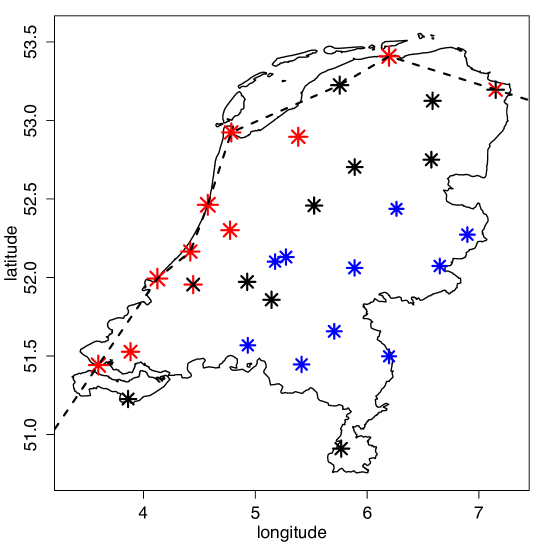
Figure 1: Measurement sites for wind gusts in the Netherlands. Coastal stations are connected with a dashed and piecewise linear curve. Each site is marked with a $+$-symbol, whose size is proportional to the empirical $0.95$-quantile divided by the mean of all such quantiles, and a $\times$-symbol, whose size is proportional (with the same constant as for $0.95$-quantiles) to the empirical $0.99$-quantiles, divided by the mean of all such quantiles. In each case, the sites associated to the $10$ highest quantile values are marked in red, and the sites associated to the $10$ lowest quantile values are marked in blue.

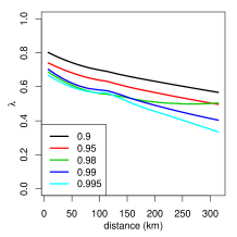
Figure 2: Exploratory plots. Left: LOESS-smoothed empirical tail correlation functions $\lambda$ with respect to intersite distance, estimated for different thresholds $u$. Right: Empirical estimates of the residual coefficient $\rho$ with respect to intersite distance and local regression curve (LOESS); pins indicate the orientation of the spatial lag.

4.2 Marginal modeling

The vast literature on wind speed modeling has identified the Weibull distribution as the most adequate candidate for univariate tails (Stevens and Smulders, 1979; Seguro and Lambert, 2000; Akdağ and Dinler, 2009). Therefore, we will not fit the classical tail model (2) and the related generalized Pareto distribution (3) for exceedances to univariate tails, but instead the Weibull distribution whose density is $x\mapsto 1_{[0,\infty)}(x)\gamma\delta^{-\gamma}x^{\gamma-1}\exp[-\{x/\delta\}^{\gamma}]$ with parameter constraints $\delta>0$ and $\gamma>0$. The Weibull distribution extends the classical tail model with shape $\xi=0$ (limit of Gumbel type) and mean $\mu=0$ by introducing a supplementary shape parameter $\gamma$; the classical model then applies to transformed data $x^{\gamma}$. We account for spatial variation by allowing the covariate “distance to the sea in km” to modify the value of the Weibull scale parameter $\delta=\exp(\delta_{0}+\delta_{1}\times\mathrm{covariate})$. For a fixed threshold $u>0$, the contribution of an observation $x$ to the independence likelihood of univariate tail parameters is

$$1(x\leq u)\times\left(1-\exp\left[-\{x/\delta\}^{\gamma}\right]\right)+1(x>u)\times\gamma\delta^{-\gamma}x^{\gamma-1}\exp\left[-\{x/\delta\}^{\gamma}\right].$$ (20)

In preliminary studies, we further tried to include a location parameter in a way similar to the classical tail model (2), i.e. replacing $x$ by $x-\mu$ with $\mu<u$ in (20), but we could not detect any substantial improvement in the goodness-of-fit and the numerical maximization of the likelihood became unstable. After fixing $u$ to the empirical $0.975$-quantile calculated from all observations, estimates and bootstrap-based confidence intervals of level $0.95$ are given as follows: ${\widehat{\gamma}}=1.72$($1.55,1.86$), ${\widehat{\delta}}_{0}=2.44$($2.29,2.52$) m/s and ${\widehat{\delta}}_{1}=-0.0021$($-0.0026,-0.0019$) m/s, where confidence intervals have been calculated from a block bootstrap sample (block size $30$, sample size $100$). The effect of distance to the sea $\delta_{1}$ is significantly different from $0$ and indicates that the strength of wind gusts weakens when we move away from the coastline. We follow common practice in spatial extreme value modeling and use the empirical distribution below the threshold by assuming dense observations in the bulk region of the distribution (Coles and Tawn, 1991; Wadsworth and Tawn, 2012, 2013).

4.3 Dependence modeling

We consider Gaussian and Laplace dependence models with correlation functions of exponential, stable or Matérn type. For the Matérn model, we tried out a selection of regularity parameters $\nu\in\{0.1,0.15,0.2,0.25,0.3,0.4,1,1.5,2.5,5\}$. We further allow geometric anisotropy to accommodate a potentially different scale of dependence along one direction, for instance stronger dependence orthogonal to the coastline for winds hitting land from the sea. By denoting $\theta\in[0,\pi)$ a rotation angle and $b\geq 1$ a stretching along this direction, we replace the original bivariate column distance vector $\Delta\bm{s}$ by the matrix product

$$\begin{pmatrix}b&0\\ 0&1\end{pmatrix}\begin{pmatrix}\cos(\theta)&-\sin(\theta)\\ \sin(\theta)&\cos(\theta)\end{pmatrix}\Delta\bm{s}=M\,\Delta\bm{s}.$$

Parameters $\theta$ and $b$ are estimated. We use Akaike’s information criterion AIC to select the best model. To make values of the censored likelihood (19) comparable for the Gaussian and the Laplace model, we first transform the original data $\bm{x}$ to $\tilde{\bm{x}}$ with uniform margins through the empirical transform for each of the $30$ sites. If $L(\bm{\theta};\bm{x})$ is the likelihood (19) for either Laplace or Gaussian margins, we use instead the likelihood $\tilde{L}$ in terms of $\tilde{\bm{x}}$,

$$\tilde{L}(\bm{\theta};\tilde{\bm{x}})=L(\bm{\theta};F^{-1}(\tilde{\bm{x}}))\times\prod_{i,j}(f(F^{-1}(\tilde{x}_{ij})))^{-1},\quad j=1,\ldots,30,\quad i=1,\ldots,3241,$$ (21)

where $F$ is either the standard Laplace or standard Gaussian cdf, and $f$ is the corresponding density.

Table 1 sums up the estimation results, where the highest AIC values $2\log\tilde{L}({\widehat{\bm{\theta}}};\tilde{\bm{x}})-2\,\mathrm{dim}({\widehat{\bm{\theta}}})$ of both the Laplace and Gaussian Matérn models were obtained for the shape parameter $\nu=0.25$. As before, standard errors have been calculated through the block bootstrap approach. When calculating AIC, we consider Matérn models with different values of $\nu$ as different models, such that $\nu$ is not counted for the model dimension. The shape parameters retained for the stable and the Matérn class indicate nondifferentiable trajectories. Geometric anisotropy improves AIC, but the improvement is relatively small compared to the differences between the three classes of correlation functions. Since ${\widehat{b}}>1$, we find that spatial dependence is weakest along the direction vector $(\cos({\widehat{\theta}}),\sin({\widehat{\theta}}))\approx(0.58,0.81)$, here calculated for the Matérn Laplace model, whereas it is strongest when we move orthogonally to this direction. This direction approximately follows the orientation of the coastline and we can conclude that winds hitting land from the sea (or the other way round) are stronger dependent in space. Throughout, Laplace models outperform their Gaussian counterpart. Overall, we select the Laplace model with the anisotropic Matérn correlation which obtains the highest AIC value. The Gaussian model with the same covariance family is second best. Since the isotropic Matérn correlation function attains the value $0.1$ approximately at distance $\sqrt{8\nu}\times\mathrm{scale}=\sqrt{2}\times\mathrm{scale}$, the estimated dependence is strong across the study region. For an illustration of the goodness-of-fit, we look at the quantile-quantile plots of the distribution of the sum of the observation vector above the $0.95$-quantiles in Figure 3. The sum distribution is a good choice since its tail decay behavior can be specified with an exact, nonasymptotic expression for elliptical distributions, see the results of Proposition 2 for the Laplace distribution. To facilitate the comparison of the displays for the Gaussian and the Laplace model, theoretical quantiles of the standard Laplace distribution are used and the data are transformed accordingly. For instance, the transformation of a data vector $\tilde{\bm{x}}_{i}=\tilde{x}_{ij}$, $j=1,\ldots,30$ as defined in (19) into its corresponding standard Laplace quantile $\tilde{q}_{i}$ is done as follows for the Gaussian model:

$$\tilde{q}_{i}=F^{-1}\left(\Phi\left(\sum_{j=1}^{30}\Phi^{-1}(\tilde{x}_{ij})/\sqrt{\bm{e}^{\prime}{\widehat{\Sigma}}\bm{e}}\right)\right),$$

where $F$ is the standard Laplace cdf and $\Phi$ is the standard Gaussian cdf. In both cases, data points are aligned close to the diagonal, with no strong differences between the Gaussian and the Laplace model. Figure 4 shows the difference of empirical and theoretical residual coefficients for these two models, with empiricial coefficients given as on the right-hand side of Figure 2. The local mean of differences has slightly positive values, which can at least partly be explained by second-order terms with respect to the asymptotic decay rate. Finally, Figure 5 contrasts the exact conditional exceedance probabilities $\lambda_{u}(s_{1},s_{2})=\mathrm{pr}(F_{X(s_{1})}(X(s_{1}))\geq u\mid F_{X(s_{2})}(X(s_{2}))\geq u)$ of the two models with the corresponding tail correlation estimates of data already presented on the left in Figure 2. Whereas the Laplace model convincingly reproduces the observed behavior in data, the Gaussian model is strongly biased towards too low values.

Covariance	Type	$\theta$	$b$	scale	shape	log-L	AIC
exp	G	$-$($-$)	$-$($-$)	369.0(22.44)	$-$($-$)	17420	34830
	L	$-$($-$)	$-$($-$)	376.6(18.43)	$-$($-$)	17620	35230
	G	0.42(0.2)	1.14(0.06)	384.3(11.61)	$-$($-$)	17430	34850
	L	1.02(0.15)	1.09(0.05)	381.9(7.7)	$-$($-$)	17630	35250
stable	G	$-$($-$)	$-$($-$)	3294(5.14)	0.53(0.01)	17740	35470
	L	$-$($-$)	$-$($-$)	3299(47.49)	0.50(0.01)	17890	35770
	G	0.89(0.11)	1.25(0.11)	3302(3.97)	0.54(0.02)	17750	35500
	L	1.14(0.1)	1.31(0.11)	3299(58.8)	0.52(0.01)	17930	35840
Matérn	G	$-$($-$)	$-$($-$)	3149(381.4)	0.25($-$)	17780	35560
	L	$-$($-$)	$-$($-$)	3087(297)	0.25($-$)	17900	35800
	G	0.87(0.12)	1.24(0.07)	3384(136.4)	0.25($-$)	18280	36550
	L	0.95(0.07)	1.41(0.09)	3698(121.7)	0.25($-$)	18440	36860

Table 1: Estimated tail models for max exceedances of the Netherlands wind gust data. “Type” is either G for the Gaussian likelihood or L for the Laplace likelihood. Standard errors have been calculated through a block bootstrap approach. For the calculation of Akaike’s criterion (AIC; here values are rounded to $4$ significant digits), the Matérn shape parameter is not considered as an estimated parameter.

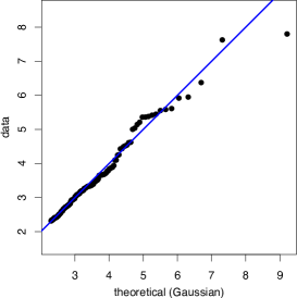
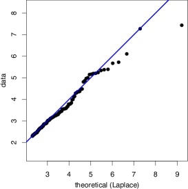
Figure 3: Quantile-quantile plots for sum exceedances above the $0.95$-quantile in the Gaussian (left display) and the Laplace (right display) tail dependence models with respect to the estimated Matérn correlation models. In both cases, the theoretical quantiles correspond to a standard Laplace tail and the data quantiles are transformed accordingly.

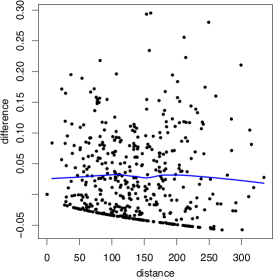
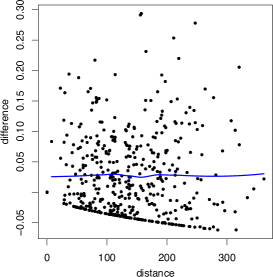
Figure 4: Difference of pairwise empirical estimates and theoretical values for the residual coefficient in the Gaussian (left) and the Laplace (right) tail dependence models with respect to the estimated Matérn correlation models. Distances have been corrected for anisotropy according to the estimated anisotropy matrices such that $\mathrm{dist}=\|M\Delta\bm{s}\|_{2}$.

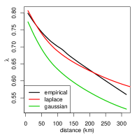
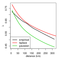
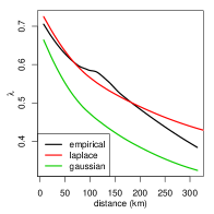
Figure 5: Comparison of conditional exceedance probabilities $\lambda_{u}$ between data and fitted Laplace and Gaussian models. From left to right for threshold values $u$ given by $\{0.9,0.95,0.99\}$. The curves for data correspond to the empirical smoothed tail correlation estimates presented on the left of Figure 2.

4.4 Conditional simulations and return levels/periods

To illustrate conditional simulation for the Laplace model according to the algorithm described at the end of Section 3.2, Figure 6 shows examples for two scenarios. In the first one, we condition on values at the $30$ sites observed on 18 January 2007 during the Kyrill storm, whose mean $32.4$ m/s is the highest over the observation period. In the second scenario, we condition on the estimated daily return level $x_{\mathrm{cond}}=51.0$ m/s of one of the coastal sites with respect to a long return period of 10000 years, i.e., $1/(365.25\times 10^{4})=\exp(-(x_{\mathrm{cond}}/{\widehat{\delta}})^{{\widehat{\gamma}}})$. The gradient of marginal scale with respect to distance to the sea is well perceptible in both simulations.

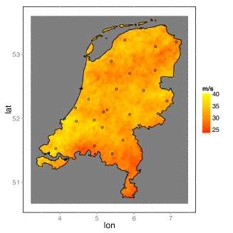
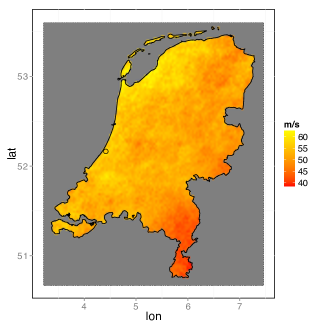
Figure 6: Conditional simulations. Left: conditional to highest daily mean observation, observed on 18 January 2007. Right: conditional to 10000 year daily return period of one coastal site. Points indicate the conditioning sites and their values.

Regarding the calculation of return periods and levels taking into account spatial dependence, we first consider the return period of an exceedance of the level $51$ m/s at at least one point in the Netherlands territory. Based on a fine spatial discretization $s_{1},\ldots,s_{345}$ of the Netherlands and the corresponding correlation matrix ${\widehat{\Sigma}}^{*}$ of the Laplace model, we calculate sitewise standard-scale values $\tilde{x}(s_{j})=1-\exp(-x_{0}/{\widehat{\delta}}(s_{j}))^{{\widehat{\gamma}}}$, $j=1,\ldots,345$ with $x_{0}=51$. Using formula (15) for numerical integration, the return period in years is

$$\mathrm{RP}(x_{0})={\textstyle{1\over 365.25\times\left(1-\int_{0}^{\infty}\Phi_{{\widehat{\Sigma}}^{*}}\left(\left(F^{-1}(\tilde{x}_{1}),\ldots,F^{-1}(\tilde{x}_{345})\right)/y\right)f_{Y}(y)\,\mathrm{d}y\right)}}=376,$$ (22)

where $F$ is the univariate standard Laplace distribution. Therefore, considering the whole country instead of a single site decreases the return period from $10000$ to $376$ years. We can further determine the return level associated to a return period of $10^{c}$ years ($c=0,1,2,3,4$) for the maximum observed over the whole territory. We numerically calculate the value $x_{0}^{*}$ for which the function $x_{0}\mapsto|\mathrm{RP}(x_{0})-10^{c}|$ attains its minimum $0$, yielding values (in m/s) $37.3$, $44.0$, $49.9$, $55.1$, $60.0$ for $c=0,1,2,3,4$ respectively.

5 Discussion and perspectives

Due to its generalized Pareto tails and the sum stability of its multivariate elliptical distributions, the Laplace tail model has advantageous properties for extreme value analysis while remaining close to the Gaussian processes used in classical geostatistics. For conditional and unconditional simulation in high dimensions, the well-studied Gaussian techniques are the main ingredient. Standard maximum likelihood inference is possible. In contrast to the Gaussian copula model, it is easier to interpret in the extreme value context since the elliptical structure arises for Laplace marginal distributions which, unlike the univariate Gaussian, are more natural for extremes. Moreover, the standardization to marginal Laplace distributions yields an exponential tail decay rate that is relatively close to the actually observed tail decay rates in environmental processes like wind speeds or precipitations.

The goodness-of-fit checks for wind gust data revealed a better fit of the Laplace model in terms of Akaike’s criterion and bivariate joint tail decay behavior. We did not take into account temporal dependence among extremes. A simple possibility for capturing clustering behavior in time would be to model the time series of a summary statistics like the sum of the marginally normalized observations at the observed time steps with models akin to the exponential ARMA processes of Lawrance and Lewis (1980).

The Gaussian scale mixture construction of Laplace models opens perspectives to more complex models. The latent exponential variance variables could be dependent over time or vary over space, which would then necessitate a Bayesian framework to handle latent variables. Finally, other than exponential variables $Y$ could be substituted for the variance of the Gaussian field. Such modeling would lead to higher flexibility in the extremal dependence structure with respect to tail decay rates, yet densities and cdfs are usually not available in closed form, and typically the resulting marginal distributions are not natural in the context of extremes.

6 Acknowledgements

The author is grateful to an editor and to two referees for numerous comments that helped improving the manuscript.

References

- Akdağ and Dinler (2009) Akdağ, S. A., Dinler, A., 2009. A new method to estimate Weibull parameters for wind energy applications. Energy conversion and management 50 (7), 1761–1766.
- Beirlant et al. (2004) Beirlant, J., Goegebeur, Y., Segers, J., Teugels, J., 2004. Statistics of Extremes: Theory and Applications. Wiley.
- Bortot et al. (2000) Bortot, P., Coles, S. G., Tawn, J. A., 2000. The multivariate Gaussian tail model: An application to oceanographic data. Journal of the Royal Statistical Society, Series C 49 (1), 31–049.
- Brodin and Rootzén (2009) Brodin, E., Rootzén, H., 2009. Univariate and bivariate GPD methods for predicting extreme wind storm losses. Insurance: Mathematics and Economics 44 (3), 345–356.
- Cambanis et al. (1981) Cambanis, S., Huang, S., Simons, G., 1981. On the theory of elliptically contoured distributions. Journal of Multivariate Analysis 11 (3), 368–385.
- Coles (2001) Coles, S. G., 2001. An Introduction to Statistical Modeling of Extreme Values. Springer.
- Coles and Tawn (1991) Coles, S. G., Tawn, J. A., 1991. Modelling extreme multivariate events. Journal of the Royal Statistical Society, Series B 53 (2), 377–392.
- Davison et al. (2013) Davison, A. C., Huser, R., Thibaud, E., 2013. Geostatistics of dependent and asymptotically independent extremes. Mathematical Geosciences 45 (5), 511–529.
- Davison et al. (2012) Davison, A. C., Padoan, S., Ribatet, M., 2012. Statistical modelling of spatial extremes. Statistical Science 27 (2), 161–186.
- de Carvalho and Davison (2014) de Carvalho, M., Davison, A. C., 2014. Spectral density ratio models for multivariate extremes. Journal of the American Statistical Association 109 (506), 764–776.
- de Haan and Ferreira (2006) de Haan, L., Ferreira, A., 2006. Extreme value theory: An introduction. Springer.
- Dhôte (2005) Dhôte, J.-F., 2005. Implication of forest diversity in resistance to strong winds. In: Forest diversity and function. Springer, pp. 291–307.
- Draisma et al. (2004) Draisma, G., Drees, H., Ferreira, A., de Haan, L., 2004. Bivariate tail estimation: dependence in asymptotic independence. Bernoulli 10 (2), 251–280.
- Einmahl et al. (2015) Einmahl, J., Kiriliouk, A., Krajina, A., Segers, J., 2015. An M-estimator of spatial tail dependence. Journal of the Royal Statistical Society, Series B. In press.
- Eltoft et al. (2006) Eltoft, T., Kim, T., Lee, T.-W., 2006. On the multivariate Laplace distribution. Signal Processing Letters, IEEE 13 (5), 300–303.
- Engelke et al. (2015) Engelke, S., Malinowski, A., Kabluchko, Z., Schlather, M., 2015. Estimation of Hüsler–Reiss distributions and Brown–Resnick processes. Journal of the Royal Statistical Society, Series B 77 (1), 239–265.
- Falk and Guillou (2008) Falk, M., Guillou, A., 2008. Peaks-over-threshold stability of multivariate generalized Pareto distributions. Journal of Multivariate Analysis 99 (4), 715–734.
- Genz and Bretz (2009) Genz, A., Bretz, F., 2009. Computation of multivariate normal and t probabilities. Springer, Berlin.
- Hashorva (2010) Hashorva, E., 2010. On the residual dependence index of elliptical distributions. Statistics & Probability Letters 80 (13), 1070–1078.
- Hill (1975) Hill, B. M., 1975. A simple general approach to inference about the tail of a distribution. Annals of Statistics 3 (5), 1163–1174.
- Kotz et al. (2001) Kotz, S., Kozubowski, T., Podgorski, K., 2001. The Laplace distribution and generalizations: a revisit with applications to communications, economics, engineering, and finance. Springer.
- Lawrance and Lewis (1980) Lawrance, A. J., Lewis, P. A. W., 1980. The exponential autoregressive-moving average EARMA(p,q) process. Journal of the Royal Statistical Society, Series B 42 (2), 150–161.
- Ledford and Tawn (1996) Ledford, A. W., Tawn, J. A., 1996. Statistics for near independence in multivariate extreme values. Biometrika 83 (1), 169.
- Ledford and Tawn (1997) Ledford, A. W., Tawn, J. A., 1997. Modelling dependence within joint tail regions. Journal of the Royal Statistical Society, Series B 59 (2), 475–499.
- Mornet et al. (2015) Mornet, A., Opitz, T., Luzi, M., Loisel, S., 2015. Index for predicting insurance claims from wind storms with an application in France. Risk Analysis. In press.
- Nagel et al. (2006) Nagel, T. A., Svoboda, M., Diaci, J., 2006. Regeneration patterns after intermediate wind disturbance in an old-growth Fagus–Abies forest in southeastern Slovenia. Forest Ecology and management 226 (1), 268–278.
- Nolde (2014) Nolde, N., 2014. Geometric interpretation of the residual dependence coefficient. Journal of Multivariate Analysis 123, 85–95.
- Oesting et al. (2015) Oesting, M., Schlather, M., Friederichs, P., 2015. Statistical post-processing of forecasts for extremes using bivariate Brown–Resnick processes with an application to wind gusts, http://arxiv.org/abs/1312.4584.
- Opitz (2013a) Opitz, T., 2013a. Extremal t processes: Elliptical domain of attraction and a spectral representation. Journal of Multivariate Analysis 122, 409–413.
- Opitz (2013b) Opitz, T., 2013b. Extrêmes multivariés et spatiaux: approches spectrales et modèles elliptiques. Ph.D. thesis, École doctorale I2S – Information, Structures, Systèmes, Montpellier, France, 146 pages.
- Opitz et al. (2015) Opitz, T., Bacro, J.-N., Ribereau, P., 2015. The spectrogram: A threshold-based inferential tool for extremes of stochastic processes. Electronic Journal of Statistics 9, 842–868.
- Pontailler et al. (1997) Pontailler, J.-Y., Faille, A., Lemée, G., 1997. Storms drive successional dynamics in natural forests: a case study in Fontainebleau forest (France). Forest Ecology and Management 98 (1), 1–15.
-
R Core Team (2013)
R Core Team, 2013. R: A Language and Environment for Statistical Computing. R
Foundation for Statistical Computing, Vienna, Austria.
URL http://www.R-project.org/ - Ramos and Ledford (2009) Ramos, A., Ledford, A., 2009. A new class of models for bivariate joint tails. Journal of the Royal Statistical Society, Series B 71 (1), 219–241.
- Renard and Lang (2007) Renard, B., Lang, M., 2007. Use of a Gaussian copula for multivariate extreme value analysis: some case studies in hydrology. Advances in Water Resources 30 (4), 897–912.
- Resnick (1987) Resnick, S. I., 1987. Extreme values, regular variation and point processes. Springer.
- Schlather and Tawn (2003) Schlather, M., Tawn, J. A., 2003. A dependence measure for multivariate and spatial extreme values: Properties and inference. Biometrika 90 (1), 139–156.
- Seguro and Lambert (2000) Seguro, J. V., Lambert, T. W., 2000. Modern estimation of the parameters of the Weibull wind speed distribution for wind energy analysis. Journal of Wind Engineering and Industrial Aerodynamics 85 (1), 75–84.
- Steinkohl et al. (2013) Steinkohl, C., Davis, R. A., Klüppelberg, C., 2013. Extreme value analysis of multivariate high-frequency wind speed data. Journal of Statistical Theory and Practice 7 (1), 73–94.
- Stevens and Smulders (1979) Stevens, M. J. M., Smulders, P. T., 1979. The estimation of the parameters of the Weibull wind speed distribution for wind energy utilization purposes. Wind engineering 3, 132–145.
- Strokorb et al. (2015) Strokorb, K., Ballani, F., Schlather, M., 2015. Tail correlation functions of max-stable processes. Extremes. In press.
- Thibaud et al. (2013) Thibaud, E., Mutzner, R., Davison, A. C., 2013. Threshold modeling of extreme spatial rainfall. Water Resources Research 49 (8), 4633–4644.
- Wadsworth and Tawn (2012) Wadsworth, J. L., Tawn, J. A., 2012. Dependence modelling for spatial extremes. Biometrika 99 (2), 253–272.
- Wadsworth and Tawn (2013) Wadsworth, J. L., Tawn, J. A., 2013. A new representation for multivariate tail probabilities. Bernoulli 19 (5), 2689–2714.
- Wadsworth et al. (2014) Wadsworth, J. L., Tawn, J. A., Davison, A. C., Elton, D., 2014. Modelling across extremal dependence classes, http://arxiv.org/abs/1408.5060.
- (1)