$J=0$ fixed pole and $D$-term form factor in deeply virtual Compton scattering

Abstract

S. Brodsky, F. J. Llanes-Estrada, and A. Szczepaniak emphasized the importance of the $J=0$ fixed pole manifestation in real and (deeply) virtual Compton scattering measurements and argued that the $J=0$ fixed pole is universal, i.e., independent on the photon virtualities Brodsky:2008qu . In this paper we review the $J=0$ fixed pole issue in deeply virtual Compton scattering. We employ the dispersive approach to derive the sum rule that connects the $J=0$ fixed pole contribution and the subtraction constant, called the $D$-term form factor for deeply virtual Compton scattering. We show that in the Bjorken limit the $J=0$ fixed pole universality hypothesis is equivalent to the conjecture that the $D$-term form factor is given by the inverse moment sum rule for the Compton form factor. This implies that the $D$-term is an inherent part of corresponding generalized parton distribution (GPD). Any supplementary $D$-term added to a GPD results in an additional $J=0$ fixed pole contribution and implies the violation of the universality hypothesis. We argue that there exists no theoretical proof for the $J=0$ fixed pole universality conjecture.

I Introduction

Compton scattering off a nucleon

$$\gamma^{(\ast)}(q_{1})+N(p_{1})\to\gamma^{(\ast)}(q_{2})+N(p_{2})$$ (1.1)

with real photons ($q_{1}^{2}=q_{2}^{2}=0$), with one virtual space-like and one real photon ($q_{1}^{2}=-Q_{1}^{2}<0$, $q_{2}^{2}=0$), and with two virtual space-like photons ($q_{1}^{2}=-Q_{1}^{2}<0$, $q_{2}^{2}=-Q_{2}^{2}<0$ ) are important processes to address the internal structure of nucleons from the low energy to the high energy regime. Depending on the resolution scale which is set up experimentally, different theoretical frameworks are appropriate to analyze experimental data and to provide interpretation in terms of the proper degrees of freedom.

Experimental and theoretical investigations of real Compton scattering are going back to pre-QCD time and were mainly based on the dispersive approach and the SO$(3)$ partial wave expansion in terms of the cross-channel angular momentum $J$. In particular, in the high energy region Regge theory was extensively employed. This implies that the high energy asymptotic behavior $s^{\alpha(t)}$ of the amplitude is determined by the (leading) Regge trajectory $\alpha(t)$, which depends on the momentum transfer squared $t=(p_{2}-p_{1})^{2}$. It is assumed that the corresponding partial wave amplitudes are analytic functions of $J$. Leading Regge behavior then originates from moving poles in the complex $J$-plane. Besides such moving poles there also might exist so-called fixed pole singularities (see e.g. Chapter I of Ref. Alfaro_red_book ) which

•  do not move with the change of $t$;

•  can not be revealed by means of the analytic continuation in $J$.

A $J=J_{0}$ fixed pole singularity may arise from a cross channel exchange with a non-Reggeized (elementary) particle of spin $J_{0}$ in the cross channel (or from a contact interaction term). It is then manifest as the Kronecker-$\delta$ singularity in the complex $J$-plane. Its $t$-channel quantum numbers might be exemplified e.g. by means of the Froissart-Gribov projection Gribov1961 ; Froissart1961 .

To our best knowledge, a $J=0$ fixed pole in the context of Compton scattering off proton first arose in Ref. Creutz:1968ds by M.J. Creutz, S.D. Drell, and E.A. Pashos as a constant, denoted here as $C_{\infty}$, in the Regge-pole representation of the real forward Compton scattering amplitude

$$f_{1}(\nu)=\sum_{\alpha\neq 0\atop\alpha\leq 1}\frac{\beta_{\alpha}\nu^{\alpha}}{4\pi}\;\frac{-1-e^{-i\pi\alpha}}{\sin(\pi\alpha)}+C_{\infty},$$ (1.2)

where the energy variable is $\nu=\frac{s-u}{4M}$. The representation (1.2) is supposed to be valid for the high energy region, while for low energy the Compton amplitude $f_{1}(\nu)$ is known to satisfy the Thomson limit

$$f_{1}(0)=\lim_{\nu\to 0}f_{1}(\nu)=-\frac{e_{p}^{2}}{4\pi M},$$ (1.3)

where $e_{p}$ is the electric charge and $M$ is the proton mass. Therefore, in a loose sense, the value of $C_{\infty}$ in (1.2) characterizes how much from the Thomson limit (1.3) survives in the high energy regime. In Ref. Damashek:1969xj , employing the subtracted dispersion relation of Gell-Mann, Goldberger, and Thirring GellMann:1954db , this was equivalently formulated in a more abstractly mathematical manner as the $J=0$ fixed pole sum rule expressed in terms of an analytically regularized inverse moment

$$C_{\infty}=f_{1}(0)-\frac{2}{\pi}\int_{\nu_{\rm thr}}^{(\infty)}\frac{d\nu}{\nu}{\rm Im}f_{1}(\nu),$$ (1.4)

where the absorptive part is given by the total photoabsorbtion cross section ${\rm Im}f_{1}(\nu)=\frac{\nu}{4\pi}\sigma_{T}(\nu)$. First attempts Damashek:1969xj ; Dominguez:1970wu to extract the value of $J=0$ fixed pole contribution at $t=0$ from experimental measurements employing finite–energy sum rules based on (1.4) found its value roughly consistent with the Thomson limit.

The manifestation of the $J=0$ fixed pole contribution for virtual Compton scattering, i.e. of the constant contribution in the high-energy asymptotic limit, was the subject of a broad discussion in the early seventies. S. Brodsky, F. Close and J. Gunion Brodsky:1971zh ; Brodsky:1972vv provided field theoretical arguments in favor of such contribution originating from local two-photon interaction corresponding at the diagrammatic level to the so-called “seagull” diagrams. A. Zee in Ref. Zee:1972nq argued that $J=0$ fixed pole is an inherent consequence of scaling behavior of the Compton amplitude in the Bjorken limit. However, this reasoning was criticized by M. Creutz Creutz:1973zf , who disclaimed the existence of any theoretical argument in favor of such singularity independent of specific models.

The importance of a $J=0$ fixed pole contribution has been anew emphasized more recently by S. Brodsky, F. J. Llanes-Estrada and A. Szczepaniak Brodsky:2008qu . They argue that this contribution possesses unique features that are absent in amplitudes of other processes such as meson production:

•  The $J=0$ fixed pole contribution is a $t$-dependent constant that is independent on the photon virtualities and is therefore universal.

•  In the parton model its value is given by the inverse moment of the corresponding $t$-dependent parton distribution function (PDF).

On the other hand, within the partonic picture, the subtraction constant, which appears in the transverse non-flip DVCS amplitude, originates from the so-called $D$-term. Originally, the $D$-term was introduced in Ref. Polyakov:1999gs as a separate addendum to a generalized parton distribution (GPD) that complements the polynomiality condition for the unpolarized charge even GPD $H^{(+)}$ within the double distribution representation Mueller:1998fv ; Radyushkin:1997ki . The existence of the $D$-term also has been justified from chiral dynamics. The first Mellin moment of the $D$-term contributes into the hadronic matrix elements of both the quark and gluon parts of the QCD energy momentum tensor. The negative value of this specific moment has been argued to be a necessity for the stability of the nucleon Polyakov:2002yz . It was realized that the $D$-term can be implemented as inherent part of GPD within the modified double distribution representation Belitsky:2000vk ; Teryaev:2001qm ; Radyushkin:2011dh . The $D$-term also turns to be a natural GPD ingredient within the GPD representation based on the double partial wave expansion (in conformal and in the cross-channel SO$(3)$ partial waves). This representation is known in two versions (the approach based on the Mellin-Barnes integral techniques of Ref. Mueller:2005ed , and the so-called dual parametrization approach Polyakov:2002wz ; Polyakov:2008aa ; SemenovTianShansky:2010zv ) that were recently found to be completely equivalent Muller:2014wxa . Within this approach it was first realized that the problem of universality of $J=0$ fixed pole is related to the analytic properties of GPD moments in the complex conformal spin $j$. The analyticity assumption requiring the absence of $j=-1$ fixed pole singularity in the Mellin space of spectral functions allows to express the subtraction constant through the analytically regularized inverse moment sum rule and turns to be equivalent to the $J=0$ fixed pole conjecture of Ref. Brodsky:2008qu .

In this paper we restrict ourselves to Compton scattering in the generalized Bjorken limit and provide a pedagogical presentation on the issue of $J=0$ fixed pole conjecture and the $D$-term representation. In Sec. II we review the derivation of fixed-$t$ dispersion relations for the Compton amplitude. We introduce a pair of equivalent dispersion relations: the standard subtracted one and the analytically regularized one. This provides the $J=0$ fixed pole sum rule in terms of the analytically regularized inverse moment. In Sec. III we employ these findings within the parton model to express the corresponding sum rule in terms of GPDs. We discuss the mathematical subtleties in taking the high energy limit of the $D$-term sum rule. In Sec. IV we show that the $J=0$ fixed pole conjecture holds true if the $D$-term is an inherent part of the GPD. This statement is illustrated with a toy GPD model example in Appendix A. Finally, in Sec. V we draw our conclusions.

II Dispersion approach for Compton scattering

II.1 Subtracted and unsubtracted dispersion relations for Compton amplitude

To parameterize the photon helicity amplitudes of Compton scattering (1.1) we adopt the notations and conventions of Ref. Belitsky:2012ch . In particular, the transverse non-flip photon helicity amplitude reads:

$${\cal T}_{++} \!\!\!=\!\!\! \overline{u}(p_{2})\Bigg{[}\frac{/\!\!\!\!P}{P\cdot q}{\cal H}(\nu,t|Q_{1}^{2},Q_{2}^{2})+i\sigma^{\alpha\beta}\frac{P_{\alpha}\Delta_{\beta}}{2M\,P\cdot q}$$

$$\phantom{\overline{u}\Bigg{[}\frac{/\!\!\!\!P}{P\cdot q}}\times{\cal E}(\nu,t|Q_{1}^{2},Q_{2}^{2})\Bigg{]}u(p_{1})+\mbox{parity odd part}\,,$$

where $\Delta=p_{2}-p_{1}$ and $\nu$ stands for the energy variable

$$\nu=\frac{P\cdot q}{2M}=\frac{s-u}{4M},\quad\mbox{with}\quad P=p_{1}+p_{2}\,,\quad q=\frac{1}{2}(q_{1}+q_{2})\,.$$ (2.2)

In what follows we mainly focus on the Compton form factor (CFF) ${\cal H}(\nu,t|Q_{1}^{2},Q_{2}^{2})$, the analog of the Dirac form factor, which has even signature (even parity and even charge conjugation parity), i.e., it is symmetric under the interchange of $\nu\to-\nu$.

•  In the forward kinematics ($Q_{1}^{2}=Q_{2}^{2}={\cal Q}^{2}$, $t=0$) its imaginary part corresponds to the deep inelastic scattering structure function $F_{1}$

$${\rm Im}\,{\cal H}(\nu,t=0|Q_{1}^{2}=Q_{2}^{2}={\cal Q}^{2})=2\pi F_{1}(x_{\rm B},{\cal Q}^{2}),$$ (2.3)

where $x_{\rm B}=\frac{{\cal Q}^{2}}{2M\nu}$.

•  For real Compton scattering it can be expressed through the transverse photoabsorbtion cross section

$${\rm Im}\,{\cal H}(\nu,t=0|Q_{1}^{2}=Q_{2}^{2}=0)=4\pi M\,{\rm Im}\,f_{1}(\nu)=M\nu\sigma_{T}(\nu).$$ (2.4)

         

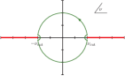
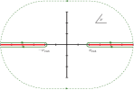
Figure 1: Left panel: Integration contour in the complex $\nu$ plane in eq. (2.5). Right panel: Deformation of the integration contour in eq. (2.6).

The derivation of fixed–$t$ dispersion relation (DR) for real photons or fixed space-like photon virtualities is based on the Cauchy theorem,

$${\cal H}(\nu,t|Q_{1}^{2},Q_{2}^{2})=\frac{1}{2\pi i}\oint d\nu^{\prime}\frac{1}{\nu^{\prime}-\nu}{\cal H}(\nu^{\prime},t|Q_{1}^{2},Q_{2}^{2}),\,$$ (2.5)

(see left panel in Fig. 1) and standard assumptions on the analytic structure of the CFF. In the following we concentrate on the Bjorken limit. Therefore, the Born term can be safely neglected and only the cuts along the real axis $[-\infty,-\nu_{\rm cut}]$ and $[\nu_{\rm cut},\infty]$, which start at the pion production threshold,

$$\nu_{\rm cut}=\frac{Q_{1}^{2}+Q_{2}^{2}+t+(M+2m_{\pi})^{2}-M^{2}}{4M}$$

are to be accounted. Deforming the integration contour in (2.5) as shown in the right panel of Fig. 1, and assuming that ${\cal H}$ vanishes at infinity ($\lim_{|\nu|\to\infty}{\cal H}(\nu,t|Q_{1}^{2},Q_{2}^{2})=0$), we work out the unsubtracted DR in the standard form,

$${\cal H}(\nu,t|Q_{1}^{2},Q_{2}^{2})=\frac{1}{\pi}\int^{\infty}_{\nu_{\rm cut}}d\nu^{\prime}\frac{2\nu^{\prime}\,{\rm Im}\,{\cal H}(\nu^{\prime},t|Q_{1}^{2},Q_{2}^{2})}{\nu^{\prime 2}-\nu^{2}-i\epsilon}.$$ (2.6)

If ${\cal H}$ does not vanish at infinity, the unsubtracted DR (2.5) still formally provides the correct result once the contributions from the large semi-circles are retained. However, it is practically of little use, since both the dispersive integral along the cuts and the contribution from the large semi-circles are divergent. Therefore, if one prefers to work with unsubtracted DR, e.g., as done in Ref. Brodsky:2008qu , it is indispensable to specify a regularization procedure at the point $\nu=\infty$.

A possible choice, which was already briefly discussed in the Introduction, is the analytic regularization. Here, the integration contour of the dispersive integral is deformed in a way that the integral along the real axis is replaced by the loop integral in the complex plane that includes the point $\nu=\infty$, denoted as $(\infty)$, for details see, e.g., Ref. GelShi64 . The unsubtracted DR (2.5) then reads

$${\cal H}(\nu,t|Q_{1}^{2},Q_{2}^{2}) \!\!\!=\!\!\! {\cal H}_{\infty}(t|Q_{1}^{2},Q_{2}^{2})$$

$$+\frac{1}{\pi}\int^{(\infty)}_{\nu_{\rm cut}}d\nu^{\prime}\frac{2\nu^{\prime}\,{\rm Im}\,{\cal H}(\nu^{\prime},t|Q_{1}^{2},Q_{2}^{2})}{\nu^{\prime 2}-\nu^{2}-i\epsilon},$$

where the constant ${\cal H}_{\infty}$, arising from the analytic regularization at $\nu=\infty$, turns to be the analog of $C_{\infty}$ in the expansion of the real forward Compton scattering amplitude (1.2). Within the Regge–pole expansion of the amplitude it is interpreted as the $J=0$ fixed pole contribution.

However, the analytically regularized DRs can be employed only once the analytic form of the spectral function is explicitly known. Therefore, the conventional form of DR employed within the deeply virtual (d.v.) regime is the subtracted DR with the subtraction taken at the unphysical point $\nu=0$:

$${\cal H}(\nu,t|Q_{1}^{2},Q_{2}^{2}) \!\!\!\stackrel{{\scriptstyle\rm d.v.}}{{=}}\!\!\! {\cal H}_{0}(t|Q_{1}^{2},Q_{2}^{2})$$

$$+\frac{1}{\pi}\int^{\infty}_{\nu_{\rm cut}}\frac{d\nu^{\prime}}{\nu^{\prime}}\frac{2\nu^{2}\,{\rm Im}\,{\cal H}(\nu^{\prime},t|Q_{1}^{2},Q_{2}^{2})}{\nu^{\prime 2}-\nu^{2}-i\epsilon}.$$

The detailed derivation of (II.1) is given, e.g., in Sec. 2.2 of Ref. Kumericki:2007sa ).

The dispersion relations (II.1) and (II.1) are supposed to represent the same function. Therefore, the $J=0$ fixed pole contribution ${\cal H}_{\infty}$ could be related to the subtraction constant ${\cal H}_{0}$. Plugging in the algebraic decomposition

$$\frac{2\nu^{\prime}}{\nu^{\prime 2}-\nu^{2}-i\epsilon}=\frac{1}{\nu^{\prime}}\frac{2\nu^{2}}{\nu^{\prime 2}-\nu^{2}-i\epsilon}+\frac{2}{\nu^{\prime}}$$

of the Cauchy kernel into (II.1) and comparing it with (II.1), we read off the sum rule

$${\cal H}_{\infty}(t|Q_{1}^{2},Q_{2}^{2}) \!\!\!=\!\!\! {\cal H}_{0}(t|Q_{1}^{2},Q_{2}^{2})$$

$$-\frac{2}{\pi}\int^{(\infty)}_{\nu_{\rm cut}}\frac{d\nu}{\nu}\,{\rm Im}{\cal H}(\nu,t|Q_{1}^{2},Q_{2}^{2})\,,$$

expressing the $J=0$ fixed pole contribution through the subtraction constant and the analytically regularized inverse moment of the absorptive part of the amplitude.

II.2 Dispersive approach in the scaling regime

In general, the subtraction constant ${\cal H}_{0}(t|Q_{1}^{2},Q_{2}^{2})$ of the DR (II.1) represents an unknown quantity. However, in the deeply virtual regime one can rely on the operator product expansion and formulate the external principle allowing to fix the value of the subtraction constant from the absorptive part. In particular, within the leading twist-two approximation current conservation ensures that for equal photon virtualities the subtraction constant vanishes: ${\cal H}_{0}(t|Q_{1}^{2}=Q_{2}^{2}={\cal Q}^{2})\stackrel{{\scriptstyle\rm d.v.}}{{=}}0$ (see Sec. 3.2.2 of Ref. Kumericki:2007sa for the detailed discussion), while in the DVCS kinematics the subtraction constant corresponds to the $D$-term form factor ${\cal H}_{0}(t|Q_{1}^{2}={\cal Q}^{2},Q_{2}^{2}=0)\stackrel{{\scriptstyle\rm d.v.}}{{=}}4{\cal D}(t)$.

Furthermore, in the framework of the operator product expansion it has been conjectured in Ref. Kumericki:2007sa that in absence of the $\delta_{j,-1}$ Kronecker singularity (also called as $j=-1$ fixed pole contribution) in the Mellin space of moments of the spectral function, the subtraction constant ${\cal H}_{0}(t|Q_{1}^{2},Q_{2}^{2})$ for nonequal photon virtualities can be evaluated from the analytically regularized inverse moment of the spectral function to leading twist accuracy to any order of perturbation theory. Within the convention used here, Eq. (47) of Ref. Kumericki:2007sa reads

$${\cal H}_{0}(t|Q_{1}^{2},Q_{2}^{2}) \!\!\!=\!\!\! \frac{2}{\pi}\int^{(\infty)}_{\nu_{\rm cut}}\frac{d\nu}{\nu}$$

$$\times{\rm Im}\left[{\cal H}(\nu,t|Q_{1}^{2},Q_{2}^{2})-{\cal H}(\nu,t|Q_{1}^{2}=Q_{2}^{2})\right],$$

where the inverse $\nu$-moment is computed by the analytic continuation of $\nu$-Mellin moments.

Plugging this conjectured inverse moment sum rule (II.2) into the expression (II.1) for the $J=0$ fixed pole contribution, one realizes that the $J=0$ fixed pole is independent on the ratio of photon virtualities and can be calculated from the equal photon virtuality case, yielding the conjecture of Ref. Brodsky:2008qu :

$${\cal H}_{\infty}(t|Q_{1}^{2},Q_{2}^{2})=-\frac{2}{\pi}\int^{(\infty)}_{\nu_{\rm cut}}\frac{d\nu}{\nu}\,{\rm Im}{\cal H}(\nu,t|Q_{1}^{2}=Q_{2}^{2})\,.$$ (2.11)

Within the deeply virtual kinematics regime it is convenient to rewrite the DRs of the previous subsection in terms of scaling variables. A natural choice is to use the Bjorken-like variable $\xi$ and the skewness related scaling variable $\eta$:

$$\xi=\frac{Q^{2}}{P\cdot q}=\frac{Q^{2}}{2M\nu};\,\qquad\eta=-\frac{\Delta\cdot q}{P\cdot q}=-\frac{\Delta\cdot q}{2M\nu}\,,$$ (2.12)

where $Q^{2}=-q^{2}\equiv-\frac{(q_{1}+q_{2})^{2}}{4}$. Here, instead of the scaling variable $\eta$, we employ the photon asymmetry parameter

$$\vartheta\equiv\eta/\xi=\frac{q_{1}^{2}-q_{2}^{2}}{q_{1}^{2}+q_{2}^{2}}+{\cal O}(t/Q^{2}),$$ (2.13)

which does not depend on the energy variable $\nu$ .

•  For $t=0$, the $\vartheta=0$ case corresponds to the usual DIS •  kinematics.

•  The case $\vartheta=1$ corresponds to the DVCS kinematics.

Within the scaling variables (2.12) the analytically regularized DR (II.1) and the subtracted one (II.1) read as follows:

$${\cal H}(\xi,t|\vartheta) \!\!\!=\!\!\! \frac{1}{\pi}\int^{1}_{(0)}\frac{d\xi^{\prime}}{\xi^{\prime}}\frac{2\xi^{2}\,{\rm Im}{\cal H}(\xi^{\prime},t|\vartheta)}{\xi^{2}-\xi^{\prime 2}-i\epsilon}+{\cal H}_{\infty}(t|\vartheta),\qquad$$ (2.14)

$${\cal H}(\xi,t|\vartheta) \!\!\!=\!\!\! \frac{1}{\pi}\int^{1}_{0}d\xi^{\prime}\frac{2\xi^{\prime}\,{\rm Im}{\cal H}(\xi^{\prime},t|\vartheta)}{\xi^{2}-\xi^{\prime 2}-i\epsilon}+{\cal H}_{0}(t|\vartheta)\,.$$ (2.15)

Here, the upper integration limit, given by $\xi_{\rm cut}=\frac{Q^{2}}{2M\nu_{\rm cut}}$, has been set in the (generalized) Bjorken limit to $\xi_{\rm cut}=1$ and the lower integration limit, $\xi=0$, corresponds to $\nu=\infty$. We emphasize that although the spectral function grows with increasing $\xi^{\prime}$, the analytically regularized DR (2.14) can be evaluated so far its small-$\xi^{\prime}$ asymptotic is analytically known. The equivalence of the two DRs (2.14), (2.15) is ensured by the sum rule (II.1), which now reads

$${\cal H}_{\infty}(t|\vartheta) \!\!\!=\!\!\! {\cal H}_{0}(t|\vartheta)-\frac{2}{\pi}\int^{1}_{(0)}\frac{d\xi}{\xi}\,{\rm Im}{\cal H}(\xi,t|\vartheta)\,.$$ (2.16)

III Dispersive versus pQCD approach

In this section, within the GPD framework set up in the familiar momentum fraction representation, we point out the origin of the additional fixed pole contribution $\Delta{\cal H}_{\infty}$, which eventually violates the $J=0$ fixed pole universality conjecture (2.11). In this approach, to the leading order (LO) accuracy, the CFF ${\cal H}(\xi,t|\vartheta)$ arises from the elementary amplitude

$${\cal H}(\xi,t|\vartheta)\stackrel{{\scriptstyle\rm LO}}{{=}}\int_{0}^{1}\!dx\,\frac{2x}{\xi^{2}-x^{2}-i\epsilon}H^{(+)}(x,\eta=\vartheta\xi,t)\,,$$ (3.1)

where $H^{(+)}(x,\eta,t)=H(x,\eta,t)-H(-x,\eta,t)$ stands for the antisymmetric charge even quark GPD combination. The imaginary part of the CFF is given by the GPD value in the outer region $\xi\geq\eta=\xi\vartheta$ for all allowed values $|\vartheta|\leq 1$,

$$\frac{1}{\pi}{\rm Im}{\cal H}(\xi,t|\vartheta)\stackrel{{\scriptstyle\rm LO}}{{=}}H^{(+)}(x=\xi,\eta=\xi\vartheta,t)\,.$$ (3.2)

Inserting the imaginary part (3.2) into the sum rule (2.16) allows to express the $J=0$ fixed pole contribution ${\cal H}_{\infty}(t|\vartheta)$ to LO accuracy by the GPD in the outer region:

$${\cal H}_{\infty}(t|\vartheta)\stackrel{{\scriptstyle\rm LO}}{{=}}{\cal H}_{0}(t|\vartheta)-2\int^{1}_{(0)}\frac{dx}{x}\,H^{(+)}(x,\vartheta x,t)\,.$$ (3.3)

Now, by plugging the imaginary part (3.2) into the subtracted DR (2.15) and equating it with the LO convolution formula (3.1) for the CFF, we obtain the GPD sum rule Kumericki:2008di , which was originally worked out within the double distribution representation Teryaev:2005uj ; Anikin:2007yh :

$$4{\cal D}(t|\vartheta)\stackrel{{\scriptstyle\rm LO}}{{=}}\int_{0}^{1}\!dx\frac{2x}{x^{2}-\xi^{2}}\!\left[\!H^{(+)}(x,\vartheta x,t)-H^{(+)}(x,\vartheta\xi,t)\right]$$ (3.4)

for the $D$-term form factor. Note that for $\xi\neq 0$ the integrand in (3.4) has an integrable singularity at $x=\xi$. The spectral function $H^{(+)}(x,\vartheta x,t)$ has a branch point at $x=0$, while the GPD $H^{(+)}(x,\vartheta\xi,t)$ has a branch point at $x=\vartheta\xi$ and vanishes at $x=0$ due to antisymmetry in $x$. The sum rule (3.4) is valid for all values of $\xi$ , where the special values $\xi\in\{0,1,1/\vartheta,\infty\}$ should be approached in special limiting procedures (see Ref. Kumericki:2008di for a more detailed discussion).

•  The low energy limit $\xi\to\infty$ of (3.4) is rather uncritical: the DR integral drops out and $D$-term form factor is given in terms of the $D$-term $d(x,t)$ that is here defined as a limiting value of the GPD:

$$4{\cal D}(t|\vartheta) \!\!\!\stackrel{{\scriptstyle\rm LO}}{{=}}\!\!\! \int_{0}^{1}\!dx\,\frac{2x\vartheta^{2}}{1-x^{2}\vartheta^{2}}\,d(x,t)$$ (3.5)

with $$d(x,t)=\lim_{\xi\to\infty}H^{(+)}(\xi x,\xi,t)\,.$$

•  Contrarily, the high energy limit $\xi\to 0$ of (3.4) requires special attention. At a first glance this limit looks tempting to provide a proof for the $J=0$ fixed pole conjecture of Ref. Brodsky:2008qu . However, we would like to stress that interchanging the integration and limiting procedure can render a wrong result, since a squeezed contribution from the central GPD region might be missed.

Let us consider the popular GPD representation in which the $D$-term (denoted as $d^{\rm f.p.}$) is an addenda that completes polynomiality Polyakov:1999gs :

$$H^{(+)}(x,\eta,t)=H_{\rm DD}^{(+)}(x,\eta,t)+\theta(|\eta|-|x|)d^{\rm f.p.}(x/|\eta|,t)\,,$$ (3.6)

where $H_{\rm DD}^{(+)}$ has the rather common double distribution representation, see below Eq. 4.1 for $a=0$. In the $N$-th Mellin moment $\int_{-1}^{1}\!dx\,x^{N}H_{\rm DD}^{(+)}(x,\eta,t)$ of the GPD the highest possible power in $\eta^{N+1}$ for odd $N$ is missing. We would like to show that the $D$-term addenda in (3.6) can be interpreted as the $J=0$ fixed pole contribution violating the $J=0$ fixed pole sum rule conjectured in Ref. Brodsky:2008qu . For simplicity, let us suppose that both the CFF spectral function $H_{\rm DD}^{(+)}(x,\vartheta x,t)$ and the GPD $H_{\rm DD}^{(+)}(x,\vartheta\xi,t)$ vanish at $x=0$, allowing us to interchange safely the integration and $\xi\to 0$ limiting procedure in (3.4). We plug the GPD (3.6) into the $D$-term form factor sum rule (3.4), and separate the integration region into the central, $x\in[0,\vartheta\xi]$, and outer, $x\in[\vartheta\xi,1]$, GPD regions. Then taking the high energy limit $\xi\to 0$, we find that the corresponding sum rule reads

$$4{\cal D}(t|\vartheta) \!\!\!\stackrel{{\scriptstyle\rm LO}}{{=}}\!\!\! 2\int_{0}^{1}\!\frac{dx}{x}\!\left[\!H_{\rm DD}^{(+)}(x,\vartheta x,t)-q^{(+)}(x,t)\right]\quad$$

$$+4{\cal D}^{\rm f.p.}(t|\vartheta),$$

where $q^{(+)}(x,t)\equiv H_{\rm DD}^{(+)}(x,0,t)$ stands for the corresponding $t$-dependent PDF (we assume that $q^{(+)}(x=0,t)=0$ to ensure convergence of the integral) and

$$4{\cal D}^{\rm f.p.}(t|\vartheta) \!\!\!\stackrel{{\scriptstyle\rm LO}}{{=}}\!\!\! \lim_{\xi\to 0}\int_{0}^{\vartheta\xi}\!dx\,\frac{2x}{\xi^{2}-x^{2}}\,d^{\rm f.p.}\!\left(\!\frac{x}{\vartheta\xi}\!,t\right)$$

$$\!\!\!\stackrel{{\scriptstyle\rm LO}}{{=}}\!\!\! \int_{0}^{1}\!dx\,\frac{2x\vartheta^{2}}{1-\vartheta^{2}x^{2}}\,d^{\rm f.p.}(x,t)\,.$$

Note that since by construction the $d^{\rm f.p.}$ term provides the complete contribution to the $D$-term form factor, the inverse moment of the GPD/PDF combination in (III) vanishes.

Now, inserting the $D$-term form factor (III) into (3.3), we conclude that in addition to the universal inverse PDF moment the subtraction constant ${\cal H}_{\infty}(t|\vartheta)$ receives an additional non-universal contribution from the $D$-term $d^{\rm f.p.}(x)$, defined solely within the GPD central region:

$${\cal H}_{\infty}(t|\vartheta)\stackrel{{\scriptstyle\rm LO}}{{=}}-2\int^{1}_{0}\frac{dx}{x}\,q^{(+)}(x,t)+\underbrace{4{\cal D}^{\rm f.p.}(t|\vartheta)}_{\Delta{\cal H}_{\infty}(t|\vartheta)}\,.$$ (3.9)

Note that the additional $J=0$ fixed pole contribution $\Delta{\cal H}_{\infty}(t|\vartheta)$, depends on the photon virtualities and is therefore non-universal.

•  Therefore, we conclude that on general ground the GPD sum rule (3.4) can not deliver a proof for the conjecture (II.2) that the subtraction constant ($D$-term form factor) can be evaluated from an inverse moment of the spectral function and so the $J=0$ fixed pole (2.11) universality conjecture remains also unproved.

•  We also add that the high energy limit $\xi\to 0$ and integration procedure in the GPD sum rule (3.4) can not be interchanged in the presence of Regge behavior. Neglecting the central GPD region now implies that one also throws away divergent terms that are needed to render a finite $D$-term form factor result.

A particular example of a GPD model with a non-zero $j=-1$ fixed pole contribution is provided by the calculation SemenovTianShansky:2008mp of pion GPDs in the non-local chiral quark model Praszalowicz:2003pr . In this model the universality conjecture (2.11) is not valid due to a supplementary $J=0$ fixed pole contribution originating from the $D$-term $d^{\rm f.p.}(x,t)$, which has to be added to make GPD satisfy the soft pion theorem Pobylitsa:2001cz fixing pion GPDs in the limit $\eta\to 1$.

Now we are about to spell out the relation between the $J=0$ fixed pole contribution and the $D$-term form factor ${\cal D}(t|\vartheta)$ making special emphasize on the two kinds of analytical properties relevant for GPDs and associated CFFs:

•  analyticity of CFFs in the cross channel angular momentum $J$;

•  analyticity of GPD Gegenbauer/Mellin moments in the variable $j$, labeling the conformal spin $j+2$ of twist-$2$ quark conformal basis operators

$${\cal O}_{j}^{a}=\frac{\Gamma(3/2)\Gamma(1+j)}{2^{j}\Gamma(3/2+j)}\,(i\!\stackrel{{\scriptstyle\leftrightarrow}}{{\partial}}_{+})^{j}\;\bar{\psi}\lambda^{a}\gamma_{+}\,C_{j}^{3/2}\!\left(\!\frac{\stackrel{{\scriptstyle\leftrightarrow}}{{D}}_{+}}{\stackrel{{\scriptstyle\leftrightarrow}}{{\partial}}_{+}}\!\right)\psi.$$ (3.10)

To deal with $J$ analytical properties of CFFs, following Sec. 6.3 of Ref. Muller:2014wxa , it is instructive to consider the Froissart-Gribov projection Gribov1961 ; Froissart1961 of the cross channel SO$(3)$ PWs of the CFF ${\cal H}(\xi,t|\vartheta)$:

$$a_{J}(t|\vartheta)\equiv\frac{1}{2}\int_{-1}^{1}\!d(\cos\theta_{t})\,P_{J}(\cos\theta_{t}){\cal H}^{(+)}(\cos\theta_{t},t|\vartheta),$$ (3.11)

where, neglecting the threshold corrections $\sim\sqrt{1-\frac{4M^{2}}{t}}$,

$$\cos\theta_{t}=-\frac{1}{\vartheta\xi}+{\cal O}(1/Q^{2}).$$

For $J>0$ PWs the Froissart-Gribov projection provides to LO accuracy

$$a_{J>0}(t|\vartheta)\stackrel{{\scriptstyle\rm LO}}{{=}}2\int_{0}^{1}\!dx\frac{{\cal Q}_{J}(1/x)}{x^{2}}H^{(+)}(x,\vartheta x,t)\,,$$ (3.12)

where ${\cal Q}_{J}(1/x)$ stand for the Legendre functions of the second kind. For $J=0$ one obtains

$$a_{J=0}(t|\vartheta) \!\!\!\stackrel{{\scriptstyle\rm LO}}{{=}}\!\!\! 2\int_{0}^{1}\!dx\left[\frac{{\cal Q}_{0}(1/x)}{x^{2}}-\frac{1}{x}\right]H^{(+)}(x,\vartheta x,t)$$ (3.13)

$$+4{\cal D}(t|\vartheta)\,.$$

Indeed, as clearly seen from Eqs. (3.12) and (3.13), the $J=0$ PW $a_{J=0}(t|\vartheta)$ might not be obtained from analytic continuation of $a_{J>0}(t|\vartheta)$ to $J=0$. Therefore, analyticity in the cross channel angular momentum $J$ turns to be “spoiled” by the presence of a $J=0$ fixed pole contribution

$$a_{J=0}^{\rm f.p.}(t|\vartheta)\stackrel{{\scriptstyle\rm LO}}{{=}}4{\cal D}(t|\vartheta)-2\int^{1}_{(0)}\frac{dx}{x}\,H^{(+)}(x,\vartheta x,t)\,.$$ (3.14)

Since the r.h.s. of Eqs. (3.3) and (3.14) coincide, one immediately recognizes that the constant ${\cal H}_{\infty}=a_{J=0}^{\rm f.p.}$ is indeed the $J=0$ fixed pole contribution.

Note, that in the operator product expansion approach, e.g., based on the conformal operator basis Kumericki:2007sa , the presence of a $J=0$ fixed pole contribution (3.14) to the CFF ${\cal H}$ can be understood form the absence of conformal operators with Lorentz spin $J\equiv j+1=0$. Such a $j=-1$ contribution is effectively subtracted from the $J=0$ partial wave, see the $1/x$ moment in the integral of Eq. (3.13). The analogous cancelation appears also in the framework of dual parametrization of GPDs Muller:2014wxa .

As pointed out in Refs. Kumericki:2007sa ; Muller:2014wxa , the analytic properties in $j$ of GPD Gegenbauer/Mellin moments control the validity of the internal duality principle for GPDs (see also discussion in Ref. Kumericki:2008di ). This principle relies on the underlying Lorentz covariance and establishes the relation between the inner and outer support regions for a GPD. The absence of the $j=-1$ fixed pole contribution, violating analyticity in $j$, results in a complete correspondence between the inner and outer GPD support regions. This excludes the possibility to add a supplementary fixed pole $D$-term contribution $d^{\rm f.p.}(x,\eta,t)$, defined solely in the central GPD support region. In its turn, as explained above, the absence of the $j=-1$ fixed pole $D$-term contribution leads to the validity of $J=0$ fixed pole universality conjecture of Ref. Brodsky:2008qu (2.11):

$${\cal H}_{\infty}(t|\vartheta)\stackrel{{\scriptstyle\rm LO}}{{=}}-2\int^{1}_{(0)}\frac{dx}{x}\,H^{(+)}(x,0,t).$$ (3.15)

This statement is further illustrated within the double distribution representation of GPDs in the next Section.

Moreover, we would like to emphasize that the inverse PDF moment (3.15) can not be extracted from the $D$-term form factor. The corresponding inverse moment is exactly canceled within the GPD sum rule (3.4) for the $D$-term form factor. This statement is obvious within the framework based on the conformal partial wave expansion. Indeed, once the operator with the corresponding quantum numbers ($j=-1$, $J=0$) does not appear within the conformal basis (3.10), the inverse PDF moment can not show up in the final expression for the CFF. Its somewhat artificial separation within the expression for the $D$-term form factor (as the universal $J=0$ fixed pole contribution) suggests that it is exactly canceled against the same term coming from the inverse moment of the absorptive part of the amplitude. This issue is illustrated within the dual parametrization framework in Sec. 6.2 of Ref. Muller:2014wxa . In other words, experimental data turn to be directly sensitive only to a possible additional non-universal contribution $\Delta{\cal H}_{\infty}(t|\vartheta)$ into ${\cal H}_{\infty}(t|\vartheta)$ (c.f. eq. (3.9)).

IV $J=0$ fixed pole problem and GPD double distribution representation

According to the Mellin space analysis of Ref. Kumericki:2007sa , a $J=0$ fixed pole contribution originating from the $D$-term should be absent if the $D$-term is the inherent part of a GPD. To illustrate this statement, let us employ the double distribution (DD) representation for the charge even GPD combination $H^{(+)}(x,\eta)$ (for simplicity we omit the $t$-dependence and still adopt to a specific form of the DD representation)

$$H^{(+)}(x,\eta) \!\!\!=\!\!\! \int_{0}^{1}\!dy\int_{-1+y}^{1-y}\!dz\,\Big{[}(1-ax)\delta(x-y-z\eta)$$ (4.1)

$$\phantom{\int_{0}^{1}\!dy\int_{-1+y}^{1-y}\!dz}-\{x\to-x\}\Big{]}h(y,z)\,.\qquad$$

Here the DD $h(y,z)$ is symmetric in $z$ and antisymmetric in $y$. The factor $(1-ax)$ is included in a way that for $a=0$ the GPD polynomiality condition is not respected in its complete form (see Polyakov:1999gs ), while for $a\neq 0$ polynomiality is complete. In the following we need to restrict the admissible class of functions for the DD $h(y,z)$. We assume that $h(y,z)$ has a ‘smooth’ asymptotic behavior in the limit $y\to 0$, in particular contributions concentrated in $y=0$ ($\sim\delta(y)$ and its derivatives) are absent. In order to employ the analytic regularization prescription for the relevant integrals we need to specify explicitly the analytic behavior of the DD for $y\sim 0$. We assume the usual Regge-like behavior for DD

$$h(y,z)=\sum_{\alpha>0}y^{-\alpha}\,h_{\alpha}(z)+\big{\{}{\rm terms\ \ regular\ \ at}\ \ {y\sim 0}\big{\}}$$ (4.2)

with $h_{\alpha}(z)=h_{\alpha}(-z)$.

The GPD spectral function (3.2), given by the GPD in the outer region, reads in terms of the DD as

$$H^{(+)}(x,\vartheta x)=(1-ax)\int^{\frac{1-x}{1+\vartheta x}}_{\frac{1-x}{1-\vartheta x}}\!dz\,h([1+\vartheta z]x,z).$$ (4.3)

For $\vartheta=0$ it reduces to the corresponding ($t$-dependent) PDF,

$$q^{(+)}(x)=H^{(+)}(x,\vartheta x)\Big{|}_{\vartheta=0}=(1-ax)\int_{-1+x}^{1-x}\!dz\,h(x,z).$$ (4.4)

The $D$-term form factor can be calculated from the limit $\eta\to\infty$ (3.5) in which the $y$-dependence in the $\delta$-function drops out and only the $a$ proportional term survives,

$$4{\cal D}(\vartheta)=-a\int_{0}^{1}\!dy\int_{0}^{1-y}\!dz\,\frac{4z^{2}\vartheta^{2}}{1-z^{2}\vartheta^{2}}h(y,z)\,.$$ (4.5)

First, let us show that the $D$-term form factor sum rule (3.4) holds true for the DD representation (4.1). Plugging the latter into the r.h.s. of the former, we get

$$\int_{0}^{1}\!dx\,\frac{2x}{x^{2}-\xi^{2}}\left[H^{(+)}(x,\vartheta x,t)-H^{(+)}(x,\vartheta\xi,t)\right]$$

$$=\int_{0}^{1}\!dx\int_{0}^{1}\!dy\int_{-1+y}^{1-y}\!dz\frac{2x(1-ax)}{x^{2}-\xi^{2}}$$

$$\phantom{\int_{0}^{1}\!dx\int}\times\Big{[}\delta(x(1-\vartheta z)-y)-\delta(x-y-z\vartheta\xi)\Big{]}h(y,z)\,.$$

Performing the $x$-integration and dropping in the resulting integrand its antisymmetric part in $z$, which is proportional to $zh(y,z)$,

$$\frac{2\vartheta\,zh(y,z)}{(y+\xi)^{2}-(\vartheta\xi z)^{2}}\left[\xi-\frac{ay(2\xi+y)}{1-\vartheta^{2}z^{2}}\right]-\frac{2a\vartheta^{2}z^{2}}{1-\vartheta^{2}z^{2}}h(y,z)$$

$$\Rightarrow-\frac{2az^{2}\vartheta^{2}}{1-\vartheta^{2}z^{2}}h(y,z),$$

we immediately recover the $D$-term form factor expression (4.5) in terms of the DD.

Next, we calculate the inverse moment of the GPD spectral function in terms of the DD,

$$\int_{(0)}^{1}\frac{dx}{x}H^{(+)}(x,\vartheta x) \!\!\!=\!\!\! \int_{(0)}^{1}\!dx\int_{0}^{1}\!dy\int_{-1+y}^{1-y}\!dz\,$$

$$\times\frac{1-ax}{x}\delta(x(1-\vartheta z)-y)h(y,z)\,,$$

where the small-$x$ behavior of the GPD spectral function inherits the small-$y$ behavior of the DD. Therefore, we regularize the $y$ integral analytically, which allows to perform the $x$-integration. This renders a well defined inverse moment in terms of the DD,

$$\int_{(0)}^{1}\!dx\,\frac{2}{x}H^{(+)}(x,\vartheta x) \!\!\!=\!\!\! \int_{(0)}^{1}\!dy\int_{-1+y}^{1-y}\!dz\,$$

$$\phantom{\int_{(0)}^{1}\!dy}\times\left[\frac{2}{y}-\frac{2a}{1-\vartheta^{2}z^{2}}\right]h(y,z)\,.$$

The inverse moment of the DD in the r.h.s. of (IV) can be rewritten employing the value of the inverse moment at $\vartheta=0$, which yields

$$\int_{(0)}^{1}\!dx\,\frac{2}{x}H^{(+)}(x,\vartheta x) \!\!\!=\!\!\! \int_{(0)}^{1}\!dx\,\frac{2}{x}q^{(+)}(x)$$

$$-a\int_{0}^{1}\!dy\int_{0}^{1-y}\!dz\,\frac{4\vartheta^{2}z^{2}}{1-\vartheta^{2}z^{2}}h(y,z)\,.$$

The second term on the r.h.s. is nothing but the $D$-term form factor (4.5) and, thus, we conclude that the sum rule (II.2) holds for the GPD (4.1).

Consequently, the $J=0$ fixed pole universality conjecture (2.11) [or equivalently (3.9) with ${\cal D}^{\rm f.p.}=0$] of Ref. Brodsky:2008qu is valid. However, adding a separate $D$-term contribution $d^{\rm f.p.}$ to the spectral representation (4.1)

$$H^{(+)}(x,\vartheta x)\to H^{(+)}(x,\vartheta x)+\theta(x\leq\eta)d^{\rm f.p.}(x/\eta)$$ (4.9)

leads to the breakdown of the $J=0$ fixed pole universality conjecture, see equality (3.9), and results in the fixed pole contribution into the $D$-term form factor which can not be computed from the inverse moment of the GPD spectral function.

V Conclusions

In this paper we addressed the $J=0$ fixed pole universality conjecture and the related analyticity principle allowing to fix the subtraction constant in the standard DR for the Compton scattering amplitude from the absorptive part of the amplitude. The latter, formulated within the GPD framework by adopting the operator product expansion, holds true if a $j=-1$ fixed pole singularity in Mellin space is absent. This turns to be equivalent to the existence of the GPD spectral representation in which the $D$-term is an inherent part of the GPD. In this paper we reduced ourselves to considering the LO GPD framework, although it was already demonstrated that the result is more general and is valid to all orders of perturbation theory.

In particular, we clarified that the $J=0$ fixed pole universality conjecture can not be proven by merely taking the high energy limit of the $D$-term sum rule (3.4). A $D$-term associated fixed pole contribution may arise from a supplementary $D$-terms added in the central GPD region. This contribution is overlooked by the naive version of the aforementioned limiting procedure. Generally, it may lead to breakup of the $J=0$ fixed pole universality conjecture (2.11).

Instead, the relation between the $J=0$ fixed pole contribution and the $D$-term form factor only can be viewed as a manifestation of equivalence between analytic properties of CFFs in the cross channel angular momentum $J$ and the spectral properties of GPDs. Although the relevant analyticity principle ensuring the validity of the $J=0$ fixed pole universality conjecture looks quite appealing, we can not provide reliable theoretical arguments in its favor. Moreover, examples of field theoretical GPD models for which this analyticity principle is violated are well known in the literature.

Therefore, we confirm our pessimistic conclusion from Muller:2014wxa that the absence of a $D$-term related $J=0$ fixed pole (or the validity of the $J=0$ fixed pole universality conjecture) remains an external assumption, which can probably never be proved theoretically.

In principle one may try to address the $J=0$ fixed pole universality conjecture phenomenologically by verifying the GPD sum rule (3.4) for the $D$-term form factor. This task certainly provides further motivation to build up a unique framework for Compton scattering from real to the deeply virtual regime, launched in Belitsky:2012ch . However, employing the GPD sum rule for the $D$-term form factor requires the theoretical extrapolation of experimental measurements into the high energy asymptotic regime. This might imply a general problem, namely a phenomenological test will be biased by the theory framework and/or the utilized model. Even the first step - the reliable extraction of the $D$-term form factor from experimental data represents a considerable challenge (see e.g. Ref. Pasquini:2014vua ).

A A toy GPD example

To illustrate the general reasoning of Sec. IV we consider a simple toy GPD model that arises from the DD

$$h^{\rm toy}(y,z)=(N/2)y^{-\alpha},$$ (A1)

where $N=M_{2}\frac{\Gamma(5-\alpha)}{\Gamma(2-\alpha)[2+(1-a)(2-\alpha)]}$ is the convenient overall normalization factor expressed in terms of the averaged parton momentum fraction $M_{2}$, see below (A4). We take $x$ and $\eta$ to be positive and restrict ourselves to the case $\alpha<1$. For illustration we ambiguously add to the spectral representation (4.1) a supplementary $D$-term contribution $d^{\rm f.p.}(x)$, which vanishes at the boundaries $d^{\rm f.p.}(z=0)=d^{\rm f.p.}(z=1)=0$.

The GPD is calculated from the DD-representation (4.1), (4.9)

$$H^{\rm toy}(x,\eta|\alpha) \!\!\!=\!\!\! \frac{N}{2(1-\alpha)\eta}\Bigg{\{}\theta(x\leq\eta)\left[(1-ax)\left(\frac{x+\eta}{1+\eta}\right)^{1-\alpha}-(1+ax)\left(\frac{\eta-x}{1+\eta}\right)^{1-\alpha}\right]$$ (A2)

$$\phantom{\frac{n}{2(1-\alpha)\eta}}+\theta(x\geq\eta)(1-ax)\left[\left(\frac{x+\eta}{1+\eta}\right)^{1-\alpha}-\left(\frac{x-\eta}{1-\eta}\right)^{1-\alpha}\right]\Bigg{\}}+\theta(x\leq\eta)d^{\rm f.p.}(x/\eta),$$

For $\eta>0$ the GPD vanishes at $x=0$ and has branch points at $x=\eta$ and $x=1$.

•  For $a\neq 0$ the polynomiality condition is implemented in its full form irrespectively to the absence or presence of the fixed pole contribution.

•  For $a=0$ the highest possible power of $\eta$ for a given Mellin moment of the GPD entirely arises from $d^{\rm f.p.}$.

The GPD spectral function (3.2) is easily calculated from the GPD (A2) by setting $\eta=x\vartheta$ in the outer region

$$H^{\rm toy}(x,\vartheta x) \!\!\!=\!\!\! \frac{Nx^{-\alpha}(1-ax)}{2\vartheta(1-\alpha)}$$

$$\times\left[\left(\frac{1+\vartheta}{1+x\vartheta}\right)^{1-\alpha}-\left(\frac{1-\vartheta}{1-x\vartheta}\right)^{1-\alpha}\right].$$

In particular, the PDF ($\vartheta=0$) and the GPD on the cross-over line ($\vartheta=1$) read as following

$$q^{\rm toy}(x) = Nx^{-\alpha}(1-ax)(1-x)\,,$$ (A4)

$$H^{\rm toy}(x,x) = \frac{N}{1-\alpha}\left(\frac{2x}{1+x}\right)^{-\alpha}\frac{1-ax}{1+x},$$ (A5)

where $\int_{0}^{1}\!dx\,x\,q^{\rm toy}(x)=M_{2}.$

The $D$-term consist of the integral GPD part, calculated from the low energy limit (3.5), and the fixed pole piece:

$$d^{\rm toy}(x)=-\frac{aN}{2(1-\alpha)}x(1-x)^{1-\alpha}+d^{\rm f.p.}(x)\,.\qquad$$ (A6)

Now, the $D$-term form factor (3.5) might be directly calculated by means of the complete $D$-term (A6), where it contains the integral and the fixed pole part

$$4{\cal D}^{\rm toy}(\vartheta) \!\!\!=\!\!\! 4{\cal D}^{\rm int}(\vartheta)+4{\cal D}^{\rm f.p.}(\vartheta)\qquad\mbox{with}$$ (A7)

$$4{\cal D}^{\rm int}(\vartheta) \!\!\!=\!\!\! \frac{aN}{1-\alpha}\Bigg{[}\frac{2}{2-\alpha}+\frac{1-\vartheta}{(1-\alpha)\vartheta}\;{{}_{2}F_{1}}\left({1,1\atop 2-\alpha}\big{|}\vartheta\right)$$

$$\phantom{\frac{aN}{1-\alpha}\Bigg{[}}-\frac{1+\vartheta}{(1-\alpha)\vartheta}\;{{}_{2}F_{1}}\left({1,1\atop 2-\alpha}\big{|}-\vartheta\right)\Bigg{]};$$

$$4{\cal D}^{\rm f.p.}(\vartheta) \!\!\!=\!\!\! \int_{0}^{1}\!dx\,\frac{4x\vartheta^{2}}{1-x^{2}\vartheta^{2}}\,d^{\rm f.p.}(x).$$

The individual contributions ${\cal D}^{\cdots}$ satisfy ${\cal D}^{\cdots}(\vartheta=0)=0$.

The direct evaluation of the inverse moment from the GPD spectral function (A) yields

$$\int_{(0)}^{1}\!dx\frac{2}{x}H^{\rm toy}(x,\vartheta x)=-\frac{2N}{1-\alpha}\left[\frac{1}{\alpha}+\frac{a}{2-\alpha}\right]+4{\cal D}^{\rm int}(\vartheta)\,.$$ (A8)

It contains a $\vartheta$ independent term and the $\vartheta$-dependence is entirely contained in the GPD integral part of the $D$-term while the fixed pole contribution is missing.

Consequently, the conjecture that the $D$-term form factor can be calculated from the inverse moment sum rule,

$$4{\cal D}^{\rm int}(\vartheta) \!\!\!=\!\!\! \int_{(0)}^{1}\!dx\frac{2}{x}\left[H^{\rm toy}(x,\vartheta x)-H^{\rm toy}(x,0)\right]$$

$$\!\!\!\neq\!\!\! 4{\cal D}^{\rm toy}(\vartheta)=4{\cal D}^{\rm int}(\vartheta)+4{\cal D}^{\rm f.p.}(\vartheta)$$

is spoiled by the $D$-term related fixed pole contribution ${\cal D}^{\rm f.p.}(\vartheta)$. In accordance with that, in the $J=0$ fixed pole (3.3), build from the net $D$-term (A7) and the inverse moment (A8), only the GPD integral part of the $D$-term cancels out while the fixed pole related one induces a $\vartheta$-dependence:

$${\cal H}_{\infty}(\vartheta)=4{\cal D}^{\rm f.p.}(\vartheta)+\frac{2N}{1-\alpha}\left[\frac{1}{\alpha}+\frac{a}{2-\alpha}\right]\,.$$

Hence, our simple toy model with an ambiguous non-vanishing $D$-term related fixed pole contribution contradicts the conjecture of Ref. Brodsky:2008qu that the $J=0$ fixed pole is independent on the photon virtualities.

References

- (1) S. J. Brodsky, F. J. Llanes-Estrada, and A. P. Szczepaniak, Phys.Rev. D79, 033012 (2009). [arXive:0812.0395 [hep-ph]]
- (2) V. de Alfaro, S. Fubini, G. Furlan, C. Rossetti, Currents in Hadron Physics (North-Holland, Amsterdam, 1973).
- (3) V. N. Gribov, Zh. Eksp. Teor. Fiz. 41, 667 (1961) [transl. Sov. Phys. JETP 14 (1962) 478].
- (4) M. Froissart, Phys. Rev. 123, 1053 (1961).
- (5) M. J. Creutz, S. D. Drell, and E. A. Paschos, Phys. Rev. 178, 2300 (1969).
- (6) M. Damashek and F. J. Gilman, Phys.Rev. D1, 1319 (1970).
- (7) M. Gell-Mann, M. Goldberger, and W. E. Thirring, Phys.Rev. 95, 1612 (1954).
- (8) C. A. Dominguez, C. Ferro Fontan and R. Suaya, Phys. Lett. B 31, 365 (1970).
- (9) S. J. Brodsky, F. E. Close and J. F. Gunion, Phys. Rev. D 5, 1384 (1972).
- (10) S. J. Brodsky, F. E. Close and J. F. Gunion, Phys. Rev. D 6, 177 (1972).
- (11) A. Zee, Phys. Rev. D 5, 2829 (1972).
- (12) M. Creutz, Phys. Rev. D 7, 1539 (1973).
- (13) M. V. Polyakov and C. Weiss, Phys. Rev. D60, 114017 (1999), [hep-ph/9902451].
- (14) D. Müller, D. Robaschik, B. Geyer, F.-M. Dittes, and J. Hořejši, Fortschr. Phys. 42, 101 (1994), [hep-ph/9812448].
- (15) A. V. Radyushkin, Phys. Rev. D56, 5524 (1997), [hep-ph/9704207].
- (16) M. V. Polyakov, Phys. Lett. B 555, 57 (2003) [hep-ph/0210165].
- (17) A. V. Belitsky, D. Mueller, A. Kirchner and A. Schafer, Phys. Rev. D 64, 116002 (2001) [hep-ph/0011314].
- (18) O. V. Teryaev, Phys. Lett. B 510, 125 (2001) [hep-ph/0102303].
- (19) A. V. Radyushkin, Phys. Rev. D 83, 076006 (2011) [arXiv:1101.2165 [hep-ph]].
- (20) D. Müller and A. Schäfer, Nucl. Phys. B739, 1 (2006), [hep-ph/0509204].
- (21) M. V. Polyakov and A. G. Shuvaev, “On ’dual’ parametrizations of generalized parton distributions”, hep-ph/0207153, (2002).
- (22) M. V. Polyakov and K. M. Semenov-Tian-Shansky, Eur.Phys.J. A40, 181 (2009), [arXive:0811.2901 [hep-ph]].
- (23) K. M. Semenov-Tian-Shansky, Eur. Phys. J. A 45, 217 (2010) [arXiv:1001.2711 [hep-ph]].
- (24) D. Müller, M. V. Polyakov, and K. M. Semenov-Tian-Shansky, JHEP 1503, 052 (2015) [arXiv:1412.4165 [hep-ph]].
- (25) A. V. Belitsky, D. Müller, and Y. Ji, Nucl.Phys. B878, 214 (2014), [arXive:1212.6674 [hep-ph]].
- (26) I. M. Gelfand and G. E. Shilov, Generalized Functions Vol. I (Academic Press, New York, 1964).
- (27) K. Kumerički, D. Müller, and K. Passek-Kumerički, Nucl. Phys. B 794, 244 (2008), [hep-ph/0703179].
- (28) K. Kumerički, D. Müller, and K. Passek-Kumerički, Eur. Phys. J. C58, 193 (2008), [arXive:0805.0152 [hep-ph]].
- (29) O. V. Teryaev, “Analytic properties of hard exclusive amplitudes,” hep-ph/0510031 (2005).
- (30) I. V. Anikin and O. V. Teryaev, Phys. Rev. D 76, 056007 (2007) [arXiv:0704.2185 [hep-ph]].
- (31) K. M. Semenov-Tian-Shansky, Eur. Phys. J. A36, 303 (2008), [arXive:0803.2218 [hep-ph]].
- (32) M. Praszalowicz and A. Rostworowski, Acta Phys.Polon. B34, 2699 (2003), [hep-ph/0302269].
- (33) P. Pobylitsa, M. V. Polyakov, and M. Strikman, Phys.Rev.Lett. 87, 022001 (2001), [hep-ph/0101279].
- (34) B. Pasquini, M. V. Polyakov and M. Vanderhaeghen, Phys. Lett. B 739, 133 (2014) [arXiv:1407.5960 [hep-ph]].