Phase structures of the black D$p$-D$(p+4)$-brane system in various ensembles II: electrical and thermodynamic stability

Abstract

By incorporating the electrical stability condition into the discussion, we continue the study on the thermodynamic phase structures of the D$p$-D$(p+4)$ black brane in GG, GC, CG, CC ensembles defined in our previous paper zhou:2015 . We find that including the electrical stability conditions in addition to the thermal stability conditions does not modify the phase structure of the GG ensemble but puts more constraints on the parameter space where black branes can stably exist in GC, CG, CC ensembles. In particular, the van der Waals-like phase structure which was supposed to be present in these ensembles when only thermal stability condition is considered would no longer be visible, since the phase of the small black brane is unstable under electrical fluctuations. However, the symmetry of the phase structure by interchanging the two kinds of brane charges and potentials is still preserved, which is argued to be the result of T-duality.

1 Introduction

Investigating the thermodynamic properties and their origins of black holes has been an over-40-year’s industry since Bekenstein found the analogue of the principle of increasing entropy in the black hole context in 1973 bekenstein:1973 . Hawking confirmed black holes do have temperature by applying quantum mechanics to a classical gravitational background hawking:1975 . It has been a consensus since then that understanding the thermodynamic nature of black holes needs a more fundamental theory of quantum gravity which treats gravitation itself as a dynamical quantum object instead of just a fixed background. String theory is a promising quantum gravity theory and in this theory $p$-branes emerge as a natural extension of point-like and string-like objects. Black $p$-branes horowitz:1991 , therefore, naturally extend black holes and thermodynamic properties thereof to high dimensions. There are certain attempts to understand the origin of Bekenstein-Hawking entropy of black branes with the knowledge gained in string theories from a statistical point of view gubser:1996 .

Apart from the efforts on trying to find out the microscopic explanation of black hole entropies, more thorough inspection on black hole thermodynamic laws bardeen:1973 and their phase structures has been proposed. A pioneering method that was put forward in gibbons:1977 is to evaluate the Euclideanized Einstein-Hilbert action with the classical black hole solution as a zeroth order approximation to the partition function and has been successfully applied to specific gravitational solutions such as AdS black holes hawking:1983 , Schwarzschild black holes york:1986 , charged (AdS or RN) black holes whiting:1988 ; Braden:1990hw ; chamblin:1999 ; chamblin:1999-2 ; carlip:2003 ; lundgren:2008 ; banerjee:2011 ; banerjee:2012 and even Kerr-Newman-AdS black holes caldarelli:1999 and Gauss-Bonnet black holes cai:2002 ; cai:2007 . Among these efforts, asymptotically flat black holes, due to their negative specific heat and Hawking radiation, may not have a well-defined canonical ensemble description. Hence, in york:1986 ; whiting:1988 , the authors proposed to hypothetically put the Schwarzschild black hole in a cavity with a constant temperature to form a canonical ensemble and then thermally stable black holes with positive specific heat can also be found. This analysis has also been extended to asymptotically flat black holes with charges Braden:1990hw ; carlip:2003 . For charged black holes, there can be two kinds of boundary (i.e. the cavity) conditions, either fixing the charge within the cavity, which corresponds to the canonical ensemble, or fixing the electric potential at the boundary, which corresponds to the grand canonical ensemble. Depending on which ensemble we examine, the resulting phase structure of the black hole can be quite different. In grand canonical ensemble, since the charge is not fixed, there could be, in principle, a black hole phase or a hot flat space phase. If the temperature and electric potential at the boundary are carefully chosen, there could be a first order phase transition between these two phases because they have the same free energy (classical action). This first order phase transition is the analogue of the Hawking-Page phase transition in an AdS black hole system hawking:1983 . In a canonical ensemble, since the charge is fixed and no space can be both flat and charged, this Hawking-Page-like phase transition cannot happen in this case. However, there may be a van der Waals-like phase transition which occurs between two black hole phases of different size and ends at a critical point where a second order phase transition takes place.

All the above analysis can also be applied to black brane/bubble witten:1982 systems which embody richer structure lu:2011 ; lu:2012-2 ; lu:2011-2 ; wu:2012 since the spacetime dimension in superstring theory is ten and there could be branes of $p+1$ dimensions where $p=0,1,2,\cdots$. Almost in all these studies, Hawking-page-like or van der Waals-like phase transitions are found (except for some special $p$). There can also be combinations of black branes with different dimensions, i.e. D$p$-D$q$-branes ($q>p$) where D$p$-branes are uniformly smeared on D$q$-branes. In our last paper zhou:2015 , we did a thorough scan over D$p$-D$(p+4)$-brane systems ($p=0,1,2$) on their thermal structures in various ensembles, which is a natural extension of the work done by Lu et al. lu:2012 . In Lu’s paper, the phase structure and critical behavior of D$p$-D$(p+4)$-brane system, especially the D1-D5 system, in canonical ensemble is elaborately studied. Then a rather direct question is what their phase structures are in other ensembles. Now that D$p$- and D$(p+4)$-branes coexist, each of them can have its own canonical ensemble and grand canonical ensemble. So there are another three different ensembles: D$p$ in canonical ensemble D$(p+4)$ in grand canonical ensemble (CG ensemble), D$p$ in grand canonical ensemble D$(p+4)$ in canonical ensemble (GC ensemble), and both D$p$ and D$(p+4)$ in grand canonical ensemble (GG ensemble). In GG ensemble, the Hawking-Page-like phase transition is found in all D0-D4 D1-D5 and D2-D6 systems while no critical behavior would happen in these systems, which is consistent with those studies on black holes or black $p$-branes. In CG or GC ensemble, the van der Waals-like phase transition and critical behavior can only happen in the D0-D4 system, whereas in CC ensemble this feature can appear in both D0-D4 and D1-D5 systems but not in the D2-D6 system. We also noticed an interesting symmetry of interchanging the roles between D$p$- and D$(p+4)$-branes. More precisely, the phase structure remains unchanged under the following simultaneous transformations,

$${\rm D}p\ {\rm charge}\leftrightarrow{\rm D}(p+4)\ {\rm charge},\qquad{\rm D}p\ {\rm potential}\leftrightarrow{\rm D}(p+4)\ {\rm potential}.$$

Although all results obtained from studies on all kinds of black holes and branes seem to match very well, we have to point out that almost all these analyses only concern about thermal stability conditions for corresponding systems, which requires the stable phases to minimize the free energy which is equivalent to the positive specific heat condition. It is true that for chargeless systems, when there is only one independent thermodynamic variable, i.e. temperature or entropy, thermal stability is the same thing as thermodynamic stability. However, for charged system with a second independent thermodynamic variable, i.e. charge or electric potential, the thermodynamic stability also involves electrical stability which in general should not be omitted, although in some special cases it can be shown that being thermally stable implies being electrically stable lu:2011-2 . In general, the stability anlysis follows from the second law of thermodynamics, which is related to the second order variations of the thermodynamic potentials. Studying the full thermodynamic stability of a system with more than one independent variables involves computations on the positivity property of the Hessian matrix of the thermodynamic potential evaluated at the stationary point in the parameter space, e.g. the “temperature-potential” space for grand canonical ensembles Braden:1990hw ; lu:2011-2 ) which may be complicated. Nonetheless, these conditions can be reduced to the positivity of some gereralized response funtions as was done in chamblin:1999-2 where the stability conditions of the Einstein-Maxwell-anti-de-Sitter(EMadS) black hole reduce to the positivity of specific heat and “isothermal permitivity”. While it is well-known that the positivity of the specific heat of the black hole indicates the stability of the system under the fluctuation of the horison size, the isothermal permitivity is the stability of the system under the electrical fluctuation, such as the potential or charge fluctuations. In the present paper, we will mainly adopt the method in chamblin:1999-2 and try to perform a systematic investigation on the more general thermodynamic stability of D$p$-D$(p+4)$ systems by including the electrical stability. Since we have three independent variables here, we would expect that there are three response functions for each ensemble. As a result of our investigation, we find that electrical perturbations prohibit the small thermally stable black branes to be electrically stable. That means, the black brane with larger horizon is now the only thermodynamicaly stable phase, so the van der Waals-like first order phase transition cannot occur any more, and neither can the second order phase transition.

The paper is organized as follows. In section 2, we describe the basic setups of the problem to solve and discuss the meaning of the thermal and electrical stability in canonical and grand canonical ensemble. The main results of the thermal stability discussion in zhou:2015 are reviewed and the formulae obtained previously and needed for the calculation in this paper are also collected at the end of section 2. We then derive the thermodynamic stability criteria by incorporating the electrical stability conditions and reduce them in section 3. In section 4 we find out the electrical stability constraints on the parameters by using the reduced criteria and then by combining them with the thermal stability results, we accomplish the whole thermodynamic analysis in section 5. Finally, section 6 is devoted to the conclusion and discussion.

2 The D$p$-D$(p+4)$-brane system

2.1 The brane system

A D$p$-D$(p+4)$-brane system can be described by the following Euclideanized metric, dilaton and form fields (see section 2 of zhou:2015 for more details),

$$ds^{2} = \Delta_{-}^{\frac{1-p}{4}}\Delta_{*}^{\frac{p-7}{8}}\left(\Delta_{+}dt^{2}+\Delta_{-}\sum^{p}_{i=1}dx_{i}^{2}+\Delta_{*}\sum^{p+4}_{j=p+1}dx_{j}^{2}\right)$$

$$+\Delta_{-}^{\frac{p^{2}-1}{4(3-p)}}\Delta_{*}^{\frac{p+1}{8}}\left(\frac{d\rho^{2}}{\Delta_{+}\Delta_{-}}+\rho^{2}d\Omega_{4-p}^{2}\right),$$

$$e^{\phi} = \Delta_{-}^{\frac{p-1}{2}}\Delta_{*}^{\frac{3-p}{4}},$$

$$A_{[p+1]} = -i\frac{\Delta_{+}}{\Delta_{*}}\left(\frac{\Delta_{*}-\Delta_{-}}{\Delta_{*}-\Delta_{+}}\right)^{1/2}dt\wedge dx_{1}\wedge\cdots\wedge dx_{p},$$

$$A_{[p+5]} = -i\Delta_{+}\left(\frac{1-\Delta_{-}}{1-\Delta_{+}}\right)^{1/2}dt\wedge dx_{1}\wedge\cdots\wedge dx_{p+4},$$ (1)

where

$$\Delta_{+} = 1-\frac{x}{\tilde{\rho}},\qquad\quad\Delta_{-}=1-\frac{q^{2}}{x\tilde{\rho}},$$

$$\Delta_{*} = \frac{-2Q^{2}(1-1/\tilde{\rho})+\Delta_{+}+\Delta_{-}+\frac{1}{\tilde{\rho}}\sqrt{(\bar{\Delta}_{-}-\bar{\Delta}_{+})^{2}+4Q^{2}\bar{\Delta}_{+}\bar{\Delta}_{-}}}{2(1-Q^{2})}\,,$$

$$\bar{\Delta}_{+} = 1-{x}\,,\quad\bar{\Delta}_{-}=1-\frac{q^{2}}{x}\,.$$ (2)

The functions defined in (2) are expressed using the parameters of CC ensemble such as $Q$ and $q$ which are reduced D$p$ and D$(p+4)$ charge (densities). For the grand canonical ensemble of D$p$-branes, we should use $\Phi$ instead of $Q$ while for the grand canonical ensemble of D$(p+4)$-brane, we use $\varphi$ rather than $q$. $\Phi$ and $\varphi$ are the corresponding conjugate potentials for $Q$ and $q$ defined in zhou:2015 , which are proportional to the form fields at the boundary. The relations between these parameters are summarized in section 2.3. The other parameter $x\in(0,1)$ is the reduced size of the horizon, which is defined as $x\equiv\rho_{+}^{3-p}/\rho_{b}^{3-p}$ where $\rho_{+}$ is the coordinate of the outer horizon and $\rho_{b}$ the coordinate of the boundary (cavity). Similarly, $\tilde{\rho}\equiv(\rho/\rho_{b})^{3-p}$, $Q$, $q$, $\Phi$ and $\varphi$ are all rescaled to the same range $(0,1)$ to simplify the analysis. The Euclideanized metric in (1) possesses another property that the Euclidean time direction is periodic in order to avoid the conical singularity. The reduced time defined as $t/(4\pi\rho_{b})$ has a period seen at the boundary

$$b=\frac{x}{3-p}\left(\frac{\bar{\Delta}_{+}}{\bar{\Delta}_{-}}\right)^{1/2}\left(1-\frac{\bar{\Delta}_{+}}{\bar{\Delta}_{-}}\right)^{\frac{p-2}{3-p}}\left(1-\frac{\bar{\Delta}_{+}}{\bar{\Delta}_{*}}\right)^{1/2}$$ (3)

which turns out to be proportional to the inverse temperature of the black branes measured at the boundary.

By using quantities in (1), we can compute in each ensemble the the thermodynamic potential which is a function of variables such as $x$, $b$, $Q$ or $\Phi$ and $q$ or $\varphi$, e.g. the free energy in canonical ensemble in terms of $x$, $q$ and $Q$. Minimizing the thermodynamic potential as a univariate function of $x$ by fixing the other parameters, which is equivalent to only considering the thermal stability condition of the equilibrium, can provide us with information about phase diagrams of the system which has already been presented in zhou:2015 . However, we need to emphasize that we are now dealing with a system with three independent thermodynamic variables, and in principle there should be three stability condition, one thermal stability condition and two electrical stability conditions for both charges. The phase diagram, unlike most planar phase diagrams we have seen in textbooks, should also be 3-dimensional. Though we can draw 3D phase diagrams on a 2D paper, it may look neater to present them in planar diagrams with respect to two variables and to use algebraic inequalities for the third one, which in our convention would always be the $b$ direction, to describe the region for the stable phases. Now we summarize the basic results obtained in zhou:2015 below as a reference for later analysis. However, we will only describe the main traits in those results and will not be rigorous about specific values.

In GG ensemble, there exists a region in the $\varphi$-$\Phi$ plane, where one of the black brane and the hot flat space phase is the globally stable phase while the other is locally stable. Which one is globally stable depends on the value of $b$, and there is a specific value of $b$ such that these two phases have equal Gibbs free energy, which indicates a Hawking-Page-like phase transition happening at this $b$. This first order phase transition could occur for all $p=0,1,2$. In GC or CG ensemble, for $p=1,2$ the system either is unstable or has a stable black brane phase, but neither the Hawking-Page-like phase transition nor the van der Waals-like phase transition could happen in the phase diagram. However, for $p=0$ case it is possible that in some region of the $Q$-$\varphi$ or $q$-$\Phi$ plane and at some specific $b$ which depends on the value of the other two parameters, a van der Waals-like first order phase transition would arise and as $(\varphi,Q)$ or $(\Phi,q)$ evolves this first order phase transition will eventually end up at a second order phase transition point. In CC ensemble, the van der Waals-like phase transition cannot happen only in the $p=2$ case. For both $p=0,1$, this liquid-gas-like phase transition is found in certain region of the $q$-$Q$ plane at some specific $b$, and terminates at a second order phase transition point. What we will show later in this paper is that after the electrical stability is considered, the small black brane phase in the van der Waals-like phase transition is not stable any more, which actually rules out the possibility of this phase transition. Thus in that case the only stable phase is the large black brane phase.

2.2 Thermal stability and electrical stability

To gain further understanding of the electrical stability, let us review the physical interpretation of the thermal stability/instability. We have mentioned the fact that black holes/branes have negative specific heat and they radiate, which makes it impossible for them to be self-perpetuating in asymptotically flat spacetimes. Due to this innate instability, we have to stabilize the black system by placing it inside a homeothermal reservoir which may compensate the thermal loss of the black system. So what we are dealing with is such a system that the black brane keeps emitting energy to the outside and sucking energy from the reservoir at the same time. When the amount it emits equals the amount it sucks, the system can be possibly in equilibrium. However, the system can be truly stable or meta-stable only when this equilibrium can be preserved under small fluctuations. What our result (and most literature) reveals is that the existence of reservoir does not necessarily guarantee the thermal stability of the system. When the system has negative specific heat, it may be in an instantaneous balance but will still collapse under arbitrarily small fluctuations of the temperature or the energy and can not form an equilibrium with the reservoir. In this case, a tiny fluctuation of the system state would end up either with an explosion to the hot flat thermal gas (the horizon always emits more than it swallows) or with the reservoir inevitably being engulfed by the black brane horizon (the horizon always absorbs more than it ejects) if there is not a truly stable state lying between these two fates. Nevertheless, by putting the black holes/branes inside a reservoir, unlike putting them in the infinite flat space, there really may exist some stable phases with positive specific heat.

For black hole system with charges, as Hawking radiation always exists, there is no reason to forbid the horizon from emitting charged objects. Thus, we have to impose another property on the cavity such that the idea of canonical ensemble makes sense. That is, the cavity should constantly trade charged objects with the horizon in such a way that the total charge of the system is conserved when fluctuations are not considered. In our case, since there exist both D$p$ and D$(p+4)$ charges, the cavity should be able to supply both charges. Given this imposition, now we can discuss the stability under small fluctuations. In this context, the electrical instability of the system means that however small the fluctuation of the charges in the system is it will cause the horizon to keep swallowing more or fewer charges than it admits from the reservoir, and thus will be going farther away from the equilibrium. Similarly, to realize a grand canonical ensemble for one of the brane charges or both, we should assume that the reservoir has a mechanism to fix the electrical potential at the boundary by exchanging charged objects with the inside. Since the fluctuations of charges or potentials are always there, the electrical stability condition must be considered in discussing the phase structure of the black brane system in various ensembles.

2.3 Collections of previous results

Here we collect some results obtained in zhou:2015 for later reference.

• D$p$ charge:

  $$Q(x,\Phi,q) = \frac{\Phi(x^{2}-q^{2})}{(1-\Phi^{2})\sqrt{x(1-x)(x-q^{2})}},$$

  $$Q(x,\Phi,\varphi) = \frac{z\Phi}{(1-\Phi^{2})\sqrt{1-z}}.$$ (4)

  where $z\equiv z(x,\varphi)=x(1-\varphi^{2})>0$.

• D$(p+4)$ charges:

  $$q(x,\varphi) = \frac{x\varphi}{\sqrt{1-z}}.$$ (5)

• D$p$ potential:

  $$\Phi(x,Q,q) = \frac{\lambda+q^{2}-x^{2}}{2\sqrt{Q^{2}x(1-x)(x-q^{2})}},$$

  $$\Phi(x,Q,\varphi) = \frac{\eta-z}{2Q\sqrt{1-z}}.$$ (6)

  where $\lambda\equiv\lambda(x,Q,q)=\sqrt{4Q^{2}x(1-x)(x-q^{2})+(x^{2}-q^{2})^{2}}$ and $\eta\equiv\eta(x,Q,\varphi)=\sqrt{z^{2}+4Q^{2}(1-z)}$ .

• D$(p+4)$ potential:

  $$\varphi(x,q) = q\sqrt{\frac{1-x}{x(x-q^{2})}}.$$ (7)

• Reciprocal of temperature $(4\pi\bar{\rho}_{b})b=1/T\,$:

  $$b_{CC}\equiv b(x,Q,q) = \left(\frac{x^{2}-q^{2}}{x-q^{2}}\right)^{\frac{p-2}{3-p}}\frac{x\sqrt{(1-x)(x^{2}-q^{2}+\lambda)}}{\sqrt{2}(3-p)(x-q^{2})},$$

  $$b_{CG}\equiv b(x,Q,\varphi) = \frac{z^{\frac{p-2}{3-p}}}{\sqrt{2}(3-p)}\sqrt{x(1-z)\big{(}z+\eta\big{)}},$$

  $$b_{GC}\equiv b(x,\Phi,q) = \frac{x}{(3-p)(x-q^{2})}\left(\frac{x^{2}-q^{2}}{x-q^{2}}\right)^{\frac{p-2}{3-p}}\sqrt{\frac{(1-x)(x^{2}-q^{2})}{1-\Phi^{2}}},$$

  $$b_{GG}\equiv b(x,\Phi,\varphi) = \frac{xz^{\frac{p-2}{3-p}}}{3-p}\sqrt{\frac{(1-\varphi^{2})(1-z)}{1-\Phi^{2}}}.$$ (8)

• Entropy:

  $$S(x,Q,q) = \left(\frac{x^{2}-q^{2}}{x-q^{2}}\right)^{\frac{1}{3-p}}\sqrt{\frac{x(x^{2}-q^{2}+\lambda)}{2(x-q^{2})}},$$

  $$S(x,\Phi,q) = \left(\frac{x^{2}-q^{2}}{x-q^{2}}\right)^{\frac{1}{3-p}}\sqrt{\frac{x(x^{2}-q^{2})}{(x-q^{2})(1-\Phi^{2})}},$$

  $$S(x,Q,\varphi) = z^{\frac{1}{3-p}}\sqrt{\frac{x(z+\eta)}{2}},$$

  $$S(x,\Phi,\varphi) = xz^{\frac{1}{3-p}}\sqrt{\frac{1-\varphi^{2}}{1-\Phi^{2}}}.$$ (9)

The domain of each independent variable ($x$, $Q$, $q$, $\Phi$ or $\varphi$) has been normalized to the unit interval $(0,1)$ except in some cases the upper bound of $x$ is restricted to a variable $x_{max}$($\leq 1$) which depends on $(\Phi,\varphi)$ or $(\Phi,q)$ in order to avoid the naked singularity.

3 Stability criteria for thermodynamic equilibrium

In thermodynamics, the stability condition for an equilibrium is independent of the ensemble, and can be obtained either by the maximization of the entropy with fixed $E$, $Q$, $q$, or by minimization of the energy with fixed $S$, $Q$, $q$. For example, we use the minimization of the energy condition

$$\delta E-\bar{T}\delta S-\bar{\Phi}\delta Q-\bar{\varphi}\delta q = 0,$$

$$\delta^{2}E-\bar{T}\delta^{2}S-\bar{\Phi}\delta^{2}Q-\bar{\varphi}\delta^{2}q > 0,$$ (10)

where $E$ is the internal energy of the brane system, and $S$ is the entropy. $\bar{T}$, $\bar{\Phi}$ and $\bar{\varphi}$ are the corresponding temperature and potentials at the boundary fixed by the reservoir, which play the roles of the Lagrange multipliers. Using the first law of the theromodynamics for the black brane $\delta E=T\delta S+\Phi\delta Q+\varphi\delta q$, one can obtain the equillibrium condition $T=\bar{T}$, $\Phi=\bar{\Phi}$, $\varphi=\bar{\varphi}$. Then the first equation above gives the second order variation of internal energy,

$$\delta^{2}E=\delta\bar{T}\delta S+\bar{T}\delta^{2}S+\delta\bar{\Phi}\delta Q+\bar{\Phi}\delta^{2}Q+\delta\bar{\varphi}\delta q+\bar{\varphi}\delta^{2}q.$$ (11)

Inserting this into the inequality of (10) gives the stability condition at the equilibrium

$$\delta\bar{T}\delta S+\delta\bar{\Phi}\delta Q+\delta\bar{\varphi}\delta q>0.$$ (12)

Since at the equilibrium, barred quantities equal the unbarred quantities, one does not need to distinguish the barred and unbarred quantities. However, in different context, we need to keep the bars to distinguish the quantities fixed on the boundary and the quantities of the black branes as functions of the other variables. Equation (12) will be the starting point of our stability analyses in various ensembles.

In CC ensemble, we use $T$, $Q$ and $q$ as independent variables, then (12) becomes

$$\left(\begin{array}[]{ccc}\delta T&\delta q&\delta Q\end{array}\right)\left(\begin{array}[]{ccc}\big{(}\frac{\partial{S}}{\partial{T}}\big{)}_{Qq}&\big{(}\frac{\partial{S}}{\partial{q}}\big{)}_{TQ}&\big{(}\frac{\partial{S}}{\partial{Q}}\big{)}_{Tq}\\ \big{(}\frac{\partial{\varphi}}{\partial{T}}\big{)}_{Qq}&\big{(}\frac{\partial{\varphi}}{\partial{q}}\big{)}_{TQ}&\big{(}\frac{\partial{\varphi}}{\partial{Q}}\big{)}_{Tq}\\ \big{(}\frac{\partial{\Phi}}{\partial{T}}\big{)}_{Qq}&\big{(}\frac{\partial{\Phi}}{\partial{q}}\big{)}_{TQ}&\big{(}\frac{\partial{\Phi}}{\partial{Q}}\big{)}_{Tq}\end{array}\right)\left(\begin{array}[]{c}\delta T\\ \delta q\\ \delta Q\end{array}\right)>0\,.$$ (20)

By using the Maxwell relations $\big{(}\frac{\partial{S}}{\partial{q}}\big{)}_{TQ}=-\big{(}\frac{\partial{\varphi}}{\partial{T}}\big{)}_{Qq}$ and $\big{(}\frac{\partial{S}}{\partial{Q}}\big{)}_{Tq}=-\big{(}\frac{\partial{\Phi}}{\partial{T}}\big{)}_{Qq}$, the positivity of the above quadratic form is equivalent to the positivity conditions

$$\left(\frac{\partial{S}}{\partial{T}}\right)_{Qq}>0,\ \left(\frac{\partial{\varphi}}{\partial{q}}\right)_{TQ}>0,\ \left|\begin{array}[]{cc}\big{(}\frac{\partial{\varphi}}{\partial{q}}\big{)}_{TQ}&\big{(}\frac{\partial{\varphi}}{\partial{Q}}\big{)}_{TQ}\\ \big{(}\frac{\partial{\Phi}}{\partial{q}}\big{)}_{TQ}&\big{(}\frac{\partial{\Phi}}{\partial{Q}}\big{)}_{Tq}\end{array}\right|>0.$$ (21)

These conditions can then be further reduced to

$$\left(\frac{\partial{S}}{\partial{T}}\right)_{Qq}>0,\quad\left(\frac{\partial{\Phi}}{\partial{Q}}\right)_{T\varphi}>0,\quad\left(\frac{\partial{\varphi}}{\partial{q}}\right)_{TQ}>0.$$ (22)

Since the specific heat capacity is defined as $C_{Qq}=T\left(\frac{\partial{S}}{\partial{T}}\right)_{Qq}$, the first condition is just the positivity of the specific heat capacity. The other two conditions means the positivity of the other two response functions of so-called “permitivities” for the two kinds of the charges, similar to the definitions in chamblin:1999-2 .

By the same token, we can obtain criteria for equilibria in the other ensembles. The main results are collected in table 1. To study the thermodynamic equilibrium criteria listed in Table 1 directly is a little complicated. For example, there are partial derivatives with $S$ fixed which is not easy to handle directly. Since our expressions listed in section 2.3 explicitly depend on $x$, we will reduce these conditions to some convenient form in favor of $x$ in order to use these equations in the following subsections.

Ensemble	Independent variables	Criterion
CC	$T$, $Q$, $q$	$\big{(}\frac{\partial{S}}{\partial{T}}\big{)}_{Qq}>0,\quad\big{(}\frac{\partial{\Phi}}{\partial{Q}}\big{)}_{T\varphi}>0,\quad\big{(}\frac{\partial{\varphi}}{\partial{q}}\big{)}_{TQ}>0$
GC	$T$, $\Phi$, $q$	$\big{(}\frac{\partial{S}}{\partial{T}}\big{)}_{\Phi q}>0,\quad\big{(}\frac{\partial{Q}}{\partial{\Phi}}\big{)}_{Sq}>0,\quad\big{(}\frac{\partial{\varphi}}{\partial{q}}\big{)}_{T\Phi}>0$
CG	$T$, $Q$, $\varphi$	$\big{(}\frac{\partial{S}}{\partial{T}}\big{)}_{Q\varphi}>0,\quad\big{(}\frac{\partial{\Phi}}{\partial{Q}}\big{)}_{T\varphi}>0,\quad\big{(}\frac{\partial{q}}{\partial{\varphi}}\big{)}_{SQ}>0$
GG	$T$, $\Phi$, $\varphi$	$\left(\frac{\partial{S}}{\partial{T}}\right)_{\Phi\varphi}>0,\quad\big{(}\frac{\partial{Q}}{\partial{\Phi}}\big{)}_{Sq}>0,\quad\big{(}\frac{\partial{q}}{\partial{\varphi}}\big{)}_{S\Phi}>0$

Table 1: Criteria for equilibrium in various ensembles

3.1 Reduction for CC ensemble

First, to make our computation under control, we prefer to use the variable $b$ instead of $T$. Since we know that $T\sim 1/b$, the condition $\frac{\partial{S}}{\partial{T}}>0$ is the same as $\frac{\partial{S}}{\partial{b}}<0$. In CC ensemble, we have

$$\left(\frac{\partial{S}}{\partial{b}}\right)_{Qq}=\frac{\partial{(S,Q,q)}}{\partial{(b,Q,q)}}=\frac{\partial{(S,Q,q)}}{\partial{(x,Q,q)}}\frac{\partial{(x,Q,q)}}{\partial{(b,Q,q)}}=\left(\frac{\partial{S}}{\partial{x}}\right)_{Qq}\Bigg{/}\left(\frac{\partial{b}}{\partial{x}}\right)_{Qq}.$$ (23)

The numerator in the above result is actually the product of $b(x,Q,q)$ and $f(x,Q,q)$, and the latter is the function we have obtained in the last equation of Eq. (2.35) in our previous paper zhou:2015 . It can be shown that $f(x,Q,q)>0$ and obviously $b(x,Q,q)$ is positive, so we proved

$$\left(\frac{\partial{S}}{\partial{b}}\right)_{Qq}<0 \Leftrightarrow \left(\frac{\partial{b}}{\partial{x}}\right)_{Qq}<0.$$ (24)

Here we can see that the positive specific heat condition is equivalent to the stability condition we used in our previous paper.

Next we reduce the third condition in Table 1. We can rewrite the partial derivative

$$\left(\frac{\partial{\varphi}}{\partial{q}}\right)_{bQ}=\frac{\partial{(\varphi,b,Q)}}{\partial{(\varphi,x,Q)}}\frac{\partial{(\varphi,x,Q)}}{\partial{(q,x,Q)}}\frac{\partial{(q,x,Q)}}{\partial{(q,b,Q)}}=\left(\frac{\partial{b}}{\partial{x}}\right)_{Q\varphi}\left(\frac{\partial{\varphi}}{\partial{q}}\right)_{x}\Bigg{/}\left(\frac{\partial{b}}{\partial{x}}\right)_{qQ}>0.$$ (25)

According to (24), the denominator is negative, and by using (7) we can easily prove that the second factor in the numerator is positive; therefore for (25) to hold true, the other term in the numerator has to be negative,

$$\left(\frac{\partial{b}}{\partial{x}}\right)_{Q\varphi}<0.$$ (26)

Similarly, we can reduce the second condition in Table 1 through the same procedure,

$$\left(\frac{\partial{\Phi}}{\partial{Q}}\right)_{b\varphi}=\left(\frac{\partial{b}}{\partial{x}}\right)_{\Phi\varphi}\left(\frac{\partial{\Phi}}{\partial{Q}}\right)_{x\varphi}\Bigg{/}\left(\frac{\partial{b}}{\partial{x}}\right)_{Q\varphi}>0.$$ (27)

Then one can show that the second term in the numerator is positive by explicit computation, and at the same time the denominator is negative due to (26). So, finally we get the last reduced stability condition,

$$\left(\frac{\partial{b}}{\partial{x}}\right)_{\Phi\varphi}<0.$$ (28)

3.2 Reduction for GC ensemble

First we reduce the second condition using the following identity,

$$\left(\frac{\partial{Q}}{\partial{\Phi}}\right)_{Sq}=\frac{\partial{(Q,S,q)}}{\partial{(Q,x,q)}}\frac{\partial{(Q,x,q)}}{\partial{(\Phi,x,q)}}\frac{\partial{(\Phi,x,q)}}{\partial{(\Phi,S,q)}}=\left(\frac{\partial{S}}{\partial{x}}\right)_{Qq}\left(\frac{\partial{Q}}{\partial{\Phi}}\right)_{xq}\Bigg{/}\left(\frac{\partial{S}}{\partial{x}}\right)_{\Phi q}.$$ (29)

The first term in the numerator is positive as discussed in the previous subsection, and the second term can be shown to be positive as well by explicitly using the first expression in (4). Thus the following equivalent relations,

$$\left(\frac{\partial{Q}}{\partial{\Phi}}\right)_{Sq}>0\quad\Leftrightarrow\quad\left(\frac{\partial{S}}{\partial{x}}\right)_{\Phi q}>0.$$ (30)

Next we reduce the first condition using the same trick,

$$\left(\frac{\partial{S}}{\partial{b}}\right)_{\Phi q}=\frac{\partial{(S,\Phi,q)}}{\partial{(x,\Phi,q)}}\frac{\partial{(x,\Phi,q)}}{\partial{(b,\Phi,q)}}=\left(\frac{\partial{S}}{\partial{x}}\right)_{\Phi q}\Bigg{/}\left(\frac{\partial{b}}{\partial{x}}\right)_{\Phi q}.$$ (31)

Now if (30) is already satisfied, then the above relation implies,

$$\left(\frac{\partial{S}}{\partial{b}}\right)_{\Phi q}<0\quad\Leftrightarrow\quad\left(\frac{\partial{b}}{\partial{x}}\right)_{\Phi q}<0.$$ (32)

The right hand side of (32) is indeed the condition we examined in our previous paper, which represents the thermal stability condition when the first electric stability condition is satisfied.

The other electrical stability condition can be recast in the same fashion,

$$\left(\frac{\partial{\varphi}}{\partial{q}}\right)_{b\Phi}=\left(\frac{\partial{b}}{\partial{x}}\right)_{\Phi\varphi}\left(\frac{\partial{\varphi}}{\partial{q}}\right)_{x}\Bigg{/}\left(\frac{\partial{b}}{\partial{x}}\right)_{\Phi q}>0.$$ (33)

Now if we already solved the other two conditions, and since it can be readily seen that $\frac{\partial{\varphi}}{\partial{q}}>0$, we would be left with the condition

$$\left(\frac{\partial{b}}{\partial{x}}\right)_{\Phi\varphi}<0.$$ (34)

We still need to bear in mind that, after we solved this inequality, we have to restate the result in terms of $x$, $\Phi$ and $q$.

3.3 Reduction for CG ensemble

In CG ensemble, we first calculate $(\frac{\partial{q}}{\partial{\varphi}})_{SQ}$,

$$\left(\frac{\partial{q}}{\partial{\varphi}}\right)_{SQ}=\left(\frac{\partial{S}}{\partial{x}}\right)_{qQ}\left(\frac{\partial{q}}{\partial{\varphi}}\right)_{x}\Bigg{/}\left(\frac{\partial{S}}{\partial{x}}\right)_{\varphi Q}>0.$$ (35)

Again the first term in the numerator is positive as argued before, and the second term is also positive by (5). So the denominator must be postive in order for (35) to hold, $\left(\frac{\partial{S}}{\partial{x}}\right)_{\varphi Q}>0$. We then calculate the thermal condition $(\frac{\partial{S}}{\partial{b}})_{Q\varphi}<0$,

$$\left(\frac{\partial{S}}{\partial{b}}\right)_{Q\varphi}=\left(\frac{\partial{S}}{\partial{x}}\right)_{Q\varphi}\Bigg{/}\left(\frac{\partial{b}}{\partial{x}}\right)_{Q\varphi}<0.$$ (36)

From the condition analysed above, we see that the numerator is positive, so the denominator has to be negative, $\left(\frac{\partial{b}}{\partial{x}}\right)_{Q\varphi}<0$. Lastly, for the last condition

$$\left(\frac{\partial{\Phi}}{\partial{Q}}\right)_{b\varphi}=\left(\frac{\partial{b}}{\partial{x}}\right)_{\Phi\varphi}\left(\frac{\partial{\Phi}}{\partial{Q}}\right)_{x\varphi}\Bigg{/}\left(\frac{\partial{b}}{\partial{x}}\right)_{Q\varphi}>0$$ (37)

to hold, we need the first term in the numerator to be negative, i.e. $\left(\frac{\partial{b}}{\partial{x}}\right)_{\Phi\varphi}<0$, because the second term is positive by (6) and the term in the denominator is negative by (36).

3.4 Reduction for GG ensemble

In GG ensemble, for D$p$ electrical stability condition to hold,

$$\left(\frac{\partial{Q}}{\partial{\Phi}}\right)_{Sq}=\left(\frac{\partial{S}}{\partial{x}}\right)_{Qq}\left(\frac{\partial{Q}}{\partial{\Phi}}\right)_{xq}\Bigg{/}\left(\frac{\partial{S}}{\partial{x}}\right)_{\Phi q}>0,$$ (38)

we need the denominator to be positive because both terms in the numerator are positive. For the other electric stability condition to be true, i.e.

$$\left(\frac{\partial{q}}{\partial{\varphi}}\right)_{S\Phi}=\left(\frac{\partial{S}}{\partial{x}}\right)_{q\Phi}\left(\frac{\partial{q}}{\partial{\varphi}}\right)_{x}\Bigg{/}\left(\frac{\partial{S}}{\partial{x}}\right)_{\Phi\varphi}>0,$$ (39)

the denominator also has to be positive as a consequence of (38). Then because the thermal condition can be rewritten as

$$\left(\frac{\partial{S}}{\partial{b}}\right)_{\Phi\varphi}=\left(\frac{\partial{S}}{\partial{x}}\right)_{\Phi\varphi}\Bigg{/}\left(\frac{\partial{b}}{\partial{x}}\right)_{\Phi\varphi}<0,$$ (40)

we find that the denominator needs to be negative by (39).

3.5 Summary of the reduced stability conditions

In summary, we list all the reduced stability conditions for these ensembles below

$$\left(\frac{\partial{b}}{\partial{x}}\right)_{Qq}<0,\,\left(\frac{\partial{b}}{\partial{x}}\right)_{Q\varphi}\Bigg{|}_{\varphi\to\varphi(x,q)}<0,\,\left(\frac{\partial{b}}{\partial{x}}\right)_{\Phi\varphi}\Bigg{|}_{\Phi\to\Phi(x,Q,q),\,\varphi\to\varphi(x,q)}<0\,,\,\text{(CC)}\,;$$ (41)

$$\left(\frac{\partial{b}}{\partial{x}}\right)_{\Phi q}<0,\quad\left(\frac{\partial{b}}{\partial{x}}\right)_{\Phi\varphi}\Bigg{|}_{\varphi\to\varphi(x,q)}<0,\quad\left(\frac{\partial{S}}{\partial{x}}\right)_{\Phi q}>0\,,\quad\text{(GC)}\,;$$ (42)

$$\left(\frac{\partial{b}}{\partial{x}}\right)_{Q\varphi}<0,\quad\left(\frac{\partial{S}}{\partial{x}}\right)_{\varphi Q}>0,\quad\left(\frac{\partial{b}}{\partial{x}}\right)_{\Phi\varphi}\Bigg{|}_{\Phi\to\Phi(x,Q,\varphi)}<0\,,\quad\text{(CG)}\,;$$ (43)

$$\left(\frac{\partial{b}}{\partial{x}}\right)_{\Phi\varphi}<0,\quad\left(\frac{\partial{S}}{\partial{x}}\right)_{\Phi\varphi}>0,\quad\left(\frac{\partial{S}}{\partial{x}}\right)_{\Phi q}\Bigg{|}_{q\to q(x,\varphi)}>0\quad\text{(GG)}\,.$$ (44)

In each set of the conditions, the first one is the thermal stability condition and the second and the third come from the electrical stability conditions for D$(p+4)$ and D$p$ charges, respectively. In fact, all these different sets of stability conditions are equivalent since there are only three independent conditions and the stability for an equilibrium state should be independent of ensemble. From the deduction, these conditions all come from (12), and only we are choosing different sets of convenient conditions for these ensembles. We also see that some conditions are shared by different ensembles and only are expressed in different independent variables.

4 Electrical stability analyses

In following sections, we will delve into the reduced criteria obtained in the last section and find the more explicit electrical stability conditions in terms of variables such as $x$, $\Phi$, $\varphi$, etc. Readers not interested in the deduction details can skip the following four subsections and just jump to section 4.5 where you can find the final summarized results.

4.1 GG ensemble

Now we turn to electrical stability analysis in GG ensemble. By using the last equation of (9), it is easy to check the stability condition for D$(p+4)$-brane

$$\left(\frac{\partial{S}}{\partial{x}}\right)_{\Phi\varphi}=\frac{4-p}{3-p}\sqrt{\frac{1-\varphi^{2}}{1-\Phi^{2}}}\,z^{\frac{1}{3-p}}>0$$ (45)

is always true. The stability condition for D$p$-brane, albeit needing some tricky rearrangements, can be proved to be true as well,

$$\left(\frac{\partial{S}}{\partial{x}}\right)_{\Phi q}=z^{\frac{1}{3-p}}\sqrt{\frac{1-\varphi^{2}}{1-\Phi^{2}}}\left[\frac{(5-p)\varphi^{2}(1+\varphi^{2})}{2(3-p)(1-x)(1-\varphi^{2})}+\frac{2(4-p)+(5-p)\varphi^{2}}{2(3-p)}\right]>0.$$ (46)

These two conditions are actually consistent with our intuition, i.e., as the radius of horizon grows, the entropy (which is essentially the area of horizon) must grow. This result also confirms the conclusion made in lu:2011-2 . That is, in GG ensemble the thermodynamic stability is implied by sole thermal stability.

4.2 GC ensemble

Let us look at the stability condition for D$(p+4)$-brane charges first,

$$\left(\frac{\partial{b}}{\partial{x}}\right)_{\Phi\varphi}=\frac{1}{2x(3-p)^{2}}\left(\frac{x^{2}-q^{2}}{x-q^{2}}\right)^{\frac{1}{3-p}}\frac{(3-p)q^{2}+2x-(5-p)x^{2}}{\sqrt{(1-x)(1-\Phi^{2})(x^{2}-q^{2})}}<0.$$ (47)

This implies

$$(5-p)x^{2}-2x+(3-p)q^{2}>0,$$ (48)

which is solved by $x<x^{-}$ or $x>x^{+}$ where

$$x^{\pm}=\frac{1\pm\sqrt{1+(5-p)(3-p)q^{2}}}{5-p}.$$ (49)

Obviously $x^{-}<0$, so we only need to consider $x>x^{+}$ case. Also we have another condition that zhou:2015

$$0<q<x<x_{max}=\frac{1-\Phi^{2}+\sqrt{(1-\Phi^{2})^{2}+4q^{2}\Phi^{2}}}{2}<1.$$ (50)

Since we have

$$x^{+}=\frac{1+\sqrt{1-q^{2}+(4-p)^{2}q^{2}}}{5-p}>\frac{q+\sqrt{(4-p)^{2}q^{2}}}{5-p}=q,$$ (51)

the lower bound of $x$ for (47) to be true is $x^{+}$. However, for $x^{+}<x<x_{max}$ to be a valid expression, we still need $x^{+}<x_{max}$. By noticing that

$$x_{max}\Bigg{|}_{\Phi=\sqrt{\frac{3-p}{5-p}}}=x^{+}$$ (52)

and

$$\frac{\partial{x_{max}}}{\partial{\Phi}}=-\Phi\left(1+\frac{1-\Phi^{2}-2q^{2}}{\sqrt{(1-\Phi^{2}-2q^{2})^{2}+4q^{2}(1-q^{2})}}\right)<0,$$ (53)

we can conclude $x_{max}>x^{+}$ only when $\Phi<\sqrt{\frac{3-p}{5-p}}$. So (47) finally gives

$$x^{+}<x<x_{max}\qquad\textrm{and}\qquad 0<\Phi<\sqrt{\frac{3-p}{5-p}}.$$ (54)

Next, we deal with the stability condition for D$p$-brane charges, $\left(\frac{\partial{S}}{\partial{x}}\right)_{\Phi q}>0$. This inequality has already been proved in (45) where (5) is used to substitute for $q$. Since in (5), for arbitrary $x\in(0,1)$ and $\varphi\in(0,1)$, the range of $q$ is $0<q<x$, this inequality is also satisfied in terms of $q$ within its domain here. Hence we conclude this subsection with the statement that (54) gives the final electrical stability condition in GC ensemble.

4.3 CG ensemble

In CG ensemble, let us solve the stability condition for D$p$-brane charges first which is

$$\left(\frac{\partial{b}}{\partial{x}}\right)_{\Phi\varphi}=\frac{Qz^{\frac{p-2}{3-p}}}{(3-p)^{2}}\frac{2-(5-p)z}{\sqrt{2x(\eta-z)}}<0.$$ (55)

This relation gives us

$$z>\frac{2}{5-p}\qquad\textrm{or}\qquad x>x_{0}\equiv\frac{2}{(5-p)(1-\varphi^{2})}.$$ (56)

In fact, the condition (55) and (47) are the same condition expressed in different variables, so the result (56) is consistent with (51), which can be checked by using (5). On the other hand, since $x<1$, the second relation above also indicates

$$1-\varphi^{2}>\frac{2}{5-p}\qquad\textrm{or}\qquad\varphi<\sqrt{\frac{3-p}{5-p}},$$ (57)

otherwise there is no such $x$ that (55) holds. Next we prove that the stability condition for D$(p+4)$-brane is again satisfied automatically, which can be naïvely argued by the same reason stated in subsection 4.1. First we write this condition explicitly,

$$\left(\frac{\partial{S}}{\partial{x}}\right)_{Q\varphi}=\frac{Q^{2}z^{\frac{1}{3-p}}}{(3-p)\eta\sqrt{2x(z+\eta)}}\left[2(5-p)-(13-3p)z+\frac{(4-p)z(z+\eta)}{Q^{2}}\right]>0.$$ (58)

The validity of this inequality relies on the sign of the term inside the square brackets which we rewrite as a function $h$ of $z$ and $Q$,

$$h(z,Q)=2(5-p)-(13-3p)z+(4-p)z\frac{z+\sqrt{z^{2}+4Q^{2}(1-z)}}{Q^{2}}.$$ (59)

Then we have

$$\frac{\partial{h}}{\partial{Q}}=-\frac{2}{\eta Q^{3}}\big{[}2Q^{2}(1-z)+z^{2}+z\eta\big{]}<0,$$ (60)

which means

$$h(z,Q)>h(z,1)=(5-p)(2-z)>0.$$ (61)

This proves (58) to be true.

4.4 CC ensemble

By using (6) (7) and (8), we can write down the explicit expression of the stability condition for D$p$-brane charges,

$$\left(\frac{\partial{b}}{\partial{x}}\right)_{\Phi\varphi}=\frac{Q}{(3-p)^{2}}\left(\frac{x^{2}-q^{2}}{x-q^{2}}\right)^{\frac{p-2}{3-p}}\frac{(3-p)q^{2}+2x-(5-p)x^{2}}{\sqrt{2x(x-q^{2})(q^{2}-x^{2}+\lambda)}}<0\,,$$ (62)

which is just (47) or (55) in terms of $Q$ and $q$. Similar to the GC ensemble, this condition would give us $x>x^{+}$ where $x^{+}$ is defined in (49). So the D$p$-brane stability condition restricts $x$ to the region $x^{+}<x<1$.

Next we turn to the stability condition for D$(p+4)$-brane charges. That is,

$$\left(\frac{\partial{b}}{\partial{x}}\right)_{Q\varphi}=\frac{h(x,Q,q)\sqrt{\lambda-x^{2}+q^{2}}}{4\sqrt{2}(3-p)^{2}Qx(1-x)(x^{2}-q^{2})\lambda\sqrt{x(x-q^{2})}}\left(\frac{x^{2}-q^{2}}{x-q^{2}}\right)^{\frac{1}{3-p}}<0,$$ (63)

where

$$h(x,Q,q) = (3-p)q^{6}+q^{4}x(2-18Q^{2}+6pQ^{2}-11x+3px+18Q^{2}x-6pQ^{2}x)$$ (64)

$$+\,x^{3}\big{[}2Q^{2}(1-x)(px-7x-2+2p)+2x^{2}-(5-p)x^{3}\big{]}$$

$$+\,q^{2}x^{2}\big{[}2Q^{2}(1-x)(7x-px+11-5p)-4x+(13-3p)x^{2}\big{]}$$

$$+\,(x^{2}-q^{2})\big{[}(3-p)q^{2}+2x-(5-p)x^{2}\big{]}\lambda.$$

Now that $x$, $q$ and the bounds of $x$ (i.e. $x^{+}$ and 1) are independent of $Q$, if $\frac{\partial{h}}{\partial{Q}}<0$, we would have

$$h(x,Q,q)<h(x,0,q)=-2\big{[}(5-p)x^{2}-2x-(3-p)q^{2}\big{]}(x^{2}-q^{2})^{2},$$ (65)

which is negative due to (62). This means (63) is true if $\frac{\partial{h}}{\partial{Q}}<0$. Using (64), we have

$$\frac{\partial{h}}{\partial{Q}} = -4Q(1-x)x\Bigg{(}(x-q^{2})\big{[}(7-p)x^{2}+2(1-p)x-3(3-p)q^{2}\big{]}$$ (66)

$$+\,\frac{(x-q^{2})(x^{2}-q^{2})\big{(}(5-p)x^{2}-2x-(3-p)q^{2}\big{)}}{\lambda}\Bigg{)}.$$

The second term in the large parentheses is, of course, positive, so next thing to do is to prove that the first term is positive as well. Needless to say, we only need to focus on the term in the square brackets, which we denote as

$$h_{1}(x,q)\equiv(7-p)x^{2}+2(1-p)x-3(3-p)q^{2}.$$ (67)

Then we have

$$\frac{\partial{h_{1}}}{\partial{x}}=2(7-p)(x-\frac{p-1}{7-p})>2(7-p)(x^{+}-\frac{p-1}{7-p}).$$ (68)

For $p=0,1$, the above expression is obviously always positive, and for $p=2$,

$$\frac{\partial{h_{1}}}{\partial{x}}>10\left(\frac{1+\sqrt{1+3q^{2}}}{3}-\frac{1}{7}\right)>110/21.$$ (69)

So we have $\frac{\partial{h_{1}}}{\partial{x}}>0$ and hence

$$h_{1}(x,q)>h(x^{+},q)=2(4-p)x^{+}(1-x^{+})>0\,.$$ (70)

Thus we have proved $\frac{\partial{h}}{\partial{Q}}<0$ and therefore (63) always holds true as long as condition (62) is true.

4.5 Electrical stability summary

To summarize, we collect all the new constraints from the electrical stability as follows,

• GG ensemble: no more constraints.

• CG ensemble:

  $$x_{0}<x<1\qquad\textrm{and}\qquad 0<\varphi<\sqrt{\frac{3-p}{5-p}},$$ (71)

  where $x_{0}$ is defined in (56).

• GC ensemble:

  $$x^{+}<x<x_{max}\qquad\textrm{and}\qquad 0<\Phi<\sqrt{\frac{3-p}{5-p}},$$ (72)

  where $x^{+}$ is defined in (49).

• CC ensemble:

  $$x^{+}<x<1.$$ (73)

Notice that all the three sets of new conditions in CG, GC and CC ensembles are derived from the $\left(\frac{\partial b}{\partial x}\right)_{{}_{\Phi\varphi}}$, which is just the thermal stability condition for the GG ensemble.

5 Thermodynamic stability

In this section, we will combine the results from electrical stability analysis and the thermal stability results to find the full thermodynamic stability conditions in each ensemble.

5.1 GG ensemble

Since in GG ensemble thermal stability always guarantees electrical stability, we can infer its phase structure from the thermal stability conditions directly and the results are listed in table 2.

Globally	(Only) locally
stable phase	stable phase	Conditions
Black brane	Hot flat space	$(\Phi,\varphi)\in\textrm{C}$ , $b_{2}<\bar{b}<b_{0}$
† Black brane
Hot flat space	N/A	$(\Phi,\varphi)\in\textrm{C}$ , $\bar{b}=b_{0}$
		$(\Phi,\varphi)\in\textrm{C}$, $b_{0}<\bar{b}<b_{1}$
Hot flat space	Black brane	$(\Phi,\varphi)\in\textrm{B}$, $b_{2}<\bar{b}<b_{1}$
		$(\Phi,\varphi)\in\textrm{A}$, $\bar{b}>b_{unstable}$
Hot flat space	N/A	$(\Phi,\varphi)\in\textrm{B}\cup\textrm{C}$, $\bar{b}>b_{1}$
		$(\Phi,\varphi)\in\textrm{B}$, $b_{unstable}<\bar{b}<b_{2}$
		$(\Phi,\varphi)\in\textrm{A}$, $\bar{b}<b_{unstable}$
N/A	Hot flat space	$(\Phi,\varphi)\in\textrm{C}$, $\bar{b}<b_{2}$
†There is a first order phase transition between black brane and hot flat space in this case.

Table 2: GG ensemble phase structure

Figure 1: Regions in $\Phi$-$\varphi$ plane in GG ensemble.

The regions A, B and C in this table are defined in figure 1 and other variables are defined as follows,

$$b_{0} = \left[\frac{4(4-p)}{(5-p)^{2}}\right]^{\frac{1}{3-p}}\frac{1}{(5-p)\sqrt{(1-\Phi^{2})(1-\varphi^{2})}},$$

$$b_{1} = \frac{2^{\frac{1}{3-p}}(5-p)^{-\frac{5-p}{2(3-p)}}}{\sqrt{(3-p)(1-\Phi^{2})(1-\varphi^{2})}},$$

$$b_{2} = \frac{\phi_{max}(1-\phi_{max}^{2})^{\frac{1-p}{2(3-p)}}}{(3-p)\sqrt{1-\phi_{min}^{2}}},$$

$$b_{unstable} = \frac{(1-\phi_{max}^{2})^{\frac{1}{3-p}}}{2(4-p)}\sqrt{\frac{1+\phi_{max}}{(1-\phi_{max})(1-\phi_{min}^{2})}},$$ (74)

where $\phi_{max/min}={\rm max/min}\{\Phi,\varphi\}$. Note that table 2 is just tabularizing what we already obtained in zhou:2015 and we refer readers to that paper for more details.

5.2 GC ensemble

D2-D6-branes

According to our thermal stability analysis in our previous paper, black branes can be thermally stable only when $(\Phi,q)$ lies in region A and $b_{2}<\bar{b}<b_{unstable}$ where the right boundary of A is described by the following equation,

$$q=\frac{2(1-\Phi)^{2}(3\Phi-1)}{\Phi(3-5\Phi)},\quad\frac{1}{3}<\Phi<\frac{1}{2},$$ (75)

and $b_{2}=b_{GC}(x_{max})$. The other parameter $b_{unstable}$ is defined by $b_{unstable}=b_{GC}(X)$ where $X$ is the solution to equation

$$9X^{3}-(8-q+5q^{2})X^{2}+q^{2}(4+3q)X-4q^{3}=0.$$ (76)

At $b_{unstable}$ the thermodynamic potential at the local minimum equals the one at $x=q$. Region A in figure 2 automatically fulfils one of the electrical stability conditions $\Phi<1/\sqrt{3}$.

Figure 2: The first diagram shows the region in which black D2-D6 brane can be stable. The second shows the shape of $b_{GC}(x)$ and relations between $X$, $x^{+}$, $b_{unstable}$, $b_{GC}(x^{+})$, etc.

The other electrical stability condition to be considered is $x>x^{+}$. It can be proved that at $x^{+}$, $db_{GC}/dx<0$ and $x^{+}$ lies on the same decreasing branch of $b_{GC}(x)$ as $\bar{x}$ where the large locally stable black brane lies. One can then numerically show that $b_{GC}(x^{+})>b_{unstable}$, which implies $X>x^{+}$. Therefore, if $\bar{b}$ lies between $b_{2}$ and $b_{unstable}$, we will have $\bar{x}>x^{+}$ (see the second diagram in figure 2). Thus we proved that the thermally stable black brane phase is also electrically stable and is the only stable phase. The stability condition is

$$(\Phi,q)\in\textrm{A}\quad\textrm{and}\quad b_{2}<\bar{b}<b_{unstable}.$$ (77)

D1-D5-branes

The electrical stability condition restricts $\Phi$ to $(0,1/\sqrt{2})$ and thus provides a constraint to the results from the thermal stability condition. With this constraint, in figure 3, the region for black branes to be stable is $(\Phi,q)\in\textrm{A}\cup\textrm{B}\cup\textrm{C}$, where the right boundary of C can be described by the following equation,

$$q=\frac{(2-\Phi)(2\Phi-1)}{3\Phi},\quad\frac{1}{2}<\Phi<\frac{1}{\sqrt{2}}.$$ (78)

Figure 3: Regions in which there can be a stable D1-D5-brane system.

In region A ($q>1/3$) of figure 3, $b_{GC}(x)$ is monotonically decreasing, so the system has a thermally stable black brane if $b_{2}<\bar{b}<b_{1}$ (see the first diagram in figure 4). However, if $\bar{b}>b_{GC}(x^{+})$ (or $\bar{x}<x^{+}$), the system would be electrically unstable, hence the thermodynamic stability requires $b_{2}<\bar{b}<b_{GC}(x^{+})$ in region A.

Figure 4: Typical shapes of $b_{GC}(x)$ in D1-D5 system. Diagrams labeled with A,B,C correspond to region A,B,C in figure 3, respectively.

When $q<1/3$, the shape of $b_{GC}(x)$ looks like the one in the second or the third diagram in figure 4 and there exists a $b_{unstable}$ above which the minimum of the thermodynamic potential is at $x=q$ and there is no globally stable black brane phase. In our previous paper we have found that $b_{unstable}=b_{GC}(X)$ where

$$X=\frac{1}{8}\left(3-2q+3q^{2}+(1+q)\sqrt{3(3-q)(1-3q)}\right).$$ (79)

When $b_{2}<\bar{b}<b_{unstable}$, the black brane phase is thermally stable. Nonetheless, we still have another condition for this system to be electrically stable, $\bar{x}>x^{+}$. Comparing $X$ with $x^{+}$, we find that when $q=q_{0}=\frac{5}{3}-\sqrt{2}$, we have $X=x^{+}$, otherwise when $q>q_{0}$ (respectively, $q<q_{0}$), i.e. in region B (respectively, region C) of figure 3, we have $X<x^{+}$ (respectively, $X>x^{+}$) as shown in the second (respectively, the third) diagram in figure 4.

In summary, the thermodynamic stability condition for D1-D5 black brane system is

$$(\Phi,q)\in\textrm{A}\cup\textrm{B}\cup\textrm{C}\quad\textrm{and}\quad b_{2}<\bar{b}<\left\{\begin{array}[]{ll}b_{GC}(x^{+}),&(\Phi,q)\in\textrm{A}\cup\textrm{B},\\ b_{unstable},&(\Phi,q)\in\textrm{C}\end{array}\right..$$ (82)

D0-D4-branes

For D0-D4 system, the electrical stability condition requires $0<\Phi<\sqrt{\frac{3}{5}}$ which further constraints the stability regions resulted from the thermal stability analysis.

Figure 5: Regions in which there may exist a stable phase. The value of $q_{c}\approx 0.1416$ was obtained in the previous paper and $q_{0}\approx 0.1227$ is obtained numerically.

As a result, in figure 5, the region of $0<\Phi<\sqrt{\frac{3}{5}}$ is then further assigned to four subregions, A, B, C and D, according to the shapes of function $b_{GC}(x)$ in each subregion as shown in figure 6.

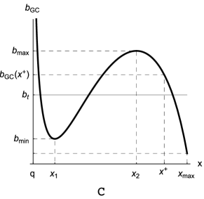
Figure 6: Four typical types of shapes of function $b_{GC}(x)$ in D0-D4 system. Diagram A/B/C/D correspond to region A/B/C/D in figure 5 respectively.

The first diagram of figure 6 corresponds to region A in the previous figure where $b_{GC}$ is shown to be monotonically decreasing. So, at any $\bar{b}>b_{2}$, the brane system is thermally stable. In addition, electrical stability condition requires $\bar{x}>x^{+}$ or, equivalently, $\bar{b}<b_{GC}(x^{+})$. Therefore the condition for the brane phase to be stable in region A is $b_{2}<\bar{b}<b_{GC}(x^{+})$.

In region B, C or D, $b_{GC}$ has two extremum points, the minimum at $x_{1}$ and the maximum at $x_{2}$. At these two points, we define their corresponding values of $b_{GC}$ as $b_{min}=b_{GC}(x_{1})$ and $b_{max}=b_{GC}(x_{2})$. This shape of $b_{GC}$ makes it possible to have two locally stable black brane phases, one with horizon size smaller than $x_{1}$ and the other larger than $x_{2}$. However, the electrical stability requires $x>x^{+}$ and the numerical computation shows that $x^{+}>x_{2}$ as shown in the first diagram in figure 7, which means that the smaller black brane phase is by no means electrically stable. So in the following analysis, we only need to find out whether the larger black brane phases are stable.

The difference between the $b_{GC}$ curves in region B, C and D is that in region B or C there exists a temperature $T_{t}=1/b_{t}$ at which the large black brane and the small one have the same thermodynamic potential whereas in region D, there is no such $b_{t}$ because the large black brane, if exists, always has higher thermodynamic potential than the smaller one under the same temperature. So in region D the larger black brane is globally unstable which means there exist no thermodynamicaly stable black brane phases in D, which is why we used a dotted line as the right boundary of region D in figure 5. The distinction between region B and C will be dealt with as follows.

Figure 7: The first diagram shows the numerical result of $x^{+}>x_{2}$ in region B, C and D. The second diagram shows a general relation between $b_{t}$ and $b_{GC}(x^{+})$ in region B and C though a special value $\Phi=0.5$ is chosen to plot this diagram.

On the one hand, since in both regions, for $\bar{b}\in(b_{2},b_{t})$ , the larger black brane always has lower free energy than the corresponding smaller black brane (if there is one), the thermal stability condition would be $b_{t}>\bar{b}>b_{2}$. On the other hand, since $x^{+}>x_{2}$, the electrical stability condition now becomes $b_{GC}(x^{+})>\bar{b}>b_{2}$. Combining these two conditions together, we get $b_{2}<\bar{b}<\textrm{min}\{b_{t},b_{GC}(x^{+})\}$. So we need to determine which one in $b_{t}$ and $b_{GC}(x^{+})$ is smaller. Again by numerical calculations, we find that there exists a charge $q_{0}\approx 0.1227$, above which (in region B) we have $b_{GC}(x^{+})<b_{t}$ and below which (in region C) we have $b_{GC}(x^{+})>b_{t}$, which is illustrated in the second diagram in figure 7. One may further notice that in figure 7, near (but less than) $q_{c}$ we have $b_{GC}(x^{+})<b_{t}$, which means that the state at the second order phase transition point is electrically unstable. So, we have finally shown that neither the second order nor the first order phase transition could happen in GC ensemble.

To summarize, the final stability condition can be stated as follows: the D0-D4 black brane can be a thermodynamically stable phase if

$$(\Phi,q)\in\textrm{A}\cup\textrm{B}\cup\textrm{C},\qquad b_{2}<\bar{b}<\left\{\begin{array}[]{ll}b_{GC}(x^{+}),&(\Phi,q)\in\textrm{A}\cup\textrm{B},\\ b_{t},&(\Phi,q)\in\textrm{C}\end{array}\right.,$$ (85)

otherwise there is no known stable phase.

5.3 CG ensemble

The CG ensemble analysis is similar, though more complicated, to that in GC ensemble. In fact, the symmetry of interchanging $(\Phi,q)$ and $(\varphi,Q)$ still exists after the electrical stability conditions are considered.

D2-D6-branes

By (71) and according to the thermal stability result, the constraint on $(\varphi,Q)$ is shown in figure 8 as region A whose right boundary is

$$Q=\frac{2(1-\varphi)^{2}(3\varphi-1)}{\varphi(3-5\varphi)}.$$ (86)

When $(\varphi,Q)\in\textrm{A}$, the shape of $b_{CG}(x)$ is shown in the second diagram of figure 8,

Figure 8: The first diagram shows the region in $Q$-$\varphi$ plane where the black brane can be stable and the second shows the shape of $b_{CG}$ in A.

and there exists a $b_{unstable}=b_{CG}(X)$ below which (and above $b_{2}$) the black brane phase has lowest thermodynamical potential. The critical value $X$ is defined as the solution to the following equation (please refer to appendix E in zhou:2015 for the detailed derivation),

$$f(X,Q,\varphi,p)\equiv\left(\frac{8-2p}{3-p}-Q\right)\sqrt{\xi}-\frac{(7-p)\xi}{2(3-p)}-\frac{3-\sqrt{(1-\xi)^{2}+4Q^{2}\xi}}{2}=0,\quad\textrm{for }p=2,$$ (87)

where $\xi=1-X+X\varphi^{2}$. One can numerically show that $x_{0}<X$ always holds, where $x_{0}$ is defined in (56). So for any $\bar{x}>X$, the black brane is automatically electrically stable. Therefore, the thermodynamic stability condition is

$$(\varphi,Q)\in\textrm{A}\quad\textrm{and}\quad b_{2}<\bar{b}<b_{unstable}.$$ (88)

D1-D5-branes

Similar to GC ensemble, the electrical and thermal stability condition restricts $(\varphi,Q)$ to the region shown in figure 9.

Figure 9: Regions in $Q$-$\varphi$ plane where there may exist a stable black brane phase.

The right boundary of region C in this figure is described by

$$Q=\frac{(2-\varphi)(2\varphi-1)}{3\varphi}.$$ (89)

In region A, $b_{CG}$ is monotonically decreasing and is depicted in the first diagram of figure 10. It is easy to see that the stability condition for $\bar{b}$ is $b_{2}<\bar{b}<b_{CG}(x_{0})$. In region B or C, $b_{CG}$ could look like the curves in the second or third diagrams depending on the values of $\varphi$ and $Q$ (actually only depending on $Q$ which will be demonstrated later).

Figure 10: Typical shapes of $b_{CG}(x)$ in D1-D5 system. Diagram A/B/C correspond to region A/B/C in figure 9 respectively.

In both cases, there exists a $b_{unstable}$ and only below it (and above $b_{2}$) the black brane can be thermally stable. Again $b_{unstable}=b_{CG}(X)$ where $X$ is the solution to $f(X,Q,\varphi,1)=0$. In $p=1$ case, this equation can be reduced to the following equation,

$$2\xi-(5-3Q)\sqrt{\xi}+2=0,$$ (90)

which has solution

$$\sqrt{\xi}=\frac{1}{4}\left(5-3Q-\sqrt{3(3-Q)(1-3Q)}\right).$$ (91)

Now we want to find the region where $X<x_{0}$ which is equivalent to $\sqrt{\xi}>1/\sqrt{2}$. This can be readily solved and gives $1/3>Q>5/3-\sqrt{2}$ which corresponds to region B in figure 9. This also proves in region C we have $X>x_{0}$.

Combining all cases together, we obtain the final condition for D1-D5-branes to be stable in CG ensemble,

$$(\varphi,Q)\in\textrm{A}\cup\textrm{B}\cup\textrm{C}\quad\textrm{and}\quad b_{2}<\bar{b}<\left\{\begin{array}[]{ll}b_{CG}(x_{0}),&(\varphi,Q)\in\textrm{A}\cup\textrm{B}\,,\\ b_{unstable},&(\varphi,Q)\in\textrm{C}\,.\end{array}\right.$$ (94)

D0-D4-branes

We have seen enough evidences that GC ensemble and CG ensemble are related to each other by the exchange of $\Phi\leftrightarrow\varphi$ and $Q\leftrightarrow q$, and it is not too hard to convince oneself that this is also true for D0-D4 branes by the same calculations as in previous subsections. So, we shall omit most of the rigorous deduction details and simply represent the final results below. The regions that can have both electrically and thermally stable black brane phases in $Q-\varphi$ plane are shown in figure 11.

Figure 11: Regions in $Q$-$\varphi$ plane where stable phases can exist. $Q_{c}$ and $Q_{0}$ respectively have the same values as $q_{c}$ and $q_{0}$ in GC ensemble, i.e. $Q_{c}\approx 0.1416$ and $Q_{0}\approx 0.1227$.

Figure 12: Typical shapes of $b_{CG}$ in D0-D4 system. Diagram A/B/C correspond to region A/B/C in figure 11 respectively.

As to the constraint on $\bar{b}$, in region A, $b_{CG}$ looks like the curve in the first diagram in figure 12, so in order for the system to be stable, we need $b_{2}<\bar{b}<b_{CG}(x_{0})$. In region B and C, $b_{CG}$ has the shape shown in the second and third diagrams respectively and in both regions there exists a $b_{t}$ which has the same meaning as the $b_{t}$ in figure 6. The difference between region B and C is that in the former we have $b_{t}>b_{CG}(x_{0})$ while in the latter otherwise. Hence in region B, we need $b_{2}<\bar{b}<b_{CG}(x_{0})$ while in region C we need $b_{2}<\bar{b}<b_{t}$. Thus the final stability condition,

$$(\varphi,Q)\in\textrm{A}\cup\textrm{B}\cup\textrm{C}\quad\textrm{and}\quad b_{2}<\bar{b}<\left\{\begin{array}[]{ll}b_{CG}(x_{0}),&(\varphi,Q)\in\textrm{A}\cup\textrm{B},\\ b_{t},&(\varphi,Q)\in\textrm{C}\end{array}\right..$$ (97)

Again we would like to point out that the first/second order van der Waals-like phase transition found by thermal stability computations can no long occur now due to the electrical instability.

5.4 CC ensemble

The thermal stability properties are gathered in the appendix A in our paper zhou:2015 . These properties, especially in the D1-D5 case, are originally investigated in lu:2012 . Now we can incorporate the thermal stability conditions there with the newly gained electrical stability condition in (73) to find the thermodynamic stability conditions.

D2-D6-branes

Again we shall start with D2-D6 system in which almost all results can be obtained analytically. In CC ensemble, the variable $b_{2}\equiv b(x_{max}=1)$ as defined in other ensembles is just as 0. So for any high enough temperature (or small enough $\bar{b}$) there always exists a stable (both thermally and electrically) black brane phase. However, for large $\bar{b}$ there can be very different phenomena depending on the shapes of $b_{CC}$ in different regions of $Q$-$q$ plane. In region A (as shown in figure 13), $b_{CC}$ is the curve shown in diagram A in figure 14.

Figure 13: Regions in the $Q$-$q$ plane where there exist different types of $b_{CC}$ curves.

Figure 14: Shapes of $b_{CC}$ of D2-D6 system. Diagram A/B/C correspond to region A/B/C in figure 13 respectively.

One can see that in this region, the electrical stability constraint on $\bar{b}$ is $0<\bar{b}<b_{CC}(x^{+})$, where

$$b_{CC}(x^{+})=\frac{1}{3\sqrt{3}}\sqrt{(1+\sqrt{1+3Q^{2}})(1+\sqrt{1+3q^{2}})}.$$ (98)

The shapes of $b_{CC}$ in region B and C are shown in the other two diagrams B and C respectively. In both B and C, there exists a $b_{unstable}$ that corresponds to the equality between the free energy of black brane and the state with $x=q$, and only below this $b_{unstable}$ the black brane is the global minimum of free energy. The difference between these two regions is that in region B, $b_{unstable}>b_{CC}(x^{+})$ while in region C it is otherwise, and this difference obviously leads to different constraints on $\bar{b}$. The line which divides region B and C and also on which $b_{unstable}=b_{CC}(x^{+})$ is described by following relation,

$$(\sqrt{1+3q^{2}}-\sqrt{3}q)+(\sqrt{1+3Q^{2}}-\sqrt{3}Q)=8-4\sqrt{3}.$$ (99)

There is also an interesting feature that the symmetry between D2 and D6 can be explicitly seen via the symmetry between $Q$ and $q$ in (98) and (99).

To sum up, the dynamical stability condition for D2-D6 system in CC ensemble can be expressed by the following simple constraint,

$$(0<)\ \bar{b}<\left\{\begin{array}[]{ll}b_{CC}(x^{+}),&(Q,q)\in\textrm{A}\cup\textrm{B},\\ b_{unstable},&(Q,q)\in\textrm{C}\end{array}\right..$$ (102)

D1-D5-branes

For D1-D5 system, the $Q-q$ plane can also be divided into three regions (see figure 15) and in each region the shape of $b_{CC}$ is shown in figure 16.

Figure 15: Regions in the $Q$-$q$ plane where there exist different types of $b_{CC}$ curves.

The two lines dividing region A, B and B, C can not be analytically solved and are both obtained numerically. With experiences of dealing with so many cases in previous analyses, we can easily read out the final stability condition from figure 16,

$$(0<)\ \bar{b}<\left\{\begin{array}[]{ll}b_{CC}(x^{+}),&(Q,q)\in\textrm{A}\cup\textrm{B},\\ b_{t},&(Q,q)\in\textrm{C}\end{array}\right..$$ (105)

Figure 16: Shapes of $b_{CC}$ of D1-D5 (or D0-D4) system in CC ensemble. Diagram A/B/C correspond to region A/B/C in figure 15 respectively.

D0-D4-branes

The D0-D4 system has very similar feature to the D1-D5 system except that the division of region A, B and C as shown in figure 17 is slightly different from figure 15.

Figure 17: Regions in the $Q$-$q$ plane where there exist different types of $b_{CC}$ curves. The constants are $q_{c}=Q_{c}\approx 0.1416$ and $q_{0}=Q_{0}\approx 0.1227$.

The shapes of $b_{CC}$ in each region resemble those in figure 16. Therefore, the final stability condition in terms of $\bar{b}$ is exact the same as the condition in (105), though the specific values of $b_{CC}(x^{+})$ and $b_{t}$ are different in general. One final remark is, in both D0-D4 and D1-D5 systems, the first order and second order phase transitions would not arise any more because of the instability of the small black brane phase in the first order phase transition and of the state at the critical point in the second order phase transition.

5.5 Compatibilities

Finally, we should check the compatibility of results obtained from different ensembles. For example, if we take the limit $Q\to 0$ in CC ensemble, or we take the limit $\Phi\to 0$ in GC ensemble, in both limits we would end up with a canonical ensemble for D$(p+4)$-branes. Hence compatibility requires the stability conditions in these two ensembles should degenerate into the same condition at the aforementioned limits. This can be easily seen by noticing the following two facts. First, from (8) we can see that $b(x,Q=0,q)=b(x,\Phi=0,q)$ which means the thermal stability conditions coincides in these two limits. Second, by setting $\Phi\to 0$, one realizes that in GC ensemble $x_{max}\to 1$, so the two electrical stability conditions in (72) and (73) degenerate. Therefore, we proved the thermodynamic stability conditions in CC and GC ensembles are compatible. Similarly, one can also easily check the other compatibilities such as the degeneracy of CC and CG ensembles in the limit of $q\to 0$ and $\varphi\to 0$, the degeneracy of GG and GC in the same limit and so on. So, the conclusion is, the stability conditions in all ensembles are compatible with each other.

6 Conclusions

In this paper and our previous paper zhou:2015 , we have conducted an exhaustive scan over the thermal and electrical stabilities of D$p$-D$(p+4)$-brane systems in all possible ensembles, and this paper is especially focusing on the electrical stabilities.

We have confirmed in GG ensemble the thermal stability alone already guarantees the thermodynamic stability which was found in lu:2011-2 for D$p$-brane systems. We find that in CG,GC and CC ensembles, the electrical stability conditions generate extra constraints on the horizon sizes and also on electric potentials only in GC and CG ensembles, besides the constraints that we already got from thermal stability conditions. These new conditions rule out the small brane phases from the old phase diagrams gained from pure thermal stability considerations. Consequently, for all possible $p$, there is no van der Waals-like phase structure any more, i.e. neither the first order small-large black brane transitions nor the second order phase transition. In the $Q\to 0$ limit, the electrical stability conditions also modify the one-charge brane system discussed in lu:2011 such that the van der Waals phase structures are invisible. Although we find this result in D$p$-D$(p+4)$-brane systems, we expect that it may be a common feature in other charged black hole systems. In fact, this electrical instability has already been noticed in EMadS black hole system studied in chamblin:1999-2 in which the black holes with smaller horizons near the van der Waals phase transition points were found to be unstable and hence the transition does not exist after the electrical instability is considered. Whether this is also the case for other systems could be left for future research works.

From the new phase diagrams, we find that the symmetry of interchanging $Q\leftrightarrow q$ and $\Phi\leftrightarrow\varphi$ is still kept after electrical stability conditions are considered. This symmetry in fact could be a result of the T-duality: If we make T-duality in the $p+1,\dots,p+4$ directions of the D$(p+4)$ brane in which the D$p$-charges are smeared, these two kinds of branes interchange with each other, which is equivalent to make above interchange in charges. This provides a natural interpretation of this symmetry of the phase structure.

Now, we have included the thermal stability and the electrical stability in the discussion of the thermodynamic structure of the black brane system. However, there are another two independent parameters, the volume of the cavity and the volume of the brane. The corresponding generalized forces are the pressures on the cavity or in the brane directions. These parameters may also introduce new stability conditions such as the compressibilities in different directions. This is in analogy to the similar discussions in AdS black holes or asymptotically AdS black holes in which the cosmological constant plays the role of the pressure Kastor:2009wy and the positivity of the compressibility also determines the stability of the systemDolan:2014lea . To discuss the effects of this kind of instability on the phase structure of the black brane system could also be a future research direction.

References

- (1) Jacob D. Bekenstein, Black holes and entropy, Phys. Rev. D 7, 2333 (1973).
- (2) S. W. Hawking, Particle creation by black holes, Commun. math. Phys. 43 199-220 (1975).
- (3) Gary T. Horowitz and Andrew Stromiger, Black strings and P-branes, Nucl. Phys. B 360 (1991) 197-209.
- (4) S. S. Gubser, I. R. Klebanov, and A. W. Peet, Entropy and temperature of black 3-branes, Phys. Rev. D 54, 3915 (1996), [arXiv:hep-th/9602135].
- (5) J. M. Bardeen, B. Carter, and S. W. Hawking, The four laws of black hole mechanics, Commun. math. Phys. 31 161-170 (1973).
- (6) G. W. Gibbons and S. W. Hawking, Action integrals and partition functions in quantum gravity, Phys. Rev. D 15, 2752 (1977).
- (7) S. W. Hawking and Don N. Page, Thermodynamics of black holes in anti-de Sitter space, Commun. math. Phys. 87 577-588 (1983).
- (8) James W. York, Jr., Black-hole thermodynamics and the Euclidean Einstein action, Phys. Rev. D 33, 2092 (1986).
- (9) Bernard F. Whiting and James W. York, Jr., Action Principle and Partition Function for the Gravitational Field in Black-Hole Topologies, Phys. Rev. Lett. 61, 1336 (1988).
- (10) H. W. Braden, J. D. Brown, B. F. Whiting and J. W. York, Charged black hole in a grand canonical ensemble, Phys. Rev. D 42, 3376 (1990).
- (11) Andrew Chamblin, et al., Charged AdS Black Holes and Catastrophic Holography, Phys. Rev. D 60, 064018 (1999), [arXiv:hep-th/9902170].
- (12) Andrew Chamblin, et al., Holography, thermodynamics, and fluctuations of charged AdS black holes, Phys. Rev. D 60, 104026 (1999), [arXiv:hep-th/9904197].
- (13) S. Carlip and S. Vaidya, Phase Transitions and Critical Behavior for Charged Black Holes, Class. Quant. Grav. 20 (2003) 3827-3838, [arXiv:gr-qc/0306054].
- (14) Andrew P. Lundgren, Charged black hole in a canonical ensemble, Phys. Rev. D 77, 044014 (2008), [arXiv:gr-qc/0612119].
- (15) Rabin Banerjee, Dibakar Roychowdhury, Thermodynamics of phase transition in higher dimensional AdS black holes, JHEP 11 (2011) 004, [arXiv:1109.2433].
- (16) Rabin Banerjee, Sujoy Kumar Modak, Dibakar Roychowdhury, A unified picture of phase transition: from liquid-vapour systems to AdS black holes, JHEP 10 (2012) 125, [arXiv:1106.3877].
- (17) Marco M. Caldarelli, Guido Cognola, and Dietmar Klemm, Thermodynamics of Kerr-Newman-AdS Black Holes and Conformal Field Theories, Class. Quant. Grav. 17 (2000) 399-420, [arXiv:hep-th/9908022].
- (18) Rong-Gen Cai, Gauss-Bonnet black holes in AdS spaces, Phys. Rev. D 65, 084014 (2002), [arXiv:hep-th/0109133].
- (19) Rong-Gen Cai, Sang Pyo Kim, and Bin Wang, Ricci flat black holes and Hawking-Page phase transition in Gauss-Bonnet gravity and dilaton gravity, Phys. Rev. D 76, 024011 (2007), [arXiv:0705.2469].
- (20) E. Witten, Instability of the Kaluza-Klein vacuum, Nucl. Phys. B 195 (1982) 481.
- (21) R. Gregory and R. Laflamme, Black strings and p-branes are unstable, Phys. Rev. Lett. 70 (1993) 2837. [hep-th/9301052].
- (22) R. Emparan and M. Martinez, Black Branes in a Box: Hydrodynamics, Stability, and Criticality, JHEP 1207 (2012) 120, [arXiv:1205.5646 [hep-th]].
- (23) J. X. Lu, Shibaji Roy, and Zhiguang Xiao, Phase transitions and critical behavior of black branes in canonical ensemble, JHEP 01 (2011) 133, [arXiv:1010.2068[hep-th]].
- (24) J. X. Lu, Shibaji Roy, and Zhiguang Xiao, The enriched phase structure of black branes in canonical ensemble, Nucl. Phys. B 854 (2012) 913, [arXiv:1105.6323[hep-th]].
- (25) J. X. Lu, Shibaji Roy, and Zhiguang Xiao, Phase structure of black branes in grand canonical ensemble, JHEP 05 (2011) 091, [arXiv:1011.5198[hep-th]].
- (26) Chao Wu, Zhiguang Xiao, and Jianfei Xu, Bubbles and Black Branes in Grand Canonical Ensemble, Phys. Rev. D 85, 044009 (2012), [arXiv:1108.1347[hep-th]].
- (27) Da Zhou and Zhiguang Xiao, Phase structures of the black D-D-brane system in various ensembles, [arXiv:1502.00261[hep-th]].
- (28) J. X. Lu, Ran Wei, and Jianfei Xu, The phase structure of black D1/D5 (F/NS5) system in canonical ensemble, JHEP 12 (2012) 012, [arXiv:1210.0708[hep-th]].
- (29) D. Kastor, S. Ray and J. Traschen, Enthalpy and the Mechanics of AdS Black Holes, Class. Quant. Grav. 26 (2009) 195011, [arXiv:0904.2765 [hep-th]].
- (30) B. P. Dolan, Thermodynamic stability of asymptotically anti-de Sitter rotating black holes in higher dimensions, Class. Quant. Grav. 31 (2014) 165011, [arXiv:1403.1507 [gr-qc]].