Parameterless stopping criteria for
recursive density matrix expansions

Abstract

Parameterless stopping criteria for recursive polynomial expansions to construct the density matrix in electronic structure calculations are proposed. Based on convergence order estimation the new stopping criteria automatically and accurately detect when the calculation is dominated by numerical errors and continued iteration does not improve the result. Difficulties in selecting a stopping tolerance and appropriately balancing it in relation to parameters controlling the numerical accuracy are avoided. Thus, our parameterless stopping criteria stand in contrast to the standard approach to stop as soon as some error measure goes below a user-defined parameter or tolerance. We demonstrate that the stopping criteria work well both in dense and sparse matrix calculations and in large-scale self-consistent field calculations with the quantum chemistry program Ergo (www.ergoscf.org).

1 Introduction

An important computational task in electronic structure calculations based on for example Hartree–Fock ¹ or Kohn–Sham density functional theory ^{2, 3} is the computation of the one-electron density matrix $D$ for a given Fock or Kohn–Sham matrix $F$. The density matrix is the matrix for orthogonal projection onto the subspace spanned by eigenvectors of $F$ that correspond to occupied electron orbitals:

$$Fx_{i} =\lambda_{i}x_{i},$$ (1.1)

$$D\coloneqq \sum_{i=1}^{n_{\textrm{occ}}}x_{i}x_{i}^{T},$$ (1.2)

where the eigenvalues of $F$ are arranged in ascending order

$$\lambda_{1}\leq\lambda_{2}\leq\dots\leq\lambda_{\textrm{homo}}<\lambda_{\textrm{lumo}}\leq\dots\leq\lambda_{N-1}\leq\lambda_{N},$$ (1.3)

$n_{\textrm{occ}}$ is the number of occupied orbitals, $\lambda_{\textrm{homo}}$ is the highest occupied molecular orbital (homo) eigenvalue, and $\lambda_{\textrm{lumo}}$ is the lowest unoccupied molecular orbital (lumo) eigenvalue and where we assume that there is a gap

$$\xi\coloneqq\lambda_{\textrm{lumo}}-\lambda_{\textrm{homo}}>0$$ (1.4)

between eigenvalues corresponding to occupied and unoccupied orbitals. An essentially direct method to compute $D$ is to compute an eigendecomposition of $F$ and assemble $D$ according to (1.2). Unfortunately, the computational cost of this approach increases cubically with system size which limits applications to rather small systems. Alternative methods have therefore been developed with the aim to reduce the computational complexity ⁴. One approach is to view the problem as a matrix function

$$D=\theta(\mu I-F),$$ (1.5)

where $\theta$ is the Heaviside function and $\mu$ is located between $\lambda_{\textrm{homo}}$ and $\lambda_{\textrm{lumo}}$, which makes (1.5) equivalent to the definition in (1.2) ⁵. A condition number for the problem of evaluating (1.5) is given by

$$\kappa\coloneqq\lim_{h\rightarrow 0}\sup_{A:\|A\|=\Delta\epsilon}\frac{\|\theta(\mu I-(F+hA))-\theta(\mu I-F)\|}{h}=\frac{\Delta\epsilon}{\xi}$$ (1.6)

where $\Delta\epsilon$ is the spectral width of $F$ ^{6, 7, 8}. We let $\|A\|=\Delta\epsilon$ to make the condition number invariant both to scaling and shift of the eigenspectrum of $F$ ⁷.

When the homo-lumo gap $\xi>0$, a function that varies smoothly between 0 and 1 in the gap can be used in place of (1.5). To construct such a function, recursive polynomial expansions or density matrix purification have proven to be particularly simple and efficient ⁹.

Algorithm 1 Recursive polynomial expansion (general form)

1:$X_{0}=f_{0}(F)$

2:$\widetilde{X}_{0}=X_{0}+E_{0}$

3:while stopping criterion not fulfilled, for $i=1,2,\dots$ do

4:     $X_{i}=f_{i}(\widetilde{X}_{i-1})$

5:     $\widetilde{X}_{i}=X_{i}+E_{i}$

6:end while

The regularized step function is built up by the recursive application of low-order polynomials $f_{0},f_{1},\dots$, see Algorithm 1. With this approach, a linear scaling computational cost is achieved provided that the matrices in the recursive expansion are sufficiently sparse, which is usually ensured by removing small matrix elements during the course of the recursive expansion ¹⁰. In Algorithm 1 the removal of matrix elements, also called truncation, is written as an explicit perturbation $E_{i}$ added to the matrix in each iteration. Several recursive expansion algorithms fitting into the general form of Algorithm 1 have been proposed. Note that here we are considering methods that operate in orthogonal basis. The function $f_{0}$ is usually a first order polynomial that moves all eigenvalues into the $[0,\ 1]$ interval in reverse order. A natural choice for the iteration function $f_{i},\ i=1,2,\dots$ is the McWeeny polynomial $3x^{2}-2x^{3}$ ^{11, 12}, which makes Algorithm 1 essentially equivalent to the Newton–Schulz iteration for sign matrix evaluation ⁶. Furthermore, algorithms were developed that do not require beforehand knowledge of $\mu$. Palser and Manolopoulos proposed a recursive expansion based on the McWeeny polynomial ¹². Niklasson proposed a simple and efficient algorithm based on the second order polynomials $x^{2}$ and $2x-x^{2}$ ¹³. We will refer to this algorithm as the SP2 algorithm. The recursive application of polynomials gives a rapid increase of the polynomial order and the computational cost increases only with the logarithm of the condition number ^{13, 9}. The computational cost can be further reduced by a scale-and-fold acceleration technique giving an even weaker dependence on the condition number ¹⁴. Recursive expansion algorithms are key components in a number of linear scaling electronic structure codes including CP2K ¹⁵, Ergo ^{16, 17}, FreeON ¹⁸, Honpas ¹⁹, and LATTE ²⁰. Since most of the computational work lies in matrix-matrix multiplications, recursive expansion algorithms are well suited for parallel implementations ^{21, 22, 23, 24} and a competitive alternative to diagonalization also in the dense matrix case ^{22, 23}.

Different ways to decide when to stop the iterations have been suggested. A common approach is to stop when some quantity, measuring how far the matrix is from idempotency, goes below a predetermined convergence threshold value. The deviation from idempotency has been measured by the trace ^{25, 24} or some matrix norm ^{23, 6, 26, 27, 28, 15} of $X_{i}-X_{i}^{2}$ sometimes scaled by for example the matrix dimension. However, since the recursive expansion is at least quadratically convergent, what one usually wants is to continue iterating until the idempotency error does not anymore decrease substantially. This happens when any further substantial decrease is prevented by rounding errors or errors due to removal of matrix elements.

To find a proper relation between matrix element removal and the parameter measuring idempotency can be a delicate task, often left to the user of the routine. However, a few attempts to automatically detect when numerical errors start to dominate exist in the literature. Palser and Manolopoulos noted that with their expansions, the functional $\textrm{Tr}[X_{i}F]$ decreases monotonically in exact arithmetics and suggested to stop on its first increase which should be an indication of stagnation ¹². A similar criterion for the SP2 expansion was proposed by Cawkwell et al. ²². In this case, the iterations are stopped on an increase of the idempotency error measure $|\textrm{Tr}[X_{i}-X_{i}^{2}]|$. However, the value of the functional or the idempotency error may continue to decrease without significant improvement of the accuracy. In such cases, the computational effort in last iterations is no longer justified. In the present work, we propose new parameterless stopping criteria based on convergence order estimation. The stopping criteria are general and can be used both in the dense and sparse matrix cases using different strategies for truncation, and with different choices of polynomials.

2 Parameterless stopping criteria

The iterations of density matrix expansions can be divided into three phases ^{29, 30}: 1) the conditioning phase where the deviation from idempotency decreases less than quadratically or not at all, 2) the purification phase where the idempotency error decreases at least quadratically, and 3) the stagnation phase where the idempotency error again does not decrease significantly or at all, see Figure 2.1.

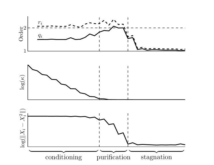
Figure 2.1: Illustration of the three phases for a recursive expansion of order $q=2$ based on the polynomials $x^{2}$ and $2x-x^{2}$ (see Section 4). In the conditioning phase the matrix does not come closer to idempotency but the condition number, $\kappa$, is lowered. In the purification phase the condition number is close to 1 and idempotency is approached quadratically. In the stagnation phase numerical errors start to dominate and the matrix again does not come closer to idempotency. The upper panel shows what we call the observed orders of convergence $q_{i}$ and $r_{i}$. Throughout the conditioning and purification phases $r_{i}\geq 2$ but in the stagnation phase $r_{i}<2$.

Here, we propose new parameterless stopping criteria designed to automatically and accurately detect the transition between purification and stagnation, so that the procedure can be stopped without superfluous iterations in the stagnation phase. We measure the deviation from idempotency by

$$e_{i}\coloneqq\|X_{i}-X_{i}^{2}\|_{2}.$$ (2.1)

We recall that an iterative method has asymptotic order of convergence $q$ if it in exact arithmetics generates a sequence of errors $e_{1},e_{2},\dots$ such that

$$\lim_{i\rightarrow\infty}\frac{e_{i}}{e_{i-1}^{q}}=C^{\infty},$$ (2.2)

where $C^{\infty}$ is an asymptotic constant. The order of convergence can also be observed numerically by

$$q\approx\frac{\log(e_{i}/C^{\infty})}{\log(e_{i-1})}\eqqcolon q_{i}.$$ (2.3)

Our stopping criteria are based on the detection of a discrepancy between the asymptotic and observed orders of convergence. When the stagnation phase is entered numerical errors start to dominate, leading to a fall in the observed order of convergence, see the upper panel in Figure 2.1.

Since the observed order can be significantly smaller than the asymptotic order also in the initial conditioning phase, an issue is how to determine when the purification phase has started and one can start to look for a drop in the order $q_{i}$. A similar problem of determining the iteration when to start to check the stopping criterion appears in the method described by Cawkwell et al. ²². Our solution is to replace the asymptotic constant $C^{\infty}$ in (2.3) with a larger value such that the observed order of convergence in exact arithmetics is always larger than or equal to the asymptotic order of convergence. In other words we want to find $C_{q}$, as small as possible, such that in exact arithmetics

$$r_{i}\coloneqq\frac{\log(e_{i}/C_{q})}{\log(e_{i-1})}\geq q$$ (2.4)

for all $i$. One may let $C_{q}$ vary over the iterations but we will later see that it is usually sufficient to use a single value $C_{q}$ for the whole expansion. Important is that, in exact arithmetics, $r_{i}\geq q$ for all $i$. In the presence of numerical errors $r_{i}$ is significantly smaller than $q$ only in the stagnation phase. We may therefore start to look for a drop in $r_{i}$ immediately. As soon as the observed order of convergence, $r_{i}$, goes significantly below $q$, the procedure should be stopped, since this indicates the transition between purification and stagnation. In this way we avoid the issue of detecting the transition between conditioning and purification. See the upper panel in Figure 2.1 for an illustration.

For clarity we note that (2.4) is equivalent to

$$C_{q}\geq\frac{e_{i}}{e_{i-1}^{q}}=\frac{\|f_{i}(X_{i-1})-f_{i}(X_{i-1})^{2}\|_{2}}{\|X_{i-1}-X_{i-1}^{2}\|_{2}^{q}}.$$ (2.5)

For generality and simplicity we want to assume as little information as possible about the eigenspectra of $X_{i},\ i=0,1,\dots$. We will use the following theorem to find the smallest possible $C_{q}$ value fulfilling (2.5) with no or few assumptions about the location of eigenvalues for several recursive expansion polynomials of interest for appropriate choices of $q$.

Theorem 1.

Let $f$ be a continuous function from $[0,\ 1]$ to $[0,\ 1]$ and assume that the limits

$$\lim_{x\rightarrow a^{+}}\frac{f(x)-f(x)^{2}}{(x-x^{2})^{q}}\quad\text{and}\quad\lim_{x\rightarrow(1-a)^{-}}\frac{f(x)-f(x)^{2}}{(x-x^{2})^{q}}$$ (2.6)

exist for some $q>0$, where $a\in[0,\ 0.5]$. Let $H$ denote the set of Hermitian matrices with all eigenvalues in $[0,\ 1]$ and at least one eigenvalue in $[a,\ 1-a]$. Then,

$$\max_{X\in H}\frac{\|f(X)-f(X)^{2}\|_{2}}{\|X-X^{2}\|_{2}^{q}}=\max_{x\in[0,1]}g(x,a),$$ (2.7)

where

$$g(x,a)\coloneqq\left\{\begin{array}[]{ll}\frac{f(x)-f(x)^{2}}{(x-x^{2})^{q}}&\textrm{if }a\leq x\leq 1-a,\\ \frac{f(x)-f(x)^{2}}{(a-a^{2})^{q}}&\textrm{otherwise,}\end{array}\right.$$ (2.8)

is extended by continuity at $x=0$ and $x=1$ for $a=0$.

As suggested by Theorem 1, we will choose $C_{q}\coloneqq\max_{x\in[0,1]}g(x,a)$ thereby making sure that (2.5) is fulfilled. In principle, the value $a$ should be chosen as large as possible to get the smallest possible $C_{q}$-value, since a larger $a$ gives a smaller set of matrices $H$ in (2.7). We note that it is possible to let $C_{q}$ vary by choosing the largest possible $a$ in every iteration, but in this work we will attempt to use a single value for the whole expansion whenever possible. There is always at least one eigenvalue in the interval $[0,\ 1]$ in every iteration. Therefore, if, for the given recursive expansion polynomials $f_{i}$, the limits (2.6) exist with $a=0$ we employ the theorem with $a=0$. Only if the limits (2.6) do not exist with $a=0$ will we use the theorem with $a>0$ and in general get different values of $C_{q}$ in every iteration. In such a case some information about the eigenspectrum of $X_{i}$ in each iteration $i$ is needed so that $a$ can be chosen appropriately. The theorem should be invoked with $q$ equal to the order of convergence of the recursive expansion.

Proof of Theorem 1.

Continuity of $f(x)$ together with existence of the two limits (2.6) (needed in case $a=0$) implies existence of $\max_{x\in[0,1]}g(x,a)$. Let $X$ be a matrix in $H$. Then,

$$\frac{\|f(X)-f(X)^{2}\|_{2}}{\|X-X^{2}\|_{2}^{q}}\leq \max_{x\in[0,1]}\max_{\begin{subarray}{c}y\in[a,1-a]\\ |y-0.5|\leq|x-0.5|\end{subarray}}\frac{f(x)-f(x)^{2}}{(y-y^{2})^{q}}$$ (2.9)

$$= \max\left(\max_{x\in[a,1-a]}\max_{|y-0.5|\leq|x-0.5|}\frac{f(x)-f(x)^{2}}{(y-y^{2})^{q}},\right.$$ (2.10)

$$\phantom{\max\left(\right.}\left.\max_{x\in[0,1]\setminus[a,1-a]}\max_{y\in[a,1-a]}\frac{f(x)-f(x)^{2}}{(y-y^{2})^{q}}\right)$$

$$= \max\left(\max_{x\in[a,1-a]}\frac{f(x)-f(x)^{2}}{(x-x^{2})^{q}},\right.$$ (2.11)

$$\phantom{\max\left(\right.}\left.\max_{x\in[0,1]\setminus[a,1-a]}\frac{f(x)-f(x)^{2}}{(a-a^{2})^{q}}\right)$$

$$= \max_{x\in[0,1]}g(x,a).$$ (2.12)

The maximum in (2.7) is attained for any matrix in $H$ with an eigenvalue $\lambda=\operatorname*{arg\,max}_{x\in[0,1]}g(x,a)$. ∎

Remark 2.1.

Inequality (2.9) can be interpreted as follows. The arguments of the maxima, $x$ and $y$, play the roles of the eigenvalues of $X$ that define $\|f(X)-f(X)^{2}\|_{2}$ and $\|X-X^{2}\|_{2}$, respectively. While, for all we know, $x$ can be any eigenvalue, $y$ is necessarily the eigenvalue of $X$ that is closest to 0.5. In other words,

$$y=\operatorname*{arg\,min}_{\lambda\in\{\lambda_{i}\}}|\lambda-0.5|$$ (2.13)

and

$$\|X-X^{2}\|_{2}=\max_{\lambda\in\{\lambda_{i}\}}\lambda-\lambda^{2}=y-y^{2},$$ (2.14)

where $\{\lambda_{i}\}$ are the eigenvalues of $X$. Since there is at least one eigenvalue at $x$ and at least one eigenvalue in $[a,\ 1-a]$ the constraints on $y$ in (2.9) follow.

By construction, the observed convergence order $r_{i}$ may in exact arithmetics end up exactly equal to $q$. We want to detect when numerical errors start to dominate and $r_{i}$ drops significantly below $q$ but at the same time we want to disregard small perturbations that cause $r_{i}$ to go only slightly below $q$. In practice we will therefore use a parameter $\tilde{q}<q$ in place of $q$. In other words, our stopping criteria will be on the form stop as soon as $\log(e_{i}/C_{q})/\log(e_{i-1})<\tilde{q}$. In this work we will mainly consider second order expansions with $q=2$ and will then use $\tilde{q}=1.8$.

The spectral norm is often expensive to compute and one may therefore want to use an estimate in its place. One cheap alternative is the Frobenius norm

$$v_{i}\coloneqq\|X_{i}-X_{i}^{2}\|_{F}=\sqrt{\sum_{j}\left(\lambda_{j}-\lambda_{j}^{2}\right)^{2}},$$ (2.15)

where $\{\lambda_{j}\}$ are the eigenvalues of $X_{i}$. We expect the Frobenius norm to be a good estimate to the spectral norm when we are close to convergence since then many eigenvalues are clustered around 0 and 1 and do not contribute significantly to the sum in (2.15). Since $\|X_{i}-X_{i}^{2}\|_{2}\leq\|X_{i}-X_{i}^{2}\|_{F}$ we have that

$$v_{i}=K_{i}e_{i}$$ (2.16)

for some $K_{i}\geq 1$. Assume that for a given $q$

$$K_{i}\leq K_{i-1}^{q}.$$ (2.17)

Then,

$$v_{i}=K_{i}e_{i}\leq K_{i-1}^{q}C_{q}e_{i-1}^{q}=C_{q}v_{i-1}^{q},$$ (2.18)

and, assuming that $v_{i-1}<1$,

$$\frac{\log(v_{i}/C_{q})}{\log(v_{i-1})}\geq q,$$ (2.19)

which means that if the assumptions above hold we will not stop prematurely. In the following sections we will see under what conditions (2.17) holds for specific choices of polynomials for the recursive expansion.

For very large systems, it may happen that $v_{i}$ never goes below 1 because of the large number of eigenvalues that contribute to the sum in (2.15), in such a case the stopping criterion in the suggested above form will not be checked. One may then make use of the so-called mixed norm ³¹. Let the matrix be divided into square submatrices of equal size, padding the matrix with zeros if needed. One can define the mixed norm as the spectral norm of a matrix with elements equal to the Frobenius norms of the obtained submatrices. It can be shown that

$$e_{i}\leq m_{i}\leq v_{i}$$ (2.20)

where $m_{i}\coloneqq\|X_{i}-X_{i}^{2}\|_{M}$ is the mixed norm of $X_{i}-X_{i}^{2}$ in iteration $i$. The result for the Frobenius norm above that we will not stop prematurely therefore holds also for the mixed norm under the corresponding assumptions, i.e. (2.16) and (2.17) with $v_{i}$ replaced by $m_{i}$ and $m_{i-1}<1$. However, with a fixed submatrix block size the asymptotic behavior of the mixed norm follows that of the spectral norm. Thus, the quality of the stopping criterion will not deteriorate with increasing system size. One may therefore consider using the mixed norm for large systems.

We will in the following mainly focus on the regular and accelerated McWeeny and second order spectral projection polynomials.

3 McWeeny polynomial

We will first consider a recursive polynomial expansion based on the McWeeny polynomial $p_{\mathrm{mw}}(x)\coloneqq 3x^{2}-2x^{3}$ ^{11, 12}, i.e. Algorithm 1 with

$$\left\{\begin{aligned} f_{0}(x)&=\displaystyle\frac{\mu-x}{2\max(\lambda_{\textrm{max}}-\mu,\mu-\lambda_{\textrm{min}})}+0.5,\quad\\ f_{i}(x)&=p_{\textrm{mw}}(x),\quad i=1,2,\dots.\end{aligned}\right.$$ (3.1)

Here, $\lambda_{\textrm{min}}$ and $\lambda_{\textrm{max}}$ are the extremal eigenvalues of $F$ or bounds thereof, i.e.

$$\lambda_{\textrm{min}}\leq\lambda_{1}\textrm{ and }\lambda_{\textrm{max}}\geq\lambda_{N}.$$ (3.2)

We want to find the smallest value $C_{2}^{\textrm{mw}}$ such that

$$\frac{\log(e_{i}/C_{2}^{\textrm{mw}})}{\log(e_{i-1})}\geq 2$$ (3.3)

in exact arithmetics. Note that

$$\lim_{x\rightarrow 0^{+}}\frac{p_{\textrm{mw}}(x)-p_{\textrm{mw}}(x)^{2}}{(x-x^{2})^{2}}=\lim_{x\rightarrow 1^{-}}\frac{p_{\textrm{mw}}(x)-p_{\textrm{mw}}(x)^{2}}{(x-x^{2})^{2}}=3.$$ (3.4)

Thus, we may invoke Theorem 1 with $f=p_{\textrm{mw}}$, $a=0$ and $q=2$ which gives

$$C_{2}^{\textrm{mw}}=\max_{x\in[0,1]}\frac{p_{\textrm{mw}}(x)-p_{\textrm{mw}}(x)^{2}}{(x-x^{2})^{2}}=\max_{x\in[0,1]}(3+4x-4x^{2})=4$$ (3.5)

and we suggest to stop the expansion as soon as

$$\frac{\log(e_{i}/4)}{\log(e_{i-1})}<1.8.$$ (3.6)

We note that the McWeeny polynomial can be defined as the polynomial with fixed points at 0 and 1 and one vanishing derivative at 0 and 1. For polynomials with fixed points at 0 and 1 and $q-1$ vanishing derivatives at 0 and 1, sometimes referred to as the Holas polynomials ³², it can be shown that the smallest value $C_{q}^{\textrm{h}}$ such that

$$\frac{\log(e_{i}/C_{q}^{\textrm{h}})}{\log(e_{i-1})}\geq q$$ (3.7)

is $C_{q}^{\textrm{h}}=4^{q-1}$.

3.1 Acceleration

Prior knowledge of the homo and lumo eigenvalues makes it possible to use a scale-and-fold technique to accelerate convergence ¹⁴. In each iteration the eigenspectrum is stretched out so that the projection polynomial folds the eigenspectrum over itself. This technique is quite general and may be applied to a number of recursive expansions making use of various polynomials. In case of the McWeeny polynomial the eigenspectrum is stretched out around 0.5, see Algorithm 2. The amount of stretching is determined by the parameter $\tilde{\xi}$ which is an estimate of the homo-lumo gap $\xi$ such that at least one eigenvalue of $F$ is in $[\mu-\tilde{\xi}/2,\ \mu+\tilde{\xi}/2]$. With $\alpha=1$ on line 8, Algorithm 2 reduces to the regular McWeeny expansion discussed above.

Algorithm 2 McW-ACC algorithm

1:input: $F$, $\lambda_{\textrm{min}}$, $\lambda_{\textrm{max}}$, $\mu$, $\tilde{\xi}$

2:$\gamma=2\max(\lambda_{\textrm{max}}-\mu,\mu-\lambda_{\textrm{min}})$

3:$\beta_{0}=0.5(1-\tilde{\xi}/\gamma)$

4:$X_{0}=\frac{\mu I-F}{\gamma}+0.5I$

5:$\widetilde{X}_{0}=X_{0}+E_{0}$

6:$e_{0}=\|\widetilde{X}_{0}-\widetilde{X}_{0}^{2}\|_{2}$

7:for $i=1,2,\dots$ do

8:     $\alpha=3/(12\beta_{i-1}^{2}-18\beta_{i-1}+9)^{1/2}$

9:     $X_{s}=\alpha(\widetilde{X}_{i-1}-0.5I)+0.5I$

10:     $X_{i}=3X_{s}^{2}-2X_{s}^{3}$

11:     $\beta_{s}=\alpha(\beta_{i-1}-0.5)+0.5$

12:     $\beta_{i}=3\beta_{s}^{2}-2\beta_{s}^{3}$

13:     $\widetilde{X}_{i}=X_{i}+E_{i}$

14:     $e_{i}=\|\widetilde{X}_{i}-\widetilde{X}_{i}^{2}\|_{2}$

15:     if $\frac{\log(e_{i}/4)}{\log(e_{i-1})}<1.8$ then

16:         $n=i$

17:         break

18:     end if

19:end for

20:output: $n$, $\widetilde{X}_{n}$

As for the regular McWeeny expansion we want to find the smallest value $C_{2}^{\textrm{mwa}}$ such that

$$\frac{\log(e_{i}/C_{2}^{\textrm{mwa}})}{\log(e_{i-1})}\geq 2.$$ (3.8)

For the sake of analysis we introduce

$$p_{\textrm{mwa}}(x,\beta) \coloneqq p_{\textrm{mw}}\left(3(12\beta^{2}-18\beta+9)^{-1/2}(x-0.5)+0.5\right).$$ (3.9)

Note that line 10 in Algorithm 2 is equivalent to $X_{i}=p_{\textrm{mwa}}(\widetilde{X}_{i-1},\beta_{i-1})$. Furthermore, let

$$g(x,\beta)=\begin{dcases}g_{1}(x,\beta)&\textrm{if }x\in[\beta,\ 1-\beta],\\ g_{2}(x,\beta)&\textrm{otherwise,}\end{dcases}$$ (3.10)

where

$$g_{1}(x,\beta) =\frac{p_{\textrm{mwa}}(x,\beta)-p_{\textrm{mwa}}(x,\beta)^{2}}{(x-x^{2})^{2}},$$ (3.11)

$$g_{2}(x,\beta) =\frac{p_{\textrm{mwa}}(x,\beta)-p_{\textrm{mwa}}(x,\beta)^{2}}{(\beta-\beta^{2})^{2}},$$ (3.12)

which are plotted in Figure 3.1 for $\beta=0.3$.

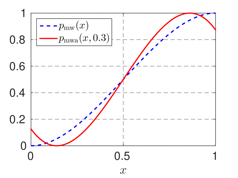
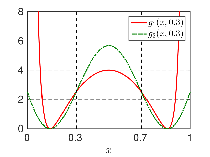
Figure 3.1: The left panel shows the regular $p_{\textrm{mw}}(x)$ and accelerated $p_{\textrm{mwa}}(x,\beta)$ McWeeny polynomials with $\beta=0.3$. The right panel shows the functions $g_{1}(x,\beta)$ and $g_{2}(x,\beta)$ with $\beta=0.3$. Black vertical dashed lines indicate $\beta$ and $1-\beta$.

Note that when $\beta>0$, the limits $\lim_{x\to 0^{+}}g_{1}(x,\beta)$ and $\lim_{x\to 1^{-}}g_{1}(x,\beta)$ do not exist. However, we may use Theorem 1 with $a>0$. We have that

$$\lim_{x\rightarrow\beta^{+}}g_{1}(x,\beta)=\lim_{x\rightarrow(1-\beta)^{-}}g_{1}(x,\beta)=\begin{dcases}\frac{16(\beta-1.5)^{2}(\beta-0.75)^{2}}{(\beta-1)^{2}\left(4\beta^{2}-6\beta+3\right)^{3}}&\text{ if }\beta>0,\\ 3&\text{ if }\beta=0.\end{dcases}$$ (3.13)

Note that

$$\lim_{\beta\rightarrow 0^{+}}\lim_{x\rightarrow\beta^{+}}g_{1}(x,\beta)\neq\lim_{x\rightarrow 0^{+}}g_{1}(x,0)$$ (3.14)

due to discontinuity of $g_{1}(x,\beta)$ at $x=0$ for $\beta>0$. Since there is at least one eigenvalue in $[\mu-\tilde{\xi}/2,\ \mu+\tilde{\xi}/2]$, at least one eigenvalue of $X_{i}$ will be in the interval $[\beta_{i},\ 1-\beta_{i}]$ in each iteration $i$. Therefore, we may for each iteration $i$ invoke Theorem 1 with $f(x)=p_{\textrm{mwa}}(x,\beta_{i})$, $a=\beta_{i}$ and $q=2$. We have that

$$\max_{x\in[0,1]}g(x,\beta_{i}) =\max{\left(\max_{x\in[\beta_{i},1-\beta_{i}]}g_{1}(x,\beta_{i}),\max_{x\in[0,1]\setminus[\beta_{i},1-\beta_{i}]}g_{2}(x,\beta_{i})\right)}$$ (3.15)

$$=g_{1}(0.5,\beta_{i})=4,$$ (3.16)

where we used that for $\beta>0$ the function $g_{2}(x,\beta)$ is convex on the intervals $[0,\ \beta]$ and $[1-\beta,\ 1]$, and

$$\max_{x\in[0,1]\setminus[\beta,1-\beta]}g_{2}(x,\beta) =g_{2}(0,\beta)=g_{2}(1,\beta)=g_{2}(\beta,\beta)=g_{2}(1-\beta,\beta)$$ (3.17)

$$=g_{1}(\beta,\beta)\leq\max_{x\in[\beta,1-\beta]}g_{1}(x,\beta).$$ (3.18)

Therefore, $C_{2}^{\textrm{mwa}}=4$, which gives the stopping criterion in Algorithm 2.

3.2 Estimation of the order of convergence

As discussed earlier one may want to use the Frobenius norm in place of the spectral norm to measure the idempotency error. It is then desired that (2.17) is fulfilled, at least in iterations prior to the stagnation phase. Let $X$ be a Hermitian matrix with eigenvalues $\{\lambda_{j}:0\leq\lambda_{j}\leq 1\}$ and let

$$y =\operatorname*{arg\,min}_{\lambda\in\{\lambda_{j}\}}|\lambda-0.5|>0,$$ (3.19)

$$\beta =\min(y,1-y).$$ (3.20)

Then,

$$\|X-X^{2}\|_{2} =\beta-\beta^{2}\quad\text{and}$$ (3.21)

$$\|p_{\textrm{mw}}(X)-p_{\textrm{mw}}(X)^{2}\|_{2} =p_{\textrm{mw}}(\beta)-p_{\textrm{mw}}(\beta)^{2}.$$ (3.22)

Consider the function

$$f(x) =\frac{x-x^{2}}{\beta-\beta^{2}}-\frac{p_{\textrm{mw}}(x)-p_{\textrm{mw}}(x)^{2}}{p_{\textrm{mw}}(\beta)-p_{\textrm{mw}}(\beta)^{2}}$$ (3.23)

$$=-\frac{x\,\left(x-1\right)\,\left(4\,\beta^{4}-8\,\beta^{3}+\beta^{2}+3\,\beta-4\,x^{4}+8\,x^{3}-x^{2}-3\,x\right)}{\beta^{2}\,{\left(\beta-1\right)}^{2}\,\left(-4\,\beta^{2}+4\,\beta+3\right)}.$$ (3.24)

The roots of this function on the interval $[0,\ 1]$ are 0, 1, $\beta$, and $1-\beta$, and the function is non-negative on the intervals $[0,\ \beta]$ and $[1-\beta,\ 1]$. Therefore

$$\frac{x-x^{2}}{\beta-\beta^{2}}\geq\frac{p_{\textrm{mw}}(x)-p_{\textrm{mw}}(x)^{2}}{p_{\textrm{mw}}(\beta)-p_{\textrm{mw}}(\beta)^{2}}\geq 0$$ (3.25)

for $x-x^{2}\leq\beta-\beta^{2}$ and

$$\frac{\|X-X^{2}\|_{F}^{2}\;\|p_{\textrm{mw}}(X)-p_{\textrm{mw}}(X)^{2}\|_{2}^{2}}{\|X-X^{2}\|_{2}^{2}\;\|p_{\textrm{mw}}(X)-p_{\textrm{mw}}(X)^{2}\|_{F}^{2}}$$ (3.26)

$$=\frac{\sum_{j}\left((\lambda_{j}-\lambda_{j}^{2})/(\beta-\beta^{2})\right)^{2}}{\sum_{j}\left((p_{\textrm{mw}}(\lambda_{j})-p_{\textrm{mw}}(\lambda_{j})^{2})/(p_{\textrm{mw}}(\beta)-p_{\textrm{mw}}(\beta)^{2})\right)^{2}}\geq 1.$$

Thus, we have that $\frac{K_{i-1}^{2}}{K_{i}^{2}}\geq 1$ for every $i\geq 1$. Since $K_{i-1}\geq 1$ it follows that

$$K_{i-1}^{2}\geq K_{i-1}\geq K_{i},$$ (3.27)

i.e. (2.17) is fulfilled when using the regular McWeeny expansion.

However, in case of the accelerated McWeeny expansion inequality (2.17) is not always satisfied. Consider for example the diagonal matrix

$$X=\text{diag}(0,0,0,\beta,1-\beta).$$ (3.28)

Then,

$$p_{\textrm{mwa}}(0,\beta)-p_{\textrm{mwa}}(0,\beta)^{2} =p_{\textrm{mwa}}(\beta,\beta)-p_{\textrm{mwa}}(\beta,\beta)^{2}$$ (3.29)

and

$$\frac{\|X-X^{2}\|_{F}^{2}\;\|p_{\textrm{mwa}}(X)-p_{\textrm{mwa}}(X)^{2}\|_{2}}{\|X-X^{2}\|_{2}^{2}\;\|p_{\textrm{mwa}}(X)-p_{\textrm{mwa}}(X)^{2}\|_{F}}$$ (3.30)

$$=\frac{2\left(\beta-\beta^{2}\right)^{2}\left(p_{\textrm{mwa}}(\beta,\beta)-p_{\textrm{mwa}}(\beta,\beta)^{2}\right)}{\left(\beta-\beta^{2}\right)^{2}\sqrt{5\left(p_{\textrm{mwa}}(\beta,\beta)-p_{\textrm{mwa}}(\beta,\beta)^{2}\right)^{2}}}$$

$$=\frac{2}{\sqrt{5}}\approx 0.8944.$$ (3.31)

Thus, for the accelerated McWeeny expansion it may happen that $\frac{K_{i-1}^{2}}{K_{i}}<1$ for some $i$.

To summarize, for the regular McWeeny scheme we will not stop prematurely when the Frobenius norm is used in place of the spectral norm. In the accelerated scheme we suggest to turn off the acceleration at the start of the purification phase when its effect anyway is small. After that the regular scheme is used and the Frobenius norm may be used. We will discuss how to detect the transition between the conditioning and purification phases in Section 4.

4 Second order spectral projection (SP2) expansion

In the remainder of this article we will focus on recursive polynomial expansions based on the polynomials $p_{\textrm{sp}}^{(1)}(x)=x^{2}$ and $p_{\textrm{sp}}^{(2)}(x)=2x-x^{2}$ proposed by Mazziotti ³³. In an algorithm proposed by Niklasson the polynomials used in each iteration are chosen based on the trace of the matrix ¹³. This algorithm, hereinafter the original SP2 algorithm, is given by Algorithm 3, including the new stopping criterion proposed here.

Algorithm 3 The original SP2 algorithm with new stopping criterion

1:input: $F$, $\lambda_{\textrm{min}}$, $\lambda_{\textrm{max}}$

2:$X_{0}=\frac{\lambda_{\textrm{max}}I-F}{\lambda_{\textrm{max}}-\lambda_{\textrm{min}}}$

3:$\widetilde{X}_{0}=X_{0}+E_{0}$

4:$e_{0}=\|\widetilde{X}_{0}-\widetilde{X}_{0}^{2}\|_{2}$

5:$C_{2}^{\textrm{sp}}=\frac{1}{32}\left(71+17\sqrt{17}\right)$

6:for $i=1,2,\dots$ do

7:     if $\textrm{Tr}[\widetilde{X}_{i-1}]>n_{\textrm{occ}}$ then

8:         $X_{i}=\widetilde{X}_{i-1}^{2}$

9:         $p_{i}=1$

10:     else

11:         $X_{i}=2\widetilde{X}_{i-1}-\widetilde{X}_{i-1}^{2}$

12:         $p_{i}=0$

13:     end if

14:     $\widetilde{X}_{i}=X_{i}+E_{i}$

15:     $e_{i}=\|\widetilde{X}_{i}-\widetilde{X}_{i}^{2}\|_{2}$

16:     if $i\geq 2$ and $p_{i}\neq p_{i-1}$ and $\frac{\log(e_{i}/C_{2}^{\textrm{sp}})}{\log(e_{i-2})}<1.8$ then

17:         $n=i$

18:         break

19:     end if

20:end for

21:output: $n$, $\widetilde{X}_{n}$

Knowledge about the homo and lumo eigenvalues also makes it possible to work with a predefined sequence of polynomials and employ a scale-and-fold acceleration technique ¹⁴ as described in Algorithms 4 and 5, respectively. In Algorithm 4, $\lambda_{\textrm{homo}}^{\textrm{out}}$ and $\lambda_{\textrm{homo}}^{\textrm{in}}$ are bounds of the homo eigenvalue such that

$$\lambda_{\textrm{homo}}^{\textrm{out}}\leq\lambda_{\textrm{homo}}\leq\lambda_{\textrm{homo}}^{\textrm{in}},$$ (4.1)

$\lambda_{\textrm{lumo}}^{\textrm{in}}$ and $\lambda_{\textrm{lumo}}^{\textrm{out}}$ are bounds of the lumo eigenvalue such that

$$\lambda_{\textrm{lumo}}^{\textrm{in}}\leq\lambda_{\textrm{lumo}}\leq\lambda_{\textrm{lumo}}^{\textrm{out}},$$ (4.2)

and $\varepsilon_{M}$ denotes the machine epsilon.

Using the scale-and-fold technique the eigenspectrum is stretched out outside the $[0,\ 1]$ interval and folded back by applying the SP2 polynomials. The unoccupied part of the eigenspectrum is partially stretched out below 0 and folded back into $[0,\ 1]$ using the polynomial $((1-\alpha)I+\alpha x)^{2}$, where $\alpha\geq 1$ determines the amount of stretching or acceleration. Similarly, the occupied part of the eigenspectrum is stretched out above 1 and folded back using $2\alpha x-(\alpha x)^{2}$.

Algorithm 4 Determination of polynomials for SP2-ACC homo/lumo-based expansion

1:input: $\lambda_{\textrm{min}}$, $\lambda_{\textrm{max}}$, $\lambda_{\textrm{homo}}^{\textrm{out}}$, $\lambda_{\textrm{homo}}^{\textrm{in}}$, $\lambda_{\textrm{lumo}}^{\textrm{in}}$, $\lambda_{\textrm{lumo}}^{\textrm{out}}$

2:$\beta_{\textrm{up}}=1-\frac{\lambda_{\textrm{max}}-\lambda_{\textrm{homo}}^{\textrm{in}}}{\lambda_{\textrm{max}}-\lambda_{\textrm{min}}}$

3:$\beta_{\textrm{lo}}=1-\frac{\lambda_{\textrm{max}}-\lambda_{\textrm{homo}}^{\textrm{out}}}{\lambda_{\textrm{max}}-\lambda_{\textrm{min}}}$

4:$\gamma_{\textrm{up}}=\frac{\lambda_{\textrm{max}}-\lambda_{\textrm{lumo}}^{\textrm{in}}}{\lambda_{\textrm{max}}-\lambda_{\textrm{min}}}$

5:$\gamma_{\textrm{lo}}=\frac{\lambda_{\textrm{max}}-\lambda_{\textrm{lumo}}^{\textrm{out}}}{\lambda_{\textrm{max}}-\lambda_{\textrm{min}}}$

6:$\delta=0.01$

7:$i=0$

8:while ($\beta_{\textrm{up}}-\beta_{\textrm{up}}^{2}>\varepsilon_{M}$ or $\gamma_{\textrm{up}}-\gamma_{\textrm{up}}^{2}>\varepsilon_{M}$) and $p_{i}=p_{i-1}$  do

9:     $i=i+1$

10:     if $\beta_{\textrm{lo}}<\delta$ and $\gamma_{\textrm{lo}}<\delta$  then

11:         $\beta_{\textrm{lo}}=0$, $\gamma_{\textrm{lo}}=0$

12:         $n_{\textrm{min}}=i+1$

13:         $\delta=0$

14:     end if

15:     if $\gamma_{\textrm{up}}\geq\beta_{\textrm{up}}$ then

16:         $p_{i}=1$

17:         $\alpha_{i}=2/(2-\gamma_{\textrm{lo}})$

18:         $\gamma_{\textrm{lo}}=((1-\alpha_{i})+\alpha_{i}\gamma_{\textrm{lo}})^{2},\quad\gamma_{\textrm{up}}=((1-\alpha_{i})+\alpha_{i}\gamma_{\textrm{up}})^{2}$

19:         $\beta_{\textrm{lo}}=2\alpha_{i}\beta_{\textrm{lo}}-(\alpha_{i}\beta_{\textrm{lo}})^{2},\quad\beta_{\textrm{up}}=2\alpha_{i}\beta_{\textrm{up}}-(\alpha_{i}\beta_{\textrm{up}})^{2}$

20:     else

21:         $p_{i}=0$

22:         $\alpha_{i}=2/(2-\beta_{\textrm{lo}})$

23:         $\gamma_{\textrm{lo}}=2\alpha_{i}\gamma_{\textrm{lo}}-(\alpha_{i}\gamma_{\textrm{lo}})^{2},\quad\gamma_{\textrm{up}}=2\alpha_{i}\gamma_{\textrm{up}}-(\alpha_{i}\gamma_{\textrm{up}})^{2}$

24:         $\beta_{\textrm{lo}}=((1-\alpha_{i})+\alpha_{i}\beta_{\textrm{lo}})^{2},\quad\beta_{\textrm{up}}=((1-\alpha_{i})+\alpha_{i}\beta_{\textrm{up}})^{2}$

25:     end if

26:end while

27:$n_{\textrm{max}}=i$

28:output: $n_{\textrm{min}}$, $n_{\textrm{max}}$, $p_{i}$, $\alpha_{i}$, $i=1,2,\dots,n_{\textrm{max}}$

Algorithm 5 SP2-ACC algorithm

1:input: $F$, $\lambda_{\textrm{min}}$, $\lambda_{\textrm{max}}$, $n_{\textrm{min}}$, $n_{\textrm{max}}$, $p_{i}$, $\alpha_{i}$, $i=1,2,\dots,n_{\textrm{max}}$

2:$X_{0}=\frac{\lambda_{\textrm{max}}I-F}{\lambda_{\textrm{max}}-\lambda_{\textrm{min}}}$

3:$\widetilde{X}_{0}=X_{0}+E_{0}$

4:$e_{0}=\|\widetilde{X}_{0}-\widetilde{X}_{0}^{2}\|_{2}$

5:$C_{2}^{\textrm{sp}}=\frac{1}{32}\left(71+17\sqrt{17}\right)$

6:for $i=1,2,\dots,n_{\textrm{max}}$ do

7:     if $p_{i}=1$ then

8:         $X_{i}=((1-\alpha_{i})I+\alpha_{i}\widetilde{X}_{i-1})^{2}$

9:     else

10:         $X_{i}=2\alpha_{i}\widetilde{X}_{i-1}-(\alpha_{i}\widetilde{X}_{i-1})^{2}$

11:     end if

12:     $\widetilde{X}_{i}=X_{i}+E_{i}$

13:     $e_{i}=\|\widetilde{X}_{i}-\widetilde{X}_{i}^{2}\|_{2}$

14:     if $i\geq n_{\textrm{min}}$ and $p_{i}\neq p_{i-1}$ and $\frac{\log(e_{i}/C_{2}^{\textrm{sp}})}{\log(e_{i-2})}<1.8$ then

15:         $n=i$

16:         break

17:     end if

18:end for

19:output: $n$, $\widetilde{X}_{n}$

In the following we will make use of Theorem 1 to derive the stopping criteria employed in Algorithms 3 and 5. We first note that neither of the limits

$$\lim_{x\rightarrow 1^{-}}\frac{p_{\textrm{sp}}^{(1)}(x)-p_{\textrm{sp}}^{(1)}(x)^{2}}{(x-x^{2})^{2}}\quad\textrm{and}\quad\lim_{x\rightarrow 0^{+}}\frac{p_{\textrm{sp}}^{(2)}(x)-p_{\textrm{sp}}^{(2)}(x)^{2}}{(x-x^{2})^{2}}$$ (4.3)

exist.

The limits required by Theorem 1 do exist for compositions of alternating polynomials $p_{\textrm{sp}}^{(12)}(x)=p_{\textrm{sp}}^{(1)}(p_{\textrm{sp}}^{(2)}(x))$ and $p_{\textrm{sp}}^{(21)}(x)=p_{\textrm{sp}}^{(2)}(p_{\textrm{sp}}^{(1)}(x))$:

$$\lim_{x\rightarrow 0^{+}}\frac{p_{\textrm{sp}}^{(21)}(x)-p_{\textrm{sp}}^{(21)}(x)^{2}}{(x-x^{2})^{2}}=\lim_{x\rightarrow 1^{-}}\frac{p_{\textrm{sp}}^{(12)}(x)-p_{\textrm{sp}}^{(12)}(x)^{2}}{(x-x^{2})^{2}}=2,$$ (4.4)

$$\lim_{x\rightarrow 1^{-}}\frac{p_{\textrm{sp}}^{(21)}(x)-p_{\textrm{sp}}^{(21)}(x)^{2}}{(x-x^{2})^{2}}=\lim_{x\rightarrow 0^{+}}\frac{p_{\textrm{sp}}^{(12)}(x)-p_{\textrm{sp}}^{(12)}(x)^{2}}{(x-x^{2})^{2}}=4.$$ (4.5)

However, the limits

$$\lim_{x\rightarrow 0^{+}}\frac{p_{\textrm{sp}}^{(22)}(x)-p_{\textrm{sp}}^{(22)}(x)^{2}}{(x-x^{2})^{2}}\quad\textrm{and}\quad\lim_{x\rightarrow 1^{-}}\frac{p_{\textrm{sp}}^{(11)}(x)-p_{\textrm{sp}}^{(11)}(x)^{2}}{(x-x^{2})^{2}}$$ (4.6)

do not exist. We therefore want to find the smallest value $C_{2}^{\textrm{sp}}$ such that

$$\frac{\log(e_{i}/C_{2}^{\textrm{sp}})}{\log(e_{i-2})}\geq 2,$$ (4.7)

provided that $p_{i}\neq p_{i-1}$. Consequently, we invoke Theorem 1 with $f=p_{\textrm{sp}}^{(12)}$ and $f=p_{\textrm{sp}}^{(21)}$, $a=0$, and $q=2$. Noting that

$$\max_{x\in[0,1]}\frac{p_{\textrm{sp}}^{(12)}(x)-p_{\textrm{sp}}^{(12)}(x)^{2}}{(x-x^{2})^{2}} =\max_{x\in[0,1]}\frac{p_{\textrm{sp}}^{(21)}(x)-p_{\textrm{sp}}^{(21)}(x)^{2}}{(x-x^{2})^{2}}$$ (4.8)

$$=\frac{1}{32}\left(71+17\sqrt{17}\right)$$ (4.9)

we get

$$C_{2}^{\textrm{sp}}=\frac{1}{32}\left(71+17\sqrt{17}\right)\approx 4.40915$$ (4.10)

which leads to the stopping criterion of Algorithm 3.

Theorem 1 can also be used to derive a stopping criterion for the accelerated algorithm. However, in order for the limits (2.6) to exist the parameter $a$ should be chosen larger than 0 and vary throughout the iterations. Since the acceleration is effective only in the conditioning phase, we have found it easier to turn off the acceleration when entering the purification phase and then use the stopping criterion for the regular expansion. We turn off the acceleration as soon as the relevant homo and lumo eigenvalue bounds are close enough to 1 and 0 respectively, and start to check the stopping criterion in the next iteration $n_{\textrm{min}}$, see lines 10–14 of Algorithm 4.

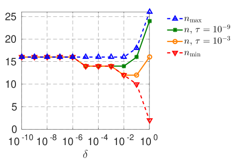
Figure 4.1: The estimated number of iterations $n_{\textrm{max}}$, iteration $n_{\textrm{min}}$ where the acceleration has been turned off, and total number of iterations $n$ in the SP2-ACC expansion for various values of $\delta$. The recursive expansion is applied to the matrix $X_{0}=\text{diag}(0.48,0.52)$ perturbed in each iteration by a diagonal matrix with random elements from a normal distribution and with spectral norm $\tau$.

There is no need for accurate detection of the transition between the conditioning and purification phases—the parameter $\delta$ in the algorithm is to some extent arbitrary. A larger $\delta$-value results in less acceleration. A smaller value means that we will start to check the stopping criterion later possibly resulting in superfluous iterations, particularly in low accuracy calculations, see Figure 4.1. By numerical experiments we have found $\delta=0.01$ to be an appropriate value. For values smaller than $0.01$ the effect of the acceleration is less than 1 percent compared to the regular iteration, see Figure 4.2.

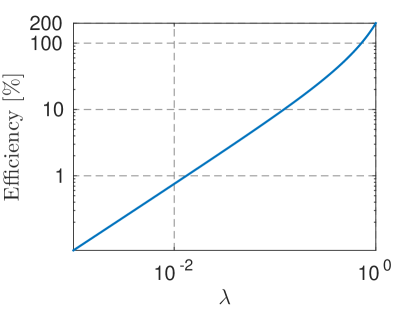
Figure 4.2: Efficiency of the accelerated SP2-ACC scheme relative to the regular SP2 scheme. The figure shows how much more an unoccupied eigenvalue $\lambda$ is reduced by the polynomial $(1-\alpha+\alpha\lambda)^{2}$ with $\alpha=2/(2-\lambda)$ compared to the polynomial $\lambda^{2}$, in the relative sense, i.e. $|\lambda^{2}-(1-\alpha+\alpha\lambda)^{2}|/|\lambda-\lambda^{2}|$. The corresponding (identical) figure for an occupied eigenvalue can be constructed in the same way. Clearly the acceleration has almost no effect in the purification phase when all eigenvalues are close to their desired values of 0 or 1. The plot is in log-log scale.

4.1 Estimation of the order of convergence

As for the McWeeny expansion one may want to use the Frobenius norm instead of the spectral norm to measure the idempotency error. However, for the SP2 expansion, relation (2.17) translates to

$$K_{i-2}^{2}/K_{i}\geq 1,\quad\textrm{if }p_{i}\neq p_{i-1}$$ (4.11)

given second order convergence and the application of Theorem 1 for compositions of alternating polynomials from two iterations. We have not been able to prove that (4.11) always holds. However, we have also not been able to find any counterexample where (4.11) does not hold in exact arithmetics.

We have encountered cases when (4.11) does not hold due to numerical errors. However, the use of the Frobenius norm has not resulted in too early stops in those cases. An example is given in Figure 4.3 where we applied the recursive expansion to a random symmetric dense matrix. The occupied and unoccupied eigenvalues were distributed equidistantly in $[0,\ 0.495]$ and $[0.505,\ 1]$, respectively. The eigenvectors of the matrix were taken from a QR factorization of a matrix with random elements from a normal distribution. The use of the Frobenius norm in the stopping criterion results in a stop in iteration 29 while the use of the spectral norm results in a stop in iteration 31. However, being clear from panels (c) and (d), the stagnation phase started already in iteration 29. Although (4.11) does not hold, the use of the Frobenius norm does not result in a too early stop in this case.

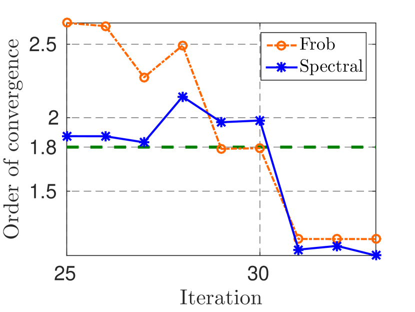
a Observed and estimated orders of convergence

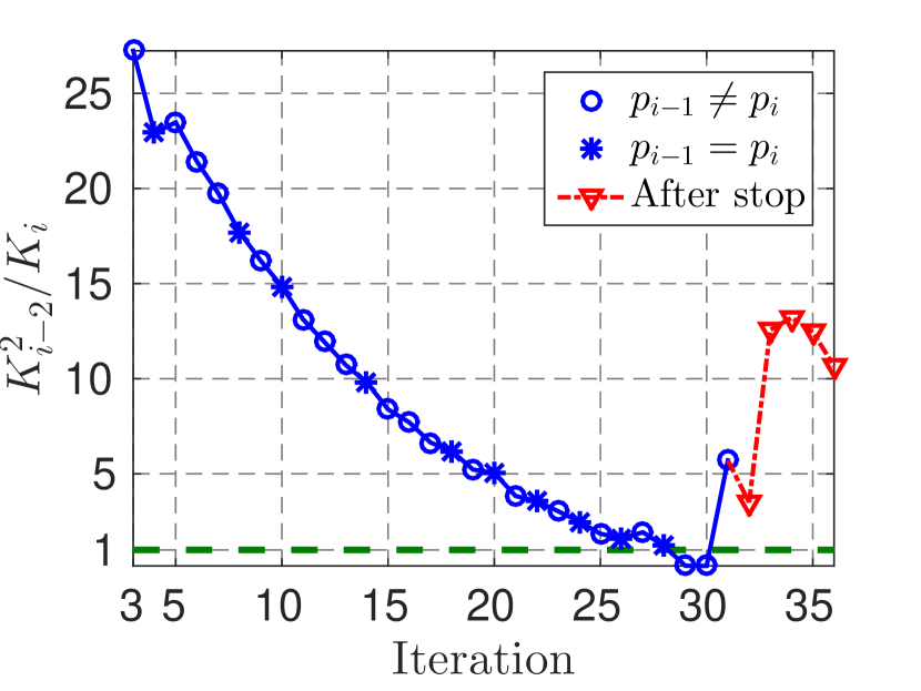
b ${K_{i-2}^{2}}/{K_{i}}$
 

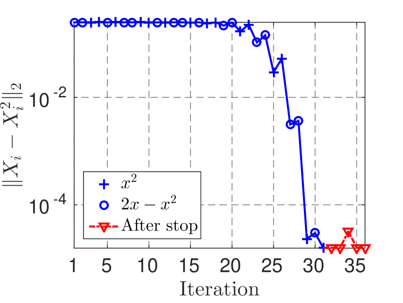
c Idempotency error using
spectral norm

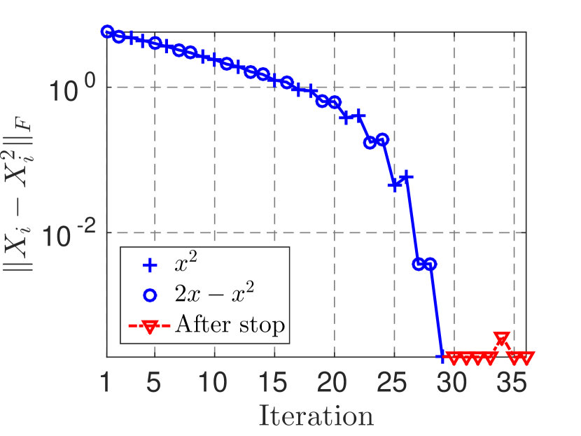
d Idempotency error using
Frobenius norm

Figure 4.3: Example illustrating a special case when use of the Frobenius norm in the stopping criterion results in an earlier stop than use of the spectral norm. The regular SP2 expansion is applied to a random symmetric dense $1000\times 1000$ matrix with all eigenvalues in $[0,\ 1]$, homo-lumo gap 0.01 located symmetrically around 0.5, and occupation number 500. In each iteration $i$ the matrix $X_{i}$ is perturbed by a random symmetric matrix with elements from a normal distribution and with spectral norm $10^{-5}$.

4.2 Number of subsequent iterations with the same polynomial

The stopping criteria in Algorithms 3 and 5 include a condition of alternating polynomials, i.e. that $p_{i}\neq p_{i-1}$ in iteration $i$. When the polynomials in each iteration are chosen based on the trace of the matrix as in Algorithm 3, it is possible to construct examples where the same polynomial appears in an arbitrary number of subsequent iterations. In particular, you will get a large number of consecutive iterations with the same polynomial if there are many eigenvalues clustered very close to either the homo or the lumo eigenvalue. However, besides artificially constructed matrices we have not come across Fock or Kohn–Sham matrices that give more than a few subsequent iterations with the same polynomial. When the polynomials are chosen based on the location of the homo and lumo eigenvalues as in Algorithm 4, the number of subsequent iterations is strictly bounded. When Algorithm 4 is used without acceleration there can after an initial startup phase be at most two subsequent iterations with the same polynomial, as shown by the following theorem.

Theorem 2.

In Algorithm 4, let $\beta_{\textrm{up}}\neq 0$, $\gamma_{\textrm{up}}\neq 0$, $\beta_{\textrm{lo}}=0$, and $\gamma_{\textrm{lo}}=0$. Assume that $p_{i}\neq p_{i-1}$. Then, if $p_{i+1}=p_{i}$ it follows that $p_{i+2}\neq p_{i+1}$.

Proof.

We use here the notation

$$\beta_{i}\coloneqq\beta_{\textrm{up}}\quad\textrm{and}\quad\gamma_{i}\coloneqq\gamma_{\textrm{up}}$$ (4.12)

in every iteration $i$ of the recursive expansion. Without loss of generality we consider the case $i=2$. Assume that $p_{1}=1$. Then, $\beta_{0}\leq\gamma_{0}$ and the largest possible number of subsequent iterations with $p_{k}=0,\ k\geq 2$ is obtained with $\beta_{0}=\gamma_{0}$. Then, following Algorithm 4 we have that

$$\gamma_{1} =\gamma_{0}^{2},$$ (4.13)

$$\beta_{1} =2\beta_{0}-\beta_{0}^{2}=2\gamma_{0}-\gamma_{0}^{2}.$$ (4.14)

Since $\beta_{1}>\gamma_{1}$, $p_{2}=0$ and

$$\gamma_{2} =2\gamma_{1}-\gamma_{1}^{2}=2\gamma_{0}^{2}-\gamma_{0}^{4},$$ (4.15)

$$\beta_{2} =\beta_{1}^{2}=(2\gamma_{0}-\gamma_{0}^{2})^{2}=2\gamma_{0}^{2}-\gamma_{0}^{4}+2\gamma_{0}^{2}(\gamma_{0}-1)^{2}.$$ (4.16)

Then, since $2\gamma_{0}^{2}(\gamma_{0}-1)^{2}>0$, we have that $\beta_{2}>\gamma_{2}$ and $p_{3}=0$. Therefore

$$\gamma_{3} =2\gamma_{2}-\gamma_{2}^{2}=2(2\gamma_{0}^{2}-\gamma_{0}^{4})-(2\gamma_{0}^{2}-\gamma_{0}^{4})^{2}=4\gamma_{0}^{2}-6\gamma_{0}^{4}+4\gamma_{0}^{6}-\gamma_{0}^{8},$$ (4.17)

$$\beta_{3} =\beta_{2}^{2}=(2\gamma_{0}-\gamma_{0}^{2})^{4}$$

$$=\underbrace{4\gamma_{0}^{2}-6\gamma_{0}^{4}+4\gamma_{0}^{6}-\gamma_{0}^{8}}_{\gamma_{3}}\underbrace{-4\gamma_{0}^{2}(2-11\gamma_{0}^{2}+16\gamma_{0}^{3}-10\gamma_{0}^{4}+4\gamma_{0}^{5}-\gamma_{0}^{6})}_{<0}.$$ (4.18)

Thus, $\beta_{3}<\gamma_{3}$ and $p_{4}=1$. The case with $p_{1}=0$ can be shown similarly. ∎∎

Note that Theorem 2 does not exclude the possibility of a large number of initial iterations with the same polynomial. However, as soon as each of the two polynomials has been used at least once, there will not be more than two subsequent iterations with the same polynomial. For Algorithm 4 with acceleration, it is possible to show that there cannot be more than three subsequent iterations with the same polynomial.

5 Numerical experiments

This section provides numerical illustrations of the proposed stopping criteria showing that they work well for dense and sparse matrices regardless of what method is used to select matrix elements for removal. All tests in this section are performed in Matlab R2015b. We will here use the regular SP2 expansion without acceleration. Similar results can be shown for expansions with other polynomials, such as McWeeny or accelerated SP2. It will be assumed that non-overlapping intervals containing the homo and lumo eigenvalues, respectively, are known before the start of the expansion so that Algorithm 4 can be used for selection of polynomials and Algorithm 5 for the expansion. To get a regular (nonaccelerated) expansion the parameters $\beta_{\textrm{lo}}$ and $\gamma_{\textrm{lo}}$ are both set to 0 on lines 3 and 5 of Algorithm 4 giving scaling parameters $\alpha_{i},i=1,2,\dots$ on lines 17 and 22 equal to 1 and $n_{\textrm{min}}$ equal to 2.

In our first test we apply the SP2 expansion to a random symmetric dense matrix, see Figure 5.1. The eigenvectors of the matrix were taken from a QR factorization of a matrix with random elements from a normal distribution. The occupied and unoccupied eigenvalues were distributed equidistantly in $[0,\ 0.49]$ and $[0.51,\ 1]$, respectively. In each iteration, the matrix $X_{i}$ was perturbed by a random symmetric matrix with spectral norm $\tau$ and elements from a normal distribution. The spectral norm was used to compute the observed order of convergence used in the stopping criterion. The figure shows that the stopping criterion accurately detects when numerical errors start to dominate the calculation and prevent any further improvement of the eigenvalues.

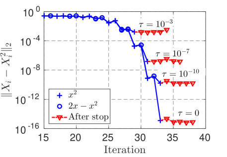
Figure 5.1: Idempotency error in each iteration of the SP2 expansion for a random symmetric dense $200\times 200$ matrix with spectrum in $[0,\ 1]$ and homo-lumo gap 0.02 located around 0.5 and occupation number 100. In each iteration the matrix was perturbed by a random symmetric matrix with spectral norm $\tau$. The idempotency error is shown for 4 different values of $\tau$, before (blue circles and plus signs) and after (red triangles) the stop.

We show in Figure 5.2 that the stopping criteria work well for two different approaches to select matrix elements for removal in a linear scaling sparse matrix setting. The Fock matrix comes from a converged spin-restricted Hartree–Fock calculation for a linear alkane molecule C₁₆₀H₃₂₂ using the standard Gaussian basis set STO-3G, giving a total of 1122 basis functions and 641 occupied orbitals. In this case the eigenvalue problem (1.1) is on generalized form

$$Fx_{i}=\lambda_{i}Sx_{i},$$ (5.1)

where $S$ is the basis set overlap matrix. A congruence transformation employing the inverse Cholesky factor of $S$ is used to get the eigenvalue problem on standard form as required by the algorithms described in this article. There are three different common approaches for removal of matrix elements. Each matrix element in a Fock or density matrix usually corresponds to the distance between two atomic nuclei. In cutoff radius based truncation, all elements corresponding to distances larger than a predefined cutoff radius are removed. However, in methods employing the congruence transformation this approach cannot be straightforwardly applied. In element magnitude based truncation, all elements with absolute value smaller than a predefined threshold value are removed. The threshold value is typically chosen based on practical experience without being directly linked to the actual error in the final result, the density matrix. However, a surprisingly simple relationship between the truncation and the error in the final result was developed by Rubensson et al. ⁸, allowing us to control the forward error $\|D-\widetilde{X}_{n}\|_{2}$. The forward error is split in two parts, the error in eigenvalues (idempotency error) and the error in the occupied subspace. The subspace error is due to numerical errors and the eigenvalue error is due to numerical errors and a finite number of iterations. Figure 2a shows that our stopping criteria work well together with truncation based on matrix element magnitude. Figure 2b shows that our stopping criteria work well when matrix elements are removed with control of the subspace error ⁸.

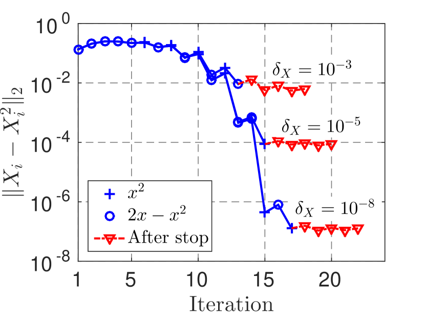
a Truncation based on the
magnitude relation

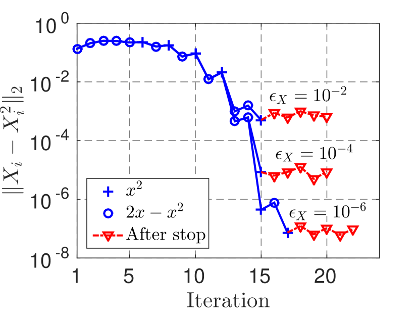
b Truncation based on the
spectral norm of the error matrix

Figure 5.2: Demonstration of the stopping criterion with different ways of selecting matrix elements for removal in a sparse matrix setting. The idempotency error in each iteration of the SP2 expansion is shown for a Fock matrix coming from a Hartree–Fock calculation on a linear alkane using a standard Gaussian basis set. Panel (a): Magnitude based truncation with threshold value $\delta_{X}$ for removing small matrix elements. Panel (b): Removal of elements with control of the error in the occupied subspace with the requirement that $\sin\theta<\epsilon_{X}$ where $\theta$ is the largest canonical angle between the exact and perturbed subspaces.

We will now investigate how the stopping criterion works when the observed order is estimated using the Frobenius and mixed matrix norms. We apply the SP2 expansion to a diagonal matrix of dimension $10^{8}\times 10^{8}$ with occupation number $10^{8}/2$, homo-lumo gap 0.1 located symmetrically around 0.5 and with otherwise equidistant eigenvalues in $[0,\ 1]$. The idempotency errors in each iteration measured by the Frobenius, mixed, and spectral norms are shown in Figure 5.3. The block size for the mixed norm is 1000. As anticipated in Section 2, $\|X_{i}-X_{i}^{2}\|_{F}$ never goes below 1 for such a large system and (2.19) cannot be used to estimate the observed order. If the spectral norm is expensive to compute, the mixed norm may be used in such cases.

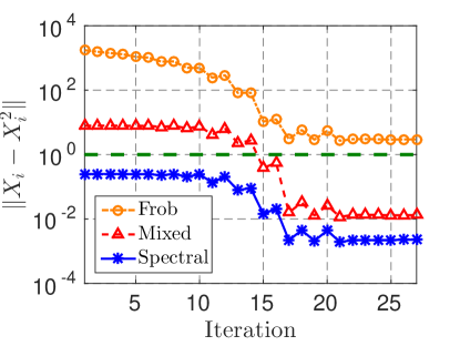
Figure 5.3: Frobenius, mixed, and spectral norms of $X_{i}-X_{i}^{2}$ in every iteration $i$ of the recursive SP2 expansion applied to a diagonal $10^{8}\times 10^{8}$ matrix with occupation number $10^{8}/2$, homo-lumo gap 0.1 located symmetrically around 0.5, and otherwise equidistantly distributed eigenvalues in $[0,\ 1]$. In each iteration the matrix was perturbed by a diagonal matrix with random elements from a normal distribution and with spectral norm $10^{-3}$. The block size for the mixed norm is 1000.

6 Application to self-consistent field calculations

In this section we use the developed stopping criteria in the regular and accelerated SP2 expansions in self-consistent field (SCF) calculations with the quantum chemistry program Ergo ^{16, 17}. We have performed spin-restricted Hartree–Fock calculations on a cluster of 4158 water molecules using the standard Gaussian basis set 3-21G, giving a total of 54054 basis functions. As initial guess we used the result of a calculation with a smaller basis set, STO-3G. We used direct inversion in the iterative subspace (DIIS) for convergence acceleration ^{34, 35} and stopped the iterations as soon as the largest absolute element of $FDS-SDF$ was smaller than $10^{-3}$. The hierarchical matrix library  ³⁶ was used for sparse matrix operations. A block size of 32 was used at the lowest level in the sparse hierarchical representation. The mixed norm with block size 32 was used both in the stopping criterion and for removal of small matrix elements ³¹ with a tolerance of $10^{-3}$ for the error in the occupied subspace measured by the largest canonical angle between the exact and approximate subspaces ⁸.

The tests were running on the Tintin cluster at the UPPMAX computer center in Uppsala University using the gcc 5.3.0 compiler and the OpenBLAS ³⁷ library was used for matrix operations at the lowest level in the sparse hierarchical representation. Each node on Tintin is a dual AMD Bulldozer compute server with two 8-core Opteron 6220 processors running at 3.0 GHz. The calculations presented here are performed on a node with 128 GB of memory.

In each SCF cycle we compute upper and lower bounds of the homo and lumo eigenvalues and propagate them to the next SCF cycle. It was shown by Rubensson and Zahedi ³⁸ that eigenvalues around the homo-lumo gap can be computed efficiently by making use of the ability of the recursive expansion to give large separation between interior eigenvalues. In that work, the Lanczos method was used to extract the desired information. Here we use a recent approach to compute accurate homo and lumo bounds that only requires the evaluation of Frobenius norms and traces during the course of the recursive expansion ³⁰. Intervals containing the homo and lumo eigenvalues are propagated between SCF cycles using Weyl’s theorem for eigenvalue movement ^{30, 8}. The inner bounds for the homo and lumo eigenvalues are used both for the determination of polynomials in Algorithm 4 and for the error control. The outer bounds are used for the acceleration in Algorithm 4. When inner bounds for homo and lumo are not known or are not accurate we fall back to the trace-correcting SP2 expansion described in Algorithm 3. However, even if the outer bounds are loose Algorithm 4 can be used with a modification that the polynomials are determined on the fly using the condition in Line 7 in Algorithm 3.

The regular and accelerated SP2 expansions are compared in Figure 6.1.

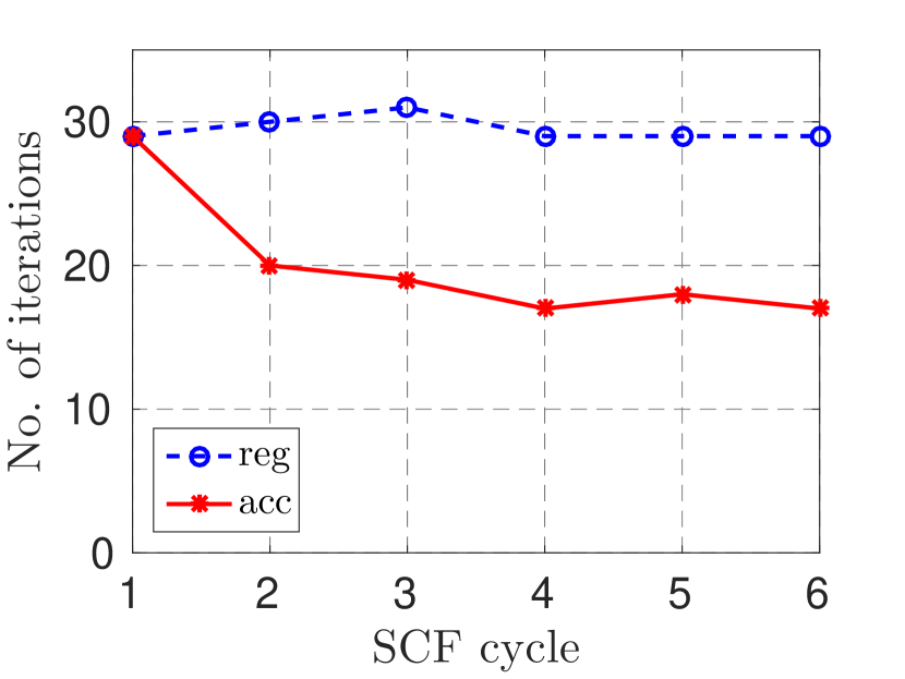
a Number of iterations in the recursive expansion

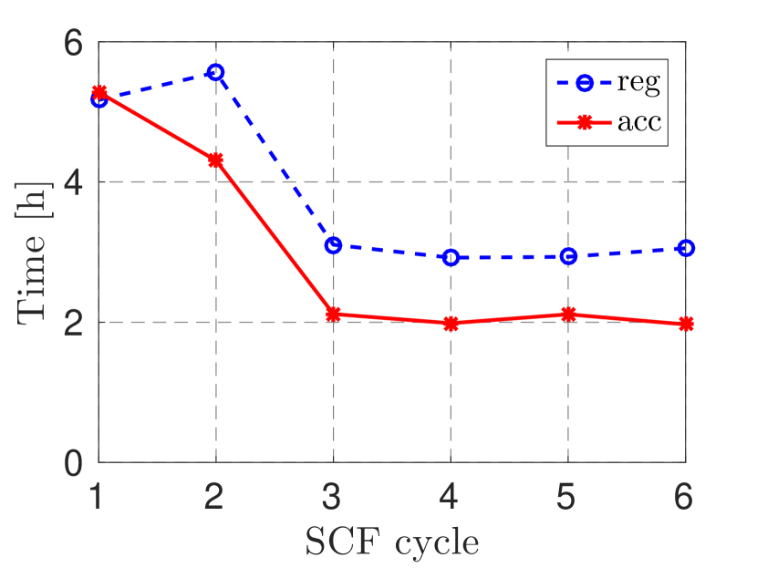
b Recursive expansion wall time

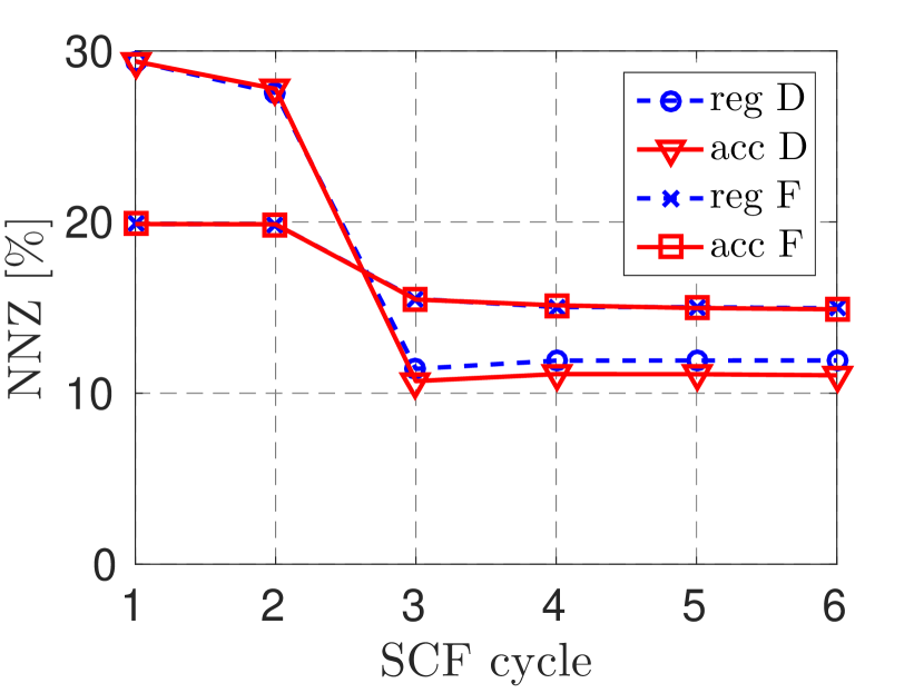
c Number of non-zeros

Figure 6.1: Comparison of the regular and accelerated SP2 expansions in a self-consistent field Hartree–Fock calculation for a water cluster with 4158 water molecules. Panels (a) and (b) show the number of iterations and wall time of the recursive expansion in each self-consistent field cycle. Panel (c) gives the percentage of non-zero elements in the Fock and density matrices, $F$ and $D$ respectively, in orthogonal basis. See the text for more details.

Panels (a) and (b) show the number of iterations and wall time, respectively, for the regular and accelerated expansions in each SCF cycle. Panel (c) shows the percentage of non-zero elements in the Fock and density matrices in orthogonal basis in each SCF cycle. Matrices were transformed from non-orthogonal basis using the inverse Cholesky factor as in the previous section. The number of non-zeros and the idempotency error for the regular and accelerated SP2 expansions in the last SCF cycle are shown in Figure 6.2. In this case, the accelerated expansion takes a shorter but less sparse route to the final density matrix. Thus, the peak memory usage is larger and in some iterations significantly more work is required. However, the acceleration gives a substantial reduction of the overall computational time needed for the recursive expansion.

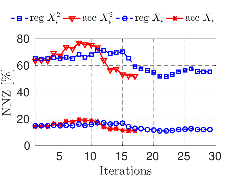
a Number of non-zeros

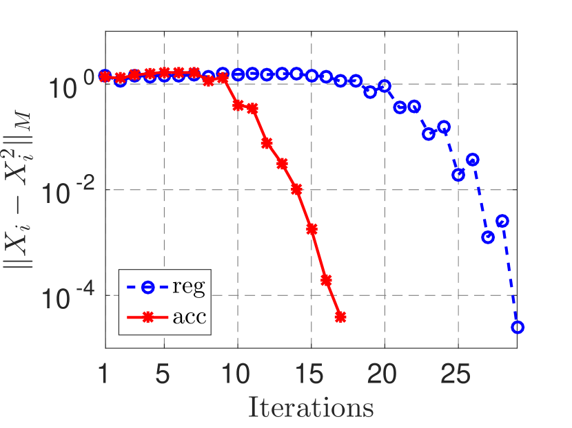
b Idempotency error measured using the mixed norm

Figure 6.2: Comparison of the regular and accelerated SP2 expansions in the last cycle in a self-consistent field Hartree–Fock calculation for a water cluster with 4158 water molecules.

Figure 6.3 shows for each SCF cycle intervals containing the homo and lumo eigenvalues propagated from the previous SCF cycle (initial homo/lumo) and the improved intervals computed using information extracted from the recursive expansion (estimated homo/lumo).

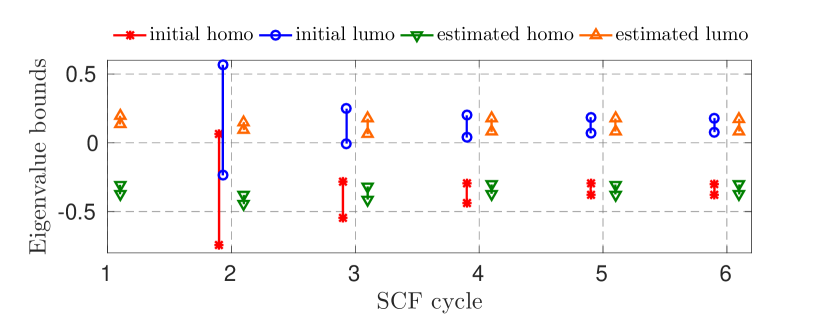
Figure 6.3: For each cycle in a self-consistent field Hartree–Fock calculation for a water cluster with 4158 water molecules with the SP2-ACC expansion, intervals containing the homo and lumo eigenvalues propagated from the previous SCF cycle (initial) and computed as a by-product of the recursive expansion (estimated). The corresponding figure for regular SP2 is essentially identical.

Table 1 shows upper and lower bounds $n_{\textrm{max}}$ and $n_{\textrm{min}}$, respectively, and actual number of iterations $n$ in the recursive expansion in each SCF cycle. In the two initial SCF cycles the homo and lumo intervals are overlapping, see Figure 6.3, and therefore we cannot use Algorithm 4 to determine the sequence of polynomials. Thus, an upper bound of the number of iterations $n_{\textrm{max}}$ based on the homo and lumo intervals cannot be computed. The acceleration has an effect as soon as the outer bounds for homo and lumo are better than the extremal bounds ($\lambda_{\textrm{min}}$ and $\lambda_{\textrm{max}}$), in our case already in the second SCF cycle. However, in the initial SCF cycles the outer bounds are loose, making the acceleration less effective than in later iterations. Starting from the third SCF cycle the upper and lower bounds on the number of iterations are given by Algorithm 4. In iteration $n_{\textrm{min}}$ the acceleration has been turned off, as discussed in Section 4. Note that the proposed stopping criteria are used in each SCF cycle independently of the method for choosing polynomials. The recursive expansion is stopped as soon as the estimated order of convergence computed using the mixed norm is smaller than $\tilde{q}=1.8$.

Table 1: Upper estimate $n_{\textrm{max}}$, actual number of iterations $n$ in recursive expansion in each SCF cycle and the iteration $n_{\textrm{min}}$ where the acceleration has been turned off. There is no acceleration in the first SCF cycle, and at least two iterations should be performed to be able to check the stopping criterion.

SCF cycle	1	2	3	4	5	6
$n_{\textrm{max}}$	-	-	26	24	24	23
$n$	29	20	19	17	18	17
$n_{\textrm{min}}$	2	14	14	14	14	14

The proposed stopping criteria, the acceleration technique and efficient estimation of the homo and lumo eigenvalues give a significant performance improvement of the recursive density matrix expansion. We show with the water cluster example that the use of the SP2-ACC polynomials reduces the number of matrix-matrix multiplications in comparison to the regular SP2 scheme and the proposed stopping criteria enable us to reach the level of attainable accuracy without spending redundant computational effort in the stagnation phase.

The length of the conditioning phase depends on the homo-lumo gap. Smaller homo-lumo gap will give a longer phase. The acceleration technique reduces the length of the conditioning phase, but has no significant impact in the purification phase. Our stopping criteria are designed to automatically detect when numerical errors start to dominate. By introducing a parameter $C_{q}$ satisfying (2.4) we eliminate the need to determine an iteration after which one can check the stopping criterion. The proposed stopping criteria can be checked already in the first iteration. Their efficiency depends on the closeness of the chosen value $C_{q}$ to the smallest value satisfying (2.4), but does not depend on the length of phases in the recursive expansion, and is thus independent of the homo-lumo gap.

7 Discussion

The stopping criterion is an important aspect of the development process of any iterative method. Many works address this question for linear systems ^{39, 40, 41, 42, 43} and eigensolvers ^{44, 45, 46}. In general, such stopping criteria are based on controlling the norm of a suitable residual or estimate of the norm of the error. The convergence path can be irregular and contain stagnation regions.

Stopping criteria for iterative methods for matrix functions are often based on the relative distance of the subsequent iterates $X_{k}$ and $X_{k+1}$ ⁶. As soon as the distance becomes smaller than some predefined threshold value the iterations stop. However, in the presence of numerical errors it is hard to find an optimal threshold value. To illustrate that our approach to develop stopping criteria for iterative methods is applicable also to other matrix iterations, we derive a stopping criterion of the same type for the Newton sign matrix iteration in Appendix A.

Newton’s method to find roots of real-valued functions is locally at least quadratically convergent for simple roots. Also in this case, the iterations are typically stopped when some error measure goes below a predefined threshold value. Often one wants to continue iterating until numerical errors (from e.g. floating point roundoff) prevent any further decrease of the error. The threshold value is often chosen in terms of the expected accuracy of the evaluation of the function, e.g. some multiple of machine epsilon. To avoid the selection of threshold value one may, following the lines of the present work, analyze the convergence behavior and devise a stopping criterion based on the detection of a fall in convergence order, see Appendix B. This is in particular useful in cases when the accuracy in the evaluation of a function is not known or depends non-trivially on program input parameters.

8 Concluding remarks

Recursive expansions to compute the density matrix in electronic structure calculations are usually stopped when the idempotency error goes below some predefined tolerance. The main problem with such an approach is that an appropriate value for the tolerance is difficult to select. If the tolerance is small in relation to numerical errors coming from removal of matrix elements or rounding errors, the iterations will never stop. If the tolerance is large in relation to numerical errors, the same accuracy could be achieved with less effort.

In previous work we addressed the never stop issue by tightening the tolerance for removal of small matrix elements at the end of the expansion until the desired accuracy is achieved for eigenvalues ⁸. However, this approach also involves a user defined parameter for the accuracy in eigenvalues with potential impact on convergence and computational cost.

The practical usefulness of our new stopping criteria proposed here can be seen in the context of the Ergo ^{16, 17} program where the new stopping criterion allows the number of input parameters to the program to be reduced, since only a single parameter for the density matrix construction accuracy is now needed. The new stopping criterion also solves previous problems with failed convergence when using default Ergo parameters; previously, when using the default parameters the recursive expansion failed due to rounding errors in some cases, particularly for larger molecules where the effect of rounding errors is more pronounced.

If the homo and lumo eigenvalues are known in advance one may compute an upper bound for the number of iterations in advance by iterating until the homo and lumo eigenvalues are within rounding error from their desired values. The number of iterations in such an approach corresponds to $n_{\textrm{max}}$ in the present work. For high accuracy calculations this may be a reasonable approach but often it would lead to superfluous iterations, as for example can be seen for the water cluster calculations in Section 6.

In the present work three phases of the recursive expansion were identified: conditioning, purification, and stagnation. The appropriate moment to stop the expansion is at the transition between purification and stagnation. At this transition there is a drop in the order of convergence. By detection of this drop we are able to stop the expansion at the appropriate moment without any user defined parameters. The transition to stagnation is accurately detected even if the idempotency error continues to slowly decrease. By altering the asymptotic error constant in the observed order of convergence we avoid an early stop in the conditioning phase.

Support from the Göran Gustafsson foundation, the Swedish research council (grant no. 621-2012-3861), the Lisa and Carl–Gustav Esseen foundation, and the Swedish national strategic e-science research program (eSSENCE) is gratefully acknowledged. Computational resources were provided by the Swedish National Infrastructure for Computing (SNIC) at Uppsala Multidisciplinary Center for Advanced Computational Science (UPPMAX).

Appendix A Sign matrix iterations

Applying Newton’s method to the function $f(X)=X^{2}-I$ gives an iteration

$$X_{k+1}=\frac{1}{2}(X_{k}^{-1}+X_{k}),\quad X_{0}=A,$$ (A.1)

for the sign matrix function which converges quadratically provided that $A\in\mathbb{C}^{n\times n}$ has no eigenvalues on the imaginary axis ⁶.

Since the matrices $X_{k}$ and $X_{k+1}-X_{k}$ commute, the Taylor expansion of the matrix function $f(X_{k+1})=X_{k+1}^{2}-I$ is given by ^{47, 48}

$$f(X_{k+1}) =f(X_{k})+f^{\prime}(X_{k})(X_{k+1}-X_{k})+R_{2}(X_{k})$$ (A.2)

$$=f(X_{k})+f^{\prime}(X_{k})(-(f^{\prime}(X_{k}))^{-1}f(X_{k}))+R_{2}(X_{k})$$ (A.3)

$$=R_{2}(X_{k}),$$ (A.4)

where the truncation error for the spectral norm ⁴⁹ is bounded

$$\|R_{2}(X_{k})\|_{2} \leq\frac{1}{2}\|X_{k+1}-X_{k}\|_{2}^{2}\max_{s\in[0,1]}\|f^{\prime\prime}(X_{k}+s(X_{k+1}-X_{k}))\|_{2}$$ (A.5)

$$\leq\frac{1}{2}\|f(X_{k})\|_{2}^{2}\|(f^{\prime}(X_{k}))^{-1}\|_{2}^{2}\max_{s\in[0,1]}\|f^{\prime\prime}(X_{k}+s(X_{k+1}-X_{k}))\|_{2}$$ (A.6)

$$=\frac{1}{4}\|X_{k}^{-1}\|_{2}^{2}\|f(X_{k})\|_{2}^{2},$$ (A.7)

where we have used that $f^{\prime}(X_{k})=2X_{k}$ and $f^{\prime\prime}(X_{k})=2I$.

Thus in exact arithmetics

$$\|f(X_{k+1})\|_{2}\leq\frac{1}{4}\|X_{k}^{-1}\|_{2}^{2}\|f(X_{k})\|_{2}^{2},$$ (A.8)

which suggests to stop the iterations as soon as

$$\|f(X_{k})\|_{2}<1\quad\text{and}\quad\frac{\log(\|f(X_{k+1})\|_{2}/C_{k})}{\log(\|f(X_{k})\|_{2})}\leq 1.8,$$ (A.9)

where

$$C_{k}\geq\frac{1}{4}\|X_{k}^{-1}\|_{2}^{2}.$$ (A.10)

The value of $C_{k}$ should be chosen the smallest possible, see the discussion in section 2.

If in addition we assume that the matrix $A$ is normal, then for $k\geq 1$ the absolute values of the eigenvalues of $X_{k}$ are bounded from below by 1 and $\|X_{k}^{-1}\|_{2}^{2}\leq 1$. Thus for all $k\geq 1$ we define

$$C_{k}:=C=\frac{1}{4}.$$ (A.11)

Appendix B Stopping criteria for Newton’s method

Let $f(x)$ be a twice continuously differentiable function, $f(x^{*})=0$, and $f^{\prime}(x^{*})\neq 0$. Then, Newton’s method

$$x_{k+1}=x_{k}+\Delta x_{k},\quad\Delta x_{k}=-\frac{f(x_{k})}{f^{\prime}(x_{k})}$$ (B.1)

is locally quadratically convergent to $x^{*}$.

Assume that $f^{\prime}(x_{k})\neq 0$. Taylor expansion around $x_{k}$ with step $\Delta x_{k}$ and using (B.1) and Lagrange’s form of the remainder gives

$$f(x_{k+1}) =\frac{f^{\prime\prime}(\xi_{k})}{2(f^{\prime}(x_{k}))^{2}}(f(x_{k}))^{2}$$ (B.2)

where $\xi_{k}$ is some value between $x_{k}$ and $x_{k+1}$. Following the ideas of the present article, this suggests the stopping criterion: stop as soon as

$$|f(x_{k})| <1\quad\textrm{ and }\quad\frac{\log|f(x_{k+1})/C_{k}|}{\log|f(x_{k})|}<1.8,$$ (B.3)

where

$$C_{k}=\frac{F_{k}}{2(f^{\prime}(x_{k}))^{2}},\quad F_{k}\geq\max_{\xi\textrm{ between }x_{k}\textrm{ and }x_{k+1}}|f^{\prime\prime}(\xi)|.$$ (B.4)

We note that if $f^{\prime}(x_{k})$ comes close to zero $C_{k}$ becomes very large and the stopping criterion is not triggered. Thus, there is no need for special treatment in such cases.

References

- Roothaan 1951 Roothaan, C. C. J. Rev. Mod. Phys. 1951, 23, 69–89
- Hohenberg and Kohn 1964 Hohenberg, P.; Kohn, W. Phys. Rev. 1964, 136, B864–B871
- Kohn and Sham 1965 Kohn, W.; Sham, L. J. Phys. Rev. 1965, 140, 1133
- Bowler and Miyazaki 2012 Bowler, D. R.; Miyazaki, T. Rep. Prog. Phys. 2012, 75, 036503
- Goedecker and Colombo 1994 Goedecker, S.; Colombo, L. Phys. Rev. Lett. 1994, 73, 122–125
- Higham 2008 Higham, N. J. Functions of matrices: theory and computation; SIAM: Philadelphia, 2008
- Rubensson 2012 Rubensson, E. H. SIAM J. Sci. Comput. 2012, 34, B1–B23
- Rubensson et al. 2008 Rubensson, E. H.; Rudberg, E.; Sałek, P. J. Chem. Phys. 2008, 128, 074106
- Rudberg and Rubensson 2011 Rudberg, E.; Rubensson, E. H. J. Phys.: Condens. Matter 2011, 23, 075502
- Benzi et al. 2013 Benzi, M.; Boito, P.; Razouk, N. SIAM Rev. 2013, 55, 3–64
- McWeeny 1956 McWeeny, R. Proc. R. Soc. London Ser. A 1956, 235, 496–509
- Palser and Manolopoulos 1998 Palser, A. H. R.; Manolopoulos, D. E. Phys. Rev. B 1998, 58, 12704–12711
- Niklasson 2002 Niklasson, A. M. N. Phys. Rev. B 2002, 66, 155115
- Rubensson 2011 Rubensson, E. H. J. Chem. Theory Comput. 2011, 7, 1233–1236
- VandeVondele et al. 2012 VandeVondele, J.; Borštnik, U.; Hutter, J. J. Chem. Theory Comput. 2012, 8, 3565–3573
- 16 Rudberg, E.; Rubensson, E. H.; Sałek, P. Ergo (Version 3.4). Available at http://www.ergoscf.org (Accessed 14 June 2016)
- Rudberg et al. 2011 Rudberg, E.; Rubensson, E. H.; Sałek, P. J. Chem. Theory Comput. 2011, 7, 340–350
- Bock et al. 2014 Bock, N.; Challacombe, M.; Gan, C. K.; Henkelman, G.; Nemeth, K.; Niklasson, A. M. N.; Odell, A.; Schwegler, E.; Tymczak, C. J.; Weber, V. FreeON. 2014; Los Alamos National Laboratory (LA-CC 01-2; LA-CC-04-086), Copyright University of California.
- Qin et al. 2015 Qin, X.; Shang, H.; Xiang, H.; Li, Z.; Yang, J. Int. J. Quantum Chem. 2015, 115, 647–655
- Cawkwell and Niklasson 2012 Cawkwell, M. J.; Niklasson, A. M. N. J. Chem. Phys. 2012, 137, 134105
- Borštnik et al. 2014 Borštnik, U.; VandeVondele, J.; Weber, V.; Hutter, J. Parallel Comput. 2014, 40, 47–58
- Cawkwell et al. 2014 Cawkwell, M. J.; Wood, M. A.; Niklasson, A. M. N.; Mniszewski, S. M. J. Chem. Theory Comput. 2014, 10, 5391–5396
- Chow et al. 2015 Chow, E.; Liu, X.; Smelyanskiy, M.; Hammond, J. R. J. Chem. Phys. 2015, 142, 104103
- Weber et al. 2015 Weber, V.; Laino, T.; Pozdneev, A.; Fedulova, I.; Curioni, A. J. Chem. Theory Comput. 2015, 11, 3145–3152
- Daniels and Scuseria 1999 Daniels, A. D.; Scuseria, G. E. J. Chem. Phys. 1999, 110, 1321–1328
- Mazziotti 2003 Mazziotti, D. A. Phys. Rev. E 2003, 68, 066701
- Shao et al. 2003 Shao, Y.; Saravanan, C.; Head-Gordon, M.; White, C. A. J. Chem. Phys. 2003, 118, 6144–6151
- Suryanarayana 2013 Suryanarayana, P. Chem. Phys. Lett. 2013, 555, 291–295
- 29 Note that only two phases were identified in the previous work of Rubensson and Niklasson 30. Here, a third stagnation phase is identified.
- Rubensson and Niklasson 2014 Rubensson, E. H.; Niklasson, A. M. N. SIAM J. Sci. Comput. 2014, 36, B147–B170
- Rubensson and Rudberg 2011 Rubensson, E. H.; Rudberg, E. J. Comput. Chem. 2011, 32, 1411–1423
- Holas 2001 Holas, A. Chem. Phys. Lett. 2001, 340, 552–558
- Mazziotti 2001 Mazziotti, D. A. J. Chem. Phys. 2001, 115, 8305–8311
- Pulay 1980 Pulay, P. Chem. Phys. Lett. 1980, 73, 393
- Pulay 1982 Pulay, P. J. Comput. Chem. 1982, 3, 556
- Rubensson et al. 2007 Rubensson, E. H.; Rudberg, E.; Sałek, P. J. Comput. Chem. 2007, 28, 2531–2537
- 37 OpenBLAS (Version 0.2.16). Available at http://www.openblas.net (Accessed 14 June 2016)
- Rubensson and Zahedi 2008 Rubensson, E. H.; Zahedi, S. J. Chem. Phys. 2008, 128, 176101
- Arioli et al. 1992 Arioli, M.; Duff, I.; Ruiz, D. SIAM J. Matrix Anal. Appl. 1992, 13, 138–144
- Arioli et al. 2013 Arioli, M.; Georgoulis, E. H.; Loghin, D. SIAM J. Sci. Comput. 2013, 35, A1537–A1559
- Axelsson and Kaporin 2001 Axelsson, O.; Kaporin, I. Numer. Linear Algebra Appl. 2001, 8, 265–286
- Frommer and Simoncini 2008 Frommer, A.; Simoncini, V. SIAM J. Sci. Comput. 2008, 30, 1387–1412
- Kaasschieter 1988 Kaasschieter, E. BIT Numer. Math. 1988, 28, 308–322
- Bennani and Braconnier 1994 Bennani, M.; Braconnier, T. CERFACS, Toulouse, France, Tech. Rep. TR/PA/94/22 1994,
- Golub and Ye 2000 Golub, G. H.; Ye, Q. BIT Numer. Math. 2000, 40, 671–684
- Vömel et al. 2008 Vömel, C.; Tomov, S. Z.; Marques, O. A.; Canning, A.; Wang, L.-W.; Dongarra, J. J. J. Comput. Phys. 2008, 227, 7113–7124
- Al-Mohy and Higham 2009 Al-Mohy, A. H.; Higham, N. J. Numer. Algorithms 2009, 53, 133–148
- Deadman and Relton 2016 Deadman, E.; Relton, S. D. Linear Algebra Appl. 2016, 504, 354 – 371
- Mathias 1993 Mathias, R. SIAM J. Matrix Anal. Appl. 1993, 14, 1061–1063