Basin structure of optimization based state and parameter estimation

Abstract

Most data based state and parameter estimation methods require suitable initial values or guesses to achieve convergence to the desired solution, which typically is a global minimum of some cost function. Unfortunately, however, other stable solutions (e.g., local minima) may exist and provide suboptimal or even wrong estimates. Here we demonstrate for a 9-dimensional Lorenz-96 model how to characterize the basin size of the global minimum when applying some particular optimization based estimation algorithm. We compare three different strategies for generating suitable initial guesses and we investigate the dependence of the solution on the given trajectory segment (underlying the measured time series). To address the question of how many state variables have to be measured for optimal performance, different types of multivariate time series are considered consisting of 1, 2, or 3 variables. Based on these time series the local observability of state variables and parameters of the Lorenz-96 model is investigated and confirmed using delay coordinates. This result is in good agreement with the observation that correct state and parameter estimation results are obtained if the optimization algorithm is initialized with initial guesses close to the true solution. In contrast, initialization with other exact solutions of the model equations (different from the true solution used to generate the time series) typically fails, i.e. the optimization procedure ends up in local minima different from the true solution. Initialization using random values in a box around the attractor exhibits success rates depending on the number of observables and the available time series (trajectory segment).

For many physical processes dynamical models are available but often not all their state variables and (fixed) parameters are known or easily accessible. In meteorology, for example, sophisticated large scale models exist, which have to be continuously adapted to the true temporal changes of temperatures, wind speed, humidity, and other relevant physical quantities. In quantitative biology mathematical models of single neural or cardiac cells or networks may contain many state variables and parameters whose values are not easy to measure (without destroying the system). In such cases, data based estimation methods can be used to determine these unknown states and a parameters by adapting a suitable model to reproduce and predict the measured time series. This approach can be successful only if two conditions are fulfilled: (i) the available data have to provide sufficient information, i.e. the unknown state variables and parameters have to be observable and (ii) the estimation algorithm has to be properly initialized with initial guesses sufficiently close to the true solution. Here, we consider both problems for the Lorenz-96 model and compare different initialization methods in terms of their effective basin sizes.

I Introduction

180(18,262) Copyright 2015 American Institute of Physics. This article may be downloaded for personal use only. Any other use requires prior permission of the author and the American Institute of Physics. The following article appeared in
J. Schumann-Bischoff et al., Chaos 25, 053108 (2015) and may be found at http://dx.doi.org/10.1063/1.4920942. Estimation methods for state variables or (fixed) parameters can be implemented employing synchronization PJK96 ; PKK98 ; JP00 ; SRL09 ; REKASBP14 or optimization methods CGA08 ; B10 ; SBP11 ; SBLP13 , for example. In the literature one can find many examples with successful applications of state and parameter estimation methods even for chaotic systems VTK04 ; ACFK09 ; QA10 ; A13 ; YKRAQ15 . In practice, however, attempts to fit a model (for example, a set of nonlinear ordinary differential equations (ODEs)) to given data may fail. There are many possible reasons for such a failure, including inappropriate models, poor quality of the measured time series (too noisy, too short), or external perturbations not covered by the model. But even with relatively clean data and the right model architecture, estimation may turn out to be difficult, because the available data do not contain sufficient information about the underlying process. Therefore, in this article we address how the success of a given estimation algorithm for a given model depends of the following aspects:

• the number of available observables (in a multivariate time series)

• the available time series (corresponding to some particular trajectory segment)

• and the way the estimation algorithm is initialized (using guesses for the unknown quantities).

The focus in the presented analysis is on models given by ODEs,

$$\frac{\mathrm{d}\mathbf{x}(t)}{\mathrm{d}t} =\mathbf{F}(\mathbf{x}(t),\mathbf{p},t)\,,$$ (1)

and a measurement function,

$$\mathbf{y}(t) =\mathbf{h}(\mathbf{x}(t))\in\mathbb{R}^{L}\,,$$ (2)

representing the model output with a state vector $\mathbf{x}(t)=(x_{1}(t),\dots,x_{D}(t))^{\mathrm{tr}}\in\mathbb{R}^{D}$, and model parameters $\mathbf{p}=(p_{1},\dots,p_{N_{P}})^{\mathrm{tr}}\in\mathbb{R}^{N_{P}}$. Here and in the following the superscript “$\mathrm{tr}$” denotes the transpose. We assume that a multivariate $L$-dimensional (experimental) time series $\{\bm{\eta}(n)\}$ is given consisting of $N+1$ samples $\bm{\eta}(n)\hat{=}\bm{\eta}(t_{n})\in\mathbb{R}^{L}$, analogous to the model output, and measured at times ${\cal{T}}=\{t_{n}=n\cdot\Delta t\mid n=0,1,\dots,N\}$. The observation times $t_{n}$ are equally spaced (with a fixed time step $\Delta t$) and start at $t_{0}=0$. Any solution of Eq. (1) at discrete times $t_{n}=n\cdot\Delta t$ with a fixed time step $\Delta t$ is denoted by $\{\mathbf{x}(n)\}$ and consists of $N+1$ samples $\mathbf{x}(n)\hat{=}\mathbf{x}(t_{n})$ at times $t_{n}\in{\cal{T}}$. If, from the context, $\Delta t$ and the range of $n$ are clear, this information will be dropped in the following. The same convention holds if a solution is denoted by another symbol, for example $\mathbf{z}$ instead of $\mathbf{x}$: the solution $\{\mathbf{z}(n)\}$ consists of $N+1$ samples $\mathbf{z}(n)\hat{=}\mathbf{z}(t_{n})$ measured at times $t_{n}\in{\cal{T}}$.

As an example we use synthetic data from a 9-dimensional Lorenz-96 system Lorenz96 (Sec. II) and an optimization based estimation algorithm SBP11 (Sec. IV). We check the observability of the state variables of the Lorenz-96 model which are not “measured” (i.e., not contained in the multivariate time series) using a local analysis (Sec. III) employing the Jacobian matrix of the delay coordinates map PSBL14_PRE ; PSBL14_Chaos . This analysis indicates that even with a single observable (scalar time series) all state variables and the parameter of the Lorenz-96 system are in principle (locally) observable.

To investigate global convergence features (using initial guesses that are not close to the true solution) we probe the basin structure of the observability problem by considering 18 different trajectories of the Lorenz-96 system (on the same chaotic attractor, but generated with different initial conditions). From each trajectory 15 different (multi-variate) time series are derived consisting of one, two, or three observables. Then a particular method for generating initial guesses to initialize the optimization algorithm is chosen, and the estimation algorithm is applied to each of these 15 time series 500 times (with different random initial guesses) to obtain statistics of how often the estimation problem is solved successfully. In other words, we compute the probability that a generated initial guess is located in the basin of the true solution of the given optimization algorithm. This method of estimating the “basin size” was adopted from Menck et al. MHMK13 .

In Sec. II we introduce the Lorenz-96 model which will serve as an example for the following studies. First, local observability of the state variables and the parameter of the Lorenz-96 model is investigated and confirmed in Sec. III. Then, in Sec. IV we present the estimation algorithm used and in Sec. V our approach for characterizing the size of the basin of the true solution is introduced. The true solution is a stable fixed point of the optimization algorithm with a basin of attraction and the desired estimation of the true solution is only possible if the optimization algorithm is initialized with guesses from this basin. To check the stability of this fixed point the optimization procedure was initialized by initial guesses consisting of randomly perturbed true values. For all these initial guesses the optimization results converged to the true solution. However, since in general the location of the true solution is not known the size and the structure of its basin are most important for any initialization strategy. Three possible initialization methods (Sec. VB) are invested in detail and compared in terms of their efficacy for finding the true solution. All results are summarized in the conclusion drawn in Sec. VI.

II Example: The Lorenz-96 model

As an example for demonstrating the proposed analysis we consider in the following a $D=9$ dimensional Lorenz-96 model

$$\frac{\mathrm{d}x_{i}(t)}{\mathrm{d}t} =x_{i-1}(t)\cdot(x_{i+1}(t)-x_{i-2}(t))-x_{i}+p$$ (3)

with $p=8.17$ and a cyclic index $i$ ($x_{D+1}(t)=x_{1}(t)$, $x_{0}(t)=x_{D}(t)$, and $x_{-1}(t)=x_{D-1}(t)$). For the parameter value $p=8.17$ the model generates a chaotic attractor.

The Lorenz-96 model is chosen here as an example because previous investigations showed that it is very difficult to estimate its state variables and the parameter $p$ using only a few observablesPhD_Kostuk2012 . Recently, however, Rey et. al. REKASBP14 demonstrated successful state and parameter estimation based on univariate time series consisting of a single Lorenz-96 state variable and a synchronization scheme employing delay coordinates. Law et al. LSSS14 applied the extended Kalman filter and the 3D-VAR data assimilation technique to the chaotic Lorenz-96 model and also encountered difficulties in the estimation of model state variables if only few model state variables are observed.

Technically, the Lorenz-96 model (3) is used here in a twin experiment for both, (i) generating the “measured” time series and (ii) as a model to be adapted to a (multivariate) time series using the optimization based estimation method described in Sec. IV.

To address the question how many observables have to be known for successful state and parameter estimation we consider multivariate time series $\{\bm{\eta}(n)\}$ with one, two, or three state variables. More precisely, for the 9 dimensional Lorenz-96 model we consider all possible combinations of one to three state variables as being “measured”. For example, let us assume we can measure the state variables $(x_{1},x_{2},x_{5})$. Due to the symmetry in Eq. (3), sampling $(x_{1},x_{2},x_{5})$ is equal to measuring $(x_{3},x_{4},x_{7})$ or $(x_{7},x_{8},x_{2})$. Hence checking the observability of all state variables and the parameter $p$ with the given multivariate time series $(x_{1},x_{2},x_{5})$ is equivalent to checking the observability with the time series $(x_{7},x_{8},x_{2})$. Removing all mathematically equivalent combinations results in the following 15 distinct combinations of state variables: $x_{1}$, $(x_{1},x_{2})$, $(x_{1},x_{3})$, $(x_{1},x_{4})$, $(x_{1},x_{5})$, $(x_{1},x_{2},x_{3})$, $(x_{1},x_{2},x_{4})$, $(x_{1},x_{2},x_{5})$, $(x_{1},x_{2},x_{6})$, $(x_{1},x_{2},x_{7})$, $(x_{1},x_{2},x_{8})$, $(x_{1},x_{3},x_{5})$, $(x_{1},x_{3},x_{6})$, $(x_{1},x_{3},x_{7})$, and $(x_{1},x_{4},x_{7})$.

III Local observability of model state variables and fixed parameters

We consider models given by a set of $D$ coupled ODEs, Eq. (1), with a measurement function, Eq. (2), representing the relation between model states $\mathbf{x}(n)$ and the model output $\mathbf{y}(n)$ corresponding to the observations $\{\bm{\eta}(n)\}$. The state vector(s) $\mathbf{x}(t)$ and the model parameters $\mathbf{p}$ are unknown and have to be estimated from a (multivariate) time series. The technique used in this article to adapt a model given by ODEs (1) to a (multivariate) time series given by $\{\bm{\eta}(n)\}$ with a measurement function (2) will be described in Sec. IV. Similar to other methods for state and parameter estimation, this algorithm will provide estimates for the model state variables and the (fixed) model parameters (except if, for example, numerical problems arise). The fact, however, that an algorithm produces some output does not mean that this output is correct or useful. Therefore, a method is needed which indicates whether it is (in principle) possible to estimate $\mathbf{p}$ and $\mathbf{x}(t)$ correctly from $\{\bm{\eta}(n)\}$. This question addresses the general problem of observability, which is well known from control theory LM67 ; HK77 ; NS90 ; Sontag ; LAM05 . In the following section we shall employ the time delay coordinates map of the observed time series to investigate local observability following an approach presented in Refs. PSBL14_PRE ; PSBL14_Chaos .

III.1 The delay coordinates map

Let the dynamical system (1) generate a flow

$$\phi^{\tau}:\mathbb{R}^{D}\otimes\mathbb{R}^{N_{P}} \rightarrow\mathbb{R}^{D}$$ (4)

$$(\mathbf{x}(t),\mathbf{p}) \mapsto\mathbf{x}(t+\tau)$$

mapping a state $\mathbf{x}(t)$ at time $t\in\mathbb{R}$ to a (future) state $\mathbf{x}(t+\tau)$. Furthermore, delay coordinates are given via the $L$ dimensional measurement function Eq. (2)

$$\mathbf{y}(t+\tau)=\mathbf{h}(\mathbf{x}(t+\tau))=\mathbf{h}(\phi^{\tau}(\mathbf{x}(t),\mathbf{p}))$$ (5)

from a trajectory starting at $\mathbf{x}(t)$ with delay time $\tau$. If the delay time is $\tau=0$, then we obtain $\phi^{0}(\mathbf{x}(t),\mathbf{p})=\mathbf{x}(t)$ and recover $\mathbf{y}(t)=\mathbf{h}(\mathbf{x}(t))$. Taking into account $K$ time steps we can define a $D_{M}=K\cdot L$ -dimensional delay coordinates map

$$\mathbf{s} =\mathbf{S}(\mathbf{x}(t),\mathbf{p})$$

$$=\left(\mathbf{y}^{\mathrm{tr}}(t),\mathbf{y}^{\mathrm{tr}}(t+\tau),\dots,\mathbf{y}^{\mathrm{tr}}(t+(K-1)\tau)\right).$$ (6)

Here the delay coordinates map $\mathbf{S}$ is considered as a function of: (i) the state $\mathbf{x}(t)$ and the parameters $\mathbf{p}$ of the underlying system, and (ii) of the delay time $\tau$ (not listed as an argument of $\mathbf{S}$ here, because $\tau$ is fixed and not part of the estimation problem). All $\mathbf{y}^{\mathrm{tr}}(t+i\cdot\tau)$, $i=0,\dots,K-1$ are row vectors. Hence, the right hand side of Eq. (6) is a (row) vector containing $K\cdot L$ elements.

If the delay coordinates map Eq. (6), $\mathbf{S}:\mathbb{R}^{D}\otimes\mathbb{R}^{N_{P}}\rightarrow\mathbb{R}^{D_{M}}$, is locally invertible, then the full state $\mathbf{x}(t)$ and the parameter vector $\mathbf{p}$ can be uniquely determined from the signal $\mathbf{h}(\mathbf{x}(t))$, which, in a real world experiment, corresponds to the measured time series $\{\bm{\eta}(t_{n})\}$ Eq. (2). Mathematically, the delay coordinates map Eq. (6) has to be an immersion Sauer , i.e. the Jacobian matrix $\mathrm{D}_{\mathbf{x},\mathbf{p}}\mathbf{S}=\mathrm{D}_{\mathbf{x},\mathbf{p}}\mathbf{S}(\mathbf{x}(t),\mathbf{p})$ of the delay coordinates map $\mathbf{S}$ has to have maximal (full) rank.

The accuracy and robustness of estimated state variables or fixed parameters can be quantified by the uncertainty

$$\nu_{j}=\sqrt{\left[\mathrm{D}_{\mathbf{x},\mathbf{p}}\mathbf{S}^{\mathrm{tr}}\cdot\mathrm{D}_{\mathbf{x},\mathbf{p}}\mathbf{S}\right]^{-1}_{jj}}$$ (7)

of state variables ($j=1,\ldots,D$) and parameters ($j=D+1,\ldots,D+{N_{P}}$) which was introduced in Ref.PSBL14_PRE ; PSBL14_Chaos . Perturbations of the measured time series are amplified by $\nu_{j}$, i.e. the larger $\nu_{j}$ the less precise is the estimation of the corresponding state variable or fixed parameter. Note that the uncertainty $\nu_{j}$ depends (via $\mathrm{D}_{\mathbf{x},\mathbf{p}}\mathbf{S}(\mathbf{x}(t),\mathbf{p})$) on the location in state and parameter space.

III.2 Local observability of the Lorenz-96 model

To assess the local observability of the states $\mathbf{x}(t)$ and the (single) model parameter $p$ of the $D=9$ dimensional Lorenz-96 model (3) their uncertainty is checked at $10^{4}$ arbitrary reference points on the attractor. To obtain the reference points the Lorenz-96 model was integrated $10^{7}$ steps with a step size of 0.01 using a Runge-Kutta-45 integration scheme. Then every 1000th point was picked as a reference point $\mathbf{x}(t)$ for the observability analysis described in the following.

As mentioned in Sec. II for the 9-dimensional Lorenz-96 model there are 15 different combinations of one to three state variables constituting a multivariate time series. We select the following two cases as representative examples:

• measurement function $h(\mathbf{x}(t))=x_{1}(t)$ (i.e., $L=1$) with $K=12$ and a resulting delay reconstruction dimension of $D_{M}=12$ and

• measurement function $\mathbf{h}(\mathbf{x}(t))=(x_{1}(t),x_{3}(t),x_{6}(t))$ (i.e., $L=3$) with $K=4$ and hence a delay reconstruction dimension of $D_{M}=12$ (see Eq. (6)).

The reconstruction dimension $D_{M}=L\cdot K$ is the same in both cases. Histograms of the uncertainties $\nu_{j}$, for $j=1,\dots,10$, Eq. (7), are computed for the $10^{4}$ reference points on the attractor. Figure 1 shows the histograms for $\nu_{1}$, $\nu_{5}$ and $\nu_{10}$ which are plotted vertically using color coding (relative frequencies of the corresponding uncertainties are given in percent, see color bar). All distributions shown here are unimodal.

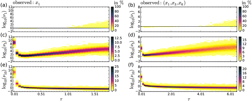
Figure 1: (Color online) Probability distributions (color coded frequency in %, vertically plotted) of uncertainties $\nu_{1}$, $\nu_{5}$ and $\nu_{10}$ vs. delay time $\tau$ for the Lorenz-96 model. The uncertainties $\nu_{1}$ and $\nu_{5}$ correspond to state variables $x_{1}$ and $x_{5}$, respectively, and $\nu_{10}$ corresponds to the parameter $p$. In the left column ((a),(c),(e)) a scalar ($L=1$ dimensional) measurement function $h(\mathbf{x}(t))=x_{1}(t)$ is used for generating delay coordinates with $K=12$. The right column ((b),(d),(f)) shows results for the $L=3$ dimensional measurement function $\mathbf{h}(\mathbf{x}(t))=(x_{1}(t),x_{3}(t),x_{6}(t))$ and a delay reconstruction (Eq. (6)) with $K=4$. Hence $D_{M}=12$ dimensional delay coordinates (Eq. (6)) are constructed in both cases. The histograms for $\nu_{1}$ are very similar to histograms obtained for other measured state variables ($x_{3}$, $x_{6}$ in the right column), not shown here. Similarly, the histograms of $\nu_{5}$ are representative for histograms of the remaining unmeasured state variables (not shown here).

The left column shows the results for $h(\mathbf{x}(t))=x_{1}(t)$ and the right column for $\mathbf{h}(\mathbf{x}(t))=(x_{1}(t),x_{3}(t),x_{6}(t))$. In both cases the uncertainty $\nu_{1}$ corresponds to the “measured” state variable $x_{1}$, $\nu_{5}$ corresponds to the “hidden” state variable $x_{5}$ (not measured directly), and $\nu_{10}$ corresponds to the model parameter $p$. Histograms for the other $\nu_{i}$ are not shown, because they look very similar to the histograms for $\nu_{1}$ (if the corresponding state variable is measured) and $\nu_{5}$ (if the corresponding model state variable is unmeasured). The reason for these similarities is the symmetry in the Lorenz-96 model equations (3).

For both measurement functions one can see that the uncertainty values of the maxima of the histograms exhibit a U-shaped dependence on the delay time $\tau$. The smallest uncertainties occur between $\tau=0.11$ and $\tau=0.21$ for the unmeasured state variables (Figs. 1c,d). In both cases the distribution of the uncertainty $\nu_{1}$ of the measured state variable (and similar for $\nu_{3}$ and $\nu_{6}$ if $R=3$, not shown) possess a sharp peak around $\log_{10}\nu_{i}=0$. In this case the state variable $x_{1}$ is an observed quantity, and therefore, the delay reconstruction does not provide much further information about its values. For relatively large delay times ( $\tau>1$ in (a) and $\tau>4$ in (b)) the delay reconstruction becomes rather “poor”. The measurement noise is amplified resulting in a tail of the histogram with uncertainty values larger than one (the yellow areas above the horizontal line at $\log(\nu_{1})=0$). This result is not surprising, because in nonlinear time series analysis it is well known that the delay time has to be chosen carefully and must not be too large for chaotic attractors, since otherwise the reconstructed attractor will be heavily distorted. In contrast, the $\nu$-values of the centers of the distributions of the uncertainty $\nu_{10}$ of the parameter $p$ decrease with increasing $\tau$ until the maximum of the distribution is below one (see Figs. 1e,f) (without exhibiting a clear minimum).

As mentioned before, these two examples are representative for all multivariate time series from the Lorenz-96 model consisting of combinations of one to three state variables. The other 13 combinations show similar histograms. If a certain state variable in one of the other combinations is measured, then the corresponding histogram of the corresponding uncertainty looks similar to the histograms of $\nu_{1}$ in Fig. 1a. The same holds for state variables that are not contained in the multivariate time series (and where the corresponding $\nu$ histograms look similar to the histograms of $\nu_{5}$ in Fig. 1) and the model parameter $p$ (the corresponding $\nu_{10}$ histograms look similar to the histograms of $\nu_{10}$ in Fig. 1). With an increasing number of measured state variables (from one to three) the maxima of the distributions at the minimum of the histograms of $\nu$ for unmeasured state variables move only slightly in the direction of smaller $\nu$ (see, for example, Figs. 1c,d). This trend also holds for all combinations of four measured state variables (not shown here). The fact that the histograms for one to three observed state variables look almost the same means that the local observability of the model parameter and the unmeasured state variables is maintained, even if only a single model state variable is measured instead of three (or more). In the following we shall investigate whether this local result holds for states that are not close to the true solution. Specifically, we want to know if we can uniquely recover the true solution using a univariate time series (from a single observable), even if the initial guesses are far from the true solution. Since the true solution is a stable fixed point of any optimization based estimation algorithm, we are thus interested in the ’size’ and the structure of the basin of attraction of this fixed point. To address this question we shall introduce in the next section a particular estimation algorithm which is used herev as a prototypical example for investigating the solution basin.

IV State and Parameter estimation algorithm

The method used in this study to adapt a model to a time series is based on minimizing a cost function and in the context of this paper it represents only one out of many different state and parameter estimation methods CGA08 ; B10 where the same type of basin size analysis could be applied. The method was introduced in Ref. SBP11 and will be summarized in the following.

The goal of the estimation process is to find a set of values for the model state variables $\mathbf{x}(t)$ at each time step of its discretization and the model parameters $\mathbf{p}$ such that the model equations, given by a set of ODEs (see Eq. (1)), provide via the measurement function (2) a model times series $\{\mathbf{y}(n)\}$ consisting of $N+1$ samples $\mathbf{y}(n)\hat{=}\mathbf{y}(t_{n})\in\mathbb{R}^{L}$ with $t_{n}\in{\cal{T}}\,\forall\,n$ that matches the experimental time series $\{\bm{\eta}(n)\}$. In other words, the average difference between $\bm{\eta}(n)$ and $\mathbf{y}(n)$ should be small.

Furthermore, the model equations should be fulfilled as well as possible. This means that modeling errors $\mathbf{u}(t)$ are allowed, but should be small. Therefore, model (1) is extended to include modeling errors $\mathbf{u}(t)$,

$$\frac{\mathrm{d}\mathbf{x}(t)}{\mathrm{d}t} =\mathbf{F}(\mathbf{x}(t),\mathbf{p},t)+\mathbf{u}(t)\,,$$ (8)

so that when $\mathbf{u}(t)$ is small the model trajectory $\mathbf{x}(t)$ closely matches the model equations. To incorporate model error into the optimization, we discretize $\mathbf{u}(t)$ and $\mathbf{x}(t)$ at times $t_{n}\in{\cal{T}}$ so that the state variables $\{\mathbf{x}(n)\}$, $\mathbf{x}(n)\hat{=}\mathbf{x}(t_{n})$, at each time $n$ must be estimated in addition to $\mathbf{p}$. For simplicity, we choose $\mathbf{x}(t)$ and $\mathbf{y}(t)$ to be sampled at the same times that the data are observed. Similarly, $\mathbf{u}(t)$ is discretized to $\{\mathbf{u}(n)\}$ with $\mathbf{u}(n)\hat{=}\mathbf{u}(t_{n})$ and $t_{n}\in{\cal{T}}$. The discretization of (8) is given by

$$\mathbf{u}(n) \approx\left.\frac{\Delta\mathbf{x}}{\Delta t}\right|_{t_{n}}-\mathbf{F}(\mathbf{x}(n),\mathbf{p},t_{n})\,,$$ (9)

where the symbol $\left.\frac{\Delta\mathbf{x}}{\Delta t}\right|_{t_{n}}$ stands for the finite difference approximation of $\frac{\mathrm{d}\mathbf{x}(t)}{\mathrm{d}t}$ at time $t_{n}$.

The goal of the adaption process is to minimize (on average) the norm of $\mathbf{u}(n)$ and the norm of the difference $\bm{\eta}(n)-\mathbf{y}(n)$ for all $n\in{\cal{T}}$. Technically, this optimization problem can be implemented in different ways ACFK09 and in the following we use unconstrained optimization SBP11 employing automatic differentiation SBLP13 . The cost function used in this study can be derived from a general probabilistic description of the estimation problem assuming Gaussian distributions (also called weakly constrained 4D-VAR in geosciences) E97 ; LE96 ; QA10 ; Evensen09 and consists of four terms

$$C(\{\mathbf{x}(n)\},\mathbf{p}) =C_{1}+C_{2}+C_{3}+C_{4}$$ (10)

with

$$C_{1} =\frac{\alpha}{N+1}\cdot\sum_{n=0}^{N}\left(\bm{\eta}(n)-\mathbf{y}(n)\right)^{\mathrm{tr}}\mathbf{A}\left(\bm{\eta}(n)-\mathbf{y}(n)\right)$$ (11)

$$C_{2} =\frac{1-\alpha}{N+1}\cdot\sum_{n=0}^{N}\mathbf{u}(n)^{\mathrm{tr}}\mathbf{B}\mathbf{u}(n)$$ (12)

$$C_{3} =\frac{1-\alpha}{N+1}\cdot\sum_{n=3}^{N-2}\left(\mathbf{x}_{\mathrm{apr}}(n)-\mathbf{x}(n)\right)^{\mathrm{tr}}\mathbf{E}\left(\mathbf{x}_{\mathrm{apr}}(n)-\mathbf{x}(n)\right)$$ (13)

$$C_{4} =\beta\cdot\mathbf{q}(\mathbf{w},\mathbf{w}_{\mathrm{l}},\mathbf{w}_{\mathrm{u}})^{\mathrm{tr}}\cdot\mathbf{q}(\mathbf{w},\mathbf{w}_{\mathrm{l}},\mathbf{w}_{\mathrm{u}})\,.$$ (14)

The term $C_{1}$ penalizes the difference between $\bm{\eta}(n)$ and $\mathbf{y}(n)$ whereas $C_{2}$ penalizes large magnitudes of $\mathbf{u}(n)$. In the term $C_{3}$ a Hermite interpolation is performed to determine $\mathbf{x}_{\mathrm{apr}}(n)$ from neighboring points and the time derivatives which are, according to (8), given by $\mathbf{F}(\mathbf{x}(t),\mathbf{p},t)+\mathbf{u}(t)$ and provide the approximate solutions

$$\mathbf{x}_{\mathrm{apr}}(n)= \frac{11}{54}\left[\mathbf{x}(n-2)+\mathbf{x}(n+2)\right]+\frac{8}{27}\left[\mathbf{x}(n-1)\right.$$

$$\left.+\mathbf{x}(n+1)\right]+\frac{\Delta t}{18}\left[\mathbf{F}(\mathbf{x}(n-2),\mathbf{p},t_{n-2})\right.$$

$$\left.+\mathbf{u}(t_{n-2})-\mathbf{F}(\mathbf{x}(n+2),\mathbf{p},t_{n+2})-\mathbf{u}(t_{n+2})\right]$$

$$+\frac{4\Delta t}{9}\left[\mathbf{F}(\mathbf{x}(n-1),\mathbf{p},t_{n-1})+\mathbf{u}(t_{n-1})\right.$$

$$\left.-\mathbf{F}(\mathbf{x}(n+1),\mathbf{p},t_{n+1})-\mathbf{u}(t_{n+1})\right]\,.$$ (15)

Smoothness of $\{\mathbf{x}(n)\}$ is enforced by small differences $\mathbf{x}_{\mathrm{apr}}(n)-\mathbf{x}(n)$. The term $C_{3}$ suppresses non-smooth (oscillating) solutions which may occur without this term in the cost function. In this paper the weight matrices $\mathbf{A}$, $\mathbf{B}$ and $\mathbf{E}$ are diagonal matrices. The diagonal elements can be used for an individual weighting.

The solution $(\{\hat{\mathbf{x}}(n)\},\hat{\mathbf{p}})$ obtained through the optimization of the cost function (10) is taken to be the maximum likelihood estimate.

Let

$$\mathbf{w} =(\{\mathbf{x}(n)\},\mathbf{p})$$ (16)

be a vector containing all quantities to be estimated. To force $\mathbf{w}$ to stay between the lower and upper bounds $\mathbf{w}_{\mathrm{l}}$ and $\mathbf{w}_{\mathrm{u}}$, respectively, the vector valued function $\mathbf{q}(\mathbf{w},\mathbf{w}_{\mathrm{l}},\mathbf{w}_{\mathrm{u}})=(q_{1},\dots,q_{L})^{\mathrm{tr}}$ is defined as

$$q_{i}(w_{i},w_{\mathrm{l},i},w_{\mathrm{u},i}) =\begin{cases}w_{\mathrm{u},i}-w_{\mathrm{i}}&\mathrm{for}\enskip w_{i}\geq w_{\mathrm{u},i}\\ 0&\mathrm{for}\enskip w_{\mathrm{l},i}<w_{\mathrm{i}}<w_{\mathrm{u},i}\\ w_{\mathrm{l},i}-w_{\mathrm{i}}&\mathrm{for}\enskip w_{i}\leq w_{\mathrm{l},i}.\\ \end{cases}$$ (17)

$q_{i}$ is zero if the value of $w_{i}$ lies within its bounds. To enforce this, the positive parameter $\beta$ is set to a large number, e.g. $10^{5}$.

The homotopy parameter $\alpha$ can be used to control whether the solution should be close to data ($\alpha\approx 1$) or has a smaller error in fulfilling the model equations. In Ref. BS11 a technique is described to find an optimal $\alpha$. Furthermore, one might use continuation (see Ref. B10 ) where $\alpha$ is stepwise decreased. Starting with $\alpha\approx 1$ results in a solution close to the data. Then, $\alpha$ is slightly decreased and the previously obtained solution is used as an initial guess to optimize the cost function again. This procedure is repeated until the value $\alpha=0.5$ is reached.

Note that the cost function can be written in the form

$$C(\mathbf{w})=\sum_{j=1}^{J}H_{j}(\mathbf{w})^{2}=\left\|\mathbf{H}(\mathbf{w})\right\|_{2}^{2}$$ (18)

where $\mathbf{H}(\mathbf{w})$ is a high dimensional vector valued function of the high dimensional vector $\mathbf{w}$. To optimize (18) we use an implementation of the Levenberg-Marquardt algorithm L44 ; M63 called sparseLM sparseLM . Although $C(\mathbf{w})$ will be optimized, sparseLM requires $\mathbf{H}(\mathbf{w})$ and the sparse Jacobian of $\mathbf{H}(\mathbf{w})$ as input which is computed using the automatic differentiation tool ADOL-C adolc ; GJU96 , and described in more detail in SBLP13 .

V Determining the basin size of the true solution

In Sec. IV we described a state and parameter estimation algorithm that has to be initialized with guesses for all model state variables $\mathbf{x}(t_{n})$ at each time step $t_{n}$ and all fixed model parameters $\mathbf{p}$. This set of values forms an initial guess, which must be supplied to the optimization algorithm. In this section three different methods for generating the initial guesses are presented and simulations consisting of twin experiments are performed to determine which of these methods gives the best estimates for the model state variables and fixed parameters. These estimates are then compared with the true solution which is known exactly in this case since this is a twin experiment. Due to the fact that the methods for generating the initial guesses, in a certain way, depend on random numbers and the outcome of an estimation process is either successful (estimated states and parameters are close to the ones used to generate the data time series) or not successful (estimated states and parameters are not close to the ones used to generate the data time series) the simulations can be considered as Bernoulli experiments and the basin size of initial guesses leading to the true solution can be determined, as suggested by Menck et al. MHMK13 in another context.

V.1 The simulation

First we generate 18 “true” trajectories $\{^{i}\mathbf{z}(n)\}$ with $i=1,\dots,18$ by integrating the 9-dimensional Lorenz-96 model (3) with 18 different initial conditions $\mathbf{z}(0)$ on the attractor with $\Delta t=0.01$ and $N=1500$ using the model parameter $p=8.17$. Then $N_{\mathrm{iguess}}=500$ initial guesses $(\{{}_{h}^{i}\mathbf{x}(n)\},{}_{h}p)$ ($h=1,\dots,N_{\mathrm{iguess}}$) of the model state variables and the (fixed) parameter $p$ are generated which are used for initializing the estimation procedure (the estimation algorithm was described in Sec. IV). Three different methods for generating the initial guesses will be presented in Sec. V.2. The following steps in the simulation do not depend on the specific choice of the method for creating the initial guesses.

From each of the 18 true trajectories $\{^{i}\mathbf{z}(n)\}$ with $i=1,\dots,18$, according to Sec. II, 15 multivariate time series were extracted corresponding to the 15 different combinations of state variables assumed to measured. This gives 270 different multivariate time series with one, two, or three state variables:

$$\{{}^{i}z_{1}(n)\},\{{}^{i}(z_{1}(n),z_{2}(n))\},\{{}^{i}(z_{1}(n),z_{3}(n))\},$$

$$\{{}^{i}(z_{1}(n),z_{4}(n))\},\{{}^{i}(z_{1}(n),z_{5}(n))\},$$

$$\{{}^{i}(z_{1}(n),z_{2}(n),z_{3}(n))\},\{{}^{i}(z_{1}(n),z_{2}(n),z_{4}(n))\},$$

$$\{{}^{i}(z_{1}(n),z_{2}(n),z_{5}(n))\},\{{}^{i}(z_{1}(n),z_{2}(n),z_{6}(n))\},$$

$$\{{}^{i}(z_{1}(n),z_{2}(n),z_{7}(n))\},\{{}^{i}(z_{1}(n),z_{2}(n),z_{8}(n))\},$$

$$\{{}^{i}(z_{1}(n),z_{3}(n),z_{5}(n))\},\{{}^{i}(z_{1}(n),z_{3}(n),z_{6}(n))\},$$

$$\{{}^{i}(z_{1}(n),z_{3}(n),z_{7}(n))\},\{{}^{i}(z_{1}(n),z_{4}(n),z_{7}(n))\}$$ (19)

with $i=1,\dots,18$, $\Delta t=0.01$, $n=0,1,\dots,N$ and $N=1500$.

To make the simulation more realistic, white noise (normally distributed random numbers) is added to these 270 clean, multivariate times series. This results in 270 noisy multivariate time series $\{{}^{i}\bm{\eta}^{c}(n)\}$ with $\Delta t=0.01$, $n=0,1,\dots,N$ and $N=1500$.

Each noisy time series is computed by

$${}^{i}\bm{\eta}^{c}(n) =\mathbf{h}^{c}\left({}^{i}\mathbf{z}(n)\right)+\sigma_{\mathrm{ts}}{}^{i}\mathbf{\xi}^{c}(n)\,,$$ (20)

where $\sigma_{\mathrm{ts}}=0.2$ and ${}^{i}\mathbf{\xi}^{c}(n)=\left({}^{i}\mathbf{\xi}^{c}_{1}(n),\dots,{}^{i}\mathbf{\xi}^{c}_{L}(n)\right)\in\mathbb{R}^{L}$ are independent, normally distributed random variables with zero mean and a variance of one, ${}^{i}\mathbf{\xi}^{c}_{l}(n)\sim\mathcal{N}(0,1)$.

The index $i=1,\dots,18$ describes the true trajectory $\{{}^{i}\mathbf{z}(n)\}$ from which the data time series was extracted. Index $c$ indicates which state variables were measured. For example, $c=\mathrm{(1-2-6)}$ means that the state variables $z_{1}$, $z_{2}$ and $z_{6}$ are the measured state variables. The label $h=1,\dots,N_{\mathrm{iguess}}$ describes with which initial guess the estimation algorithm was initialized. The measurement function $\mathbf{h}^{c}(\mathbf{x}(t))$ is always chosen according to the measured state variables defined by $c$. If, for example, the state variables $z_{1},z_{2}$ and $z_{7}$ are measured (and therefore $c=1-2-7$), then the measurement function is given by $\mathbf{h}^{c}(\mathbf{x}(t))=(x_{1}(t),x_{2}(t),x_{7}(t))$.

To each of the 270 multivariate time series $\{{}^{i}\bm{\eta}^{c}(n)\}$ the Lorenz-96 model is adapted $N_{\mathrm{iguess}}=500$ times, whereas each of the $N_{\mathrm{iguess}}$ estimation processes is initialized with one of the previously generated $N_{\mathrm{iguess}}$ different (random) initial guesses using the estimation algorithms described in Sec. IV. This means that $N_{\mathrm{iguess}}\cdot 270=500\cdot 270=135000$ estimation problems are solved.

For each solution of the estimation processes the difference between the true and the estimated solution is given by the estimation error

$${}_{h}^{i}E^{c}= \frac{1}{(N+1)\cdot D}\sum_{n=0}^{N}\left\|{}^{i}\mathbf{z}(n)-{}_{h}^{i}\hat{\mathbf{x}}^{c}(n)\right\|^{2}_{2}\,.$$ (21)

The indices of ${}_{h}^{i}E^{c}$, ${}^{i}\mathbf{z}^{c}(n)$ and ${}_{h}^{i}\hat{\mathbf{x}}^{c}(n)$ have the same meaning as for $\{{}_{h}^{i}\hat{\mathbf{x}}^{c}(n)\}$. The smaller the error measure ${}_{h}^{i}E^{c}$ the closer the estimated solution for the model state variables is to the true solution and hence the more accurately the estimation problem was solved. The estimation of state variables is considered as successful if ${}_{h}^{i}E^{c}<10^{-2}$, else the estimation is considered as not successful. The value for the estimated fixed model parameter ${}_{h}^{i}\hat{p}^{c}$ is considered as successful, if ${}_{h}^{i}\hat{p}^{c}\in[8.16,8.18]$ (remember, the true trajectories $\{{}^{i}\hat{\mathbf{z}}(n)\}$ were generated with $p=8.17$ in Eq. (3)).

We are interested in a quantity (in percentage) which tells us how many estimations with a specific true trajectory, $i$, and a specific combination of observed state variables, $c$, of the model state variables are successful. In other words: For how many of the $N_{\mathrm{iguess}}=500$ estimations using $N_{\mathrm{iguess}}$ different initial guesses with a specific true trajectory, $i$, and a specific combination of observed state variables, $c$, is the estimation of the model state variables successful, i.e. ${}_{h}^{i}E^{c}<10^{-2}$? This quantity, which of course depends on the true trajectory and the combination of measured state variables, is defined here as the success rate of the estimation of the model state variables (in percentage)

$$\left<{}^{i}E^{c}\right> =\frac{100\%}{N_{\mathrm{iguess}}}\sum_{h=1}^{N_{\mathrm{iguess}}}e_{h},$$ (22)

$$\mathrm{with}\quad e_{h} =\left\{\begin{matrix}0,&\mathrm{if}\;{}_{h}^{i}E^{c}>10^{-2}\\ 1,&\mathrm{if}\;{}_{h}^{i}E^{c}\leq 10^{-2}\end{matrix}\right.\;.$$

One can also define an error which depends on the estimated solution and the data, only, as

$${}_{h}^{i}E^{c}_{\mathrm{obs}}= \frac{1}{(N+1)\cdot L}\sum_{n=0}^{N}\left\|{}^{i}\bm{\eta}^{c}(n)-\mathbf{h}^{c}\left({}_{h}^{i}\hat{\mathbf{x}}^{c}(n)\right)\right\|^{2}_{2}\;.$$ (23)

Assume one estimates the best possible solution. That is, if the estimated solution is equal to the trajectory (without noise) used to generate the data, ${}_{h}^{i}\hat{\mathbf{x}}^{c}(n)={}^{i}\mathbf{z}(n)$. In this case Eq. (23) is (using eq. (20))

$${}_{h}^{i}E^{c}_{\mathrm{obs,opt}}= \frac{1}{(N+1)L}\sum_{n=0}^{N}\left\|{}^{i}\bm{\eta}^{c}(n)-\mathbf{h}^{c}\left({}^{i}\mathbf{z}^{c}(n)\right)\right\|^{2}_{2}$$

$$= \frac{\sigma_{\mathrm{ts}}^{2}}{(N+1)L}{}^{i}Q^{c}\;,$$ (24)

where

$${}^{i}Q^{c}= \sum_{n=0}^{N}\sum_{l=1}^{L}\left[{}^{i}\xi^{c}_{l}(n)\right]^{2}\;.$$ (25)

Because ${}^{i}\xi^{c}_{l}(n)$ are independent, standard normal random variables, ${}^{i}Q^{c}$ is chi-squared distributed, ${}^{i}Q^{c}\sim\chi^{2}_{(N+1)L}$, with $(N+1)L$ degrees of freedomnumerical_recipes_2007 . The expectation value is then given by $E\left[{}^{i}Q^{c}\right]=(N+1)L$, leading to an expectation value for ${}_{h}^{i}E^{c}_{\mathrm{obs,opt}}$ of

$$E\left[{}_{h}^{i}E^{c}_{\mathrm{obs,opt}}\right] =\sigma_{\mathrm{ts}}^{2}\;.$$ (26)

The variance of the chi-square distribution is $\operatorname{Var}\left[{}^{i}Q^{c}\right]=2(N+1)L$. The variance of ${}_{h}^{i}E^{c}_{\mathrm{obs,opt}}$ is then

$$\operatorname{Var}\left[{}_{h}^{i}E^{c}_{\mathrm{obs,opt}}\right] =\operatorname{Var}\left[\frac{\sigma_{\mathrm{ts}}^{2}}{(N+1)L}{}^{i}Q^{c}\right]$$

$$=\frac{\sigma_{\mathrm{ts}}^{4}}{[(N+1)L]^{2}}\operatorname{Var}\left[{}^{i}Q^{c}\right]$$

$$=\frac{2\sigma_{\mathrm{ts}}^{4}}{(N+1)L}$$ (27)

giving the standard deviation

$$\operatorname{Std}\left[{}_{h}^{i}E^{c}_{\mathrm{obs,opt}}\right] =\sqrt{\operatorname{Var}\left[{}_{h}^{i}E^{c}_{\mathrm{obs,opt}}\right]}$$

$$=\sigma_{\mathrm{ts}}^{2}\sqrt{\frac{2}{(N+1)L}}\;.$$ (28)

As described in Sec. V.1 we use $\sigma_{\mathrm{ts}}=0.2$ and $N=1500$. For one observed state variable, $L=1$, and a perfect solution of the estimation problem, we get the lower boundary for ${}_{h}^{i}E^{c}_{\mathrm{obs}}$, Eq. (23), of

$$\sigma_{\mathrm{ts}}^{2}\left[1\pm\sqrt{\frac{2}{(N+1)L)}}\right]\approx 0.04\pm 0.00146\;.$$ (29)

Note that only the standard deviation depends on the number of measurements (and is largest for $L=1$), but not the expectation value. This means that with a smooth estimate for the model state variables one can not go below this boundary. If one goes below this threshold, the measurement noise is modelled and one has not estimated a smooth solution for the model variables. In this case one should choose a smaller $\alpha$ in the cost function Eq. (10). Note that the modelling of the measurement noise is still possible if one does not fall below this boundary. Because of the perfect model scenario in our twin experiments we can expect a value for ${}_{h}^{i}E^{c}_{\mathrm{obs}}$ which is only slightly larger (due to small numerical errors) than the lower boundary of $0.04\pm 1.46\cdot 10^{-3}$. To cover these cases we introduce an empirical margin of 0.005 which is added to the lower bound of 0.04 and we consider an estimation as successful if ${}_{h}^{i}E^{c}_{\mathrm{obs}}\leq 0.045$. Applying this bound to the error given by Eq. (23) we can define a success rate (in percentage)

$$\left<{}^{i}E_{\mathrm{obs}}^{c}\right> =\frac{100\%}{N_{\mathrm{iguess}}}\sum_{h=1}^{N_{\mathrm{iguess}}}e_{h},$$ (30)

$$\mathrm{with}\quad e_{h} =\left\{\begin{matrix}0,&\mathrm{if}\;{}_{h}^{i}E_{\mathrm{obs}}^{c}>0.045\\ 1,&\mathrm{if}\;{}_{h}^{i}E_{\mathrm{obs}}^{c}\leq 0.045\end{matrix}\right.\;.$$

In a similar way, the success rate of the estimation of the model parameter (in percentage) ${}_{h}^{i}\hat{p}^{c}$ is defined as

$$\left<{}^{i}\hat{p}^{c}\right> =\frac{100\%}{N_{\mathrm{iguess}}}\sum_{h=1}^{N_{\mathrm{iguess}}}p_{h},$$ (31)

$$\mathrm{with}\quad p_{h} =\left\{\begin{matrix}0,&\mathrm{if}\;{}_{h}^{i}\hat{p}^{c}\notin[8.16,8.18]\\ 1,&\mathrm{if}\;{}_{h}^{i}\hat{p}^{c}\in[8.16,8.18]\end{matrix}\right.\;.$$

Note, that in a real world experiment ${}_{h}^{i}E^{c}$, and hence $\left<{}^{i}E^{c}\right>$, typically can not be computed due to the unknown true trajectory $\{{}^{i}\mathbf{z}(n)\}$. Another possibility to compute the accuracy of the estimated model state variables and the fixed model parameters is to compare predictions of the model via the measurement function $\mathbf{h}(\mathbf{x}(t))$, Eq. (2), with available (noisy) data after the estimation window. To compute the prediction the model Eq. (1) must be integrated starting at the end of the estimation window at $t_{N}$ using the estimated value ${}_{h}^{i}\hat{p}^{c}$ as model parameter and ${}_{h}^{i}\hat{\mathbf{x}}^{c}(N)$ as initial guesses. Next, the prediction $\{{}_{h}^{i}\mathbf{x}^{c}(n)\}$, $n\geq N$, can be compared with observed data $\{{}^{i}\bm{\eta}^{c}(n)\}$, $n\geq N$, by computing the prediction error

$${}_{h}^{i}\mathrm{PE}^{c}= \frac{1}{(N_{\mathrm{pred}}+1)\cdot L}\sum_{n=N}^{N+N_{\mathrm{pred}}}\left\|{}^{i}\bm{\eta}^{c}(n)-\mathbf{h}^{c}\left({}_{h}^{i}\mathbf{x}^{c}(n)\right)\right\|^{2}_{2}$$ (32)

for $N_{\mathrm{pred}}$ time steps using the same step size $\Delta t$ as for computing the true trajectories. Due to noise in the data the prediction error cannot vanish and we consider a prediction as successful, if ${}_{h}^{i}\mathrm{PE}^{c}<0.5$. Analogous to Eq. (22) we define the success rate of the prediction (in percentage)

$$\left<{}^{i}\mathrm{PE}^{c}\right> =\frac{100\%}{N_{\mathrm{iguess}}}\sum_{h=1}^{N_{\mathrm{iguess}}}\mathrm{pe}_{h},$$ (33)

$$\mathrm{with}\quad\mathrm{pe}_{h} =\left\{\begin{matrix}0,&\mathrm{if}\;{}_{h}^{i}\mathrm{PE}^{c}>0.5\\ 1,&\mathrm{if}\;{}_{h}^{i}\mathrm{PE}^{c}\leq 0.5\end{matrix}\right.$$

describing for how many of the different initial guesses with the same true trajectory and the same combination of measured state variables the prediction was successful. In contrast to ${}_{h}^{i}E^{c}$ the prediction error ${}_{h}^{i}\mathrm{PE}^{c}$ can be computed using measured data only.

V.2 Different methods for generating initial guesses

For the optimization process initial guesses for the model state variables and the fixed model parameter $p$ have to be chosen. In our simulation we considered three methods for preparing initial guesses according to rules specified below. For each case $N_{\mathrm{iguess}}=500$ different guesses $(\{{}_{h}^{i}\mathbf{x}(n)\},{}_{h}p)$ with $h=1,\dots,N_{\mathrm{iguess}}$ are generated. In all three cases the model parameter ${}_{h}p$ is picked equally distributed from the interval $[4,20]$. In those cases where the initial guess $\{{}_{h}^{i}\mathbf{x}(n)\}$ for the model state variables does not depend on the true trajectory $\{{}^{i}\mathbf{z}(n)\}$ of the estimation problem, the index $i$ will be neglected (i.e. ${}_{h}^{i}\mathbf{x}(n)={}_{h}\mathbf{x}(n)$). In the following, three different methods of choosing the initial guesses will be used and evaluated:

1. Uniformly distributed samples in a box: For each initial guess each model state variable ${}_{h}x_{d}(n)$, $d=1,\dots,D$ at each time step $t_{n}$ is an equally distributed random number in the interval $[-9,14]$. This interval has been chosen because it is the range of typical oscillations of all state variables of the Lorenz-96 model. Together with the model parameter the initial guesses consist of $D\cdot N+1=D_{\mathrm{iguess}}=13501$ numerical values. In other words, the initial guesses are uniformly distributed points in a box in a $D_{\mathrm{iguess}}$ dimensional space $\mathbb{R}^{D_{\mathrm{iguess}}}$.

2. Exact solutions of the model: Each initial guess $(\{{}_{h}\mathbf{x}(n)\},{}_{h}p)$ is an exact solution of the Lorenz-96 model Eq. (3). The initial values ${}_{h}\mathbf{x}(0)$ of these trajectories are arbitrary points on the attractor generated with $p=8.17$ (not coinciding with the initial conditions of the true trajectories).

3. Samples close to the true solution: These initial guesses depend, in contrast to methods 1 and 2, on the “true trajectories” $\{{}^{i}\mathbf{z}(n)\}$ with $i=1,\dots,18$ (see Sec. V.1). The estimation processes will be initialized with a “noisy” version of $\{{}^{i}\mathbf{z}(n)\}$. More precisely, for each time step $t_{n}$ uniformly distributed random numbers from the interval $[-15,15]$ are added to the values of the true state $\{{}^{i}\mathbf{z}(n)\}$ to generate the initial guesses $\{{}_{h}^{i}\mathbf{x}(n)\}$, Compared to initial guess strategy 1 and 2 this strategy does depend on the true trajectories. In a real world application, where the true trajectories are not known, this strategy can not be used in contrast to methods 1 and 2.

V.3 Interpretation of the simulation as Bernoulli experiment and error estimation

As described in Sec. V.1 for each of the 18 true trajectories and each of the 15 combinations of measured state variables, the Lorenz-96 model was adapted $N_{\mathrm{iguess}}=500$ times to the corresponding (multivariate) time series using a specific method for choosing the initial guesses. If ${}_{h}^{i}E^{c}<10^{-2}$ (Eq. (21)) then the estimation of the model state variables is considered as successful. This simulation can be interpreted as a Bernoulli experiment, because each of the independent $N_{\mathrm{iguess}}$ estimations of the model state variables and the fixed parameter is a Bernoulli trial with the outcome successful or not successful. The standard error of the Bernoulli process is given by

$${}^{i}e^{c} :=\frac{\sqrt{{}^{i}p^{c}(100\%-{}^{i}p^{c})}}{\sqrt{N_{\mathrm{iguess}}}}\,,$$ (34)

whereas ${}^{i}p^{c}\in[0\%,100\%]$ is the expectation value of the percentage of successful cases (index $i$ describes the used true trajectory and index $c$ describes the combination of measured state variables). Unfortunately, we do not know ${}^{i}p^{c}$. However, we can determine the maximum of the standard error ${}^{i}e^{c}$ which occurs for ${}^{i}p^{c}=50\%$. With $N_{\mathrm{iguess}}=500$ trials the maximal standard error equals ${}^{i}e^{c}_{\mathrm{max}}\approx 2.24\%$ and hence is sufficiently small.

V.4 Results

V.4.1 Estimation Error

The simulation described in Sec. V.1 was performed with all three methods for choosing initial guesses for the model state variables and the fixed model parameters $(\{{}_{h}^{i}\mathbf{x}(n)\},{}_{h}p)$ as described in Sec. V.2. For each method of choosing the initial guesses the percentage of successful estimations, $\left<{}^{i}E^{c}\right>$, Eq. (22), was computed, where an estimation of the model state variables is considered as successful if ${}_{h}^{i}E^{c}<10^{-2}$, Eq. (21) (see Sec. V.1). The estimation of the model parameter is considered as successful if ${}_{h}^{i}\hat{p}^{c}\in[8.16,8.18]$. The success rate for the fixed model parameter, $\left<{}^{i}\hat{p}^{c}\right>$, is defined in Eq. (31). The statistic (percentage of successful estimations) was created for each of the 18 true trajectories $\{^{i}\mathbf{z}(n)\}$ (indexed by $i$), each of the 15 combinations of observed state variables, $c$, and all $N_{\mathrm{iguess}}=500$ initial guesses (indexed by $h$).

Tables 1a,b show the results for method 1 (uniformly distributed samples in a box). The tables show $\left<{}^{i}E^{c}\right>$ (Table 1a) and $\left<{}^{i}\hat{p}^{c}\right>$ (Table 1b) for each combination of a true trajectory $\{^{i}\mathbf{z}(n)\}$ and a particular choice of measured state variables. If three variables are measured, the rate of successful estimations of the model variables and the fixed parameter is (on average) higher for all combinations of measured state variables compared to the success rate for multivariate time series with only two variables.

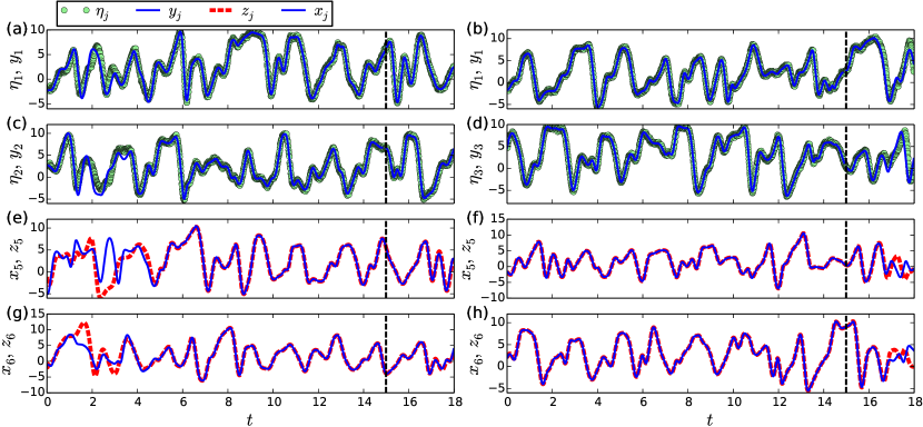
Figure 2: This figure show two examples where the Lorenz-96 model Eq. (3) was adapted to a (multivariate) time series $\eta_{j}$. The (unmeasured) model state variables $x_{j}$ and the fixed model parameter were estimated using the estimation method 1 described in Sec. IV. The output of the measurement function is $y_{j}$ and the true trajectory is $z_{j}$ (unknown to the estimation algorithm). The estimation was performed for $0<t<15$ and the prediction of the model variables for $15\leq t<18$ (right of the vertical black dashed line at $t=15$). Left column, (a), (c), (e), (g): $x_{1}$ and $x_{2}$ are measured ($c=\mathrm{(1-2)}$) and $i=3$, $h=385$. The estimation error of model variables is larger than the prediction error, ${}_{385}^{3}E^{\mathrm{(1-2)}}=1.73>{}_{385}^{3}\mathrm{PE}^{\mathrm{(1-2)}}=0.054$. Right column, (b), (d), (f), (h): $x_{1}$ and $x_{3}$ are measured ($c=\mathrm{(1-3)}$) and $i=1$, $h=140$. The estimation error of model variables is smaller than the prediction error, ${}_{140}^{1}E^{\mathrm{(1-3)}}=6.1\cdot 10^{-4}<{}_{140}^{1}\mathrm{PE}^{\mathrm{(1-3)}}=1.98$.

Nevertheless, certain combinations with two observed variables $(x_{1},x_{2})$, $(x_{1},x_{3})$ or $(x_{1},x_{4})$ also give success rates that are only slightly lower than combinations of three observed state variables. They just appear less often compared to time series with three observed state variables. When $(x_{1},x_{5})$ are observed the estimation of the model state variables and the fixed parameter does not seem to work very well. None of the 18 trajectories considered here exhibit high success rate. If only $x_{1}$ is observed the estimation of variables and the parameter fails for all 18 trajectories. As one might expect, one can see a high correlation between the success rate for the state variable estimation (Tab. 1a) and the success rate for the parameter estimation (Tab. 1b). The success rates depend not only on the combination of observed variables only, but also on the trajectory $\{^{i}\mathbf{z}(n)\}$ used to generate the time series (i.e. the starting points on the attractor).

In Tab. 2 the success rate of the error defined by Eq. (30) is shown. Compared to Eq. (22) this success rate can be computed from the data and the estimated model state variables only. One can see a high correlation between Tab. 1a and Tab. 2 indicating that ${}_{h}^{i}E^{c}_{\mathrm{obs}}$ is a good approximation of ${}_{h}^{i}E^{c}$ (at least in the absence of errors in the model equations, as in these simulations). There are, however, some discrepancies. For example, if $\{{}^{5}\mathbf{z}(n)\}$ is the true trajectory and $c=1-2$ is measured, Tab. 1a shows a much smaller success rate, given by Eq. (22) (only the error of all model variables is considered), compared to the success rate, given by Eq. (30), in Tab. 2 (the error of measured state variables is considered only). This shows that a good estimation of measured variables does not necessarily mean that unmeasured variables are also estimated correctly.

With initial guess method 1 the initial guess for each of the 9 model variable at 1500 locations along the (initial) trajectory is a random number (equally distributed) from the interval $[-9,14]$ (see Sec. V.2). With the guess for the unknown parameter the full initial guess is a point in a $D_{\mathrm{iguess}}=13501$ dimensional box. Scanning this entire $D_{\mathrm{iguess}}=13501$ dimensional rectangular box containing the initial is not an appropriate method to learn something about the basin shape of the optimal solution. Nevertheless, one can interpret the success rate $\left<{}^{i}E^{c}\right>$ as the ratio of the size of the basin of successful estimates and the volume of the box in the $\mathbb{R}^{D_{\mathrm{iguess}}}$ space MHMK13 in percentage.

True	Observed state variables $c$
trajectory	1	1-2	1-3	1-4	1-5	1-2-3	1-2-4	1-2-5	1-2-6	1-2-7	1-2-8	1-3-5	1-3-6	1-3-7	1-4-7
$\{{}^{1}\mathbf{z}(n)\}$	0	49.8	33	42.6	0	95.6	98.8	86.8	95.8	83.6	8.6	50.2	85.4	90.2	89.8
$\{{}^{2}\mathbf{z}(n)\}$	0	3.6	0	1.6	0	2.6	89.8	90.2	18.4	65	17.4	8.6	5.2	15.6	64.8
$\{{}^{3}\mathbf{z}(n)\}$	0	1.8	5.4	0	0.2	66.2	82.2	35	2	39.6	3.4	17.6	76.4	87.8	83.4
$\{{}^{4}\mathbf{z}(n)\}$	0	1	0.4	0.2	0	77.8	94.2	90.2	2	87.8	34.6	34.8	31	28.8	18.2
$\{{}^{5}\mathbf{z}(n)\}$	0	8.4	60.6	0.6	5.2	74.8	95	90	83.2	93	41	86.6	84.6	88.2	89.8
$\{{}^{6}\mathbf{z}(n)\}$	0	37.4	0.2	0	0.2	58.2	77.6	80.8	94.6	56.2	78.8	7.8	27.8	14.4	25.4
$\{{}^{7}\mathbf{z}(n)\}$	0	2.8	2.2	6.4	0	96.4	93.6	76.4	91.4	30	30.2	37.8	55.2	36.4	82.2
$\{{}^{8}\mathbf{z}(n)\}$	0	95.2	5.2	0.8	1	97.2	98.2	92.4	85.6	86.6	94.4	83.2	65.2	59.8	89.2
$\{{}^{9}\mathbf{z}(n)\}$	0.2	87.8	80.2	76	0.2	96.8	99.4	87.4	89	87.8	12.4	89.4	83.4	77.8	89.2
$\{{}^{10}\mathbf{z}(n)\}$	0	92.4	28.4	1.2	2.8	98.2	98.4	94.8	85.4	50.4	81.8	81	68.4	6.2	4.2
$\{{}^{11}\mathbf{z}(n)\}$	0	0	0.4	0.6	5.2	4	63.8	89.2	1.6	60.8	61.8	58.8	49.4	81	87.2
$\{{}^{12}\mathbf{z}(n)\}$	0	24.8	1.2	1.6	0	88.6	95.4	89	1.6	3.6	12.2	20.8	2.6	0.6	86.4
$\{{}^{13}\mathbf{z}(n)\}$	0	4.8	27.2	0.2	3.6	82.8	95.6	81	7.2	92.6	86	67.2	67.8	66.4	86
$\{{}^{14}\mathbf{z}(n)\}$	0	30.6	7.8	1.4	0	90.6	95.8	78	83.8	6.6	79	56.2	68	42.6	88.6
$\{{}^{15}\mathbf{z}(n)\}$	0	47.2	1	0.2	0	85	96.4	89.4	44.6	85.8	87.4	66.8	36.4	58.2	82.2
$\{{}^{16}\mathbf{z}(n)\}$	0	14.4	14.2	0	0	95.4	96	94	59.4	76.6	96.6	27.6	9	15.6	7.2
$\{{}^{17}\mathbf{z}(n)\}$	0	78.4	1.4	0.4	0.2	83.6	92.4	95	92.4	5.4	28.4	16.6	3.4	1.2	87.8
$\{{}^{18}\mathbf{z}(n)\}$	0	37.6	2.2	1.6	0	87.6	96.6	86	86.2	71	32.8	16.4	22.8	71.8	86.2

(a)

True	Observed state variables $c$
trajectory	1	1-2	1-3	1-4	1-5	1-2-3	1-2-4	1-2-5	1-2-6	1-2-7	1-2-8	1-3-5	1-3-6	1-3-7	1-4-7
$\{{}^{1}\mathbf{z}(n)\}$	0	54.2	33	46.2	0	95.8	99	87	95.8	83.6	33.8	51.2	85.4	90.2	89.8
$\{{}^{2}\mathbf{z}(n)\}$	0	4.2	0	6	0.6	32.2	89.8	90.2	18.4	65	17.6	8.8	5.2	16	65.4
$\{{}^{3}\mathbf{z}(n)\}$	0.2	3.6	6	1.4	3.4	66.6	93.6	89.6	2	39.6	7.6	20.6	81.4	87.8	90
$\{{}^{4}\mathbf{z}(n)\}$	0.2	1.4	0.6	0.4	0.8	77.8	94.2	90.2	2	88.4	46.4	35.2	31	30.6	18.4
$\{{}^{5}\mathbf{z}(n)\}$	0.6	67.2	61.8	10.4	5.6	90.2	95.2	90	83.2	93	41.4	86.6	85.2	92.4	89.8
$\{{}^{6}\mathbf{z}(n)\}$	0.2	37.4	0.4	0.2	0.2	58.2	77.6	80.8	94.6	56.2	78.8	7.8	28.2	15	25.4
$\{{}^{7}\mathbf{z}(n)\}$	0.2	2.8	26	6.6	3.8	96.4	93.8	77	92	32.8	56	40	55.2	36.8	82.6
$\{{}^{8}\mathbf{z}(n)\}$	0.4	95.2	6.2	1.2	1.8	97.6	98.4	92.4	85.6	86.8	95	83.8	69.2	61.6	94.4
$\{{}^{9}\mathbf{z}(n)\}$	0.8	91	81.2	79.8	0.2	97	99.4	88.2	93.8	88	55.2	89.8	83.8	90.4	89.4
$\{{}^{10}\mathbf{z}(n)\}$	0	92.4	59	4.2	18.6	98.2	98.4	94.8	87	50.4	81.8	84.6	68.4	53	92.6
$\{{}^{11}\mathbf{z}(n)\}$	0.6	1.2	1.8	0.6	14.6	4.2	63.8	90.4	23	61.2	63.4	59.2	57.8	82	87.6
$\{{}^{12}\mathbf{z}(n)\}$	0	53.8	1.4	5.8	1.2	88.8	95.4	89	2.4	4.2	14.8	45.8	3.8	0.8	88
$\{{}^{13}\mathbf{z}(n)\}$	0.2	6.6	27.8	0.4	23.2	82.8	96.4	84	60.8	93	86	67.2	75.4	66.8	86.2
$\{{}^{14}\mathbf{z}(n)\}$	1.4	31.4	11.6	2.8	0.8	93.8	97	83.4	83.8	6.8	83	57.6	68.2	42.8	89.4
$\{{}^{15}\mathbf{z}(n)\}$	0.4	59	7	1.2	1.2	98.8	97	89.8	44.6	86.2	89	67	36.8	58.2	82.6
$\{{}^{16}\mathbf{z}(n)\}$	0.8	15	14.4	10.4	0.8	95.6	96.6	94	59.4	83.2	97.4	36	9.8	85.6	9.8
$\{{}^{17}\mathbf{z}(n)\}$	0.4	87.8	2	0.6	0.4	84.4	92.4	95	92.4	44	30	16.8	3.4	43.8	87.8
$\{{}^{18}\mathbf{z}(n)\}$	0	39.6	2.4	2	1.6	88.4	96.6	86	86.2	92.4	32.8	16.6	23.2	72	86.8

(b)

Table 1: These tables show the results of the simulation explained in Sec. V.1 with initial guess method Sec. V.2 method 1. For the 9 dimensional Lorenz-96 model Eq. (3) there exist 15 mathematically different combinations of one to three state variables constituting a multivariate time series (Sec. V.1, the first rows of tables (a) and (b) show all these combinations). Example: 1-2-4 means that the variables $z_{1}$, $z_{2}$ and $z_{4}$ are measured. The 18 noise-free time series $\{{}^{i}\mathbf{z}(n)\}$, $i=1,\dots,18$ are generated by integrating the model equations with different initial conditions. For each $i$, from $\{{}^{i}\mathbf{z}(n)\}$ we extract 15 different time series with different combinations of state variables. According to Eq. (20), some artificial noise is added (Sec. V.1). This results in $15\cdot 18=270$ different noisy multivariate time series (cf. Eq. (20)). To each of the 270 noisy time series the Lorenz-96 model is adapted $N_{\mathrm{iguess}}=500$ times using the state and parameter estimation algorithm described in Sec. IV with 500 different initial guesses for the model state variables and the fixed model parameter chosen according to initial guess method 1 (uniformly distributed samples in a box) (Sec. V.2). For each of the 500 solutions ${}_{h}^{i}E^{c}$ (Eq. (21)) is computed ($h=1,\dots,500$). If ${}_{h}^{i}E^{c}<10^{-2}$, then the variables estimation is considered as successful. The values in the tables show the percentages of successful estimations of (a) state variables, $\left<{}^{i}E^{c}\right>$ Eq. (22), and (b) parameters, $\left<{}^{i}\hat{p}^{c}\right>$ Eq. (31).

True	Observed state variables $c$
trajectory	1	1-2	1-3	1-4	1-5	1-2-3	1-2-4	1-2-5	1-2-6	1-2-7	1-2-8	1-3-5	1-3-6	1-3-7	1-4-7
$\{{}^{1}\mathbf{z}(n)\}$	0	49.8	33	42.6	0	95.6	98.8	86.8	95.8	83.6	33	50.2	85.4	90.2	89.8
$\{{}^{2}\mathbf{z}(n)\}$	0	3.6	0	1.6	0	2.6	89.8	90.2	18.4	65	17.4	8.6	5.2	15.6	64.8
$\{{}^{3}\mathbf{z}(n)\}$	0	1.8	5.4	0	0.2	66.2	82.2	35	2	39.6	3.4	17.6	76.4	87.8	83.4
$\{{}^{4}\mathbf{z}(n)\}$	0	1	0.4	0.2	0	77.8	94.2	90.2	2	87.8	34.6	34.8	31	28.8	18.2
$\{{}^{5}\mathbf{z}(n)\}$	0	67	60.6	0.6	5.2	74.8	95	90	83.2	93	41	86.6	84.6	88.2	89.8
$\{{}^{6}\mathbf{z}(n)\}$	0	37.4	0.2	0	0.2	58.2	77.6	80.8	94.6	56.2	78.8	7.8	27.8	14.4	25.4
$\{{}^{7}\mathbf{z}(n)\}$	0	2.8	2.2	6.4	0	96.4	93.6	76.4	91.4	30	30.2	37.8	55.2	36.4	82.2
$\{{}^{8}\mathbf{z}(n)\}$	0	95.2	5.2	0.8	1	97.2	98.2	92.4	85.6	86.6	94.4	83.2	65.2	59.8	89.2
$\{{}^{9}\mathbf{z}(n)\}$	0.2	87.8	80.2	76	0.2	96.8	99.4	87.4	89	87.8	12.4	89.4	83.4	77.8	89.2
$\{{}^{10}\mathbf{z}(n)\}$	0	92.4	28.4	1.2	2.8	98.2	98.4	94.8	85.4	50.4	81.8	84.4	68.4	6.2	4.2
$\{{}^{11}\mathbf{z}(n)\}$	0	0	0.4	0.6	5.2	4	63.8	89.2	1.6	60.8	61.8	58.8	49.4	81	87.2
$\{{}^{12}\mathbf{z}(n)\}$	0	24.8	1.2	1.6	0	88.6	95.4	89	1.6	3.6	12.2	20.8	2.6	0.6	86.4
$\{{}^{13}\mathbf{z}(n)\}$	0	4.8	27.2	0.2	3.6	82.8	95.6	81	7.2	92.6	86	67.2	67.8	66.4	86
$\{{}^{14}\mathbf{z}(n)\}$	0	30.6	7.8	1.4	0	90.6	95.8	78	83.8	6.6	79	56.2	68	42.6	88.6
$\{{}^{15}\mathbf{z}(n)\}$	0	47.2	1	0.2	0	85	96.4	89.4	44.6	85.8	87.4	66.8	36.4	58.2	82.2
$\{{}^{16}\mathbf{z}(n)\}$	0	14.4	14.2	0	0	95.4	96	94	59.4	76.6	96.6	27.6	9	15.6	7.2
$\{{}^{17}\mathbf{z}(n)\}$	0	78.4	1.4	0.4	0.2	83.6	92.4	95	92.4	5.4	28.4	16.6	3.4	1.2	87.8
$\{{}^{18}\mathbf{z}(n)\}$	0	37.6	2.2	1.6	0	87.6	96.6	86	86.2	92.4	32.8	16.4	22.8	71.8	86.2

Table 2: Similar to Tab. 1a, except that the values in the tables show the success rate Eq. (30) which only depends on the estimated model state variables and the data.

True	Observed state variables $c$
trajectory	1	1-2	1-3	1-4	1-5	1-2-3	1-2-4	1-2-5	1-2-6	1-2-7	1-2-8	1-3-5	1-3-6	1-3-7	1-4-7
$\{{}^{1}\mathbf{z}(n)\}$	0	0	0.2	50.4	0	0.2	0	90	1.2	84.2	0	52.8	88.8	91.6	90.4
$\{{}^{2}\mathbf{z}(n)\}$	0	10.4	1.2	23.4	3	3.6	91.6	0.4	19	74.8	66.8	86	59	19.6	71.2
$\{{}^{3}\mathbf{z}(n)\}$	0.2	37.6	22.4	4.6	28	66.6	95	89.8	71.6	98.8	31.2	21	87.2	95.4	95.6
$\{{}^{4}\mathbf{z}(n)\}$	0	1.8	0.6	8.4	11.6	78.2	95.2	93.8	27.8	96.4	85	66	79.4	31.2	94.8
$\{{}^{5}\mathbf{z}(n)\}$	0	67.2	63.4	0.8	5.4	92.2	96.6	90	84.2	93.4	0.6	92.4	90	92	92.8
$\{{}^{6}\mathbf{z}(n)\}$	0	37.4	0.6	1.2	4.8	60.2	78	82.2	98.6	57.8	86	16.8	29.8	38.6	26.4
$\{{}^{7}\mathbf{z}(n)\}$	0	0	2.2	7.4	0.6	1	94.2	4.2	1	37.6	30.4	41.2	57	36.6	82.6
$\{{}^{8}\mathbf{z}(n)\}$	0	0	0	2.2	3	0.6	0.6	1.4	0	86.8	0	86.4	0	61.8	96.2
$\{{}^{9}\mathbf{z}(n)\}$	0.2	94	83.4	82	1.6	0	99.4	87.4	91.4	98	88.4	91.4	88.8	93.8	96.4
$\{{}^{10}\mathbf{z}(n)\}$	0	0	58.8	1.2	0	98.2	98.4	0	1.2	0	0	0	0.8	52.4	92.4
$\{{}^{11}\mathbf{z}(n)\}$	0	3.6	2	2.2	18.8	5.4	67.2	91.2	23.2	61.6	64	85.6	51.8	86.2	91.6
$\{{}^{12}\mathbf{z}(n)\}$	0	55.4	36	7.2	0.4	90.4	96.4	92.4	20.8	5.4	25.8	61	80.6	15.8	94.4
$\{{}^{13}\mathbf{z}(n)\}$	0	0.2	38.2	3	28.6	83	1	1.2	0.8	0	0	68.6	77.8	78.4	2.8
$\{{}^{14}\mathbf{z}(n)\}$	0	31.4	1.4	4.4	0.2	0	97.4	1.8	83.8	7.4	84.4	5.6	68.2	94.8	93.4
$\{{}^{15}\mathbf{z}(n)\}$	0.2	70.6	29.2	11.4	4.4	99.8	99.2	98.8	97.8	99.8	96.4	72.6	57.6	92.2	94
$\{{}^{16}\mathbf{z}(n)\}$	0	0.2	0	0	0	95.4	0	0	0.2	0	0	2	15.6	0	0.6
$\{{}^{17}\mathbf{z}(n)\}$	0	78.4	2	10	0.4	0	0	0.2	1.4	0	0	50.2	3.4	43.8	2.8
$\{{}^{18}\mathbf{z}(n)\}$	0	43.2	17.4	46.4	11.2	91	97.2	97.8	94	98.4	92.2	58.6	83.6	92.8	92

Table 3: This table show the statistic of the prediction error for initial guess method 1. The table the table has to be interpreted in the same way as Tab. 1a. In contrast to Tab. 1a the numbers show $\left<{}^{i}\mathrm{PE}^{c}\right>$, Eq. (33), which is the percentage of successful predictions by considering the prediction error ${}_{h}^{i}\mathrm{PE}^{c}$, Eq. (32). An estimation is considered as successful if ${}_{h}^{i}\mathrm{PE}^{c}<0.5$. The length of the prediction window is $N_{\mathrm{pred}}=300$ and time steps of length $\Delta t=$ are used.

Using the initial guess method 2 (exact solutions of the model) in V.2 one can create a similar statistic (not shown here). We found that the success rate for the state variables and parameter estimation is almost zero in many if not most cases for all combinations of observed state variables and all true trajectories, i.e. method 2 gives worse success rates compared to method 1 (uniformly distributed samples in a box).

As discussed in Sec. V.2 using initial guess method 3 (samples close to the true solution) is usually not applicable in a real world estimation process, because the true trajectories are usually not given. We use it here to estimate the basin size around the true trajectories and it turns out that initial guesses uniformly sampled in a “tube” around the true trajectories with a radius of 15 (which is larger than the amplitude of the oscillations) provide correct estimates with a very high success rate. This means that the optimal solution is not only locally observable but possesses a basin of considerable size. However, this basin is bent/curved in a very high dimensional space.

V.4.2 Prediction Error

In contrast to considering $\left<{}^{i}E^{c}\right>$ and $\left<{}^{i}\hat{p}^{c}\right>$ only, we also consider the success rate of the prediction, $\left<{}^{i}\mathrm{PE}^{c}\right>$, Eq. (33). For initial guess method 1 the prediction success rate $\left<{}^{i}\mathrm{PE}^{c}\right>$ is shown in Tab. 3. Remember, that ${}_{h}^{i}\mathrm{PE}^{c}$ can be computed using the solution from the estimation process and the measured data $\{{}^{i}\bm{\eta}^{c}(n)\}$ only, provided data for $N\leq n\leq N+N_{\mathrm{pred}}$ are available. The prediction was computed for $N_{\mathrm{pred}}=300$ time steps. Here, due to noise in the data, an estimate of the model state variables is considered as successful if ${}_{h}^{i}\mathrm{PE}^{c}<0.5$. Note that “successful”’ here does not necessarily mean that the prediction of unobserved state variables is accurate nor that in the estimation window $n\in[0,\dots,N]$ the observed and unobserved model variables and the model parameter are estimated correctly (in the sense that ${}_{h}^{i}E^{c}$ is small and ${}_{h}^{i}\hat{p}^{c}\in[8.16,8.18]$). One can see that even for two measured variables there are many combinations of $\{^{i}\mathbf{z}(n)\}$ and the measured variables with a large $\left<{}^{i}\mathrm{PE}^{c}\right>$ showing successful predictions of observed variables. Furthermore, when only a single variable is measured the predictions fail for almost all true trajectories as shown by $\left<{}^{i}\mathrm{PE}^{\mathrm{(1)}}\right>\approx 0\%$. These results are consistent with the results obtained from Tab. 1a, although on average the percentages have smaller numerical values. Nevertheless, there are cases where $\left<{}^{i}\mathrm{PE}^{c}\right>$ is large and $\left<{}^{i}E^{c}\right>$ is small (example: $c=\mathrm{(1-2)}$, $i=3$) and vice versa (example: $c=\mathrm{(1-3)}$, $i=1$). For both cases estimation and prediction examples are shown in Fig. 2 left column (${}_{385}^{3}E^{\mathrm{(1-2)}}>{}_{385}^{3}\mathrm{PE}^{\mathrm{(1-2)}}$) and Fig. 2 right column (${}_{140}^{1}E^{\mathrm{(1-3)}}<{}_{140}^{1}\mathrm{PE}^{\mathrm{(1-3)}}$). This means that the correlation between $\left<{}^{i}E^{c}\right>$ and $\left<{}^{i}\mathrm{PE}^{c}\right>$ is strong but not perfect. A good prediction does not necessarily mean a good estimation during the estimation window. It rather indicates that if the prediction error is small then the estimation of unobserved state variables and parameters is good.

Using the initial guess method 2 (exact solutions of the model), we found that the success rate $\left<{}^{i}\mathrm{PE}^{c}\right>$ is almost zero in many if not most cases for all combinations of observed variables and all true trajectories, i.e. method 2 gives worse success rates compared to method 1 (uniformly distributed samples in a box). The same was observed when considering $\left<{}^{i}E^{c}\right>$. A possible explanation for this observation is the fact that, for exact solutions, the term $C_{1}$ (Eq. (11)) in the cost function $C$ is the only term significantly different from zero, such that the initial values result in a relatively small value of the total cost function and this may increase the probability to be close to (and kept in) a local minimum.

When initial guess method 3 (samples close to the true solution) was used, we observed that most success rates of the prediction are close to $\left<{}^{i}\mathrm{PE}^{c}\right>\approx 100\%$. Nevertheless, there are also combinations of a true trajectory and measured state variables with a success rate close to zero (especially for one and two measured variables) although corresponding success rates $\left<{}^{i}E^{c}\right>$ are high. The most likely reason is the chaotic dynamics of the model and therefore the fast divergence from the data when computing the predictions.

VI Discussion and Conclusion

Using a chaotic 9-dimensional Lorenz-96 model as a prototypical example we studied observability of all its 9 state variables $x_{i}$ and the fixed model parameter $p$ using different multivariate time series consisting of one to three observables. Local observability was characterized by a recently introduced measure of uncertainty $\nu_{i}$ given in Eq. (7). This analysis indicates that all state variables and the parameter can be reconstructed, even in cases where only a univariate time system is available. It turned out that on average the values of $\nu_{i}$ for unmeasured state variables are minimal for a delay time $\tau$ between $\tau=0.11$ and $\tau=0.21$ (see Fig. 1). This is in agreement with results reported in Ref. REKASBP14 where $\tau\approx 0.1$ was found to be an appropriate delay time to synchronize a Lorenz-96 model to an observed time series using a delay coordinates based coupling scheme. Histograms of the uncertainties $\nu_{i}$ of the fixed model parameter and the measured and unmeasured state variables look similar, independent of the number of measured variables. This means that the successful reconstruction of the state $\mathbf{x}(t)$ and the parameter $p$ should not depend on the number of measured state variables in a (multivariate) time series, provided one initializes the estimation algorithm close enough to the true solution (note that the observability analysis presented in Sec. III is only locally valid).

In Ref.REKASBP14 we showed that for the Lorenz-96 model synchronization to the data is indeed possible with only a single measured state variable, only, using a synchronization scheme based on delay vectors of the data time series. Hence this result is in coincidence with the fact that the uncertainty values $\nu_{i}$ are relatively small already for univariate time series from the Lorenz-96 system.

Furthermore, we addressed the question whether the estimation of the model states is also possible if an estimation algorithm is initialized further away from the true trajectory of the dynamical system underlying the data. To probe this global convergence a statistical test was performed where an optimization based state and parameter estimation algorithm SBP11 was initialized with different initial guesses for the entire trajectory and the model parameter. Three different methods for generating the initial guesses were used (see Sec. V.2) and compared.

With method 1 initial guesses were chosen uniformly distributed in a box. With this preparation of initial guesses of the optimization algorithm state and parameter estimation in the 9-dimensional Lorenz-96 model was possible with a very high success rate if multivariate times series with (at least) three observables are available, while for two measured state variables, only a fraction of estimation runs was successful (see success rates summarized in Tabs. 1a and 1b). Note, that the initial guesses generated by method 1 are typically far off the trajectory underlying the data. As a consequence state and parameter estimation based on univariate time series failed in most cases. Therefore, for practical application local observability is a necessary but not a sufficient feature of the given estimation problem.

Furthermore, it was shown that an error definition based on the difference between the estimated solution of the model variables and the noise free true trajectory (of all variables), Eq. (21), gives comparable success rates as an error definition based on the difference between the measurement function and the data, Eq. (23). For the latter, a lower boundary was derived which is valid for a smooth solution. Note, that in all simulations the model equations have no errors. The question of whether both error definitions would give comparable results if errors in the model equations are present, was not addressed.

Using exact trajectories (not coinciding with the true trajectory underlying the data) as initial conditions (method 2) turned out to result in very poor estimation results. Hence, initializing the estimation algorithm with an arbitrary solution of the model equations is a disadvantage compared to random initial guesses.

High success rates (close to 100%) were obtained using initial guess method 3 where the estimation algorithm is initialized with samples close to true solutions. These results are consistent with the low uncertainty observed in the local observability analysis. Note, however, that usually this initialization method can not be applied with real world data, because the true trajectories used to generated the initial guess are typically unknown.

In addition to considering the success rate of the estimation, Eq. (22), which can only be computed if the clean trajectories of all state variables are known (often only one variable can be measured), the success rate of prediction, Eq. (33), was considered. This prediction error is more suitable for real world applications, because it can be computed based on measured data and the estimated model state variables and does not require further information about the dynamics. In the example considered here a correlation between the prediction error and the success rate of the estimation was observed indicating that the prediction error is a good measure for the success of the estimation procedure. Nevertheless, it was also shown that a small estimation error does not necessarily mean a small prediction error and vice versa.

Our results indicate that successful state and parameter estimation crucially depends on the selection of available observables (univariate vs. multivariate), on the trajectory segment underlying the time series (i.e., the region of the state space the trajectory visits during measurements), and last but not least, the initialization of the estimation algorithm. The first two aspects are typically determined by and during the measurement (or experiment) and cannot me changed afterwards. Only the choice of the estimation method and of its initialization is (typically) in the hand of the person who is analyzing the data. Using a representative algorithm from the class of optimization based methods (similar to 4D-VAR) we demonstrated that the success may crucially depend on a proper choice of initial guesses. Finding suitable criteria and initialization strategies is thus an important open task for future research on state and parameter estimation algorithms.

Appendix: Jacobian matrix of the delay coordinates map

The Jacobian of the delay reconstruction map Eq. (6) with respect to $\mathbf{x}(t)$ and $\mathbf{p}$ is given by

$$\mathrm{D}_{\mathbf{x},\mathbf{p}}\mathbf{S}(\mathbf{x}(t),\mathbf{p})=\left(\begin{matrix}\mathrm{D}_{\mathbf{x}}\mathbf{h}(\mathbf{x}(t))&\mathbf{0}\\ \mathrm{D}_{\mathbf{x}}\mathbf{h}(\phi^{\tau}(\mathbf{x}(t),\mathbf{p}))\cdot\mathrm{D}_{\mathbf{x}}\phi^{\tau}(\mathbf{x}(t),\mathbf{p})&\mathrm{D}_{\mathbf{x}}\mathbf{h}(\phi^{\tau}(\mathbf{x}(t),\mathbf{p})))\cdot\mathrm{D}_{\mathbf{p}}\phi^{\tau}(\mathbf{x}(t),\mathbf{p})\\ \mathrm{D}_{\mathbf{x}}\mathbf{h}(\phi^{2\tau}(\mathbf{x}(t),\mathbf{p}))\cdot\mathrm{D}_{\mathbf{x}}\phi^{2\tau}(\mathbf{x}(t),\mathbf{p})\par&\mathrm{D}_{\mathbf{x}}\mathbf{h}(\phi^{2\tau}(\mathbf{x}(t),\mathbf{p}))\cdot\mathrm{D}_{\mathbf{p}}\phi^{2\tau}(\mathbf{x}(t),\mathbf{p})\\ \vdots&\vdots\\ \mathrm{D}_{\mathbf{x}}\mathbf{h}(\phi^{(K-1)\tau}(\mathbf{x}(t),\mathbf{p}))\cdot\mathrm{D}_{\mathbf{x}}\phi^{(K-1)\tau}(\mathbf{x}(t),\mathbf{p})\par&\mathrm{D}_{\mathbf{x}}\mathbf{h}(\phi^{(K-1)\tau}(\mathbf{x}(t),\mathbf{p}))\cdot\mathrm{D}_{\mathbf{p}}\phi^{(K-1)\tau}(\mathbf{x}(t),\mathbf{p})\end{matrix}\right)$$ (35)

where

$$\mathrm{D}_{\mathbf{x}}\mathbf{h}(\mathbf{\phi}^{\tau^{\prime}}(\mathbf{x}(t),\mathbf{p}))= \left.\left(\begin{matrix}\frac{\partial h_{1}}{\partial x_{1}}&\ldots&\frac{\partial h_{1}}{\partial x_{M}}\\ \vdots&&\vdots\\ \frac{\partial h_{R}}{\partial x_{1}}&\ldots&\frac{\partial h_{R}}{\partial x_{M}}\end{matrix}\right)\right|_{\mathbf{x}(t),\mathbf{p}}$$

$$\mathrm{D}_{\mathbf{x}}\mathbf{\phi}^{\tau^{\prime}}(\mathbf{x}(t),\mathbf{p})= \left.\left(\begin{matrix}\frac{\partial\phi_{1}^{\tau^{\prime}}}{\partial x_{1}}&\ldots&\frac{\partial\phi_{1}^{\tau^{\prime}}}{\partial x_{M}}\\ \vdots&&\vdots\\ \frac{\partial\phi_{D}^{\tau^{\prime}}}{\partial x_{1}}&\ldots&\frac{\partial\phi_{D}^{\tau^{\prime}}}{\partial x_{M}}\end{matrix}\right)\right|_{\mathbf{x}(t),\mathbf{p}}$$

$$\mathrm{D}_{\mathbf{p}}\mathbf{\phi}^{\tau^{\prime}}(\mathbf{x}(t),\mathbf{p})= \left.\left(\begin{matrix}\frac{\partial\phi_{1}^{\tau^{\prime}}}{\partial p_{1}}&\ldots&\frac{\partial\phi_{1}^{\tau^{\prime}}}{\partial p_{P}}\\ \vdots&&\vdots\\ \frac{\partial\phi_{D}^{\tau^{\prime}}}{\partial p_{1}}&\ldots&\frac{\partial\phi_{D}^{\tau^{\prime}}}{\partial p_{P}}\end{matrix}\right)\right|_{\mathbf{x}(t),\mathbf{p}}\,,$$ (36)

with $\tau^{\prime}=0,\tau,2\tau,\dots,(K-1)\tau$. To compute the Jacobian matrix $\mathrm{D}\mathbf{S}_{\mathbf{x},\mathbf{p}}(\mathbf{x}(t),\mathbf{p})$ (35) of the delay coordinates map $\mathbf{S}(\mathbf{x}(t),\mathbf{p})$ we have to compute the Jacobians (36) where $\mathrm{D}_{x}\phi^{\tau^{\prime}}(\mathbf{x}(t),\mathbf{p})$ and $\mathrm{D}_{p}\phi^{\tau^{\prime}}(\mathbf{x}(t),\mathbf{p})$ contain derivatives of the flow $\phi^{\tau^{\prime}}$ generated by the dynamical system (1) with respect to state variables $x_{j}$ and parameters $p_{j}$, respectively. The $D\times D$-matrix $\mathrm{D}_{\mathbf{x}}\phi^{\tau^{\prime}}(\mathbf{x}(t),\mathbf{p})$ can be computed by solving the linearized dynamical equations in terms of a matrix ODE

$$\frac{\mathrm{d}}{\mathrm{d}\tau}\mathbf{Y}(\tau) =\mathrm{D}_{\mathbf{x}}\mathbf{F}\left(\phi^{\tau}(\mathbf{x}(t),\mathbf{p}),\mathbf{p}\right)\cdot\mathbf{Y}(\tau)$$ (37)

where $\phi^{\tau}(\mathbf{x}(t),\mathbf{p})$ is a solution of Eq. (1) with initial value $\mathbf{x}(t)$ and $\mathbf{Y}(\tau)$ is an $D\times D$ matrix that is initialized as $\mathbf{Y}(\tau=0)=\mathbb{1}_{D}$, where $\mathbb{1}_{D}$ denotes the $D\times D$ identity matrix. Similarly, the $D\times P$-matrix $\mathrm{D}_{\mathbf{p}}\phi^{\tau}(\mathbf{x}(t),\mathbf{p})$ is obtained as a solution of the matrix ODE Kawakami

$$\frac{\mathrm{d}}{\mathrm{d}\tau}\mathbf{Z}(\tau)= \mathrm{D}_{\mathbf{x}}\mathbf{F}\left(\phi^{\tau}(\mathbf{x}(t),\mathbf{p}),\mathbf{p}\right)\cdot\mathbf{Z}(\tau)$$

$$+\mathrm{D}_{\mathbf{p}}\mathbf{F}\left(\phi^{\tau}(\mathbf{x}(t),\mathbf{p}),\mathbf{p}\right)$$ (38)

with $\mathbf{Z}(\tau=0)=0$. $\mathrm{D}_{\mathbf{x}}\mathbf{F}(\dots)$ and $\mathrm{D}_{\mathbf{p}}\mathbf{F}(\dots)$ denote the Jacobians containing derivatives $\partial F_{i}(\dots)/\partial x_{j}$ and $\partial F_{i}(\dots)/\partial p_{j}$, respectively. Solving (37) and (38) simultaneously with the system ODEs (1) we can compute

$$\mathrm{D}_{\mathbf{x}}\phi^{\tau}(\mathbf{x}(t),\mathbf{p})= \mathbf{Y}(\tau)$$ (39)

$$\mathrm{D}_{\mathbf{x}}\phi^{2\tau}(\mathbf{x}(t),\mathbf{p})= \mathbf{Y}(2\tau)$$ (40)

$$\vdots$$

$$\mathrm{D}_{\mathbf{p}}\phi^{\tau}(\mathbf{x}(t),\mathbf{p})= \mathbf{Z}(\tau)$$ (41)

$$\mathrm{D}_{\mathbf{p}}\phi^{2\tau}(\mathbf{x}(t),\mathbf{p})= \mathbf{Z}(2\tau)$$ (42)

$$\vdots$$

and use these matrices to obtain the Jacobian matrix $\mathrm{D}_{\mathbf{x},\mathbf{p}}\mathbf{S}(\mathbf{x}(t),\mathbf{p})$ Eq. (35) of the delay coordinates map $\mathbf{S}$ Eq. (6).

References

- (1) U. Parlitz, L. Junge, L. Kocarev, Synchronization based parameter estimation from time series, Phys. Rev. E 54 (1996) 6253–6529. doi:10.1103/PhysRevE.54.6253.
- (2) N. Parekh, V. Ravi Kumar, B. D. Kulkarni, Synchronization and control of spatiotemporal chaos using time-series data from local regions, Chaos 8 (1) (1998) 300–306. doi:10.1063/1.166310.
- (3) L. Junge, U. Parlitz, Synchronization and control of coupled ginzburg-landau equations using local coupling, Phys. Rev. E 61 (4) (2000) 3736–3742. doi:10.1103/PhysRevE.61.3736.
- (4) I. G. Szendro, M. A. Rodríguez, J. M. López, On the problem of data assimilation by means of synchronization, Journal of Geophysical Research: Atmospheres 114 (D20) (2009) D20109. doi:10.1029/2009JD012411.
- (5) D. Rey, M. Eldridge, M. M. Kostuk, H. D. I. Abarbanel, J. Schumann-Bischoff, U. Parlitz, Accurate state and parameter estimation in nonlinear systems with sparse observations, Phys. Lett. A 378 (2014) 869–873. doi:10.1016/j.physleta.2014.01.027.
- (6) D. R. Creveling, P. E. Gill, H. D. I. Abarbanel, State and parameter estimation in nonlinear systems as an optimal tracking problem, Phys. Lett. A 372 (15) (2008) 2640–2644. doi:10.1016/j.physleta.2007.12.051.
- (7) J. Bröcker, On variational data assimilation in continuous time, Q. J. R. Meteorol. Soc. 136 (652) (2010) 1906–1919. doi:10.1002/qj.695.
- (8) J. Schumann-Bischoff, U. Parlitz, State and parameter estimation using unconstrained optimization, Phys. Rev. E 84 (5) (2011) 056214. doi:10.1103/PhysRevE.84.056214.
- (9) J. Schumann-Bischoff, S. Luther, U. Parlitz, Nonlinear system identification employing automatic differentiation, Commun Nonlinear Sci Numer Simulat 18 (10) (2013) 2733–2742. doi:10.1016/j.cnsns.2013.02.017.
- (10) H. U. Voss, J. Timmer, J. Kurths, Nonlinear dynamical system identification from uncertain and indirect measurements, Int. J. Bifurcation Chaos 14 (06) (2004) 1905–1933. doi:10.1142/S0218127404010345.
- (11) H. D. I. Abarbanel, D. R. Creveling, R. Farsian, M. Kostuk, Dynamical state and parameter estimation, SIAM J. Appl. Dyn. Syst. 8 (4) (2009) 1341–1381. doi:10.1137/090749761.
- (12) J. C. Quinn, H. D. Abarbanel, State and parameter estimation using monte carlo evaluation of path integrals, Q. J. R. Meteorol. Soc. 136 (652) (2010) 1855–1867. doi:10.1002/qj.690.
- (13) H. Abarbanel, Predicting the Future: Completing Models of Observed Complex Systems, Springer Publishing Company, Incorporated, 2013.
- (14) J. Ye, N. Kadakia, P. Rozdeba, H. Abarbanel, J. Quinn, Improved variational methods in statistical data assimilation, Nonlin. Processes Geophys. 22 (2015) 205–213. doi:10.5194/npg-22-205-2015.
- (15) E. N. Lorenz, Predictability: A problem partly solved, in: Proc. Seminar on predictability, Vol. 1, 1996.
- (16) U. Parlitz, J. Schumann-Bischoff, S. Luther, Quantifying uncertainty in state and parameter estimation, Phys. Rev. E 89 (2014) 050902. doi:10.1103/PhysRevE.89.050902.
- (17) U. Parlitz, J. Schumann-Bischoff, S. Luther, Local observability of state variables and parameters in nonlinear modeling quantified by delay reconstruction, Chaos 24 (2) (2014) 024411. doi:10.1063/1.4884344.
- (18) P. J. Menck, J. Heitzig, N. Marwan, J. Kurths, How basin stability complements the linear-stability paradigm, Nature Physics 9 (2) (2013) 89–92. doi:10.1038/nphys2516.
- (19) M. Kostuk, Synchronization and statistical methods for the data assimilation of hvc neuron models, Ph.D. thesis, University of California, San Diego (2012).
- (20) K. J. H. Law, D. Sanz-Alonso, A. Shukla, A. M. Stuart, Controlling unpredictability with observations in the partially observed lorenz ’96 model, arXiv [math]arXiv:1411.3113.
- (21) E. B. Lee, L. Markus, Foundations of Optimal Control Theory, John Wiley & Sons, 1967.
- (22) R. Hermann, A. J. Krener, Nonlinear controllability and observability, IEEE Trans. Autom. Control 22 (5) (1977) 728–740. doi:10.1109/TAC.1977.1101601.
- (23) H. Nijmeijer, A. v. d. Schaft, Nonlinear Dynamical Control Systems, Springer Science & Business Media, New York, 1990.
- (24) E. D. Sontag, Mathematical Control Theory: Deterministic Finite Dimensional Systems, 2nd Edition, Springer, New York, 1998.
- (25) C. Letellier, L. A. Aguirre, J. Maquet, Relation between observability and differential embeddings for nonlinear dynamics, Phys. Rev. E 71 (6) (2005) 066213. doi:10.1103/PhysRevE.71.066213.
- (26) T. Sauer, J. A. Yorke, M. Casdagli, Embedology, J. of Stat. Phys.. 65(3/4) (1991) 579–616.
- (27) G. Evensen, Advanced data assimilation for strongly nonlinear dynamics, Mon. Wea. Rev. 125 (6) (1997) 1342–1354. doi:10.1175/1520-0493(1997)125<1342:ADAFSN>2.0.CO;2.
- (28) P. J. van Leeuwen, G. Evensen, Data assimilation and inverse methods in terms of a probabilistic formulation, Mon. Wea. Rev. 124 (12) (1996) 2898–2913. doi:10.1175/1520-0493(1996)124<2898:DAAIMI>2.0.CO;2.
- (29) G. Evensen, Data Assimilation: The Ensemble Kalman Filter, 2nd Edition, Springer, Dordrecht ; New York, 2009.
- (30) J. Bröcker, I. G. Szendro, Sensitivity and out-of-sample error in continuous time data assimilation, Q. J. R. Meteorol. Soc. 138 (664) (2012) 785–801. doi:10.1002/qj.940.
- (31) K. Levenberg, A method for the solution of certain problems in least squares, Quart. Journ. Appl. Math. 2 (1944) 164–168.
- (32) D. W. Marquardt, An algorithm for least-squares estimation of nonlinear parameters, Journal of the Society for Industrial and Applied Mathematics 11 (2) (1963) 431–441. doi:10.1137/0111030.
- (33) M. I. A. Lourakis, Sparse non-linear least squares optimization for geometric vision, in: Computer Vision – ECCV, Vol. 2, 2010, pp. 43–56. doi:10.1007/978-3-642-15552-9_4.
- (34) A. Walther, A. Griewank, Getting started with ADOL-C, in: U. Naumann, O. Schenk (Eds.), Combinatorial Scientific Computing, Chapman & Hall / CRC Computational Science Series, 2012.
- (35) A. Griewank, D. Juedes, J. Utke, Algorithm 755: ADOL-C: a package for the automatic differentiation of algorithms written in C/C++, ACM Trans. Math. Softw. 22 (2) (1996) 131–167. doi:10.1145/229473.229474.
- (36) W. H. Press, S. A. Teukolsky, W. T. Vetterling, B. P. Flannery, Numerical Recipes: The Art of Scientific Computing, 3rd Edition, Cambridge University Press, Cambridge, UK ; New York, 2007.
- (37) H. Kawakami, Bifurcation of periodic responses in forced dynamic nonlinear circuits: Computation of bifurcation values of the system parameters, IEEE Transactions on Circuits and Systems 31 (3) (1984) 248–260. doi:10.1109/TCS.1984.1085495.