Study of the rare semileptonic decays $B_{d}^{0}\to K^{*}l^{+}l^{-}$ in scalar leptoquark model

Abstract

We study the effect of scalar leptoquarks on the exclusive rare $B$ meson decays $\bar{B}_{d}^{0}\rightarrow\bar{K}^{*0}\left(\rightarrow K^{-}\pi^{+}\right)l^{+}l^{-}$ in the full kinematically accessible physical region. We work out the constraints on leptoquark parameter space using the measured branching ratio of $B_{s}\rightarrow\mu^{+}\mu^{-}$ process by the CMS and LHCb collaborations. We compute the branching ratio, forward-backward asymmetry and isospin asymmetry distribution using the constrained parameter space. We also look into various form factor independent and CP violating observables in the scalar leptoquark model.

I Introduction

The study of rare flavour changing neutral current (FCNC) transitions of $b$-flavored mesons decaying into dileptons provide an ideal testing ground to critically test the standard model (SM) and to look for the possible existence of new physics (NP). Such processes are highly suppressed in the standard model as they proceed through amplitudes involving electroweak loop (penguin and box) diagrams. Of particular importance are the rare semileptonic decays involving $b\to s\mu^{+}\mu^{-}$ transitions, as these processes are one-loop suppressed in the SM, but many extensions of the SM are capable of producing measurable effects in various observables. While most of the flavor observables are in very good agreement with their SM predictions there are some exceptions in semileptonic $B$ decays. Recently LHCb has reported deviations from the SM expectations in $B\to K^{*}\mu^{+}\mu^{-}$ angular observables, mainly in $P_{5}^{\prime}$ lhcb1 and decay rate lhcb-1a , in $B_{s}\to\phi\mu^{+}\mu^{-}$ decay rate lhcb-1b and in the ratio $R_{K}={\rm BR}(B\to K\mu^{+}\mu^{-})/{\rm BR}(B\to Ke^{+}e^{-})$ lhcb-1c . Interestingly all these deviations are associated with the quark level transition $b\to s\mu^{+}\mu^{-}$.

In this paper, we would like to focus on the semileptonic decay mode $B_{d}^{0}\to K^{*}(\to K\pi)\mu^{+}\mu^{-}$ which is quite an interesting channel, as the measurement of four-body angular distribution provides a large number of observables which can be used to probe and discriminate different scenarios of NP. Theoretical predictions for such observables are particularly precise and free from hadronic uncertainties in the low-range of dimuon invariant mass squared $q^{2}$, i.e., $1<q^{2}<6~{}{\rm GeV}^{2}$. While the observed forward-backward asymmetry is systematically below the SM prediction, the zero crossing point is consistent with it. Also there are few other deviations from the SM expectations have been observed by LHCb experiment in the angular observables. The largest discrepancy of 3.7$\sigma$ encountered in the observable $P_{5}^{\prime}$ lhcb1 in the bin $q^{2}\in$ [4.3, 8.68]. Another interesting observable to look for new physics is the isospin asymmetry distribution, which is measured by LHCb experiment in the entire $q^{2}$ spectrum latestlhcb . The leading uncertainties in the $B\rightarrow K^{*}$ form factor is expected to cancel in this asymmetry.

The angular distributions of $B\rightarrow K^{*}l^{+}l^{-}$ processes with the dilepton invariant mass has been studied by various experiments such as BaBar, Belle, CDF, and LHCb. All these experiments cover the full kinematical dilepton mass region, i.e. $4m^{2}_{l}\leqslant q^{2}\leqslant\left(m_{B}-m_{K^{*}}\right)^{2}$, leaving the regions around $q^{2}\sim m_{J/\psi}^{2}$ and $m_{\psi^{\prime}}^{2}$. In general the kinematically allowed region can be classified into three regions and different theoretical approaches usually adopted to study the properties of different observables. In the region of large hadron recoil i.e., for $q^{2}\leqslant m_{J/\psi}^{2}$, the kaon is very energetic and various physical observables can be computed using QCD factorization (QCDf) approach. The intermediate values of $q^{2}$ i.e. $7~{}{\rm GeV}^{2}\leqslant q^{2}\leqslant 14~{}{\rm GeV}^{2}$ fall into the narrow-resonance region and cuts are employed to remove the dominated charmonium resonance $\left(\bar{c}c\right)=J/\psi,\psi^{\prime}$ backgrounds from $\bar{B}\rightarrow\bar{K}^{*}\left(\bar{c}c\right)\rightarrow\bar{K}^{*}l^{+}l^{-}$. The larger dilepton invariant mass region i.e., $q^{2}\geqslant 14~{}{\rm GeV}^{2}$ corresponds to low-recoil limit and in this region the kaon energy is around a GeV or below. Here soft collinear effective theory (SCET) and QCD factorization approaches are not justified properly and become invalid near the zero recoil point $q^{2}\sim q^{2}_{max}=\left(m_{B}-m_{K^{*}}\right)^{2}$. At low recoil the heavy to light decays can be studied by an operator product expansions in $1/Q$ where $Q=\left(m_{b},\sqrt{q^{2}}\right)$ i.e. $\sqrt{q^{2}}$ is of the order of the mass of the $b$ quark, $m_{b}$ dan ; feldmann3 . The combination of operator product expansion (OPE) with the heavy quark effective theory (HQET) and the use of improved Isgur-Wise form factor relations dan ; dan2 allows to obtain the $\bar{B}\rightarrow\bar{K}^{*}l^{+}l^{-}$ matrix element expansion in the strong coupling and in power corrections suppressed by the heavy quark mass, in low recoil.

Recently, the observed anomalies associated with $b\to sl^{+}l^{-}$ processes at LHCb lhcb1 ; lhcb-1a ; lhcb-1b ; lhcb-1c have attracted a lot of attention to look for new physics both in the context of various new physics models as well as in model-independent ways matias ; ager ; huber ; bobeth ; newref1 . In this paper, using scalar leptoquark model, we would like to study the $\bar{B}_{d}^{0}\rightarrow\bar{K}^{*}l^{+}l^{-}$ processes, which contain quite a large number of clean observables in the full kinematics except the intermediate $q^{2}$ region. In particular, we are interested to look for the effect of scalar leptoquark on some of the observables such as dilepton mass spectra, lepton-angle distribution and various asymmetries like forward-backward asymmetry and isospin asymmetry.

The similarities between leptons and quarks lead to the fact that there could exist leptoquarks (LQs), which are color triplet bosons and carry both lepton ($L$) and baryon ($B$) quantum numbers. Leptoquarks violating both $B$ and $L$ numbers are generally considered to be very heavy at the level of ${\cal O}(10^{15})$ GeV to avoid proton decay. On the other hand LQs conserving $B$ and $L$ can be light and can have implications in the low energy phenomena. The existence of leptoquarks has been proposed in many extensions of the SM e.g., Grand Unified Theories (GUTs) ref7 , Pati-Salam model pati , technicolor models ref8 , composite scenarios schrempp , etc. The spin of leptoquarks could be either one (vector leptoquarks) or zero (scalar leptoquarks). Scalar leptoquarks are encountered in extended technicolor models and models with compositeness of quark and lepton ref8 ; schrempp at TeV scale. However, in this case the bounds from proton decays may not be relevant and leptoquarks may give signatures in other low energy processes wise . The phenomenology of scalar leptoquark and the contribution to new physics has been quite well studied in the literature wise ; davidson ; lepto ; lq1 ; newref2 . However, the effect of scalar letoquarks in various observables associated with $B\to K^{*}\mu^{+}\mu^{-}$ process is not yet explicitly studied. In Ref. lepto model independent constraints on leptoquarks from $b\to s\l^{+}l^{-}$ processes are obtained. In this paper, we would like to see how the scalar leptoquarks affect these observables and whether it would be possible to differentiate between these two scalar LQ models from some of these observables.

The plan of the paper is as follows. We present a brief discussion on the effective Hamiltonian for $b\rightarrow sl^{+}l^{-}$ processes in the SM as well as in leptoquark model in Section II. The new physics contributions to these processes due to the exchange of scalar leptoquarks and the constraint on leptoquark parameter space from the rare decay mode $B_{s}\rightarrow\mu^{+}\mu^{-}$ have also been discussed. The constraints obtained from $B_{s}-\bar{B}_{s}$ mixing is discussed in Section III. The observables associated with the decay modes $\bar{B}_{d}^{0}\rightarrow\bar{K}^{*}l^{+}l^{-}$ are presented in Section IV. Our predicted results on branching ratio, isospin asymmetry parameter and various form factor independent observables in the angular distribution are also presented in this section. Section V contains the summary and conclusion.

II Effective Hamiltonian for $b\rightarrow sl^{+}l^{-}$ process

The effective Hamiltonian describing the flavour-changing quark level transitions $b\rightarrow sl^{+}l^{-}$ in the standard model is given as buras

$${\cal H}_{eff} = -\frac{4G_{F}}{\sqrt{2}}V_{tb}V_{ts}^{*}\Bigg{[}\sum_{i=1}^{6}C_{i}(\mu)O_{i}+C_{7}\frac{e}{16\pi^{2}}\Big{(}\bar{s}\sigma_{\mu\nu}(m_{s}P_{L}+m_{b}P_{R})b\Big{)}F^{\mu\nu}$$ (1)

$$+C_{9}^{eff}\frac{\alpha}{4\pi}(\bar{s}\gamma^{\mu}P_{L}b)\bar{l}\gamma_{\mu}l+C_{10}\frac{\alpha}{4\pi}(\bar{s}\gamma^{\mu}P_{L}b)\bar{l}\gamma_{\mu}\gamma_{5}l\Bigg{]}\;,$$

where $V_{qq^{\prime}}$ denote the CKM matrix elements, $G_{F}$ is the Fermi constant, $\alpha$ is the fine-structure constant, $P_{L,R}=(1\mp\gamma_{5})/2$ is the chirality projection operator and $C_{i}$’s are the Wilson coefficients. The values of the Wilson coefficients evaluated at the scale $\mu=m_{b}$ in the next-to-next-leading order are listed in Table-1.

Table 1: The SM Wilson coefficients evaluated at the scale $\mu=4.6$ GeV kohnda .

$C_{1}$	$C_{2}$	$C_{3}$	$C_{4}$	$C_{5}$	$C_{6}$	$C_{7}^{eff}$	$C_{8}^{eff}$	$C_{9}$	$C_{10}$
-0.3001	1.008	$-0.0047$	$-0.0827$	0.0003	0.0009	$-0.2969$	$-0.1642$	4.2607	$-4.2453$

The effective Hamiltonian described above in Eq. (1) will receive additional contributions arising due to the exchange of leptoquarks. We will present the modified Hamiltonian in the presence of scalar leptoquarks in the subsection below.

II.1 New physics contribution from scalar leptoquark

Models with scalar leptoquarks can modify the effective Hamiltonian due to the exchange of leptoquarks and will give measurable deviations from the predictions of the SM in the flavor sector. Here we will consider the minimal renormalizable scalar leptoquark model wise , containing one single additional representation of $SU(3)\times SU(2)\times U(1)$ which does not allow baryon number violation in perturbation theory. There are only two such models which are represented as $X=(3,2,7/6)$ and $X=(3,2,1/6)$ under the $SU(3)\times SU(2)\times U(1)$ gauge group. Here, we are interested to study the effects of these scalar leptoquarks which potentially contribute to the quark level transition $b\rightarrow sl^{+}l^{-}$ and constrain the underlying couplings from experimental data on $B_{s}\rightarrow\mu^{+}\mu^{-}$. Although the details of this method has been discussed in Refs. mohanta ; mohanta2 , here we will briefly mention about the main points for completeness.

The interaction Lagrangian for the scalar leptoquark $X=(3,2,7/6)$ couplings to the fermion bilinear wise is

$$\mathcal{L}=-\lambda^{ij}_{u}\bar{u}_{R}^{i}X^{T}\epsilon L_{L}^{j}-\lambda^{ij}_{e}\bar{e}_{R}^{i}X^{\dagger}Q_{L}^{j}+h.c.\;,$$ (2)

where $i,j$ are the generation indices, $Q_{L}$ ($L_{L}$) is the left handed quark (lepton) doublet, $X$ is the scalar leptoquark doublet, $u_{R}$ ($e_{R}$) is the right handed up-type quark (charged lepton) singlet and $\epsilon=i\sigma_{2}$ is a $2\times 2$ matrix.

After expanding the $SU(2)$ indices and performing Fierz transformation, the contribution to the interaction Hamiltonian for the process $b\rightarrow s\mu^{+}\mu^{-}$ is

$$\mathcal{H}_{LQ}=\frac{\lambda_{\mu}^{32}\lambda_{\mu}^{22*}}{8M_{Y}^{2}}\left[\bar{s}\gamma^{\mu}(1-\gamma_{5})b\right]\left[\bar{\mu}\gamma_{\mu}(1+\gamma_{5})\mu\right]=\frac{\lambda_{\mu}^{32}\lambda_{\mu}^{22*}}{4M_{Y}^{2}}\left(\mathcal{O}_{9}+\mathcal{O}_{10}\right),$$ (3)

which can be written analogous to the SM effective Hamiltonian as

$$\mathcal{H}_{LQ}=-\frac{G_{f}\alpha}{\sqrt{2}\pi}V_{tb}V_{ts}^{*}\left(C_{9}^{NP}\mathcal{O}_{9}+C_{10}^{NP}\mathcal{O}_{10}\right).$$ (4)

Thus, one obtains the new Wilson coefficients

$$C_{9}^{NP}=C_{10}^{NP}=-\frac{\pi}{2\sqrt{2}G_{f}\alpha V_{tb}V_{ts}^{*}}\frac{\lambda_{\mu}^{32}\lambda_{\mu}^{22*}}{M_{Y}^{2}}.$$ (5)

Similarly, the corresponding Lagrangian for the coupling of scalar leptoquark $X=(3,2,1/6)$ to the fermion bilinear is

$$\mathcal{L}=-\lambda^{ij}_{d}\bar{d}_{R}^{i}X^{T}\epsilon L_{L}^{j}+h.c.,\hskip 56.9055pt$$ (6)

Proceeding in the similar manner as done in the previous case, the interaction Lagrangian becomes

$$\mathcal{H}_{LQ}=\frac{\lambda_{s}^{22}\lambda_{b}^{32*}}{8M_{V}^{2}}\left[\bar{s}\gamma^{\mu}(1+\gamma_{5})b\right]\left[\bar{\mu}\gamma_{\mu}(1-\gamma_{5})\mu\right]=\frac{\lambda_{s}^{22}\lambda_{b}^{32*}}{4M_{V}^{2}}\left(\mathcal{O}_{9}^{\prime}-\mathcal{O}_{10}^{\prime}\right),$$ (7)

where $\mathcal{O}_{9}^{\prime}$ and $\mathcal{O}_{10}^{\prime}$ are dimension-six operators obtained from ${\cal O}_{9}$ and ${\cal O}_{10}$ by the replacement $P_{L}\leftrightarrow P_{R}$ and their respective new Wilson coefficients due to the exchange of the leptoquark $X=(3,2,1/6)$ are given as

$$C_{9}^{\prime NP}=-C_{10}^{\prime NP}=\frac{\pi}{2\sqrt{2}G_{f}\alpha V_{tb}V_{ts}^{*}}\frac{\lambda_{s}^{22}\lambda_{b}^{32*}}{M_{V}^{2}}.$$ (8)

After having the new Wilson coefficients in hand, we now proceed to constrain the combination of LQ couplings by comparing the theoretical gorbahn and experimental branching ratios lhcb2 ; lhcb3 ; lhcb4 of $B_{s}\to\mu^{+}\mu^{-}$, as these new coefficients contribute to the $B_{s}\to\mu^{+}\mu^{-}$ process as well. Furthermore, we require that each individual leptoquark contribution to the branching ratio does not exceed the experimental result. The constraint on leptoquark parameter space has been extracted in mohanta ; mohanta2 , therefore here we will simply quote the results.

The allowed region in $r-\phi^{NP}$ plane which is compatible with the $1\sigma$ range of the experimental data is $0\leq r\leq 0.1$ for the entire range of $\phi^{NP}$, i.e.,

$$0\leq r\leq 0.1\;,~{}~{}~{}~{}{\rm for}~{}~{}~{}~{}0\leq\phi^{NP}\leq 2\pi\;,$$ (9)

where $r$ and $\phi^{NP}$ are defined as

$$re^{i\phi^{NP}}=(C_{10}^{NP}-C_{10}^{{}^{\prime}NP})/C_{10}^{SM}\;.$$ (10)

However, in our analysis we will use relatively mild constraint, consistent with both measurement of ${\rm BR}(B_{s}\to\mu^{+}\mu^{-})$ and ${\rm BR}(\bar{B}_{d}^{0}\to X_{s}\mu^{+}\mu^{-})$ mohanta as

$$0\leq r\leq 0.35\;,~{}~{}~{}~{}{\rm with}~{}~{}~{}~{}\pi/2\leq\phi^{NP}\leq 3\pi/2\;.$$ (11)

It should be noted that the use of this limited range of CP phase, i.e., ($\pi/2\leq\phi^{NP}\leq 3\pi/2$) is an assumption to have a relatively larger value of $r$. The constraint on $r$ can be translated to obtain the bounds for the leptoquark couplings using Eqs. (5), (8) and (11) as

$$0\leq\frac{|\lambda^{32}{\lambda^{22}}^{*}|}{M_{S}^{2}}\leq 5\times 10^{-9}~{}{\rm GeV}^{-2}~{}~{}~{}~{}{\rm for}~{}~{}~{}~{}\pi/2\leq\phi^{NP}\leq 3\pi/2\;.$$ (12)

III Bound from $B_{s}-{\bar{B}}_{s}$ mixing

Now we will obtain the constraint on the leptoquark couplings from the mass difference between the $B_{s}$ meson mass eigenstates ($\Delta M_{s}$), which characterizes the $B_{s}-\bar{B}_{s}$ mixing phenomena. In the SM, $B_{s}-\bar{B}_{s}$ mixing proceeds to an excellent approximation through the box diagram with internal top quark and $W$ boson exchange, and the effective Hamiltonian describing the $\Delta B=2$ transition is given by lim

$${\cal H}_{eff}=\frac{G_{F}^{2}}{16\pi^{2}}~{}\lambda_{t}^{2}~{}M_{W}^{2}S_{0}(x_{t})\eta_{B}(\bar{s}b)_{V-A}(\bar{s}b)_{V-A}\;,$$ (13)

where $\lambda_{t}=V_{tb}V_{ts}^{*}$, $\eta_{B}$ is the QCD correction factor and $S_{0}(x_{t})$ is the loop function

$$S_{0}(x_{t})=\frac{4x_{t}-11x_{t}^{2}+x_{t}^{3}}{4(1-x_{t})^{2}}-\frac{3}{2}\frac{\log x_{t}x_{t}^{3}}{(1-x_{t})^{3}}\;,$$ (14)

with $x_{t}=m_{t}^{2}/M_{W}^{2}$. Thus, the $B_{s}-\bar{B}_{s}$ mixing amplitude in the SM can be written as

$$M_{12}^{SM}=\frac{1}{2M_{B_{s}}}\langle\bar{B}_{s}|{\cal H}_{eff}|B_{s}\rangle=\frac{G_{F}^{2}}{12\pi^{2}}M_{W}^{2}~{}\lambda_{t}^{2}~{}\eta_{B}~{}\hat{B}_{s}f_{B_{s}}^{2}M_{B_{s}}S_{0}(x_{t})\;,$$ (15)

where the vacuum insertion method has been used to evaluate the matrix element

$$\langle\bar{B}_{s}|(\bar{s}\gamma^{\mu}(1-\gamma_{5})b)(\bar{s}\gamma_{\mu}(1-\gamma_{5})b)|B_{s}\rangle=\frac{8}{3}\hat{B}_{s}f_{B_{s}}^{2}M_{B_{s}}^{2}\;.$$ (16)

The corresponding mass difference is related to the mixing amplitude through $\Delta M_{s}=2|M_{12}|$. Now using the particle masses from pdg , $\eta_{B}=0.551$, the Bag parameter $\hat{B}_{B_{s}}=1.320\pm 0.017\pm 0.030$ the decay constant $f_{B_{s}}=225.6\pm 1.1\pm 5.4$, t-quark mass $m_{t}=165.95$ from ckmfitter , we obtain the value of $\Delta M_{s}$ in the SM as

$$\Delta M_{s}^{SM}=(17.426\pm 1.057)~{}{\rm ps^{-1}},$$ (17)

which is in good agreement with the experimental result pdg

$$\Delta M_{s}=17.761\pm 0.022~{}{\rm ps^{-1}}.$$ (18)

However, the central value of the theoretical prediction deviates from the corresponding experimental value. The ratio of these two results yields

$$\Delta M_{s}/\Delta M_{s}^{SM}=1.019\pm 0.062\;,$$ (19)

which is consistent with one, but it does not completely rule out the possibility of new physics in $B_{s}-\bar{B}_{s}$ mixing.

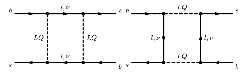
Figure 1: Box diagram for $B_{s}-\bar{B}_{s}$ mixing phenomenon in the leptoquark model.

The mixing amplitude receives additional contribution due to the flow of leptoquark and charged lepton/neutrino in the box diagram as shown in Fig.1. For $X(3,2,7/6)$ LQ, there will be contribution coming only from charged lepton in the loop whereas for $X(3,2,1/6)$ both charged lepton and neutrino will contribute to the mixing amplitude.

The effective Hamiltonian due to the leptoquark $X(3,2,7/6)$ and charged lepton in the loop is given by

$${\cal H}_{eff}=\sum_{i=e,\mu,\tau}\frac{(\lambda^{bi}{\lambda^{si}}^{*})^{2}}{128\pi^{2}}\frac{1}{M_{S}^{2}}~{}I\left(\frac{m_{i}^{2}}{M_{S}^{2}}\right)(\bar{b}\gamma^{\mu}P_{L}s)(\bar{b}\gamma_{\mu}P_{L}s)\;,$$ (20)

where the loop function $I(x)$ is given as

$$I(x)=\frac{1-x^{2}+2x\log x}{(1-x)^{2}},$$ (21)

which is always very close to $I(0)=1$. For $X(3,2,1/6)$ contribution there will be charged lepton as well as neutrinos in the loop and the corresponding effective Hamiltonian becomes

$${\cal H}_{eff}=\sum_{i=e,\mu,\tau}\frac{({\lambda^{bi}}^{*}\lambda^{si})^{2}}{128\pi^{2}}\left[\frac{1}{M_{S}^{2}}~{}I\left(\frac{m_{i}^{2}}{M_{S}^{2}}\right)+\frac{1}{M_{S}^{2}}\right](\bar{b}\gamma^{\mu}P_{R}s)(\bar{b}\gamma_{\mu}P_{R}s)\;.$$ (22)

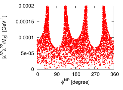
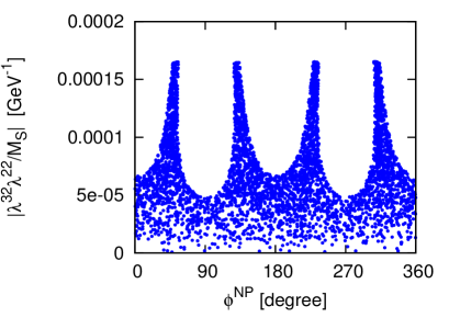
Figure 2: The allowed parameter space for the leptoquark couplings in the $|\lambda^{32}\lambda^{22}/M_{S}|$ vs. $\phi^{NP}$ plane obtained from the mass difference between $B_{s}$ meson mass eigenstates ($\Delta M_{s}$). The left panel corresponds to bounds on $X(3,2,7/6)$ and right panel is for $X(3,2,1/6)$ couplings.

To obtain the constraints on the leptoquark coupling, we require that individual leptoquark contribution to the mass difference does not exceed the $1\sigma$ range of the experimental value. Since we are interested to obtain the bounds on $\lambda^{b\mu}$ and $\lambda^{s\mu}$ couplings, we consider the muon contribution to the mixing amplitude. Neglecting the mass of muon and using Eq. (16), we obtain the contribution due to leptoquark exchange as

$$M_{12}^{LQ} = \frac{{(\lambda^{32}}^{*}{\lambda^{22}})^{2}}{192\pi^{2}M_{S}^{2}}\eta_{B}\hat{B}_{B_{s}}f_{B_{s}}^{2}M_{B_{s}}\;,~{}~{}~{}~{}~{}~{}{\rm for}~{}X(3,2,1/6)$$

$$M_{12}^{LQ} = \frac{(\lambda^{32}{\lambda^{22}}^{*})^{2}}{384\pi^{2}M_{S}^{2}}\eta_{B}\hat{B}_{B_{s}}f_{B_{s}}^{2}M_{B_{s}}\;,~{}~{}~{}~{}~{}~{}{\rm for}~{}X(3,2,7/6).$$ (23)

Thus, including both SM and leptoquark couplings the total contribution to mass difference is given as

$$\Delta M_{s}=\Delta M_{s}^{SM}\left|\left[1+\frac{c}{16G_{F}^{2}V_{tb}^{2}V_{ts}^{*2}m_{W}^{2}S_{0}(x_{t})}\left(\frac{(\lambda^{32}{\lambda^{22}}^{*})^{2}}{M_{S}^{2}}\right)\right]\right|\;,$$ (24)

where the constant $c=1$ for $X(3,2,1/6)$ and $1/2$ for $X(3,2,7/6)$. Now varying the ratio of mass difference $(\Delta M_{s}/\Delta M_{s}^{SM})$ within its $1\sigma$ allowed range (19), we obtain the constraint on $|\lambda^{32}\lambda^{22}/M_{S}|$ as shown in Fig. 2, where the left plot corresponds to constraint on $X(3,2,7/6)$ and the right plot shows the constraint on $X(3,2,1/6)$ couplings. From the figure, the bounds on $|\lambda^{32}\lambda^{22}/M_{S}|$ for the entire allowed range of $\phi^{NP}$ are found to be

$$0\leq\left|\frac{\lambda^{32}\lambda^{22}}{M_{S}}\right|\leq 7.5\times 10^{-5}~{}{\rm GeV}^{-1}\;,~{}~{}~{}~{}~{}~{}~{}~{}{\rm for}~{}X(3,2,7/6),$$

$$0\leq\left|\frac{\lambda^{32}\lambda^{22}}{M_{S}}\right|\leq 5.0\times 10^{-5}~{}{\rm GeV}^{-1}\;,~{}~{}~{}~{}~{}~{}~{}~{}~{}{\rm for}~{}X(3,2,1/6).$$ (25)

It should be noted that using the $B_{s}-\bar{B}_{s}$ mass difference, we obtained the bounds on $|\lambda^{32}\lambda^{22}|/M_{S}$, whereas using the $B_{s}\to\mu\mu$ and $B_{d}\to X_{s}\mu\mu$ data the bounds on $|\lambda^{32}\lambda^{22}|/M_{S}^{2}$ have been obtained. So to correlate these two results, we need to know the mass of the scalar leptoquark $M_{S}$. Recently CMS collaboration cms-lq1 with 8 TeV data set excluded the first generation leptoquarks with masses less than 1010 (850) GeV for $\beta=1.0~{}(0.5)$, where $\beta$ is the branching fraction of a leptoquark decaying to a charged lepton and a quark. The second generation scalar LQs are excluded with masses less than 1080 (760) GeV for $\beta=1.0~{}(0.5)$. They also ruled out at $95\%$ confidence level the single production of first generation LQs with coupling and branching fraction of 1.0 for masses below 1730 GeV and for second generation for masses below 530 GeV cms-lq2 . ATLAS Collaboration excluded at $95\%$ C.L. the scalar leptoquarks with masses upto 1050 GeV for first generation LQs (i.e., $m_{LQ1}<1050$ GeV), $m_{LQ2}<1000$ GeV for second generation LQs and $m_{LQ3}<625$ GeV for third generation LQs atlas-lq . Hence, if we scale the couplings obtained from $B_{s}-\bar{B}_{s}$ mass difference for a benchmark leptoquark mass of 1 TeV, the bounds in Eq. (25) can be translated as

$$0\leq\left|\frac{\lambda^{32}\lambda^{22}}{M_{S}^{2}}\right|\leq 7.5\times 10^{-8}~{}{\rm GeV}^{-2},~{}~{}~{}~{}~{}~{}~{}~{}{\rm for}~{}X(3,2,7/6)$$

$$0\leq\left|\frac{\lambda^{32}\lambda^{22}}{M_{S}^{2}}\right|\leq 5.0\times 10^{-8}~{}{\rm GeV}^{-2},~{}~{}~{}~{}~{}~{}~{}~{}{\rm for}~{}X(3,2,1/6).$$ (26)

Since these bounds are reasonably higher than those of obtained from $B_{s}\to\mu\mu$ and $B_{d}\to X_{s}\mu\mu$ , we will use the bounds (12) as mentioned in the previous section, in our analysis.

IV Analysis of $B_{d}^{0}\rightarrow K^{*}l^{+}l^{-}$ processes

Here we will consider the decay modes $B_{d}^{0}\to K^{*}l^{+}l^{-}$. At the quark level, these processes proceed through the FCNC transition $b\to sl^{+}l^{-}$, which occurs only through loops in the SM, and hence they are quite suitable to look for new physics. Moreover, the dileptons present in these processes allow one to formulate several useful observables which can serve as a testing ground to decipher the presence of new physics.

The transition amplitude for these processes can be obtained using the effective Hamiltonian presented in Eq. (1). The matrix elements of the various hadronic currents between the initial $B$ meson and the final $K^{*}$ vector meson can be parameterized in terms of seven form factors by means of a narrow width approximation. The relevant form factors ball2 are given as

$$\langle K^{*}\left(p_{K^{*}}\right)|\bar{s}\gamma_{\mu}P_{L,R}b|B\left(p\right)\rangle=i\epsilon_{\mu\nu\alpha\beta}\epsilon^{\nu*}p^{\alpha}q^{\beta}\frac{V(s)}{m_{B}+m_{K^{*}}}\mp\frac{1}{2}\Bigg{(}\epsilon^{*}_{\mu}(m_{B}+m_{K^{*}})A_{1}(s)$$

$$-(\epsilon^{*}\cdotp q)(2p-q)_{\mu}\frac{A_{2}(s)}{m_{B}+m_{K^{*}}}-\frac{2m_{K^{*}}}{s}(\epsilon^{*}\cdotp q)\left[A_{3}(s)-A_{0}(s)\right]q_{\mu}\Bigg{)},$$

$$\langle K^{*}\left(p_{K^{*}}\right)|\bar{s}i\sigma_{\mu\nu}q^{\nu}P_{L,R}b|B\left(p\right)\rangle=-i\epsilon_{\mu\nu\alpha\beta}\epsilon^{\nu*}p^{\alpha}q^{\beta}\emph{T}_{1}(s)\pm\frac{1}{2}\Bigg{(}\Big{[}\epsilon^{*}_{\mu}(m^{2}_{B}-m^{2}_{K^{*}})$$

$$-(\epsilon^{*}\cdotp q)(2p-q)_{\mu}\Big{]}\emph{T}_{2}(s)+(\epsilon^{*}\cdotp q)\Bigg{[}q_{\mu}-\frac{s}{(m^{2}_{B}-m^{2}_{K^{*}})}(2p-q)_{\mu}\Bigg{]}\emph{T}_{3}(s)\Bigg{)},$$ (27)

where $q=p_{l^{+}}+p_{l^{-}}$, $s=q^{2}$ and $\epsilon^{\mu}$ is the polarization vector of $K^{*}$. The form factors $A_{1}$, $A_{2}$ and $A_{3}$ are related to each other through

$$A_{3}(s)=\frac{(m_{B}+m_{K^{*}})}{2m_{K^{*}}}A_{1}(s)-\frac{(m_{B}-m_{K^{*}})}{2m_{K^{*}}}A_{2}(s).$$ (28)

The amplitude for the process $B\to K^{*}(\to K\pi)l^{+}l^{-}$ can be represented by seven transversity amplitudes, $A_{\perp,\parallel,0}^{L,R}$ and $A_{t}$. The explicit form of these amplitudes (up to corrections $O(\alpha_{s})$ are presented in Appendix A (B) for low $q^{2}$ (high $q^{2}$) region.

Assuming the $\bar{K}^{*0}\rightarrow K^{-}\pi^{+}$ to be on the mass shell, the full angular distribution of the decay $\bar{B}\rightarrow\bar{K}^{*0}\left(\rightarrow K^{-}\pi^{+}\right)l^{+}l^{-}$ can be described by four independent kinematic variables, the lepton-pair invariant mass and the three angles $\theta_{K^{*}},\theta_{l}$ and $\phi$. The differential decay distribution in terms of three variables can be written as hiller2 ; egede ; egede2

$$\frac{d^{4}\Gamma}{dq^{2}~{}d\cos\theta_{l}~{}d\cos\theta_{K^{*}}~{}d\phi}=\frac{9}{32\pi}J\left(q^{2},\theta_{l},\theta_{K^{*}},\phi\right)\;,$$ (29)

where the lepton spins have been summed over. Here $q^{2}$ is the dilepton invariant mass squared, $\theta_{l}$ is defined as the angle between the negatively charged lepton and the $\bar{B}$ in the dilepton frame, $\theta_{K^{*}}$ is the angle between $K^{-}$ and $\bar{B}$ in the $K^{-}\pi^{+}$ center of mass system and $\phi$ is given by the angle between the normals of the $K^{-}\pi^{+}$ and the dilepton $(l^{+}l^{-})$ planes. The full kinematically physical region phase space is given by

$$4m^{2}_{l}\leqslant q^{2}\leqslant\left(m_{B}-m_{K^{*}}\right)^{2},\hskip 17.07182pt-1\leqslant\cos\theta_{l}\leqslant 1,\hskip 17.07182pt-1\leqslant\cos\theta_{K^{*}}\leqslant 1,\hskip 19.91684pt0\leqslant\phi\leqslant 2\pi.$$ (30)

where $m_{B}$, $m_{K^{*}}$, $m_{l}$ are the masses of $B$ meson, $K^{*}$ and lepton respectively. More explicitly the dependence of the decay distribution on the three angles can be written as

$$J\left(q^{2},\theta_{l},\theta_{K^{*}},\phi\right) = J^{s}_{1}\sin^{2}\theta_{K^{*}}+J^{c}_{1}\cos^{2}\theta_{K^{*}}+\left(J^{s}_{2}\sin^{2}\theta_{K^{*}}+J^{c}_{2}\cos^{2}\theta_{K^{*}}\right)\cos 2\theta_{l}$$ (31)

$$+ J_{3}\sin^{2}\theta_{K^{*}}\sin^{2}\theta_{l}\cos 2\phi+J_{4}\sin 2\theta_{K^{*}}\sin 2\theta_{l}\cos\phi+J_{5}\sin 2\theta_{K^{*}}\sin\theta_{l}\cos\phi$$

$$+ (J_{6}^{s}\sin^{2}\theta_{K^{*}}+J_{6}^{c}\cos^{2}\theta_{K^{*}})\cos\theta_{l}+J_{7}\sin 2\theta_{K^{*}}\sin\theta_{l}\sin\phi$$

$$+ J_{8}\sin 2\theta_{K^{*}}\sin 2\theta_{l}\sin\phi+J_{9}\sin^{2}\theta_{K^{*}}\sin^{2}\theta_{l}\sin 2\phi\;,$$

where the coefficients $J_{i}^{(a)}=J_{i}^{(a)}\left(q^{2}\right)$ for $i=1,....,9$ and $a=s,c$ are functions of the dilepton mass, and are expressed in terms of the transversity amplitudes $A_{0}$, $A_{\parallel}$, $A_{\perp}$, and $A_{t}$ as given in Appendix C.

The dilepton invariant mass spectrum for $\bar{B}\rightarrow\bar{K}^{*}l^{+}l^{-}$ decay after integration over all angles hiller2 is given by

$$\frac{d\Gamma}{dq^{2}}=\frac{3}{4}\left(J_{1}-\frac{J_{2}}{3}\right).$$ (32)

where $J_{i}=2J_{i}^{s}+J_{i}^{c}$. An interesting observable to look for new physics is the zero crossing of forward-backward asymmetry $A_{FB}$, which can be obtained after integrating the 4-differential distribution over $\phi$ and $\theta_{K^{*}}$ angles and is defined as hiller2

$$A_{FB}\left(q^{2}\right) = \left[\int_{-1}^{0}d\cos\theta_{l}\frac{d^{2}\Gamma}{dq^{2}d\cos\theta_{l}}-\int_{0}^{1}d\cos\theta_{l}\frac{d^{2}\Gamma}{dq^{2}d\cos\theta_{l}}\right]\Big{/}\frac{d\Gamma}{dq^{2}}$$ (33)

$$= -\frac{3}{8}\frac{J_{6}}{d\Gamma/dq^{2}}\;.$$

The longitudinal and transverse polarization fraction of the $K^{*}$ meson can be defined in terms of the transversity amplitudes as

$$F_{L}(s)=\frac{|A_{0}|^{2}}{|A_{0}|^{2}+|A_{\parallel}|^{2}+|A_{\perp}|^{2}}\;,~{}~{}~{}~{}~{}~{}~{}F_{T}(s)=\frac{|A_{\parallel}|^{2}+|A_{\perp}|^{2}}{|A_{0}|^{2}+|A_{\parallel}|^{2}+|A_{\perp}|^{2}}\;,$$ (34)

and in terms of the angular coefficients $J_{i}$’s these observables can be expressed as dyk

$$F_{L}\left(s\right)=\frac{3J_{1}^{c}-J_{2}^{c}}{4d\Gamma/dq^{2}}\;,\hskip 42.67912ptF_{T}\left(s\right)=1-F_{L}(s)\,,$$ (35)

so that one can define the ratio of $K^{*}$ polarization fraction $\alpha_{K^{*}}$ as matias2

$$\alpha_{K^{*}}\left(s\right)=\frac{2F_{L}}{F_{T}}-1=\frac{-J_{2}}{2J_{2}^{s}}\;.\hskip 113.81102pt$$ (36)

The transverse asymmetries are given as matias2

$$A_{T}^{(1)}(s) = \frac{-2{\rm Re}\left(A_{\parallel}A^{*}_{\perp}\right)}{|A_{\perp}|^{2}+|A_{\parallel}|^{2}},$$

$$A_{T}^{(2)}\left(s\right) = \frac{J_{3}}{2J^{s}_{2}},$$

$$A_{T}^{(3)}\left(s\right) = \left(\frac{4\left(J_{4}\right)^{2}+\beta^{2}_{l}\left(J_{7}\right)^{2}}{-2J^{c}_{2}\left(2J^{s}_{2}+J_{3}\right)}\right)^{1/2},$$

$$A_{T}^{(4)}\left(s\right) = \left(\frac{4\left(J_{8}\right)^{2}+\beta^{2}_{l}\left(J_{5}\right)^{2}}{4\left(J_{4}\right)^{2}+\beta^{2}_{l}\left(J_{7}\right)^{2}}\right)^{1/2},$$

$$A_{T}^{(5)}\left(s\right) = \frac{|A^{L}_{\perp}A_{\parallel}^{R*}+A^{L}_{\parallel}A_{\perp}^{R*}|}{|A_{\perp}|^{2}+|A_{\parallel}|^{2}},$$

$$A_{\rm Im}\left(s\right) = \frac{J_{9}}{d\Gamma/dq^{2}}.$$ (37)

Another set of interesting observables are the six form factor independent (FFI) observables matias4 , which are given by

$$P_{1}\left(s\right) = \frac{J_{3}}{2J_{2}^{s}}\;,\hskip 42.67912ptP_{2}\left(s\right)=\beta_{l}\frac{J^{s}_{6}}{8J_{2}^{s}}\;,\hskip 42.67912ptP_{3}\left(s\right)=-\frac{J_{9}}{4J_{2}^{s}}\;,$$

$$P_{4}\left(s\right) = \frac{\sqrt{2}J_{4}}{\sqrt{-J_{2}^{c}\left(2J_{2}^{s}-J_{3}\right)}}\;,\hskip 28.45274ptP_{5}\left(s\right)=\frac{\beta_{l}J_{5}}{\sqrt{-2J_{2}^{c}\left(2J_{2}^{s}+J_{3}\right)}}\;,$$

$$P_{6}\left(s\right) = -\frac{\beta_{l}J_{7}}{\sqrt{-2J_{2}^{c}\left(2J_{2}^{s}-J_{3}\right)}}\;.$$ (38)

A slightly modified set of clean observables $P_{4,5,6}^{\prime}$ which are related to $P_{4,5,6}$ through the relations matias

$$P_{4}^{\prime}\equiv P_{4}\sqrt{1-P_{1}}=\frac{J_{4}}{\sqrt{-J_{2}^{c}J_{2}^{s}}}\;,$$

$$P_{5}^{\prime}\equiv P_{5}\sqrt{1+P_{1}}=\frac{J_{5}}{2\sqrt{-J_{2}^{c}J_{2}^{s}}}\;,$$

$$P_{6}^{\prime}\equiv P_{6}\sqrt{1-P_{1}}=\frac{-J_{7}}{2\sqrt{-J_{2}^{c}J_{2}^{s}}}\;.$$ (39)

IV.1 Observables in the large recoil

After getting familiar with the different observables, we now proceed to study these observables in the large recoil limit. For that we need to know the associated form factors for $B\to K^{*}l^{+}l^{-}$ process. In the heavy quark limit the QCDf form factors obey symmetry relations and at leading order in the $1/E$ expansion, they can be expressed in terms of two universal soft non-perturbative form factors $\xi_{\perp}$ and $\xi_{\parallel}$. In order to calculate the universal form factors we use the QCDf scheme hiller2 ; feldmann2 , where they are expressed as

$$\xi_{\perp}(E_{K^{*}})=\frac{m_{B}}{m_{B}+m_{K^{*}}}V(q^{2})\;,\hskip 14.22636pt\xi_{\parallel}(E_{K^{*}})=\frac{m_{B}+m_{K^{*}}}{2E_{K^{*}}}A_{1}(q^{2})-\frac{m_{B}-m_{K^{*}}}{m_{B}}A_{2}(q^{2})\;.$$ (40)

The $q^{2}$ dependence of the form factors $V,~{}A_{1},~{}A_{2}$ can be parameterized as

$$V\left(q^{2}\right)) = \frac{r_{1}}{1-q^{2}/m^{2}_{R}}+\frac{r_{2}}{1-q^{2}/m^{2}_{fit}}\;,$$

$$A_{1}\left(q^{2}\right) = \frac{r_{2}}{1-q^{2}/m^{2}_{fit}}\;,$$

$$A_{2}\left(q^{2}\right) = \frac{r_{1}}{1-q^{2}/m^{2}_{fit}}+\frac{r_{2}}{\left(1-q^{2}/m^{2}_{fit}\right)^{2}}\;.$$ (41)

The values of the parameters involved in the calculation of form factors are taken from ball3 . The $T_{i}$ formfactors are related to the universal form factors $\xi_{\perp,\parallel}$ as

$$T_{1}(q^{2})=\xi_{\perp}(E_{K^{*}})\;,~{}~{}~{}~{}T_{2}(q^{2})=\frac{2E_{K^{*}}}{m_{B}}\xi_{\perp}(E_{K^{*}})\;,~{}~{}~{}~{}T_{3}(q^{2})=\xi_{\perp}(E_{K^{*}})-\xi_{\parallel}(E_{K^{*}})\;.$$ (42)

Table 2: Summary of the values of various input parameters.

	$\alpha$	1/137	$a_{1,\perp}$	0.10
	$\alpha_{s}(M_{z})$	0.1184	$a_{2,\perp}$	0.13
	$m_{b,ps}$	4.6 GeV	$a_{1,\parallel}$	0.10
	$m_{c,pole}$	1.4 GeV	$a_{2,\parallel}$	0.09
	$f_{{K^{*}},\perp}$	0.185 GeV	$\lambda$	0.22537$\pm$0.0006
	$f_{{K^{*}},\parallel}$	0.220 GeV	$A$	$0.814^{+0.023}_{-0.024}$
	$f_{B}$	0.2 GeV	$\bar{\rho}$	0.117 $\pm$ 0.021
			$\bar{\eta}$	0.353 $\pm$ 0.013

After getting familiar with the different observables and the associated form factors for $B\to K^{*}l^{+}l^{-}$ processes in the high recoil limit, we now proceed for numerical estimation. The masses of particles and the lifetime of $B$ meson are taken from pdg . For the leptoquark couplings we use a representative value for the parameter $r$ as $r=0.3$ and vary the associated phase between $\pi/2\leq\phi^{NP}\leq 3\pi/2$. Furthermore, we will present most of the the results only for $X(3,2,7/6)$ LQ and only a few representative plots for $X(3,2,1/6)$. The values of quark masses and all the input parameters used in our analysis are listed in Table-II.

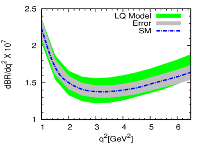
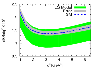
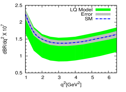
Figure 3: The variation of branching ratios of $\bar{B}\rightarrow\bar{K}^{*}\mu^{+}\mu^{-}$ (left panel) and $\bar{B}\rightarrow\bar{K}^{*}e^{+}e^{-}$ (right panel) with low $q^{2}$ in the standard model and in leptoquark mode. The green bands are due to the leptoquark contributions and the gray bands represent the theoretical uncertainties from the input parameters in the SM. The plots in the top panel are for $X(3,2,7/6)$ and those in the bottom panel are for $X(3,2,1/6)$.

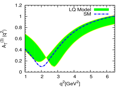
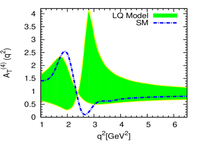
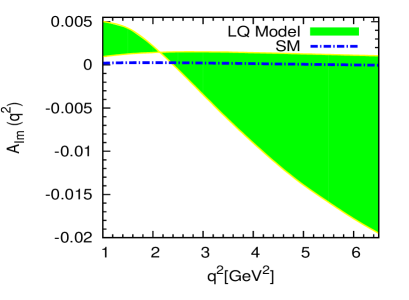
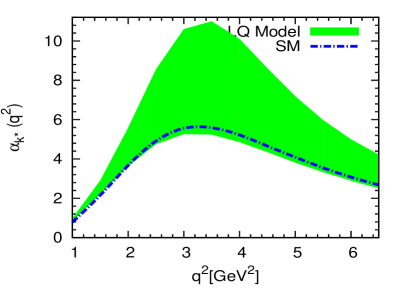
Figure 6: The variation of transverse asymmetry parameters $A_{T}^{(3)}$, $A_{T}^{(4)}$, $A_{\rm Im}$ and the $K^{*}$ polarization factor with $q^{2}$ in high recoil for $X(3,2,7/6)$ LQ.

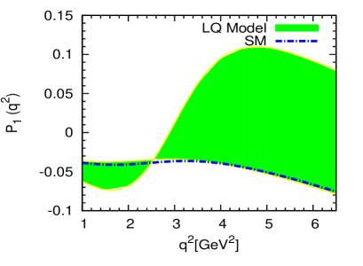
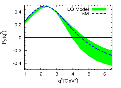
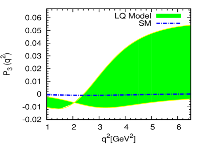
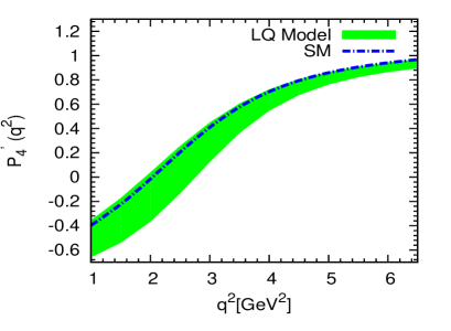
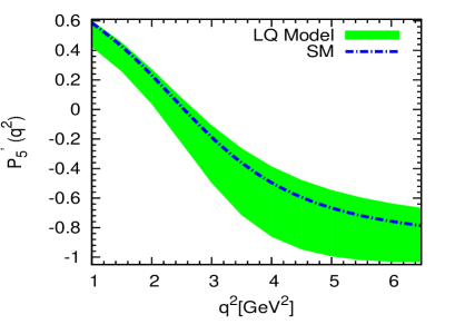
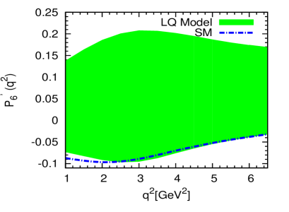
Figure 7: The variation of the observables $P_{1,2,3}$ and $P_{4,5,6}^{\prime}$ with $q^{2}$ for $X(3,2,7/6)$ LQ.

In Fig. 3, we show the variation of the branching ratios for $\bar{B}\rightarrow\bar{K}^{*}\mu^{+}\mu^{-}$ (left panel) and $\bar{B}\rightarrow\bar{K}^{*}e^{+}e^{-}$ (right panel) in the low $q^{2}$ region. The plots in the top panel are for $X(3,2,7/6)$ and those in the bottom panel are for $X(3,2,1/6)$. The variation of the longitudinal and transverse polarization fractions of $K^{*}$ has been shown in Fig. 4 and that of forward-backward asymmetry in Fig. 5. From these figures one can see that the affect of the LQs $X(3,2,7/6)$ and $X(3,2,1/6)$ are quite different and one can easily differentiate between these two models from the measured values of the $K^{*}$ polarization fractions $F_{L}(q^{2})$ and $F_{T}(q^{2})$. The transverse asymmetry parameters $A_{T}^{(3)}$, $A_{T}^{(4)}$, $A_{\rm Im}$ and $K^{*}$ polarization factor $\alpha_{K^{*}}$ variations with $q^{2}$ are presented in Fig. 6. The variation of form factor independent observables as a function of dimuon invariant mass squared have shown in Fig. 7. The total branching ratios and the asymmetries integrated over the range $q^{2}\in[1,6]~{}{\rm GeV^{2}}$ are presented in Table III and the allowed range of transverse asymmetry and the form factor independent observables are given in Table IV. It should be noted that in the leptoquark model these observables deviate significantly from their SM predictions.

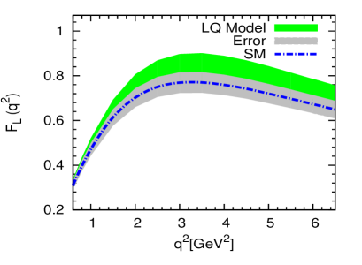
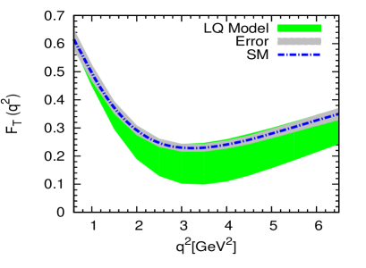
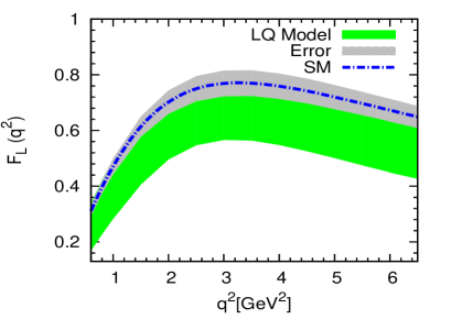
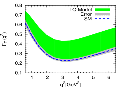
Figure 4: Variation of longitudinal and transverse $K^{*}$ polarization fractions in the low $q^{2}$ region. The plots in the top panel are for $X(3,2,7/6)$ and those in the bottom panel are for $X(3,2,1/6)$.

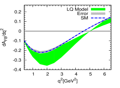
Figure 5: The variation of forward backward asymmetry for $X(3,2,7/6)$ (left panel) and for $X(3,2,1/6)$ (right panel) with $q^{2}$.

Table 3: The predicted values for the integrated branching ratio, forward-backward asymmetry, isospin asymmetry and the polarisation fractions in the range $q^{2}\in[1,6]~{}{\rm GeV}^{2}$ for the $B\to K^{*}\mu^{+}\mu^{-}$ process.

Observables	SM prediction	Values in LQ model	Values in LQ model
		$X(3,2,7/6)$	$X(3,2,1/6)$
BR($B\to K^{*}\mu^{+}\mu^{-}$)	$(7.738\pm 0.464)\times 10^{-7}$	$(6.88\to 8.73)\times 10^{-7}$	$(4.8\to 8.3)\times 10^{-7}$
BR($B\to K^{*}e^{+}e^{-}$)	$(7.742\pm 0.465)\times 10^{-7}$	$(7.03\to 8.73)\times 10^{-7}$	$(4.85\to 8.38)\times 10^{-7}$
$\langle A_{FB}\rangle$	$-(0.09\pm 0.005)$	$-0.11\to 0.004$	$-0.185\to-0.08$
$\langle A_{I}\rangle$	$-(0.03\pm 0.002)$	$-0.06\to-0.04$	$-0.02\to-0.01$
$\langle F_{L}\rangle$	0.71 $\pm$ 0.043	$0.7\to 0.8$	$0.5\to 0.7$
$\langle F_{T}\rangle$	0.29 $\pm$ 0.017	$0.2\to 0.3$	$0.3\to 0.5$

Another interesting observable is the Isospin asymmetry distribution, which has been recently measured by LHCb experiment at 3 fb^-1 data set isospinlhcb . This asymmetry arises due to the non-factorizable part where photon is radiated from the spectator quark in annihilation and spectator scattering. The CP-averaged isospin asymmetry is defined as matias3 ; lord

$$\frac{dA_{I}}{dq^{2}}=\frac{d\Gamma\left[B^{0}\rightarrow K^{*0}l^{+}l^{-}\right]/dq^{2}-d\Gamma\left[B^{\pm}\rightarrow K^{*\pm}l^{+}l^{-}\right]/dq^{2}}{d\Gamma\left[B^{0}\rightarrow K^{*0}l^{+}l^{-}\right]/dq^{2}+d\Gamma\left[B^{\pm}\rightarrow K^{*\pm}l^{+}l^{-}\right]/dq^{2}}\;.$$ (43)

Including longitudinal photon polarizations appearing for $q^{2}\neq 0$, the isospin asymmetry distribution in the QCD factorization scheme is given by

$$A_{I}\left(q^{2}\right)=Re\left(b^{\perp}_{d}\left(q^{2}\right)-b^{\perp}_{u}\left(q^{2}\right)\right)\frac{|C_{9}^{(0)\perp}\left(q^{2}\right)|^{2}}{|C_{10}\left(\mu_{b}\right)|^{2}+|C_{9}^{(0)\perp}\left(q^{2}\right)|^{2}}\times\frac{F\left(q^{2}\right)}{G\left(q^{2}\right)}$$ (44)

with

$$F\left(q^{2}\right)=1+\frac{1}{4}\frac{E^{2}_{K^{*}}m^{2}_{B}}{q^{2}m^{2}_{K^{*}}}\frac{\xi^{2}_{\parallel}\left(q^{2}\right)}{\xi^{2}_{\perp}\left(q^{2}\right)}\frac{Re\left(b^{\parallel}_{d}\left(q^{2}\right)-b^{\parallel}_{u}\left(q^{2}\right)\right)}{Re\left(b^{\perp}_{d}\left(q^{2}\right)-b^{\perp}_{u}\left(q^{2}\right)\right)}\frac{|C_{9}^{(0)\parallel}\left(q^{2}\right)|^{2}}{|C_{9}^{(0)\perp}\left(q^{2}\right)|^{2}}$$ (45)

and

$$G\left(q^{2}\right)=1+\frac{1}{4}\frac{E^{2}_{K^{*}}m^{2}_{B}}{q^{2}m^{2}_{K^{*}}}\frac{\xi^{2}_{\parallel}\left(q^{2}\right)}{\xi^{2}_{\perp}\left(q^{2}\right)}\frac{|C_{9}^{(0)\parallel}\left(q^{2}\right)|^{2}+|C_{10}\left(\mu_{b}\right)|^{2}}{|C_{9}^{(0)\perp}\left(q^{2}\right)|^{2}+|C_{10}\left(\mu_{b}\right)|^{2}}\;,$$ (46)

where the generalized standard model Wilson coefficients are

$$C_{9}^{(0)\perp}\left(q^{2}\right)=C_{9}\left(\mu_{b}\right)+Y\left(q^{2}\right)+\frac{2m_{b}m_{B}}{q^{2}}C_{7}^{eff}\left(\mu_{b}\right)$$ (47)

and

$$C_{9}^{(0)\parallel}\left(q^{2}\right)=C_{9}\left(\mu_{b}\right)+Y\left(q^{2}\right)+\frac{2m_{b}}{m_{B}}C_{7}^{eff}\left(\mu_{b}\right).\hskip 22.76228pt$$ (48)

The $b^{a}_{q}$, $(a=\perp,\parallel)$ terms appearing in the above equations are given as

$$b_{q}^{\perp}\left(q^{2}\right)=\frac{24\pi^{2}m_{B}f_{B}e_{q}}{q^{2}\xi_{\perp}\left(q^{2}\right)C_{9}^{(0)\perp}\left(q^{2}\right)}\left(\frac{f^{\perp}_{K^{*}}}{m_{b}}K^{\perp}_{1}\left(q^{2}\right)+\frac{f_{K^{*}}m_{K^{*}}}{6\lambda_{B,+}\left(q^{2}\right)m_{B}}\frac{K_{2}^{\perp}\left(q^{2}\right)}{1-q^{2}/m^{2}_{B}}\right),$$ (49)

and

$$b_{q}^{\parallel}\left(q^{2}\right)=\frac{24\pi^{2}f_{B}e_{q}m_{K^{*}}}{m_{B}E_{K^{*}}\xi_{\parallel}\left(q^{2}\right)C_{9}^{(0)\parallel}\left(q^{2}\right)}\left(\frac{f_{K^{*}}}{3\lambda_{B,-}\left(q^{2}\right)}K^{\parallel}_{1}\left(q^{2}\right)\right).\hskip 113.81102pt$$ (50)

where the expressions for the terms $K_{1,2}^{a}$ are presented in Appendix E. The variation of isospin asymmetry distribution with respect to dimuon invariant mass squared has given in right panel of Fig. 8 and Table III contains the allowed range of isospin asymmetries.

Table 4: The predicted integrated values of the FFI observables and the CP violating observables in the range $q^{2}\in[1,6]~{}{\rm GeV}^{2}$ for the $B\to K^{*}\mu^{+}\mu^{-}$ process.

Observables	SM prediction	Values in LQ model	Values in LQ model
		$X(3,2,7/6)$	$X(3,2,1/6)$
$\langle P_{1}\rangle$	$-0.044\pm 0.003$	$-0.037\to-0.046$	$-0.017\to 0.14$
$\langle P_{2}\rangle$	0.203 $\pm$ 0.012	0.08 $\to$ 0.23	0.19 $\to$ 0.21
$\langle P_{3}\rangle$	$-(6.0\pm 0.4)\times 10^{-4}$	$-(9.4\to 1.8)\times 10^{-3}$	$-0.014\to 0.08$
$\langle P_{4}\rangle$	0.395 $\pm$ 0.024	0.294 $\to$ 0.45	0.24 $\to$ 0.52
$\langle P_{5}\rangle$	$-0.204\pm 0.012$	$-0.42\to-0.13$	$-0.39\to-0.13$
$\langle P_{6}\rangle$	$-0.0075\pm 0.0005$	$-0.07\to 0.08$	0.079 $\to$ 0.112
$\langle A_{T}^{(3)}\rangle$	0.55 $\pm$ 0.033	0.56 $\to$ 0.6	0.37 $\to$ 0.6
$\langle A_{T}^{(4)}\rangle$	0.87 $\pm$ 0.05	0.82 $\to$ 0.94	0.99 $\to$ 1.5
$\langle A_{Im}\rangle$	$(1.7\pm 0.1)\times 10^{-4}$	$(2.0\to 5.3)\times 10^{-4}$	-0.023 $\to$ 0.005
$\langle\alpha_{K^{*}}\rangle$	3.73 $\pm$ 0.22	3.6 $\to$ 5.6	1.8 $\to$ 3.6

Table 5: The predicted values for the integrated branching ratio, forward-backward asymmetry and isospin asymmetry in the range $q^{2}\in[14.2,19]~{}{\rm GeV}^{2}$ for the $B\to K^{*}\mu^{+}\mu^{-}$ process.

Observables	SM prediction	Values in LQ model $X(3,2,7/6)$
BR($B\to K^{*}\mu^{+}\mu^{-}$)	$(8.5\pm 0.51)\times 10^{-7}$	$(8.93\to 9.31)\times 10^{-7}$
BR($B\to K^{*}e^{+}e^{-}$)	$(8.52\pm 0.511)\times 10^{-7}$	$(8.92\to 9.32)\times 10^{-7}$
$\langle A_{FB}\rangle$	0.4	0.34 $\to$ 0.38
$\langle A_{I}\rangle$	$-(2.75\pm 0.17)\times 10^{-3}$	$(-3.3\to 2.5)\times 10^{-3}$
$\langle P_{2}\rangle$	$-0.42$	$-0.41\to-0.38$
$\langle A_{T}^{(4)}\rangle$	0.57	0.53 $\to$ 0.58
$\langle F_{L}\rangle$	$0.35$	$0.35$
$\langle F_{T}\rangle$	0.65	0.65 $\to$ 0.66

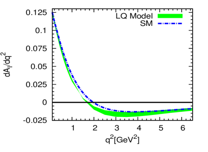
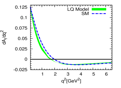
Figure 8: The variation of isospin asymmetry for $X(3,2,7/6)$ (left panel) and for $X(3,2,1/6)$ (right panel) with $q^{2}$.

IV.2 Observables in the low recoil

At low recoil the exclusive $\bar{B}\rightarrow\bar{K}^{*}l^{+}l^{-}$ decays depend on the improved form factor relations and an operator product expansion (OPE) in $1/Q$. The OPE controls the non-perturbative contributions from four-quark operators and is important for charm quark, whose operators enter without any suppression from CKM matrix elements and small Wilson coefficients. The QCD operator identity for massless strange quark $\left(m_{s}=0\right)$ is dyk2 ; dan

$$i\partial^{\nu}\left(\bar{s}i\sigma_{\mu\nu}b\right)=-m_{b}\left(\bar{s}\gamma_{\mu}b\right)+i\partial_{\mu}\left(\bar{s}b\right)-2\left(\bar{s}i\overleftarrow{D}_{\mu}b\right)\;,$$ (51)

which allows to extract relation between the form factors $T_{1}$ and $V$ and the matrix elements of the current $\bar{s}i\overleftarrow{D}_{\mu}b$. The improved Isgur-Wise relations to leading order in $1/m_{b}$ including radiative corrections are

$$T_{1}\left(q^{2}\right) = \kappa V\left(q^{2}\right)\;,$$

$$T_{2}\left(q^{2}\right) = \kappa A_{1}\left(q^{2}\right)\;,$$

$$T_{3}\left(q^{2}\right) = \kappa A_{2}\left(q^{2}\right)\frac{m^{2}_{B}}{q^{2}}\;,$$ (52)

where

$$\kappa=\left(1+\frac{2D_{0}^{(\nu)}\left(\mu\right)}{C_{0}^{\left(\nu\right)}\left(\mu\right)}\right)\frac{m_{b}\left(\mu\right)}{m_{B}}\;.$$ (53)

and at $\mu=m_{b}$ including $\mathcal{O}(\alpha_{s})$ corrections, it reads $\kappa=1+\mathcal{O}(\alpha^{2}_{s})$. We have shown the variation of branching ratio for $\bar{B}\rightarrow\bar{K}^{*}\mu^{+}\mu^{-}$ (left panel) and $\bar{B}\rightarrow\bar{K}^{*}e^{+}e^{-}$ (right panel) with $q^{2}$ in Fig. 9. In the low recoil region the variation of forward-backward asymmetry, isospin asymmetry, longitudinal and transverse polarization fractions of $K^{*}$ with respect to $q^{2}$ are shown in Fig. 10. Fig. 11 shows the variation of $P_{2}$, $A_{T}^{4}$ with respect to dimuon invariant mass squared. Table V contains the integrated values of branching ratio, forward-backward asymmetry and isospin asymmetry in the low recoil i.e. $q^{2}\in[14.2,19]~{}{\rm GeV}^{2}$. It should be noted from these figures that at high $q^{2}$, there is no significant deviation between the SM results and the leptoquark predictions.

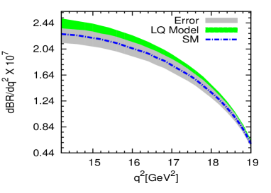
Figure 9: The variation of branching ratio for $\bar{B}\rightarrow\bar{K}^{*}l^{+}l^{-}$ with high $q^{2}$ for $X(3,2,7/6)$ LQ.

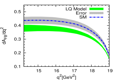
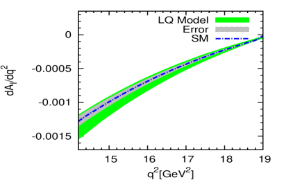
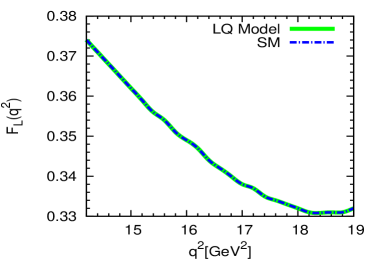
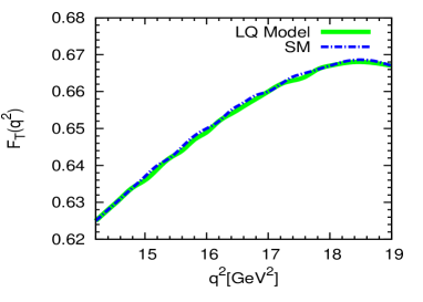
Figure 10: The variation of forward backward asymmetry, isospin asymmetry, longitudinal and transverse polarization fraction with high $q^{2}$ for $X(3,2,7/6)$ LQ.

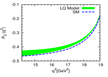
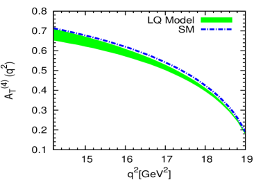
Figure 11: Variation of the observables $P_{2}$, and $A_{T}^{(4)}$ for $X(3,2,7/6)$ LQ.

V Conclusion

In this paper we have studied the rare semileptonic decays $\bar{B}_{d}^{0}\to\bar{K}^{*}l^{+}l^{-}$ using the simple re-normalizable leptoquark model in which a single scalar leptoquark is added to the standard model with the requirement that proton decay would not be induced in perturbation theory. The leptoquark parameter space is constrained using the recent measurement on $B_{s}\rightarrow\mu^{+}\mu^{-}$. Using such parameter space we obtained the bounds on the product of leptoquark couplings. We then estimated the branching ratios, isospin asymmetries and forward-backward asymmetries for $\bar{B}\rightarrow\bar{K}^{*}l^{+}l^{-}$ process in full physical region except the intermediate region of $q^{2}$. The CP violating observables and the form factor independent observables have also been studied in the leptoquark model. It is found that in these models, there could be significant deviations in these observables in high recoil but comparatively less in low recoil regimes. We found that the time-integrated values of some of the asymmetry parameter have deviated significantly from their corresponding SM values, the observation of which in the LHCb experiment would provide the possible existence of leptoquarks.

Acknowledgments

We would like to thank Science and Engineering Research Board (SERB), Government of India for financial support through grant No. SB/S2/HEP-017/2013.

Appendix A Transversity amplitudes at NLO in the large recoil

In the large recoil limit the transversity amplitudes at next to leading order (NLO) within QCDf can be given as hiller2 ; ball

$$A^{L,R}_{\perp} = N\sqrt{2\lambda}\left[\left((C_{9}+C_{9}^{NP}+C_{9}^{\prime NP})\mp(C_{10}+C_{10}^{NP}+C_{10}^{\prime NP}\right)\frac{V\left(q^{2}\right)}{m_{B}+m_{K^{*}}}+\frac{2m_{b}}{q^{2}}\mathcal{T}_{\perp}^{+}\right],$$

$$A_{\parallel}^{L,R} = -N\sqrt{2}\left(m^{2}_{B}-m^{2}_{K^{*}}\right)\Bigg{[}\left((C_{9}+C_{9}^{NP}-C_{9}^{\prime NP})\mp(C_{10}+C_{10}^{NP}-C_{10}^{\prime NP})\right)\frac{A_{1}\left(q^{2}\right)}{m_{B}-m_{K^{*}}}$$

$$\hskip 71.13188pt+\frac{4m_{b}}{m_{B}}\frac{E_{K^{*}}}{q^{2}}\mathcal{T}_{\perp}^{-}\Bigg{]},$$

$$A_{0}^{L,R} = -\frac{N}{2m_{K^{*}}\sqrt{q^{2}}}\Bigg{[}\left((C_{9}+C_{9}^{NP}-C_{9}^{\prime NP})\mp(C_{10}+C_{10}^{NP}-C_{10}^{\prime NP})\right)$$

$$\times \left[\left(m^{2}_{B}-m^{2}_{K^{*}}-q^{2}\right)\left(m_{B}+m_{K^{*}}\right)A_{1}\left(q^{2}\right)-\lambda\frac{A_{2}\left(q^{2}\right)}{m_{B}+m_{K^{*}}}\right]$$

$$+ 2m_{b}\left[\frac{2E_{K^{*}}}{m_{B}}\left(m^{2}_{B}+3m^{2}_{K^{*}}-q^{2}\right)\mathcal{T}_{\perp}^{-}-\frac{\lambda}{m^{2}_{B}-m^{2}_{K^{*}}}\left(\mathcal{T}_{\perp}^{-}+\mathcal{T}_{\parallel}^{-}\right)\right]\Bigg{]}\;,$$

$$A_{t} = \frac{2N}{\sqrt{q^{2}}}\frac{E_{K^{*}}}{m_{K^{*}}}\frac{\xi_{\parallel}}{\Delta_{\parallel}}\sqrt{\lambda}\left(C_{10}+C_{10}^{NP}-C_{10}^{\prime NP}\right)\;,\hskip 56.9055ptA_{S}=0\;,$$ (54)

where $C_{9,10}^{NP}$ and $C_{9,10}^{\prime NP}$ are the new Wilson coefficients arising due to leptoquark exchange and $E_{K}^{*}$ is the energy of the kaon in the $B$ meson rest frame and is given as

$$E_{K^{*}}=\frac{m^{2}_{B}+m^{2}_{K^{*}}-q^{2}}{2m_{B}}\;,$$ (55)

The normalization constant $N$ is given as

$$N=\left[\frac{G^{2}_{F}\alpha^{2}}{3\cdotp 2^{10}\pi^{5}m_{B}}|V_{tb}V^{*}_{ts}|^{2}\hat{s}\sqrt{\lambda}\beta_{l}\right]^{1/2}\;,$$ (56)

where

$$\lambda=m^{4}_{B}+m^{4}_{K^{*}}+q^{4}-2\left(m^{2}_{B}m^{2}_{K^{*}}+m^{2}_{K^{*}}q^{2}+m^{2}_{B}q^{2}\right)\;,~{}~{}~{}~{}~{}{\rm and}~{}~{}~{}~{}~{}\hat{s}=q^{2}/m_{B}^{2}\;.$$ (57)

The transversity amplitude $A_{t}$ contains $\Delta_{\parallel}$ and negligible for massless lepton. It contributes only for $m_{l}\neq 0$. The light-cone distribution amplitude for $K^{*}$ is given by feldmann

$$\Phi_{\bar{K}^{*},a}=6u\left(1-u\right)\{1+a_{1}\left(\bar{K}^{*}\right)_{a}C_{1}^{\left(3/2\right)}\left(2u-1\right)+a_{2}\left(\bar{K}^{*}\right)_{a}C_{2}^{\left(3/2\right)}\left(2u-1\right)\}\;,$$ (58)

where the moments are

$$\lambda^{-1}_{B,+}=\int_{0}^{\infty}d\omega\frac{\Phi_{B,+}\left(\omega\right)}{\omega}\;,\hskip 110.96556pt$$ (59)

$$\lambda^{-1}_{B,-}\left(q^{2}\right)=\frac{e^{-q^{2}/\left(m_{B}\omega_{0}\right)}}{\omega_{0}}\left[-\textbf{E}\textbf{i}\left(q^{2}/m_{B}\omega_{0}\right)+i\pi\right].$$ (60)

The detailed expression for the function $\mathcal{T}_{a}\left(a=\perp,\parallel\right)$ at NLO in the QCDf framework is given in Appendix D.

Appendix B Transversity amplitudes in the low recoil

The transversity amplitudes to leading order in $1/m_{b}$ at low recoil are given as

$$A_{\perp}^{L,R} = i\Bigg{[}\left((C_{9}^{eff}+C_{9}^{NP}+C_{9}^{\prime NP})\mp(C_{10}+C_{10}^{NP}+C_{10}^{\prime NP})\right)+\kappa\frac{2\hat{m}_{b}}{\hat{s}}C_{7}^{eff}\Bigg{]}f_{\perp}\;,$$

$$A_{\parallel}^{L,R} = -i\Bigg{[}\left((C_{9}^{eff}+C_{9}^{NP}-C_{9}^{\prime NP})\mp(C_{10}+C_{10}^{NP}-C_{10}^{\prime NP})\right)+\kappa\frac{2\hat{m}_{b}}{\hat{s}}C_{7}^{eff}\Bigg{]}f_{\parallel}\;,$$

$$A_{0}^{L,R} = -i\Bigg{[}\left((C_{9}^{eff}+C_{9}^{NP}-C_{9}^{\prime NP})\mp(C_{10}+C_{10}^{NP}-C_{10}^{\prime NP})\right)+\kappa\frac{2\hat{m}_{b}}{\hat{s}}C_{7}^{eff}\Bigg{]}f_{0}\;,$$ (61)

where the form factors read

$$f_{\perp}=Nm_{B}\frac{\sqrt{2\hat{\lambda}}}{1+\hat{m}_{K^{*}}}V,\hskip 125.19194pt$$ (62)

$$f_{\parallel}=Nm_{B}\sqrt{2}\left(1+\hat{m}_{K^{*}}\right)A_{1},\hskip 93.89418pt$$ (63)

$$f_{0}=Nm_{B}\frac{\left(1-\hat{s}-\hat{m}^{2}_{K^{*}}\right)\left(1+\hat{m}_{K^{*}}\right)^{2}A_{1}-\hat{\lambda}A_{2}}{2\hat{m}_{K^{*}}\left(1+\hat{m}_{K^{*}}\right)\sqrt{\hat{s}}}\;,$$ (64)

and the normalization factor is

$$N=\left[\frac{G^{2}_{F}\alpha^{2}|\lambda_{t}|^{2}m_{B}\hat{s}\sqrt{\hat{\lambda}}}{3\cdot 2^{10}\pi^{5}}\right]^{1/2}\;.$$ (65)

Here the dimensionless variables are $\hat{s}=q^{2}/m^{2}_{B}$ , $\hat{m}_{i}=m_{i}/m_{B}$ and $\hat{\lambda}=1+\hat{s}^{2}+\hat{m}_{K^{*}}^{4}-2\left(\hat{s}+\hat{s}\hat{m}_{K^{*}}^{2}+\hat{m}_{K^{*}}^{2}\right)$ and the effective coefficients including the four-quark and gluon dipole operators are given by ref43

$$C_{7}^{eff}=C_{7}-\frac{1}{3}\left[C_{3}+\frac{4}{3}C_{4}+20C_{5}+\frac{80}{3}C_{6}\right]+\frac{\alpha_{s}}{4\pi}\left[\left(C_{1}-6C_{2}\right)A(q^{2})-C_{8}F_{8}^{(7)}(q^{2})\right]\;,$$ (66)

$$C_{9}^{eff} = C_{9}+h\left(0,q^{2}\right)\left[\frac{4}{3}C_{1}+C_{2}+\frac{11}{2}C_{3}-\frac{2}{3}C_{4}+52C_{5}-\frac{32}{3}C_{6}\right]$$ (67)

$$- \frac{1}{2}h\left(m_{b},q^{2}\right)\left[7C_{3}+\frac{4}{3}C_{4}+76C_{5}+\frac{64}{3}C_{6}\right]+\frac{4}{3}\left[C_{3}+\frac{16}{3}C_{5}+\frac{16}{9}C_{6}\right]$$

$$+ \frac{\alpha_{s}}{4\pi}\left[C_{1}\left(B(q^{2})+4C(q^{2})\right)-3C_{2}\left(2B\left(q^{2}\right)-C\left(q^{2}\right)\right)-C_{8}F_{8}^{(9)}\left(q^{2}\right)\right]$$

$$+ 8\frac{m^{2}_{c}}{q^{2}}\left[\left(\frac{4}{9}C_{1}+\frac{1}{3}C_{2}\right)(1+\lambda_{u})+2C_{3}+20C_{5}\right]\;.$$

These include the CKM suppressions and the QCD matching corrections at next-to-leading order proportional to $\lambda_{u}=({V_{ub}V^{*}_{us}})/{(V_{tb}V^{*}_{ts})}$, which corresponds to the small amount of CP-violation in the SM.

Appendix C $J_{i}$ coefficients

In terms of the transversity amplitudes $A_{0}$, $A_{\parallel}$, $A_{\perp}$, and $A_{t}$ the $J_{i}$ coefficients can be expressed as ball ; egede

$$J^{s}_{1}=\frac{\left(2+\beta^{2}_{l}\right)}{4}\Bigg{[}|A_{\perp}^{L}|^{2}+|A_{\parallel}^{L}|^{2}+\left(L\rightarrow R\right)\Bigg{]}+\frac{4m^{2}_{l}}{q^{2}}{\rm Re}\left(A_{\perp}^{L}A_{\perp}^{R^{*}}+A_{\parallel}^{L}A_{\parallel}^{R^{*}}\right),$$ (68)

$$J^{c}_{1}=|A_{0}^{L}|^{2}+|A_{0}^{R}|^{2}+\frac{4m^{2}_{l}}{q^{2}}\Bigg{[}|A_{t}|^{2}+2{\rm Re}\left(A_{0}^{L}A_{0}^{R^{*}}\right)\Bigg{]}+\beta^{2}_{l}|A_{S}|^{2},\hskip 59.75095pt$$ (69)

$$J^{s}_{2}=\frac{\beta^{2}_{l}}{4}\left[|A_{\perp}^{L}|^{2}+|A_{\parallel}^{L}|^{2}+\left(L\rightarrow R\right)\right],\hskip 179.25244pt$$ (70)

$$J^{c}_{2}=-\beta^{2}_{l}\left[|A_{0}^{L}|^{2}+\left(L\rightarrow R\right)\right],\hskip 216.2411pt$$ (71)

$$J_{3}=\frac{1}{2}\beta^{2}_{l}\left[|A_{\perp}^{L}|^{2}-|A_{\parallel}^{L}|^{2}+\left(L\rightarrow R\right)\right],\hskip 176.407pt$$ (72)

$$J_{4}=\frac{1}{\sqrt{2}}\beta^{2}_{l}\left[{\rm Re}\left(A_{0}^{L}A_{\parallel}^{L^{*}}\right)+\left(L\rightarrow R\right)\right],\hskip 173.56198pt$$ (73)

$$J_{5}=\sqrt{2}\beta_{l}\left[{\rm Re}\left(A_{0}^{L}A_{\perp}^{L^{*}}\right)-\left(L\rightarrow R\right)-\frac{m_{l}}{\sqrt{q^{2}}}{\rm Re}\left(A_{\parallel}^{L}A^{*}_{S}+A_{\parallel}^{R}A^{*}_{S}\right)\right],\hskip 31.2982pt$$ (74)

$$J^{s}_{6}=2\beta_{l}\left[{\rm Re}\left(A_{\parallel}^{L}A_{\perp}^{L^{*}}\right)-\left(L\rightarrow R\right)\right],\hskip 184.9429pt$$ (75)

$$J^{c}_{6}=4\beta_{l}\frac{m_{l}}{\sqrt{q^{2}}}{\rm Re}\left[A_{0}^{L}A_{S}^{*}+\left(L\rightarrow R\right)\right],\hskip 179.25244pt$$ (76)

$$J_{7}=\sqrt{2}\beta_{l}\left[{\rm Im}\left(A_{0}^{L}A_{\parallel}^{L^{*}}\right)-\left(L\rightarrow R\right)+\frac{m_{l}}{\sqrt{q^{2}}}{\rm Im}\left(A_{\perp}^{L}A^{*}_{S}+A_{\perp}^{R}A^{*}_{S}\right)\right],\hskip 28.45274pt$$ (77)

$$J_{8}=\frac{1}{\sqrt{2}}\beta^{2}_{l}\left[{\rm Im}\left(A_{0}^{L}A_{\perp}^{L^{*}}\right)+\left(L\rightarrow R\right)\right],\hskip 173.56198pt$$ (78)

$$J_{9}=\beta^{2}_{l}\left[{\rm Im}\left(A_{\parallel}^{L^{*}}A_{\perp}^{L}\right)+\left(L\rightarrow R\right)\right],\hskip 190.63338pt$$ (79)

where

$$\beta_{l}=\sqrt{1-\frac{4m^{2}_{l}}{q^{2}}}\;,$$ (80)

and

$$A_{i}A_{j}^{*}=A_{i}^{L}\left(q^{2}\right)A^{*L}_{j}\left(q^{2}\right)+A_{i}^{R}\left(q^{2}\right)A^{*R}_{j}\left(q^{2}\right)\hskip 28.45274pt\left(i,j=0,\parallel,\perp\right),$$ (81)

in shorthand notation. The transversity amplitudes $A_{i}^{L,R}$ are presented in the appendix for A (B) for low (high) $q^{2}$ region.

Appendix D $\mathcal{T}_{a}^{\pm}$ calculation

The $B\rightarrow K^{*}$ matrix elements in large recoil limit depend on four independent functions $\mathcal{T}_{a}^{\pm}$ corresponding to a transversely $\left(a=\perp\right)$ and longitudinally $\left(a=\parallel\right)$ polarized $K^{*}$ and at next-to-leading order is given by feldmann

$$\mathcal{T}_{a}=\xi_{a}C_{a}+\frac{\pi^{2}}{N_{c}}\frac{f_{B}f_{K^{*},a}}{m_{B}}\Xi_{a}\sum\limits_{\pm}\int\frac{d\omega}{\omega}\Phi_{B,\pm}\left(\omega\right)\int_{0}^{1}du\Phi_{K^{*},a}\left(u\right)\mathcal{T}_{a,\pm}\left(u,\omega\right)\;,$$ (82)

where $\Xi_{\perp}\equiv 1$, $\Xi_{\parallel}\equiv m_{K^{*}}/E_{K^{*}}$ and the factorization scale $\mu_{f}=\sqrt{m_{b}\Lambda_{QCD}}$.
The coefficient functions $C_{a}$ and $\mathcal{T}_{a,\pm}$ can be written as

$$C_{a}=C_{a}^{(0)}+\frac{\alpha_{s}\left(\mu_{b}\right)C_{F}}{4\pi}C_{a}^{(1)}\;,\hskip 56.9055pt$$ (83)

and

$$\mathcal{T}_{a,\pm}=\mathcal{T}_{a,\pm}^{(0)}\left(u,\omega\right)+\frac{\alpha_{s}\left(\mu_{f}\right)C_{F}}{4\pi}\mathcal{T}_{a,\pm}^{(1)}\left(u,\omega\right)\;.$$ (84)

The form factor terms $C_{a}^{\left(0\right)}$ at leading order are

$$C_{\perp}^{\left(0\right)}=C_{7}^{eff}+\frac{q^{2}}{2m_{b}m_{B}}Y\left(q^{2}\right)\;,$$ (85)

$$C_{\parallel}^{\left(0\right)}=-C_{7}^{eff}-\frac{m_{B}}{2m_{b}}Y\left(q^{2}\right)\;.$$ (86)

The coefficients $C_{a}^{\left(1\right)}$ at next-to-leading order can be divided into a factorizable and a non-factorizable part as

$$C_{a}^{\left(1\right)}=C_{a}^{\left(f\right)}+C_{a}^{\left(nf\right)}\;.$$ (87)

At NLO the factorizable correction reads

$$C_{\perp}^{\left(f\right)}=C_{7}^{eff}\left(\ln\frac{m_{b}^{2}}{\mu^{2}}-L+\Delta M\right)\;,$$ (88)

$$C_{\parallel}^{\left(f\right)}=-C_{7}^{eff}\left(\ln\frac{m_{b}^{2}}{\mu^{2}}+2L+\Delta M\right)\;,$$ (89)

and the non-factorizable correction for heavy to light transitions are

$$C_{F}C_{\perp}^{\left(nf\right)} = -\bar{C}_{2}F_{2}^{\left(7\right)}-C_{8}^{eff}F_{8}^{\left(7\right)}-\frac{q^{2}}{2m_{b}m_{B}}\left[\bar{C_{2}}F_{2}^{\left(9\right)}+2\bar{C}_{1}\left(F_{1}^{\left(9\right)}+\frac{1}{6}F_{2}^{\left(9\right)}\right)+C_{8}^{eff}F_{8}^{\left(9\right)}\right],$$

$$C_{F}C_{\parallel}^{\left(nf\right)} = \bar{C}_{2}F_{2}^{\left(7\right)}+C_{8}^{eff}F_{8}^{\left(7\right)}+\frac{m_{B}}{2m_{b}}\left[\bar{C_{2}}F_{2}^{\left(9\right)}+2\bar{C}_{1}\left(F_{1}^{\left(9\right)}+\frac{1}{6}F_{2}^{\left(9\right)}\right)+C_{8}^{eff}F_{8}^{\left(9\right)}\right]\;,$$ (90)

where $L$ and $\Delta M$ have given in Ref. feldmann . At leading order the hard-spectator scattering term $\mathcal{T}_{a,\pm}^{(0)}\left(u,\omega\right)$ from weak annihilation diagram is given as

$$\mathcal{T}_{\perp,+}^{(0)}\left(u,\omega\right)=\mathcal{T}_{\perp,-}^{(0)}\left(u,\omega\right)=\mathcal{T}_{\parallel,+}^{(0)}\left(u,\omega\right)=0\;,$$ (91)

$$\hskip 28.45274pt\mathcal{T}_{\parallel,-}^{(0)}\left(u,\omega\right)=-e_{q}\frac{m_{B}\omega}{m_{B}\omega-q^{2}-i\epsilon}\frac{4m_{B}}{m_{b}}\left(\bar{C}_{3}+3\bar{C_{4}}\right)\;.$$ (92)

The hard scattering functions $\mathcal{T}_{a}^{(1)}$ at next to leading order contain a factorisable as well as non-factorizable part

$$\mathcal{T}_{a}^{(1)}=\mathcal{T}_{a}^{(f)}+\mathcal{T}_{a}^{(nf)}\;.$$ (93)

Including $\mathcal{O}\left(\alpha_{s}\right)$ corrections the factorizable term to the hard scattering functions $\mathcal{T}_{a,\pm}^{(1)}$ are given by

$$\mathcal{T}_{\perp,+}^{(f)}\left(u,\omega\right)=C_{7}^{eff}\frac{2m_{B}}{\bar{u}E_{K^{*}}}\;,\hskip 28.45274pt$$ (94)

$$\mathcal{T}_{\perp,-}^{(f)}\left(u,\omega\right)=\mathcal{T}_{\parallel,-}^{(f)}\left(u,\omega\right)=0\;,$$ (95)

$$\mathcal{T}_{\parallel,+}^{(f)}\left(u,\omega\right)=C_{7}^{eff}\frac{4m_{B}}{\bar{u}E_{K^{*}}}\;,\hskip 28.45274pt$$ (96)

and the non-factorizable correction can be computed by solving the matrix elements of four-quark operators and the chromomagnetic dipole operator

$$\mathcal{T}_{\perp,+}^{(nf)}\left(u,\omega\right) = -\frac{4e_{d}C_{8}^{eff}}{u+\bar{u}q^{2}/m_{B}^{2}}+\frac{m_{B}}{2m_{b}}[e_{u}t_{\perp}\left(u,m_{c}\right)\left(\bar{C_{2}}+\bar{C_{4}}-\bar{C_{6}}\right)$$ (97)

$$+ e_{d}t_{\perp}\left(u,m_{b}\right)\left(\bar{C_{3}}+\bar{C_{4}}-\bar{C_{6}}-4m_{b}/m_{B}\bar{C_{5}}\right)+e_{d}t_{\perp}\left(u,0\right)\bar{C_{3}}]\;,$$

$$\mathcal{T}_{\perp,-}^{(nf)}\left(u,\omega\right)=0\;,\hskip 278.83708pt$$ (98)

$$\mathcal{T}_{\parallel,+}^{(nf)}\left(u,\omega\right) = \frac{m_{B}}{m_{b}}[e_{u}t_{\parallel}\left(u,m_{c}\right)\left(\bar{C_{2}}+\bar{C_{4}}-\bar{C_{6}}\right)$$ (99)

$$+ e_{d}t_{\parallel}\left(u,m_{b}\right)\left(\bar{C_{3}}+\bar{C_{4}}-\bar{C_{6}}\right)+e_{d}t_{\parallel}\left(u,0\right)\bar{C_{3}}]\;,$$

$$\mathcal{T}_{\parallel,-}^{(nf)}\left(u,\omega\right) = e_{q}\frac{m_{B}\omega}{m_{B}\omega-q^{2}-i\epsilon}\Bigg{[}\frac{8C_{8}^{eff}}{\bar{u}+uq^{2}/m_{B}^{2}}$$ (100)

$$+ \frac{6m_{B}}{m_{b}}\Bigg{(}h\left(\bar{u}m_{B}^{2}+uq^{2},m_{c}\right)\left(\bar{C}_{2}+\bar{C}_{4}+\bar{C}_{6}\right)$$

$$+ h\left(\bar{u}m_{B}^{2}+uq^{2},m_{b}^{pole}\right)\left(\bar{C}_{3}+\bar{C}_{4}+\bar{C}_{6}\right)$$

$$+ h\left(\bar{u}m_{B}^{2}+uq^{2},0\right)\left(\bar{C}_{3}+3\bar{C}_{4}+3\bar{C}_{6}\right)-\frac{8}{27}\left(\bar{C}_{3}-\bar{C}_{5}-15\bar{C}_{6}\right)\Bigg{)}\Bigg{]}.$$

The $t_{a}\left(u,m_{q}\right)$ functions are given by

$$t_{\perp}\left(u,m_{q}\right) = \frac{2m_{B}}{\bar{u}E_{K^{*}}}I_{1}\left(m_{q}\right)+\frac{q^{2}}{\bar{u}^{2}E^{2}_{K^{*}}}\left(B_{0}\left(\bar{u}m_{B}^{2}+uq^{2},m_{q}\right)-B_{0}\left(q^{2},m_{q}\right)\right),$$

$$t_{\parallel}\left(u,m_{q}\right) = \frac{2m_{B}}{\bar{u}E_{K^{*}}}I_{1}\left(m_{q}\right)+\frac{\bar{u}m_{B}^{2}+uq^{2}}{\bar{u}^{2}E^{2}_{K^{*}}}\left(B_{0}\left(\bar{u}m_{B}^{2}+uq^{2},m_{q}\right)-B_{0}\left(q^{2},m_{q}\right)\right)\;,$$ (101)

where $B_{0}$ and $I_{1}$ are

$$B_{0}\left(q^{2},m_{q}\right)=-2\sqrt{4m^{2}_{q}/q^{2}-1}\arctan\frac{1}{\sqrt{4m^{2}_{q}/q^{2}-1}}\;,\hskip 65.44142pt$$ (102)

$$I_{1}\left(m_{q}\right)=1+\frac{2m^{2}_{q}}{\bar{u}\left(m^{2}_{B}-q^{2}\right)}\left[L_{1}\left(x_{+}\right)+L_{1}\left(x_{-}\right)-L_{1}\left(y_{+}\right)-L_{1}\left(y_{-}\right)\right]\;,$$ (103)

and

$$x_{\pm}=\frac{1}{2}\pm\left(\frac{1}{4}-\frac{m^{2}_{q}}{\bar{u}m_{B}^{2}+uq^{2}}\right)^{1/2},\hskip 22.76228pty_{\pm}=\frac{1}{2}\pm\left(\frac{1}{4}-\frac{m^{2}_{q}}{q^{2}}\right)^{1/2}\;,$$ (104)

$$L_{1}\left(x\right)=\ln\frac{x-1}{x}\ln\left(1-x\right)-\frac{\pi^{2}}{6}+Li_{2}\left(\frac{x}{x-1}\right)\;.\hskip 65.44142pt$$ (105)

Appendix E Functions involved in Isospin asymmetry parameter

The function $K_{1}^{\parallel}$ receives an annihilation contribution to leading order and the function $K_{1,2}^{\perp}$ appear at subleading order of the $\Lambda_{h}/m_{B}$ expansion. The meson photon transition form factors and their role in the annihilation contribution to $B$ meson decays has been given by the function with superscript (a). Here only transverse polarization contributes and there are no contributions from $C_{5}$ and $C_{6}$. The function $K_{1,2}^{(b)}$ contain the decay amplitude from the diagram of hard spectator interactions involving the gluonic penguin operator $\mathcal{O}_{8}$ and the contributions of the hard spectator interactions diagrams involving the operator $\mathcal{O}_{1-6}$ have been included in $K_{1,2}^{(b)}$.
The functions $K^{\parallel}_{1}$ and $K^{\perp}_{1,2}$ defined via $b^{a}_{q}$ is given as lord

$$K_{1}^{\perp}\left(q^{2}\right)=K_{1}^{\perp\left(a\right)}\left(q^{2}\right)+K_{1}^{\perp\left(b\right)}\left(q^{2}\right)+K_{1}^{\perp\left(c\right)}\left(q^{2}\right)\;,\hskip 113.81102pt$$ (106)

with

$$K_{1}^{\perp\left(a\right)}\left(q^{2}\right)=-\left(\bar{C}_{6}\left(\mu_{h}\right)+\frac{\bar{C}_{5}\left(\mu_{h}\right)}{N_{c}}\right)F_{\perp}\left(\hat{s}\right),\hskip 22.76228ptF_{\perp}\left(\hat{s}\right)=\frac{1}{3}\int_{0}^{1}du\frac{\phi_{K^{*}}^{\perp}\left(u\right)}{\bar{u}+u\hat{s}},$$

$$K_{1}^{\perp\left(b\right)}\left(q^{2}\right)=C^{eff}_{8}\left(\mu_{h}\right)\frac{m_{b}}{m_{B}}\frac{C_{F}}{N_{c}}\frac{\alpha_{s}\left(\mu_{h}\right)}{4\pi}X_{\perp}\left(\hat{s}\right),~{}~{}~{}X_{\perp}\left(\hat{s}\right)=F_{\perp}\left(\hat{s}\right)+\frac{1}{3}\int_{0}^{1}du\frac{\phi_{K^{*}}^{\perp}\left(u\right)}{(\bar{u}+u\hat{s})^{2}},$$

$$K_{1}^{\perp\left(c\right)}\left(q^{2}\right)=\frac{C_{F}}{N_{c}}\frac{\alpha_{s}\left(\mu_{h}\right)}{4\pi}\frac{2}{3}\int_{0}^{1}du\frac{\phi_{K^{*}}^{\perp}\left(u\right)}{\bar{u}+u\hat{s}}F_{V}\left(\bar{u}m_{B}^{2}+uq^{2}\right)$$ (107)

and

$$K_{2}^{\perp}\left(q^{2}\right)=K_{2}^{\perp\left(a\right)}\left(q^{2}\right)+K_{2}^{\perp\left(b\right)}\left(q^{2}\right)+K_{2}^{\perp\left(c\right)}\left(q^{2}\right)\;,\hskip 113.81102pt$$ (108)

with

$$K_{2}^{\perp\left(a\right)}\left(q^{2}\right)=-\frac{\lambda_{u}}{\lambda_{t}}\left(\frac{\bar{C}_{1}}{3}\left(\mu_{h}\right)+\bar{C}_{2}\left(\mu_{h}\right)\right)\delta_{qu}+\left(\bar{C}_{4}\left(\mu_{h}\right)+\frac{\bar{C}_{3}\left(\mu_{h}\right)}{3}\right)\;,$$

$$K_{2}^{\perp\left(b\right)}\left(q^{2}\right)=\mathcal{O}\left(\frac{\Lambda_{h}}{m_{B}}\right)\;,$$

$$K_{2}^{\perp\left(c\right)}\left(q^{2}\right)=-\frac{C_{F}}{N_{c}}\frac{\alpha_{s}\left(\mu_{h}\right)}{4\pi}\frac{1}{2}\int_{0}^{1}du\left(g_{\perp}^{(\nu)}\left(u\right)-\frac{g_{\perp}^{{}^{\prime}(a)}\left(u\right)}{4}\right)F_{V}\left(\bar{u}m_{B}^{2}+uq^{2}\right)\;.$$ (109)

For parallel case in Eq. (61),

$$K_{1}^{\parallel}\left(q^{2}\right)=K_{1}^{\parallel\left(a\right)}\left(q^{2}\right)+K_{1}^{\parallel\left(b\right)}\left(q^{2}\right)+K_{1}^{\parallel\left(c\right)}\left(q^{2}\right)\;,\hskip 85.35826pt$$ (110)

with

$$K_{1}^{\parallel\left(a\right)}\left(q^{2}\right)=K_{2}^{\perp\left(a\right)}\left(q^{2}\right),$$

$$K_{1}^{\parallel\left(b\right)}\left(q^{2}\right)=-C^{eff}_{8}\left(\mu_{h}\right)\frac{m_{b}}{m_{B}}\frac{C_{F}}{N_{c}}\frac{\alpha_{s}\left(\mu_{h}\right)}{4\pi}F_{\parallel}\left(\hat{s}\right),\hskip 22.76228ptF_{\parallel}\left(\hat{s}\right)=2\int_{0}^{1}du\frac{\phi_{\parallel}\left(u\right)}{\bar{u}+u\hat{s}},$$

$$K_{1}^{\parallel\left(c\right)}\left(q^{2}\right)=-\frac{C_{F}}{N_{c}}\frac{\alpha_{s}\left(\mu_{h}\right)}{4\pi}2\int_{0}^{1}du\phi_{\parallel}\left(u\right)F_{V}\left(\bar{u}m_{B}^{2}+uq^{2}\right)\;.$$ (111)

The vector form factor $F_{V}\left(s\right)$ is given by

$$F_{V}\left(s\right) = \frac{3}{4}\{h\left(s,m_{c},\mu_{h}\right)\left(\bar{C}_{2}\left(\mu_{h}\right)+\bar{C}_{4}\left(\mu_{h}\right)+\bar{C}_{6}\left(\mu_{h}\right)\right)$$ (112)

$$+ h\left(s,m_{b},\mu_{h}\right)\left(\bar{C}_{3}\left(\mu_{h}\right)+\bar{C}_{4}\left(\mu_{h}\right)+\bar{C}_{6}\left(\mu_{h}\right)\right)$$

$$+ h\left(s,0,\mu_{h}\right)\left(\bar{C}_{3}\left(\mu_{h}\right)+3\bar{C}_{4}\left(\mu_{h}\right)+3\bar{C}_{6}\left(\mu_{h}\right)\right)$$

$$- \frac{8}{27}\left(\bar{C}_{3}\left(\mu_{h}\right)-\bar{C}_{5}\left(\mu_{h}\right)-15\bar{C}_{6}\left(\mu_{h}\right)\right)\}\;.$$

References

- (1) R. Aaij et al., [LHCb Collaboration], Phys. Rev. Lett. 111, 191801 (2013) [arXiv:1308.1707].
- (2) R. Aaij et al., [LHCb Collaboration], JHEP 1406, 133 (2014) [arXiv:1403.8044]. [hep-ex].
- (3) R. Aaij et al., [LHCb Collaboration], JHEP 1307, 084 (2013) [arXiv:1305.2168].
- (4) R. Aaij et al., [LHCb Collaboration], Phys. Rev. Lett. 113, 151601 (2014) [arXiv:1406.6482].
- (5) C. Langenbruch on behalf of the LHCb collaboration, [arXiv: 1505.04160].
- (6) B. Grinstein, D. Pirjol, Phys. Rev. D 70, 114005 (2004) [arXiv:hep-ph/0404250].
- (7) M. Beylich, G. Buchalla and T. Feldmann, Eur. Phys. J. C 71, 1635 (2011) [arXiv:1101.5118 [hep-ph]]; G. Buchalla and G. Isidori, Nucl. Phys.B 525, 333 (1998) [hep-ph/9801456].
- (8) B. Grinstein and D. Pirjol, Phys. Lett. B 533, 8 (2002) [arXiv:hep-ph/0201298].
- (9) S. Descotes-Genon, J. Matias, M. Ramon, J. Virto, JHEP 01, 048 (2013) [arXiv:1207.2753].
- (10) S. Jäger, J. Martin Camalich, JHEP 05, 043 (2013) [arXiv:1212.2263]; S.Descotes-Genon, L. Hofer, J. Matias and J. Virto, JHEP 1412, 125 (2014) [arXiv:1407.8526].
- (11) T. Huber, T. Hurth and E. Lunghi, Nucl. Phys. B 802, 40 (2008), [arXiv:0712.3009].
- (12) F. Beaujean, C. Bobeth, and D. van Dyk, Eur. Phys. J. C 74, 2897, (2014) [arXiv:1310.2478]; T. Hurth and F. Mahmoudi, JHEP 04, 097 (2014) [arXiv:1312.5267]; W. Altmannshofer, S. Gori, M. Pospelov, and I. Yavin, Phys. Rev. D 89, 095033 (2014) [arXiv: 1403.1269]; R. Gauld, F. Goertz, and U. Haisch, JHEP 01, 069 (2014) [arXiv:1310.1082]; R. Gauld, F. Goertz, and U. Haisch, Phys. Rev. D 89, 015005 (2014) [arXiv:1308.1959]; A. Datta, M. Duraisamy, and D. Ghosh, Phys. Rev. D 89, 071501 (2014) [arXiv:1310.1937]; A. J. Buras and J. Girrbach, JHEP 12, 009 (2013) [arXiv:1309.2466]; A. J. Buras, F. De Fazio, and J. Girrbach, JHEP 02, 112 (2014) [arXiv:1311.6729]; S. Descotes-Genon, J. Matias and J. Virto, Phys. Rev. D 88, 074002 (2013)[arXiv:1307.5683 [hep-ph]]; R. R. Horgan, Z. Liu, S. Meinel, and M. Wingate, Phys. Rev. Lett. 112, 212003 (2014) [arXiv: 1310.3887]; A. J. Buras, J. Girrbach-Noe, C. Niehoff, and D. M. Straub, JHEP 02, 184 (2015) [arXiv:1409.4557]; A. Crivellin, arXiv: 1409.0922; D. Ghosh, M. Nardecchia, and S. Renner, JHEP 12, 131 (2014) [arXiv:1408.4097]; G. Hiller and M. Schmaltz, Phys. Rev. D 90, 054014 (2014) [arXiv:1408.1627]; T. Hurth, F.Mahmoudi, and S. Neshatpour, JHEP 12, 053 (2014) [arXiv: 1410.4545]; S. L. Glashow, D. Guadagnoli, K. Lane, Phys. Rev. Lett. 114, 091801 (2015) [arXiv:1411.0565].
- (13) D. Aristizabal sierra, F. Staub and A. Vicente, Phys. Rev. D 92, 015001 (2015) [arXiv:1503.06077 [hep-hp]]; Sofiane M. Boucenna, Jose W.F. Valle and A. Vicente, [arXiv:1503.07099]; F. Mahmoudi, S. Neshatpour, J. Virto, Eur. Phys. J. C74 (2014) 2927, [arXiv:1401.2145]; A. Crivellin, G. D’Ambrasio, J. Heeck, Phys. Rev. Lett. 114, 151801 (2015) [arXiv:1501.00993]; A. Crivellin, G. D’Ambrasio, J. Heeck, Phys. Rev. D 91, 075006 (2015) [arXiv:1503.03477 [hep-hp]]; A. Crivellin, L. Hofer, J. Matias, U. Nierste, S. Pokorski, J. Rosiek, Phys. Rev. D 92, 054013 (2015) [arXiv:1504.07928]; Xian-Wei Kang, B. Kubis, C. Hanhart, Ulf-G. Meibner, Phys Rev. D 89, 053015 (2014), [arXiv:1312.1193]; J. Lyon, R. Zwicky, [arXiv:1406:0566]; J. Gratex, M. Hopfer, R. Zwicky, [arXiv: 1506.03970].
- (14) H. Georgi and S. L. Glashow, Phys. Rev. Lett. 32, 438 (1974); H. Fritzsch and P. Minkowski, Annals Phys. 93, 193 (1975); P. Langacker, Phys. Rep. 72 185 (1981).
- (15) J. C. Pati and A. Salam, Phys. Rev. D 10, 275 (1974).
- (16) D. B. Kaplan, Nucl. Phys. B 365, 259 (1991).
- (17) B. Schrempp and F. Shrempp, Phys. Lett. B 153, 101 (1985); B. Gripaios, JHEP 02, 045 (2010) [arXiv:0910.1789].
- (18) J. M. Arnold, B. Fornal and M. B. Wise, Phys. Rev. D 88, 035009 (2013), [arXiv:1304.6119].
- (19) S. Davidson, D. C. Bailey and B. A. Campbell, Z. Phys. C 61, 613 (1994), hep-ph/9309310; I. Dorsner, S. Fajfer, J. F. Kamenik, N. Kosnik, Phys. Lett. B 682, 67 (2009); [arXiv:0906.5585]; S. Fajfer, N. Kosnik, Phys. Rev. D 79, 017502 (2009), [arXiv:0810.4858]; R. Benbrik, M. Chabab, G. Faisel, arXiv:1009.3886 [hep-ph]; A. V. Povarov, A. D. Smirnov, arXiv:1010.5707 [hep-ph]; J. P Saha, B. Misra and A. Kundu, Phys. Rev.D 81, 095011 (2010), [arXiv:1003.1384]; I. Dorsner, J. Drobnak, S. Fajfer, J. F. Kamenik, N. Kosnik, JHEP 11, 002 (2011), [arXiv: 1107.5393].
- (20) N. Kosnik, Phys. Rev. D 86, 055004 (2012), arXiv:1206.2970 [hep-ph].
- (21) F. S. Queiroz, K. Sinha, A. Strumia, arXiv:1409.6301 [hep-ph]; B. Allanach, A. Alves, F. S. Queiroz, K. Sinha, A. Strumia, arXiv:1501.03494.
- (22) L. Calibbi, A. Crivellin, T. Ota, [arXiv:1506.02661 [hep-hp]]; Ivo de M. Varzielas, G. Hiller, JHEP 1506 (2005) 072, [arXiv:1503.01084]; D. Becirevic, S. Faster, N. Kosnik, Phys Rev. D 92, 014016 (2015) [arXiv:1503.09024].
- (23) A. J. Buras and M. Münz, Phys. Rev. D 52, 186 (1995); M. Misiak, Nucl. Phys. B 393, 23 (1993); ibid. 439, 461 (E) (1995).
- (24) W.-S. Hou, M. Kohda and F. Xu, Phys. Rev. D 90, 013002 (2014) [arXiv:1403.7410].
- (25) R. Mohanta, Phys. Rev. D 89, 014020 (2014) [arXiv:1310.0713].
- (26) S. Sahoo and R. Mohanta, Phys. Rev. D 91, 094019 (2015) [arXiv:1501.05193].
- (27) C. Bobeth, M. Gorbahn, T. Hermann, M. Misiak, E. Stamou, M. Steinhauser, Phys. Rev. Lett. 112, 101801 (2014) [arXiv:1311.0903].
- (28) S. Chatrchyan et al., [CMS Collaboration], Phys. Rev. Lett. 111, 101805 (2013), [arXiv:1307.5025].
- (29) R. Aaij et al., [LHCb Collaboration], Phys. Rev. Lett. 111, 101805 (2013), [arXiv:1307.5024].
- (30) CMS and LHCb Collaborations, EPS-HEP 2013 European Physical Society Conference on High Energy Physics, Stockholm, Sweden, 2013, Conference Report No. CMS-PAS-BPH-13-007, LHCb-CONF-2013-012, http://cds.cern.ch/record/1564324.
- (31) T. Inami and C. S. Lim, Prog. Theor. Phys. 65, 297 (1981); [Erratum-ibid. 65, 1772 (1981)].
- (32) K. A. Olive et al. (Particle Data Group), Chin. Phys. C, 38, 090001 (2014).
- (33) J. Charles et al., Phys. Rev. D 91, 073007 (2015) [arXiv:1501.05013].
- (34) V. Khachatryan et al., [CMS Collaboration], arXiv:1509.03744.
- (35) V. Khachatryan et al., [CMS Collaboration], arXiv:1509.03750.
- (36) G. Aad et al., [ATLAS Collaboration], arXiv:1508.04735.
- (37) A. Ali, P. Ball, L. T. Handoko, and G. Hiller, Phys. Rev. D 61, 074024 (2000); M. Wirbel, B. Stech, and M. Bauer, Z. Phys. C 29, 637 (1985); B. Stech, ibid. 75, 245 (1997).
- (38) C. Bobeth, G. Hiller and G. Piranishivili, JHEP 07, 106 (2008) [arXiv:0805.2525].
- (39) U. Egede, T. Hurth, J. Matias, M. Ramon, W. Reece, JHEP 10, 056 (2010) [arXiv:1005.0571].
- (40) U. Egede, T. Hurth, J. Matias, M. Ramon, W. Reece, JHEP 11, 032 (2008) [arXiv:0807.2589].
- (41) F. Beaujean, C. Bobeth, D. van Dyk and C. Wacker, JHEP 08, 030 (2012) [arXiv:1205.1838].
- (42) F. Krüger, J. Matias, Phys. Rev. D 71 , 094009 (2005) [arXiv:hep-ph/0502060].
- (43) J. Matias, F. Mescia, M. Ramon and J. Virto, JHEP 04, 104 (2012) [arXiv:1202.4266].
- (44) M. Beneke, T. Feldmann and D. Seidel, Eur. Phys.J. C 41, 173 (2005) [arXiv:hep-ph/0412400].
- (45) P. Ball and R. Zwicky, Phys. Rev. D 71, 014029 (2005) [hep-ph/0412079].
- (46) R. Aaij et al. (LHCb collaboration), JHEP 06, 133 (2014), [arXiv:1403.8044].
- (47) T. Feldmann and J. Matias, JHEP 01, 074 (2003), [arXiv:hep-ph/0212158].
- (48) M. Ahmady, S. Lord, R. Sandapen, Phys. Rev. D 90, 074010 (2014) [arXiv:1407.6700].
- (49) C. Bobeth, G. Hiller and D. van Dyk, JHEP 07, 098 (2010) [arXiv:1006.5013].
- (50) W. Altmannshofer, P. Ball, A. Bharucha, A. J. Buras, D.M. straub and M. Wick, JHEP 01, 019 (2009) [arXiv:0811.1214].
- (51) M. Beneke, T. Feldmann and D. Seidel, Nucl. Phys. B 612, 25 (2001) [arXiv:hep-ph/0106067].
- (52) C. Bobeth, G. Hiller and D. van Dyk, JHEP 07, 067 (2011) [arXiv:1105.0376].