Herschel Observations of the W3 GMC (II):
Clues to the Formation of Clusters of High-Mass Stars

Abstract

The W3 GMC is a prime target for investigating the formation of high-mass stars and clusters. This second study of W3 within the HOBYS Key Program provides a comparative analysis of subfields within W3 to further constrain the processes leading to the observed structures and stellar population. Probability density functions (PDFs) and cumulative mass distributions (CMDs) were created from dust column density maps, quantified as extinction $A_{\mathrm{V}}$. The shape of the PDF, typically represented with a lognormal function at low $A_{\mathrm{V}}$ “breaking” to a power-law tail at high $A_{\mathrm{V}}$, is influenced by various processes including turbulence and self-gravity. The breaks can also be identified, often more readily, in the CMDs. The PDF break from lognormal ($A_{\mathrm{V}}$(SF) $\approx 6-10$ mag) appears to shift to higher $A_{\mathrm{V}}$ by stellar feedback, so that high-mass star-forming regions tend to have higher PDF breaks. A second break at $A_{\mathrm{V}}>50$ mag traces structures formed or influenced by a dynamic process. Because such a process has been suggested to drive high-mass star formation in W3, this second break might then identify regions with potential for hosting high-mass stars/clusters. Stellar feedback appears to be a major mechanism driving the local evolution and state of regions within W3. A high initial star formation efficiency in a dense medium could result in a self-enhancing process, leading to more compression and favorable star-formation conditions (e.g., colliding flows), a richer stellar content, and massive stars. This scenario would be compatible with the “convergent constructive feedback” model introduced in our previous Herschel study.

1. Introduction

The Giant Molecular Cloud (GMC) W3 is rich in high-mass star activity (e.g., Megeath et al., 2008) and its relatively proximity ($\sim 2$ kpc; e.g., Hachisuka et al., 2004; Xu et al., 2006; Navarete et al., 2011) makes it a prime target for the study of cluster and high-mass star formation. W3 contains high-mass stars in various evolutionary stages (e.g., Tieftrunk et al., 1997). The eastern high density layer (HDL) neighboring W4 contains the most active star-forming sites: W3 North, W3 Main, W3 (OH), and AFGL 333. Activity in most of these regions might have been triggered by nearby clusters and high-mass stars (e.g., Oey et al., 2005). More localized high-mass star formation is found in the western fields (e.g., the KR 140 H II region), which show indications of a more quiescent or isolated evolution with sporadic or sequential periods of star formation (e.g., Rivera-Ingraham et al., 2011; see Rivera-Ingraham, 2012, Rivera-Ingraham et al., 2013 (Paper I), and Megeath et al., 2008 for a detailed description of the cloud and a review of recent literature). The most prominent regions in W3 have been labeled in Figure 1, which shows the column density map at a resolution of $\sim 36$″ produced with Herschel data (Paper I).

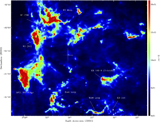
Figure 1.— $N_{\mathrm{H}_{2}}$ column density map of the W3 GMC corrected for contributions from foreground/background material. Labels mark prominent features in the cloud. The white cross marks the intersection of the four subfields in W3; counterclockwise from upper left: W3 Main/(OH), AFGL 333, KR 140, and W3 NW. The position of VES 735 is marked with a white X. The HDL is the dense region at the east comprising W3 Main, W3 (OH), and the AFGL 333 Ridge. Contours supplement the colorbar at the highest column densities, at $N_{\mathrm{H}_{2}}\approx[30,60,200]\times 10^{21}$ cm^-2.

In Paper I we used the column density map to investigate the nature of the most massive and highest column density structures. We found these structures to be most likely the result of feedback by high-mass stars, the combined, convergent effect of which might ultimately be responsible for the formation of the most massive Trapezium-like systems and clusters.

In this paper we present the second part of our Herschel analysis of the W3 GMC (Rivera-Ingraham, 2012; Rivera-Ingraham et al., 2013). Results below support the conclusion from Paper I that local stellar feedback appears to be a major player not only in the formation of clusters of high-mass stars but also in the overall process determining the characteristics and local evolution within a GMC.

In Section 2, we provide a brief introduction to the Herschel datasets and analysis techniques. Section 3 introduces the probability density functions (PDFs) and cumulative mass distributions (CMDs) and the procedure for selecting the structures associated with star formation. Appendix A discusses the effects of foreground/background (non-GMC) material on the analysis and Appendix B describes some details of the interrelationship between the PDFs and CMDs used. Section 4 embarks on the interpretation of structure. The results of our comparative analysis of the subfields in W3 are included in Section 5. Section 6 presents new evidence from the PDFs that could be used to trace and constrain the birthplaces of clusters of high-mass stars in a given region. We conclude in Section 7 with a summary of the key findings related to cloud structure and star formation properties of this cloud and how they relate to the results presented in our previous Herschel study of W3 regarding the high-mass star formation process.

2. Data Processing and Maps of Column Density

The W3 GMC was observed with Herschel (Pilbratt et al., 2010) as part of the HOBYS Key Programme (Herschel imaging survey of OB Young Stellar objects; Motte et al., 2010). In Paper I we presented the Herschel observations (SPIRE/PACS parallel scan ObsIDs: 1342216019, 1342216020; bright mode SPIRE ObsIDs (for saturation correction): 1342239797, 1342239796), ancillary data, and the techniques adopted to create and analyze maps of dust optical depth and temperature for this cloud. We recall that these maps were made by assuming a constant dust temperature along the line of sight and fitting spectral energy distributions (SEDs) pixel-by-pixel using the Herschel dust emission maps at wavelengths $\geq 160$  $\mu$m convolved to the resolution of the $500$  $\mu$m map ($\sim$36″; $\sim$0.35 pc at a distance of 2 kpc). To describe the SED we assumed a fixed dust emissivity index of $\beta=2$.

The optical depth and dust temperature maps were also corrected for the effects of emission from dust in the foreground/background of W3. This process removed the non-GMC components to reveal more closely the properties of the interstellar medium within the GMC. The correction was accomplished by estimating the contribution to the emission $I_{\nu}$ at each Herschel band from dust traced by atomic and molecular gas (H I and CO emission, respectively); see Rivera-Ingraham (2012) and Appendix B of Paper I for a detailed description of the steps and assumptions associated with this technique. This work uses these foreground/background interstellar medium (ISM)-corrected maps as the default for our analysis.

2.1. Alternative Representations of Column Density

To convert the observable, the dust optical depth, into gas column density, $N_{\mathrm{H}_{2}}$ (Figure 1), we assumed a dust opacity of 0.1 cm² gm^-1 at 1 THz and a mean atomic weight per molecule of $\mu=2.33$. The latter may be as high as 2.8 (Roy et al., 2013) but this slight inconsistency was retained here so that the column densities could be directly compared with results in other Herschel and HOBYS fields based on the same assumptions (e.g., André et al., 2010; Motte et al., 2010; Hill et al., 2011; Hill et al., 2012). While $\beta$ is not definitively known in molecular clouds and recent work points to opacity variations that should be considered (Roy et al., 2013; Planck Collaboration XI, 2014), none of these systematic uncertainties in scale should impact our results significantly, nor is such an investigation within the scope of this paper.

Many results in the literature relevant to the topic of this paper are given in terms of magnitudes of dust extinction $A_{\mathrm{V}}$ although that is not usually directly observable. For the purposes here we adopted the common approach of transforming $N_{\mathrm{H}_{2}}$ to $A_{\mathrm{V}}$ using $N_{\mathrm{H}_{2}}=0.94\times 10^{21}\thinspace A_{\mathrm{V}}$ cm^-2, although this is calibrated only for lower column densities and largely atomic lines of sight (Bohlin et al., 1978). Converting directly from submillimeter dust optical depth to $A_{\mathrm{V}}$ would seem more desirable/less contrived and indeed the challenges of doing this have been discussed (Planck Collaboration XI, 2014). However, again our conclusions here should not depend on these precise details.

For the corrected maps applying to the GMC material at a common distance of 2 kpc, we can convert the column density as parameterized by $A_{\mathrm{V}}$ into a mass per pixel: $M_{p}=f\thinspace A_{V}$. For the 9″ pixels used and the assumptions described above (distance to W3 and mean atomic weight per molecule) we find $f=0.13$ M_⊙ mag^-1.

3. Methodology: Identification and Characterization of Star-Forming Structures

To characterize the density structures in W3 we created PDFs of the column density maps and from these mass distributions.

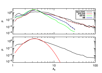
Figure 2.— Probability Density Functions (PDFs) in W3. The logarithmized version binned in $\log A_{\mathrm{V}}$ is plotted. Top: PDFs for each of four fields in W3. Errors bars are shown here as a reference. Bottom: Global PDF for the entire W3 GMC with a fitted lognormal function (red) and power-law tail.

PDFs quantify the fraction (or the probability $p$) of material in the cloud having a column density in the range $N_{\mathrm{H}_{2}}$ and $N_{\mathrm{H}_{2}}+\Delta$$N_{\mathrm{H}_{2}}$. PDFs have been used extensively as analytical tools for describing the distribution of mass in regions of low-mass star formation (e.g., Froebrich & Rowles, 2010; Kainulainen et al., 2009) and in regions of high-mass star formation as well (e.g., HOBYS studies: Hill et al., 2011; Schneider et al., 2012; Hill et al., 2012; Russeil et al., 2013).

The lower panel of Figure 2 shows the PDF for the entire W3 GMC. What is plotted is a “logarithmized” version of the PDF, $P\equiv P_{\ell 10}$, where the independent variable (for the binning) is now $\log A_{\mathrm{V}}$ (base 10).

The shape of PDFs is not always straightforward to interpret, as various physical processes imprint on its structure. For example, interstellar turbulence likely determines the lognormal distribution of low column-densities (see theoretical work of e.g., Klessen, 2000, and observations of Kainulainen et al., 2009 for all cloud types: quiescent, low-mass, and high-mass star-forming clouds). Following the approach used in previous studies, the main peak in the above PDF and those below was fitted with a lognormal distribution. All fits were carried out using a non-linear least-squares minimization idl routine based on mpfit (Markwardt, 2009) and the result plotted along with the underlying data.

External compression can cause a broadening of the PDF, as predicted in models of Federrath & Klessen (2013) and seen in Orion B (Schneider et al., 2013) and in clouds associated with H II regions (Tremblin et al., 2014). The shape of the PDF might therefore be used to infer concrete basic physical properties of the cloud and individual structures whose material is traced by the PDF (e.g., Fischera, 2014).

Of all processes, gravity plays the most important role at higher column densities and for low-mass star-forming regions causes a clearly defined power-law like tail in the PDF (Kainulainen et al., 2009; André et al., 2011; Schneider et al., 2013). High-mass star-forming regions often also show tails at high extinction that can also be accurately modelled as power-laws (NGC6334; Russeil et al., 2013). Such high-$A_{\mathrm{V}}$ tails can also have, however, more complex shapes as well, as has been found here within W3 and in other fields (see also Hill et al., 2011; Schneider et al., 2012). Indeed, processes such as turbulence, gravity, feedback/compression, magnetic fields, intermittency of density fluctuations, a non-isothermal gas phase, properties of the cloud formation processes, and even line-of-sight effects, could lead to complex substructure in the PDF tails, such as “breaks” and peaks, that might not necessarily be well represented with a simple power-law function. In the next sections, we will discuss in more detail how stellar feedback might also imprint on the PDF shape. Effects on the PDFs produced by contamination from foreground/background material along the line of sight, avoided here, are described briefly in Appendix A.

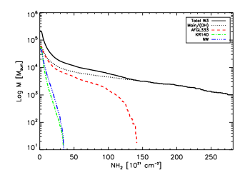
Figure 3.— Cumulative mass distributions for the W3 field (black: solid line) and for each of the four fields: W3 Main/(OH) (black: dotted line), AFGL 333 (red), KR 140 (green), and W3 NW (blue). The column densities $N_{\mathrm{H}_{2}}$ can be compared directly with Figure 1. In terms of $A_{\mathrm{V}}$, the x-axis range is very similar, 0 to 320 mag.

Column densities theorized in other studies to be associated with high-mass star formation are very high, for example $\Sigma=0.7$ g cm^-2 to produce a star with $M\sim 10$ $M_{\odot}$; Krumholz & McKee, 2008, which corresponds to $N_{\mathrm{H}_{2}}\sim 180\times 10^{21}$ cm^-2 or $A_{\mathrm{V}}\sim 200$ in our maps and PDFs therefrom. Cloud column densities of this order, typically observed only towards regions of active high-mass star formation, are rare and therefore there are often poor statistics at the high extinction end of PDFs. In our explorations we found that the cumulative form of the mass distribution, the CMD (i.e., the total mass above any given magnitude; e.g., Froebrich & Rowles, 2010), allows for a complementary and often more straightforward analysis of the higher end of the PDFs.

The large differences between neighboring regions in W3 (e.g., the dense and active HDL vs. the more quiescent and diffuse western fields; Rivera-Ingraham et al., 2011; Paper I) make it necessary to quantify how in-cloud local conditions affect the star formation process. To this end, we have carried out an analysis of individual areas within W3 itself, these being the four fields into which we divided this cloud in Paper I: the W3 Main/(OH), AFGL 333, KR 140, and W3 NW fields (Figure 1).

The PDFs of each of the four fields in W3 are given in the upper panel of Figure 2; the characteristics of the global PDF of W3 in the lower panel clearly depend on the contributions from each of the four fields.

Figure 3 shows the corresponding CMDs, very different for the four fields. In this figure this is expressed in terms of $N_{\mathrm{H}_{2}}$ for more direct comparison with the high column density regions in Figure 1.

4. PDF Interpretation and Clues to Cloud Structure

Table 1Breaks and Parameters for Linear Fits to the CMDs

Field	Mass	Break1	Break2	Slope/Intercept (1)	Slope/Intercept (2)	Slope/Intercept (3)
	(104 $M_{\odot}$)	(mag)	(mag)
Main/(OH)	$6.0$	13.0	38.5	-0.0469/+4.8823	-0.0154/+4.4656	-0.0032/+3.9958
AFGL 333	$6.3$	6.0	22.5	-0.0920/+5.0419	-0.0360/+4.7095	-0.0084/+4.0903
KR 140	$5.9$	6.5		-0.2120/+5.3082	-0.0945/+4.5196
W3 NW	$4.8$	6.0		-0.1465/+5.0572	-0.0844/+4.6769

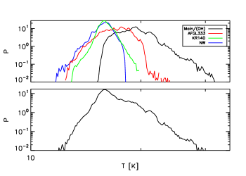
Figure 4.— Like Figure 2 but for the logarithmized PDF of dust temperature. Top: for each field in W3. Bottom: global PDF of the W3 GMC.

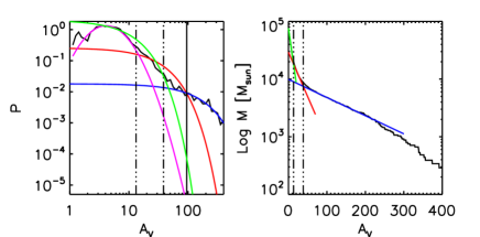
a W3 Main/(OH) field

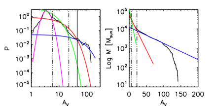
b AFGL 333 field

Figure 5.— PDFs (left) and CMDs (right) for the two fields in the (eastern) HDL. CMDs: Solid green, red and blue lines are the best linear fits to the data. Vertical dash-dotted lines mark the breaks in the distribution ($A_{\mathrm{V}}$(SF) and $A_{\mathrm{V}}$(HTB); see text). PDFs: Vertical dash-dotted lines and green, red, and blue curves are those derived from the CMD (Appendix B). Magenta curve is the best-fit lognormal function to the PDF peak. Solid vertical lines are $A_{\mathrm{V}}$(HB), where the flatter components start to dominate.

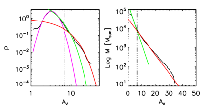
a KR 140 field

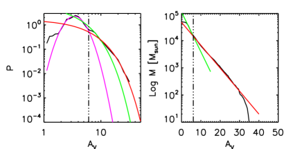
b W3 NW field

Figure 6.— Same as Figure 5, but for the two western fields. These two fields lack the flattening of the PDF at high extinction that characterizes the HDL fields.

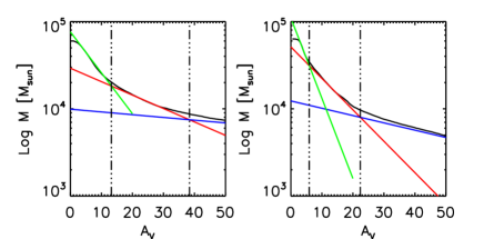
Figure 7.— Expanded view of the low extinction range of the CMDs in Figure 5, highlighting the breaks and the best linear fits to the data for W3 Main/(OH) (left), and AFGL 333 (right).

4.1. Analysis and Characterization of PDF Substructure

While various factors can influence the shape of a PDF, the column density above which it deviates from a lognormal distribution into a power-law (i.e., the break) has been commonly interpreted as the point separating the turbulent medium from the star formation regime. The PDF break can therefore be understood as the column density above which star-forming structures start to dominate over the local environment (e.g., Kainulainen et al., 2009; André et al., 2011; Ballesteros-Paredes et al., 2011 and references therein).

This break is therefore an essential parameter for constraining the star formation properties of individual fields. We have found that such breaks can be identified and characterized by fitting linear functions to the $\log$ of the CMD. See Rivera-Ingraham, 2012 and Appendix B for a more detailed description of the concepts and methodology used. Although the accuracy of the estimate of the break can be affected by the binning ($\Delta A_{\mathrm{V}}=0.5$ mag) and fitting procedure (uncertainties in linear slopes are $\sim 5$ %), a major source of systematic uncertainty for the lowest breaks will arise from the corrections applied to the maps to remove line-of-sight, non-GMC material, as explained in Appendix A.

In our application of this approach, the division into subfields from Paper I was used, as it separates regions with dramatically different characteristics. Our choice of subfields was determined by unique differences in column density and temperature distributions, stellar activity, and stellar content. Constraining the origin of these differences is crucial for understanding the onset of high-mass star activity in the very specific regions of the HDL. The temperature differences can clearly be observed, for instance, in the temperature PDFs for each field in Figure 4. The W3 Main/(OH) field is the most active and warmest, as well as the only one with ongoing high-mass star formation. At the other extreme, the KR 140 and W3 NW fields are cold and quiescent. The AFGL 333 has intermediate properties, with some high-mass stars, and yet is much more quiescent than W3 Main/(OH).

The derived values and parameters for the linear fits (slope and intercept of the lines used to represent the mass distributions) are given in Table 1 and the fitted lines are shown in the right panels of Figures 5 and 6. An expanded view of the CMDs in Figure 5 has been included in Figure 7.

The Figures show that the first breaks ($A_{\mathrm{V}}$(SF)) derived from the mass distributions approach those in the PDFs, while the shapes of the components can effectively account for visual changes (bumps) in the tails of the PDFs. The accuracy for determining the break clearly depends on the sharpness of the transition between the different (linear) regimes in the mass distributions (i.e., those fitted with linear functions). A slow transition between two regimes (i.e., not sharp, but progressive and occurring over a broader extinction range, as observed for those in the HDL; Figure 7) would result in a higher degree of uncertainty, as the identification of the end and starting points of the linear regimes becomes less clear. A higher degree of uncertainty for the first break of the KR 140 field is expected due to this effect and the fact that this field is also the one with the most severe line-of-sight (molecular) contamination.

Prominent differences can be seen between the PDFs of the two regions in the HDL and those of the western fields. W3 NW and KR 140 (see Figure 6) show simpler, well-fitted PDFs. While a classical power-law function would not be able to reproduce the PDF tails of the western fields, our fits derived from the linear functions to the mass distributions can reproduce them well. The W3 Main/(OH) and AFGL 333 fields (see Figure 5) have much more complex tails extending to high extinction. While our fits do not manage to reproduce this complexity as accurately as those for the western fields, they successfully locate the $A_{\mathrm{V}}$(SF) break and manage to trace the overall variation of the tails with increasing extinction. Note that, like for the western fields, the tails of these PDFs would not be well fitted with a classic power-law function either.

The fits to the mass distributions reveal the presence of a second major break in the PDFs of the HDL fields (defined in this work as $A_{\mathrm{V}}$(HTB), for “High-extinction Transition Break”). This break marks the transition point between the classical power-law tail of the PDF and a “flatter” regime, fitted in the mass distributions with a third linear function (blue slopes; Figure 5). As with the first break in the KR 140 field, this second transition was found to be considerably wide and progressive (i.e., characterized by a smooth, slow transition) for both HDL fields, therefore resulting in a higher degree of uncertainty when determining the true transition point. The regions traced by these intermediate (transition) extinctions are identified with the structures and shells in W3 Main/(OH) and the AFGL 333 fields, which host the most massive ridges and clumps in the W3 GMC.

The actual break at which the flat regime at high extinctions starts to dominate in the PDF ($A_{\mathrm{V}}$(HB)) is marked by the point where the mass distribution is properly described by the third linear function, whose parameters have been included in Table 1. This extinction is also coincident with the point where the two linear fits (blue and red) in the mass distributions intersect in the PDF (Figure 5). These points are $A_{\mathrm{V}}$(HB)$\sim 45$ mag and $95$ mag for AFGL 333 and W3 Main/(OH), respectively. The presence and nature of this possible break is important due to its link with high column density material, including high-mass star-forming regions.

4.2. Interpretation and Clues to Cloud Structure

While all fields have comparable total mass, those in the HDL have distributions of material at higher extinctions that distinguish them, not only from the KR 140 and W3 NW fields, but also between themselves (e.g., based on Kolmogorov-Smirnov (KS) probability tests). Considering also their dramatic differences in (high-mass) stellar activity, characterization of the different $A_{\mathrm{V}}$ regions, with the aid of the PDFs, is essential for understanding the processes driving current star formation and the history that led to these (successful) conditions. Below, we discuss each $A_{\mathrm{V}}$ range in turn.

4.2.1 Low $A_{\mathrm{V}}$ Range: Constraining Environmental Conditions

Compared with other high-mass star-forming regions (e.g., Rosette cloud; Schneider et al., 2012), the properties of the PDFs/mass distributions of W3 indicate that material with extinction $A_{\mathrm{V}}\sim 3$ mag comprises a typical GMC environment, or common plateau, on which the structures with star-forming potential are observed. Note that the critical extinction for core formation of $A_{\mathrm{V}}\sim 8$ mag (André et al., 2010) relies on a filamentary environment, so the above estimate represents the environment of the filament itself.

Excluding W3 Main/(OH), the only field with confirmed on-going high-mass star formation (e.g., HC H II regions), the actual transition point to the gravity-dominated regime in W3 is found to be $<$$A_{\mathrm{V}}$(SF)$>\approx 6$ mag. More than $90\thinspace\%$ of the Class 0/I YSO population (Rivera-Ingraham et al., 2011) is contained above the $A_{\mathrm{V}}$(SF) of a given field (except in KR 140, where $\sim 30\thinspace\%$ of the population is below the $A_{\mathrm{V}}$(SF)). The PDF breaks are therefore suitable limits for identifying the major current and potential star-forming sites in the GMC, separating these from typical environmental column densities in the cloud. The amount of star-forming cloud mass in each field, based on these limits, is shown in Table 2.

Similarly, we can also define typical environmental temperatures, or $T_{\mathrm{env}}$, for each field. The temperatures associated with material below the $A_{\mathrm{V}}$(SF) coincide with the peaks of the temperature PDFs shown in Figure 4; i.e., $T\approx 19.5$ K, $17.5$ K, $16.0$ K, $16.0$ K for W3 Main/(OH), AFGL 333, KR 140, and W3 NW, respectively. Note, however, that a key property of the youngest high-mass star-forming regions in W3 is their association with high-column density material with temperatures highly above environmental (Paper I). Exclusion of such warm material when identifying young regions would clearly underestimate the true star-forming potential of the GMC, especially in terms of high-mass stars.

Table 2Characteristics of On-going and Potential Star-forming Structures

string$M$stringstring	%string	$<T>$string	Areastring	%string
($10^{3}$ M⊙)		(K)	(pc2)
W3 Main/(OH)
$20.5\pm 0.12$	34.2	$21.1$	39.8	7.6
$4.9\pm 0.04$	8.2	$18.3$	11.1	2.1
AFGL333
$34.1\pm 0.09$	53.9	$17.1$	151.1	24.7
$19.8\pm 0.07$	31.3	$15.5$	80.4	13.1
KR140
$9.5\pm 0.03$	16.2	$15.5$	59.4	6.6
$7.3\pm 0.03$	12.4	$15.1$	42.9	4.7
W3 NW
$15.9\pm 0.04$	32.8	$15.0$	97.6	15.2
$14.9\pm 0.04$	30.7	$14.8$	89.4	13.9

4.2.2 High $A_{\mathrm{V}}$ Range: Searching for Sites of High-Mass Star Formation

Characterizing the nature of the second break at high $A_{\mathrm{V}}$ in the PDFs is crucial due to its possible association with regions of high-mass star formation. While similar breaks were also observed by Schneider et al. (2012) for the Rosette field containing the highest column densities (reaching $A_{\mathrm{V}}\sim 70$ mag in their maps), the AFGL 333 and W3 Main/(OH) fields reach extinctions 2-6 times this limit, and second breaks about 2.5-4.5 that observed in Rosette. In the following sections, we suggest that these second breaks originate from, or are influenced by, the effects of an external dynamic process. In the case of W3, this process is dominated by stellar feedback and associated triggering (compression) from high-mass stars, acting on already relatively dense star-forming structures (e.g., shells). Therefore, the structure of the PDFs of W3 provide additional evidence for the convergence constructive feedback scenario of high-mass star formation (Paper I).

5. Discussion: Favorable Conditions for High-Mass Star Formation

The W3 GMC offers a unique opportunity to investigate star formation under different environmental conditions, from high density structures with high stellar feedback (eastern HDL), to more diffuse and quiescent (western) regions with localized star formation (Rivera-Ingraham et al., 2011). In the following sections we compare the fields in W3 to constrain the conditions that have led to the (rare) onset of high-mass star formation in this GMC.

5.1. The Environmental Factor $A_{\mathrm{V}}$(SF) and the Role of Stellar Feedback in Determining Local (in-Cloud) and Global Evolution

The HDL, hosting the only young high-mass population in W3, comprises up to $\sim 70\thinspace\%$ of the dense (above environmental limit; $A_{\mathrm{V}}$(SF)) material in the GMC. For comparison, W3 Main/(OH) and AFGL 333 contain up to $\sim 2.5$ times more mass for potential star formation than the neighboring western fields KR 140 and W3 NW.

Assuming that a third of the total mass of W3 with $A_{\mathrm{V}}>$$A_{\mathrm{V}}$(SF) is transformed into stars (Alves et al., 2007), the HDL would therefore have a total mass fraction involved in star formation (Mass_SF; or “MSF” in Froebrich & Rowles, 2010) of $\sim 15$ % at a resolution of $\sim 0.35$ pc (c.f. the western fields: $Mass_{\mathrm{SF}}\sim 7.5$ % of their total mass $M_{tot}\sim 1.1\times 10^{5}$ $M_{\odot}$). The W3 GMC as a whole shows a Mass${}_{\mathrm{SF}}\approx 11.5$ %.

While the mass of the W3 GMC is comparable to that of Auriga 1 or Cepheus, these clouds only have Mass_SF of just 0.19 % and 0.26 %, respectively (Froebrich & Rowles, 2010). The maximum Mass_SF found by Froebrich & Rowles (2010) (in their cloud sample) is $\sim 10$ % (Corona Australis). Compared to these low-mass star-forming clouds, W3 appears to have an anomalously high proportion of mass involved in star formation, with a very high potential to form new stars in the next $10^{6}$ yrs (Froebrich & Rowles, 2010) despite its already significant ongoing star activity.

W4 shows signatures of prominent stellar activity that has been ongoing for at least $\sim 6-20$ Myr (Oey et al., 2005). Regardless of the distribution of material in the W3 region prior to the formation of W4, the scenario of successive episodes of (high-mass) star formation and bubble development described by these authors suggests that W4 not only influenced the star formation process in W3 at the distance of the HDL, but also that the HDL, the densest structure in W3, originated due to this same activity of bubble/shell expansion, redistribution, and compression of material. The idea of a triggered origin for the HDL (e.g., by compression) has already been suggested in previous studies (e.g., Moore et al., 2007), and is strongly supported by extensive observational evidence. Its location, parallel to the W4 H II region, the morphological and physical characteristics of the HDL presented in this work, as well as the W4-W3 stellar age and cluster distributions (e.g., Carpenter et al., 2000; Rivera-Ingraham et al., 2011), indicate a clear influence of W4 on the material as well as the stellar activity in the HDL over an extended period of time. Based on this result, and with the HDL dominating the contribution of dense material in the GMC, stellar feedback can therefore explain the high Mass_SF in the HDL and therefore in W3 as a whole. Feedback as the driver distinguishing the structures in the HDL from those in the western fields is also supported by molecular observations (Polychroni et al., 2012). The key issue remains as to whether or not feedback can also explain the local differences between fields, and why high-mass star formation is exclusive to just some particular regions in the HDL (W3 Main/(OH)).

Theoretical models and simulations predict that stellar feedback can indeed have a significant impact on the star formation process. Depending on environmental conditions and the location and number of high-mass stars, feedback strongly disturbs cloud morphology, shifting and redistributing material and creating new dense regions potentially suitable for low and high-mass star formation alike (e.g., Whitworth et al., 1994; Dale et al., 2007; Walch et al., 2013). It can also affect the average stellar mass, by dispersing or concentrating the local material needed for accretion, while increasing the total number of young stars of a given region (e.g., Federrath et al., 2014; Dale et al., 2015). Its effects on local star formation from winds and (especially) ionization (e.g., Dale et al., 2013) are, however, dependent on distance and environmental density, with its destructive effects being highly minimized in the densest environments (e.g., Dale & Bonnell, 2011; Ngoumou et al., 2015). Ultimately, feedback might regulate the global star formation process at a range of spatial scales through the input of turbulence (e.g., Klessen et al., 2004; Boneberg et al., 2015) and a complicated balance between destructive (e.g., material dispersal) and constructive effects (e.g., compression, material accumulation and creation of dense structures; e.g., Dale et al., 2007; Krumholz et al., 2014 and references therein).

Based on our observations and the general theoretical predictions in the above studies, we suggest that stellar feedback from high-mass stars is currently the main factor distinguishing the observed differences in star formation between fields in the W3 GMC, disrupting the local environment and altering the characteristics, onset, and evolution of the star formation process in a given region. This effect can be inferred from Table 3, which summarises the environmental differences between W3 YSO populations. Here we used the $N_{\mathrm{H}_{2}}$ and $T$ of the pixel in the Herschel maps coincident with the YSO coordinates as representative of the local conditions in which a given YSO resides (pixel size$\sim$0.1 pc).

Table 3Average Environmental Properties of YSOs in the W3 GMC.

stringYSOsstringstring	$<T_{d}>\phantom{string}$	$<A_{\mathrm{V}}>$string
	(K)	(mag)
W3 Main/(OH) + AFGL 333
All types	18.1	$25.6$
Class 0/I	16.9	$56.6$
Class II	18.5	$14.8$
KR 140 + W3 NW
All types	15.3	$9.1$
Class 0/I	14.8	$12.9$
Class II	15.5	$7.9$

The mean extinction of Class 0/I and Class II candidates in the HDL (Rivera-Ingraham et al., 2011) is $A_{0/I-HDL}>4.4\times A_{0/I-West}$ and $A_{II-HDL}\approx 1.9\times A_{II-West}$, respectively (Table 3). The triggering process that originated the HDL, in combination with the activity from the local high-mass stars in W3, have therefore provided the denser (and warmer) conditions suitable for the onset of the most vigorous and richest stellar activity currently observed in the W3 GMC.

Similarly, comparison of the local differences between Class 0/I and Class II YSOs in a particular region ($\Delta$$<A_{\mathrm{V}}>$, or the change in local column density with time), can constrain possible environmental effects on YSO evolution. Assuming a total lifetime for the Class 0/I (+flat SED) and Class 0/I + Class II phases of $\sim 0.9$ Myr and $\sim 2.9$ Myr, respectively (Evans et al., 2009), then for co-eval evolution (same age) Class II YSOs in the HDL could leave or have their environment disrupted (e.g., higher external activity) up to $\sim 8$ times faster than in the western fields, whose Class 0/I and Class II candidates co-exist in similar (cool) environments and comparable column densities. In a more conservative scenario in which Class II sources in the HDL are the oldest (2.9 Myr old) Class II population in W3 (while those in the western fields have just been formed; i.e., 0.9 Myr old), then Class II sources in the HDL still dissociate from their primordial material $\sim 2.5$ times faster than those in the western fields. According to theoretical models, this apparently negative effect could result in the new stellar population in the proximity of the high-mass stars in the HDL being more numerous, albeit with overall lower masses than the more localized stellar population formed in the more quiescent western fields. The HDL has, however, a significant high-mass star population and massive clusters whose origin might also be linked to the (in this case, constructive) effects of triggering and external events (Paper I).

Below we summarize the observational evidence from this work supporting a feedback-driven model for the local evolution of regions within the W3 GMC. These results aim to introduce the basis of a scenario (Section 5.2) in which evolution is intimately linked to the balance of constructive/destructive effects of the feedback mechanism, themselves highly dependent on local environmental density.

5.1.1 The HDL: Star Formation in Very High-Density Environments

W3 Main/(OH) is the only field with ongoing (clustered) high-mass star formation, despite the fact that the AFGL 333 is also influenced by the activity in W4. Considering the effects of stellar feedback on star/structure formation, this intense star formation, as well as the other unique properties of the W3 Main/(OH) field, might ultimately be linked to its particularly high degree of stellar feedback from current stars within W3 on a quite local parsec scale (a few arc minutes on Figure 1), including but certainly not exclusively high-mass stars in IC 1795 and those powering W3 Main. This appears to the dominant mechanism distinguishing the current state and evolution of the different fields. The key role of local high-mass stars acting already within the W3 complex, rather than external activity from W4, for determining the current conditions of the star-forming material within dense environments is based on the following observations:

1) W3 Main/(OH) has more extreme environmental conditions, with a $T_{\mathrm{env}}$ higher than that observed for AFGL 333. This would be inconsistent with the activity in W4 being a main factor determining the in-cloud state of the HDL, as the latter is closer (in projection), and more heavily irradiated by, the high-mass stellar activity in W4. We find that $>95\thinspace\%$ of the AFGL 333 field is below the $T_{\mathrm{env}}$ of W3 Main/(OH), excluding the pillar east of the AFGL 333 Ridge (YSO Group 7; Rivera-Ingraham et al., 2011), and IRAS 02245+6115, an H II region associated with a B-type star (Hughes & Viner, 1982; Straižys & Kazlauskas, 2010).

2) W3 Main/(OH) has a much more significant (and on-going) stellar activity (Rivera-Ingraham et al., 2011), as well as a higher disruption of the YSO environment. About $\sim 80\thinspace\%$ of Class II sources with $A_{\mathrm{V}}\leq$ $A_{\mathrm{V}}$(SF) also have $T>T_{\mathrm{env}}$ in this field.

3) While both HDL fields reach column densities of the same order, W3 Main/(OH) also has a PDF break $A_{\mathrm{V}}$(SF) twice that of the AFGL 333 field. This higher break selects the shell-like structures around IC 1795, shaped by the central cluster and its (parsec-scale) feedback from local high-mass stars (Rivera-Ingraham et al., 2011). In addition to gravitational effects, this PDF break could therefore be directly influenced by the magnitude of external/active processes.

If dynamic (e.g., feedback) processes are key for anomalously enhancing the amount of star-forming (dense) material in W3, shifting the position of the PDF break, and driving the high-mass star/cluster formation itself (as suggested in Paper I), then this common link could, in addition, explain why: i) W3, a high-mass star-forming cloud, has a higher Mass_SF than any of the low-mass star-forming clouds in the sample of Froebrich & Rowles (2010), and ii) fields classified as high-mass star-forming regions have generally a higher $A_{\mathrm{V}}$(SF) than low-mass star-forming regions (as observed in, e.g., Schneider et al., 2012).

5.1.2 The Western Fields: Star Formation in More Diffuse Environments

In the KR 140 field, material with $A_{\mathrm{V}}>$$A_{\mathrm{V}}$(SF) is exclusively related to filamentary and shell-like structures; i.e., the Trilobite, the shell of the KR 140 H II, and the West Loop. (Figure 1). Each of these structures has a morphology consistent with external influence: Radiative-Driven Implosion (RDI; Rivera-Ingraham et al., 2011), the shell around the O-type star VES 735, and the border of a cavity-like structure observed in the CO map from the Canadian Galactic Plane Survey (CGPS; Taylor et al., 2003) at $v\approx 49.3$ km s^-1, respectively. The triggered-like origin of these structures is supported by the (asymmetric) distribution of their YSO population (Rivera-Ingraham et al., 2011), and column density and temperature profiles (e.g., asymmetric gradients). A profile example for the Trilobite can be seen in Figure 8.

The comparison between the two western fields resembles that between AFGL 333 and W3 Main/(OH), albeit in a much smaller scale. A possible cluster in the central-southern parts of the western fields (M. Rahman, priv. comm.) might have led to a period of enhanced feedback in the KR 140 field, resulting in higher feedback and a richer stellar content than in W3 NW; e.g., embedded clusters (Carpenter et al., 2000), various (late) B stars (Voroshilov et al., 1985), and the only (confirmed) O-star (VES 735) outside the HDL (according to SIMBAD). This affected the temperature distribution accordingly, with KR 140 having a much smaller proportion of “cold” material in any given extinction range than the W3 NW field.

The western fields therefore provide observational evidence of a radically different evolutionary path with respect to those in the eastern layer. Based on their properties relative to those of the HDL, such evolutionary difference could be easily linked to differences in the level and type of feedback in the history of W3 NW and KR 140. Here, structures have not benefitted from the primordial dense conditions provided by the external feedback that the first episodes of star formation in W4 provided for the eastern side of W3. Similarly, they also lack major sources of local internal feedback comparable to that of the HDL. Indeed, compared to the HDL, the localized star formation and the much lower level of local feedback in the western fields could also explain the low $T_{\mathrm{env}}$ of KR 140 and W3 NW as a whole, as well as the lack of a second break in their mass distributions.

Figure 8.— Profiles 200″ ($\sim 2$ pc) long through the column density peak of the Trilobite centered on position RA/Dec: $2^{\mathrm{h}}$ 21^m 5.^s3, +61^∘ 27′ 29.^′′1. Both temperature (dashed line; right scale) and column density (solid line; left scale) are shown for different orientations of the profile: in the West-East direction (top-left); NW-SE (top-right); North-South (bottom-left); NE-SW (bottom-right). Black vertical line marks the coordinate center (solid line).

5.2. The Herschel View of the Star Formation History and Evolution of the W3 GMC

Arising from this work is compelling observational evidence of the dramatic effects that stellar feedback can have on the evolution of a cloud. Initially, dense structures with conditions particularly favorable for new star formation can be created by local (in-cloud) or, in the case of the HDL, external feedback effects. These initial (past) conditions determine the properties of the first and subsequent episodes of star formation and associated local feedback events. The cumulative effects of this sequence of events will ultimately determine the general state of the region at the current epoch being observed.

Quantifying the balance between destructive/constructive effects of stellar feedback, influencing (opposing or aiding) known physical processes associated with star formation, such as self-gravity, accretion, and turbulence, is therefore fundamental for understanding the star formation process itself, from cloud to galactic scales. Our Herschel-based results can be used as observational constraints to construct a coherent evolutionary model of the W3 GMC, and therefore of the conditions and processes that ultimately originate the exotic high-mass stars and clusters.

Past studies indicate that star formation in the western fields must have been initiated at the same time as (if not before) the HDL (e.g., Rivera-Ingraham et al., 2011). Results from the present work suggest, in addition, that the main difference between the evolution and properties of the structures and stellar population of the different fields might be the magnitude of the local stellar feedback occurring within those fields. This difference in feedback level can, however, itself be linked to the primordial amount of mass and mean density in these fields, and therefore the initial level of star-forming activity.

A lower initial star formation efficiency (SFE) in a relatively low density medium would result in lower efficiencies for inducing star formation in secondary events, and a lower likelihood in compressing an already low column density medium to create structures dense enough for high-mass star formation. While this local compression might still result in few, relatively isolated, high-mass stars (e.g., KR 140) and some localized star formation (Rivera-Ingraham et al., 2011), the limited secondary star formation and low environmental column densities ultimately restricted the star formation capability of the western fields to a relatively low level.

The situation in KR 140 and W3 NW differs from the self-enhanced process in regions with initially enhanced column densities, like the HDL. Such a set-up would promote an initially high SFE, resulting in more intense (constructive) compression and triggering events. When acting on an already dense environment, this process would lead to the formation of new high-mass stars, as well as a richer stellar population (e.g., Dale et al., 2007). In turn, this population would then be more effective in further compressing and confining nearby material and therefore further enhancing the star formation activity.

Our conclusions would agree with the results of Carpenter et al. (2000), who found that embedded clusters in the W3 region are preferentially located in triggered regions. The evidence presented in this work also resembles the “fireworks hypothesis” presented by Koenig et al. (2012). In that model, the stellar feedback by high-mass stars triggers the formation of richer stellar populations, a self-propagating mechanism that can spread through the formation of new generations of high-mass stars when dense material is available. In W3, we suggest that this process occurs not only due to the original prime conditions created by W4 (i.e., the HDL), but also due to the generations of high-mass stars themselves, which continue creating the conditions needed for the formation of new populations of low-mass and, especially, high-mass stars and massive clusters.

The mechanism that we invoke for high-mass star formation in dense environments, and more particularly, for W3 Main, was first introduced in Paper I. In our proposed scenario, stellar feedback creates new dense material, but the properties of the high-mass star population and subsequent triggering events, taking place within an already triggered and therefore density-enhanced region, ensures that the new dense structures are also (high-mass) star-forming ones. This is achieved in part due to the active process of mass assembly and confinement of the triggering mechanism, that allows for the continuation of the star-forming process. We note that this differs dramatically from the scenarios presented in theoretical models (e.g., Dale et al., 2015). In these models feedback by O stars creates dense material, but this material is incapable of forming stars efficiently because it is expelled from the potential wells that facilitate collapse. Similarly, stellar feedback has been predicted in some cases to lower the mass of the new stellar population by dispersing local material and disturbing accretion, (e.g., Federrath et al., 2014). While more detailed simulations are required to test the specific scenario described here at sub-parsec scales, our observations suggest that the triggering conditions and the dense environments can enhance the availability of material and aid the accretion process. The combined effects would ultimately lead to the unique population of high-mass stars and clusters in W3 Main.

Star formation in W3 Main started and progressed independently from other regions (Feigelson & Townsley, 2008; Rivera-Ingraham et al., 2011). In the former, star formation was subsequently enhanced by the on-going low-mass activity and the local (but large scale - several parsec) triggering effect from IC 1795 (Figure 1; age $\sim 3-5$ Myr; Oey et al., 2005; Roccatagliata et al., 2011), itself created by the original superbubble activity in W4 (e.g., Oey et al., 2005). This process led to the first generation of high-mass stars in the shell around this cluster, which ultimately led to the onset of the convergent constructive feedback in W3 Main (Paper I).

6. $A_{\mathrm{V}}$(HB), the Second Break in the CMD/PDF: Tracing the Origin of the Birthplaces of Clusters of High-Mass Stars

A second break in the mass distributions is a property unique to the HDL fields. In this case, that of the W3 Main/(OH) field ($A_{\mathrm{V}}$(HB)$\sim 95$ mag) is observed to be at an $A_{\mathrm{V}}$ twice that of AFGL 333.

Column densities above the $A_{\mathrm{V}}$(HB) breaks are associated exclusively with the two high-mass star-forming regions W3 (OH) and W3 Main, and the AFGL 333 Ridge, the only one of the three without confirmed high-mass star formation. While a lack of high-mass stars in AFGL 333 might be due to a younger age (e.g., Sakai et al., 2007; Polychroni et al., 2012), the fact that the mass in the AFGL 333 Ridge above its $A_{\mathrm{V}}$(HB) covers an area equivalent to the area above the same extinction in the three clumps in W3 Main/(OH) combined, suggests that the lower number of high-mass stars and their farther distance from the forming structure might have led to lower densities and a smaller degree of compression and confinement.

We observe that all the structures traced by the $A_{\mathrm{V}}$(HB) contour coincide with those we identified in Paper I as most likely associated with a dynamic input of material. When acting on a region with already enhanced column densities (like the HDL or the shell around IC 1795), boundary high-mass stars can be particularly efficient with sub-parsec triggering (e.g., AFGL 333 and W3 Main). If the second break in the PDF traces those structures associated with such dynamical processes (feedback-dominated in the case of the W3 GMC, in addition to any additional gravitational inflow of material from the local neighborhood this amount of mass might ultimately induce), then this feature in the PDF could act as a signpost for locating structures with enough mass at high extinction for possible high-mass star formation. Note, however, that having the potential for forming high-mass stars might not necessarily translate into actual high-mass star formation itself, as this might occur only under very specific conditions (as discussed in Paper I). Similarly, the actual $A_{\mathrm{V}}$ at which the second break occurs might vary from region to region, depending on factors such as local environment, strength, and direction of the triggering event (e.g., AFGL 333 and W3 Main).

Our results link the presence of a high-extinction break in the PDF with the effects of an external (dynamic) effect. Based on our observations, stellar feedback appears to be the major dynamic process acting within and on W3, which is the reason why feedback has been specifically mentioned and referred to in our discussion as the major driver in the evolution of W3. This stellar feedback-based constructive process could also be applicable to other regions (e.g., Xu et al., 2013). In more general terms, conclusions from this work in terms of high-mass star formation requirements would hold when stellar feedback is replaced or aided by other external events capable of recreating similar conditions. This would be in agreement with the conclusion from the HOBYS study of Vela C by Hill et al. (2011), who suggested that the flat part of their PDFs could be the result of constructive large scale flows. Like the convergent constructive feedback mechanism introduced in Paper I, convergence of flows could indeed also satisfy the requirement of an active input of material that in Paper I we suggested could be the key to high-mass star and cluster formation. A study of the applicability of this scenario to other regions within the Galaxy, and its associated observational evidence (e.g., PDFs), is currently the focus of ongoing work (Rivera-Ingraham et al. 2015; in prep.).

7. Conclusions

The W3 GMC offers a unique opportunity to investigate the formation process in a variety of environments. In this second study of W3 with Herschel HOBYS data, we have aimed to create a coherent picture of the evolution of this GMC, analyze its large-scale properties and structure, and further constrain the high-mass star formation process as first described in Paper I. This study has been carried out by means of a comparative analysis of the fields in W3 based on the properties derived from the Herschel column density and temperature maps.

The W3 Main/(OH) and AFGL 333 fields show a second break in their mass distributions. This break appears to be related to the presence of external dynamic processes acting on the observed structures. Since this influence is the suggested major mechanism for forming the most massive clusters of high-mass stars (Paper I), this break could act as an effective signpost for identifying regions suitable for possible high-mass star formation. The actual location of this break will depend on the local environmental conditions.

While the first break of the PDF is expected to be influenced by various factors (e.g., gravity), we have presented evidence that dynamic processes such as external feedback can also be responsible for altering the location of this break. If such processes are major players in both shifting the break in the PDF and high-mass star formation itself (Paper I), then it could explain why high-mass star-forming regions have a tendency to have a higher break than low-mass star-forming regions, as observed in previous studies.

The combined evidence provided by the YSO population and the Herschel datasets suggest that differences in the primordial local conditions are key for determining the evolution and current structural and stellar properties of each field. A high initial surface density, mass, and column density could allow for a higher initial SFE. The combination of a high SFE acting in an already high density region (like the HDL), combined with the properties of triggering as a star formation process, could result in a self-enhancing process in which subsequent triggering events lead to an increase of the very structures suitable for further star formation. This picture is supported by the anomalously high proportion of star-forming material in W3 as traced by Herschel, compared to other low-mass star-forming clouds. The same events could then lead to a richer population, a fireworks hypothesis as suggested by Koenig et al. (2012), as well as more massive stars. The particularly enhanced local large scale feedback observed for the W3 Main/(OH) field could therefore explain why this is the only field with significant high-mass star formation.

The western fields on the other hand show only moderate stellar feedback. This state would be commonly associated with the quiet evolution of a cloud lacking the atypical conditions provided by W4 and the HDL, which have greatly enhanced the star-forming potential of the eastern regions of W3.

The combined effectiveness of feedback and similar dynamic processes (e.g., constructive convergence of flows) in 1) the creation of column density structures suitable for star formation (as shown in this work), and 2) star formation itself (as suggested in previous studies), could then support the scenario where star formation progresses simultaneously with the formation of their parent structures. This process would translate into an increasing energy output (luminosity) of a star-forming structure (e.g., core/clump) as the structure itself is assembled (equivalent to a diagonal evolution in the L/M diagram). Such a model matches the scenario introduced with the convergent constructive feedback process in Paper I.

Appendix A Effects of (non-GMC) Foreground/Background Material on Column Density and PDFs

While the use of the column density maps corrected for foreground/background material can be properly described with a single lognormal distribution, it was observed that the use of ISM-uncorrected maps resulted in a secondary peak at low extinctions ($A_{\mathrm{V}}\approx 2.5$ mag) for the two northernmost fields (W3 Main/(OH) and W3 NW, and therefore also on the global PDF of the GMC). This effect can be observed in the uncorrected PDFs shown in Figure 9.

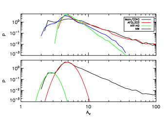
Figure 9.— Top: Probability Density Functions (PDF) for each field in W3 without correcting for the foreground/background emission. Bottom: Global PDF for the entire W3 GMC with two fitted lognormal functions (green and red), and a power-law tail (blue). The uncorrected PDF is characterized by a double-peak profile.

Visual inspection of the column density maps revealed that the material traced by this secondary peak was associated with diffuse material external to the W3 GMC, i.e., below average internal environmental conditions in the GMC. Indeed, as shown in the text, removal of foreground/background material effectively eliminated most of the component associated with this first peak. Only a “remnant” of a peak is still observed for the W3 Main/(OH) field in Figure 9. This leftover feature is expected as our correction did not remove contributions from the interstellar medium (ISM) local to W3 (i.e., in the velocity range of W3 itself), adding to the shift of pixels towards lower extinction values when removing the ISM contribution. This example emphasizes the need for a careful selection of the area chosen for PDF analysis. Note that this type of “double-peaked” PDF does not correspond to the ones observed in the vicinity of H II regions (Schneider et al., 2012; Tremblin et al., 2014) where the expansion of ionized gas into the molecular cloud leads to a compressed layer of gas that shows up in the column density PDF as a second peak at higher column densities.

While the effects on the PDF depend on the amount of ISM correction required for a particular field, this correction is most important and dominant at relatively low extinctions. This higher degree of uncertainty should be taken into consideration when analyzing those regions/structures with $A_{\mathrm{V}}<10$ mag. Correcting for line-of-sight material broadens and shifts the main peak of the PDFs to lower extinctions, which change from $A_{\mathrm{V}}\sim 5$ mag to $A_{\mathrm{V}}\sim 3$ mag. The first break of the PDFs is observed to shift by $A_{\mathrm{V}}\sim 1$ mag, while changes to the histograms are essentially negligible (within binning accuracy of $0.5$ mag) for $A_{\mathrm{V}}\gtrsim 30$ mag.

The amount of correction needed will ultimately vary from cloud to cloud, and even region to region. The KR 140 field, for instance, suffers from the greatest uncertainties due to it being severely affected by considerable foreground material traced by CO, therefore requiring the largest correction of all fields in W3. Indeed, this field has the largest difference in total mass before and after ISM correction (a factor of 1.6 more mass in the uncorrected maps), and shows the largest discrepancies in terms of mass above $A_{\mathrm{V}}$(SF) ($\sim 3.5$ less mass in the corrected mass for the same extinction level; Table 2). The mean difference in mass above $A_{\mathrm{V}}$(SF) between corrected and uncorrected maps for the other fields is $\sim 20$ % of the total corrected mass in each field, with the uncorrected maps always having more material than the corrected ones for any given extinction limit. This situation provides an upper limit to the mass uncertainties, as some correction for line-of-sight-material is required. Moreover, when dealing with uncorrected images, the $A_{\mathrm{V}}$(SF) for each field should be higher than those derived from the ISM-corrected PDFs. Therefore, the difference between the total mass above $A_{\mathrm{V}}$(SF) for the uncorrected and corrected maps should be smaller than those quoted here. None of these uncertainties affect the conclusions from this study.

Appendix B Converting between CMDs and PDFs

Similar to the interpretation of the break from the lognormal distribution in the PDF (Section 4.1), it has been suggested that the point at which a break occurs in the CMD at low extinction separates the turbulent environment from the gravity dominated structures ($A_{\mathrm{V}}$(SF); Froebrich & Rowles, 2010).

Linear regimes in the CMDs were first selected as those regions with slow varying gradient change, relative to those with significantly rapid change that should characterize a potential transition or break. These linear regimes were fitted in the CMDs with a line function and a $\chi^{2}$ minimization routine. The final slopes and intercepts in Table 1 are those of the linear fits that best represent the data neighbouring the regions of maximum gradient change (closest to the breaks) as well as the overall shape of the CMD. By fitting the separate extinction regimes of the $\log$ of the CMDs with straight lines (e.g., Figures 5 and 6), these breaks can be identified as the points where linear fits of adjacent regions intersect. The sharper the transition between two regimes (with only a small region of curvature joining adjacent linear-like regimes) the better the constraint on the value of the break.

Considering the complexity of the PDF tails and the difficulty of fitting them assuming the typical power-law function, in this work we explored using the CMDs and the straightforward linear fitting method described above as the primary approach for locating the breaks. Because a CMD is just a cumulative form derived from a PDF, however, any physical break should be recognizable when using either of the two methods.

To check for consistency of breaks derived from the CMDs with features observed in the PDFs, we transferred our best linear fits of the CMDs ($Y\equiv\log M$ vs. $A_{\mathrm{V}}$) to the form of the PDFs (linear binning). This transfer was done numerically. Quite generally, the fraction of material (expressed here as a probability $p$) in a given region with extinction between $A_{\mathrm{V},1}$ and $A_{\mathrm{V},2}$ (average $A_{\mathrm{V}}$) is

$$p(A_{\mathrm{V}})=\frac{10^{Y_{2}}-10^{Y_{1}}}{f\thinspace n_{p}\thinspace A_{V}\thinspace\mathrm{Bin}}\thinspace,$$ (B1)

where $Y_{i}$ is the plotted $\log$ of the CMD at $A_{\mathrm{V}_{i}}$, $f$ is the constant relating mass per pixel to extinction (Section 2), $n_{p}$ is the number of valid pixels in the field, and “Bin” is the linear bin size in $A_{\mathrm{V}}$ used in the PDF. This can then be transformed to the logarithmized PDFs as displayed above. For each line fitted to the CMDs the corresponding colored curves are plotted in the left panels of Figures 5 and 6.

For the specific case in Table 1 and Figures 5 and 6, where $\log M=a\thinspace A_{\mathrm{V}}+\log M(0)$ or

$$\ln M=s\thinspace A_{\mathrm{V}}+\ln M(0)\thinspace,$$ (B2)

using $c=\ln 10$ and $s=-ca$, the underlying PDF generating function is

$$p(A_{\mathrm{V}})=\frac{M(0)\thinspace s}{A_{\mathrm{V}}\thinspace fn_{p}}\exp(-sA_{\mathrm{V}})\thinspace.$$ (B3)

When cast in the format needed for the logarithmized dependent and independent variables used in Figures 5 or 6, left, the curve has the form $\log P_{\ell 10}(\log A_{\mathrm{V}})=[\thinspace\log M(0)+\log(-c^{2}a)-\log(fn_{p})\thinspace]+a\thinspace 10^{\log A_{\mathrm{V}}}$.

References

- Alves et al. (2007) Alves, J., Lombardi, M., & Lada, C. J. 2007, A&A, 462, L17
- André et al. (2011) André, P., Men’shchikov, A., Könyves, V., & Arzoumanian, D. 2011, in IAU Symposium, Vol. 270, Computational Star Formation, ed. J. Alves, B. G. Elmegreen, J. M. Girart, & V. Trimble, 255–262
- André et al. (2010) André, P., Men’shchikov, A., Bontemps, S., et al. 2010, A&A, 518, L102
- Ballesteros-Paredes et al. (2011) Ballesteros-Paredes, J., Vázquez-Semadeni, E., Gazol, A., et al. 2011, MNRAS, 416, 1436
- Bohlin et al. (1978) Bohlin, R. C., Savage, B. D., & Drake, J. F. 1978, ApJ, 224, 132
- Boneberg et al. (2015) Boneberg, D. M., Dale, J. E., Girichidis, P., & Ercolano, B. 2015, MNRAS, 447, 1341
- Carpenter et al. (2000) Carpenter, J. M., Heyer, M. H., & Snell, R. L. 2000, ApJS, 130, 381
- Dale & Bonnell (2011) Dale, J. E., & Bonnell, I. 2011, MNRAS, 414, 321
- Dale et al. (2007) Dale, J. E., Clark, P. C., & Bonnell, I. A. 2007, MNRAS, 377, 535
- Dale et al. (2015) Dale, J. E., Ercolano, B., & Bonnell, I. A. 2015, ArXiv e-prints, arXiv:1504.05896
- Dale et al. (2013) Dale, J. E., Ngoumou, J., Ercolano, B., & Bonnell, I. A. 2013, MNRAS, 436, 3430
- Evans et al. (2009) Evans, N. J., Dunham, M. M., Jørgensen, J. K., et al. 2009, ApJS, 181, 321
- Federrath & Klessen (2013) Federrath, C., & Klessen, R. S. 2013, ApJ, 763, 51
- Federrath et al. (2014) Federrath, C., Schrön, M., Banerjee, R., & Klessen, R. S. 2014, ApJ, 790, 128
- Feigelson & Townsley (2008) Feigelson, E. D., & Townsley, L. K. 2008, ApJ, 673, 354
- Fischera (2014) Fischera, J. 2014, A&A, 565, A24
- Froebrich & Rowles (2010) Froebrich, D., & Rowles, J. 2010, MNRAS, 406, 1350
- Hachisuka et al. (2004) Hachisuka, K., Brunthaler, A., Hagiwara, Y., et al. 2004, in European VLBI Network on New Developments in VLBI Science and Technology, ed. R. Bachiller, F. Colomer, J.-F. Desmurs, & P. de Vicente, 317
- Hill et al. (2011) Hill, T., Motte, F., Didelon, P., et al. 2011, A&A, 533, A94
- Hill et al. (2012) —. 2012, A&A, 542, A114
- Hughes & Viner (1982) Hughes, V. A., & Viner, M. R. 1982, AJ, 87, 685
- Kainulainen et al. (2009) Kainulainen, J., Beuther, H., Henning, T., & Plume, R. 2009, A&A, 508, L35
- Klessen (2000) Klessen, R. S. 2000, ApJ, 535, 869
- Klessen et al. (2004) Klessen, R. S., Ballesteros-Paredes, J., Li, Y., & Mac Low, M.-M. 2004, in Astronomical Society of the Pacific Conference Series, Vol. 322, The Formation and Evolution of Massive Young Star Clusters, ed. H. J. G. L. M. Lamers, L. J. Smith, & A. Nota, 299
- Koenig et al. (2012) Koenig, X. P., Leisawitz, D. T., Benford, D. J., et al. 2012, ApJ, 744, 130
- Krumholz & McKee (2008) Krumholz, M. R., & McKee, C. F. 2008, Nature, 451, 1082
- Krumholz et al. (2014) Krumholz, M. R., Bate, M. R., Arce, H. G., et al. 2014, Protostars and Planets VI, 243
- Markwardt (2009) Markwardt, C. B. 2009, in Astronomical Society of the Pacific Conference Series, Vol. 411, Astronomical Society of the Pacific Conference Series, ed. D. A. Bohlender, D. Durand, & P. Dowler, 251
- Megeath et al. (2008) Megeath, S. T., Townsley, L. K., Oey, M. S., & Tieftrunk, A. R. 2008, Low and High Mass Star Formation in the W3, W4, and W5 Regions, ed. Reipurth, B., 264
- Moore et al. (2007) Moore, T. J. T., Bretherton, D. E., Fujiyoshi, T., et al. 2007, MNRAS, 379, 663
- Motte et al. (2010) Motte, F., Zavagno, A., Bontemps, S., et al. 2010, A&A, 518, L77
- Navarete et al. (2011) Navarete, F., Figueredo, E., Damineli, A., et al. 2011, AJ, 142, 67
- Ngoumou et al. (2015) Ngoumou, J., Hubber, D., Dale, J. E., & Burkert, A. 2015, ApJ, 798, 32
- Oey et al. (2005) Oey, M. S., Watson, A. M., Kern, K., & Walth, G. L. 2005, AJ, 129, 393
- Pilbratt et al. (2010) Pilbratt, G. L., Riedinger, J. R., Passvogel, T., et al. 2010, A&A, 518, L1
- Planck Collaboration XI (2014) Planck Collaboration XI. 2014, A&A, 571, A11
- Polychroni et al. (2012) Polychroni, D., Moore, T. J. T., & Allsopp, J. 2012, MNRAS, 422, 2992
- Rivera-Ingraham et al. (2011) Rivera-Ingraham, A., Martin, P. G., Polychroni, D., & Moore, T. J. T. 2011, ApJ, 743, 39
- Rivera-Ingraham et al. (2013) Rivera-Ingraham, A., Martin, P. G., Polychroni, D., et al. 2013, ApJ, 766, 85
- Rivera-Ingraham (2012) Rivera-Ingraham, A. D. 2012, PhD thesis, University of Toronto
- Roccatagliata et al. (2011) Roccatagliata, V., Bouwman, J., Henning, T., et al. 2011, ApJ, 733, 113
- Roy et al. (2013) Roy, A., Martin, P. G., Polychroni, D., et al. 2013, ApJ, 763, 55
- Russeil et al. (2013) Russeil, D., Schneider, N., Anderson, L. D., et al. 2013, A&A, 554, A42
- Sakai et al. (2007) Sakai, T., Oka, T., & Yamamoto, S. 2007, ApJ, 662, 1043
- Schneider et al. (2012) Schneider, N., Csengeri, T., Hennemann, M., et al. 2012, A&A, 540, L11
- Schneider et al. (2013) Schneider, N., André, P., Könyves, V., et al. 2013, ApJ, 766, L17
- Straižys & Kazlauskas (2010) Straižys, V., & Kazlauskas, A. 2010, Baltic Astronomy, 19, 1
- Taylor et al. (2003) Taylor, A. R., Gibson, S. J., Peracaula, M., et al. 2003, AJ, 125, 3145
- Tieftrunk et al. (1997) Tieftrunk, A. R., Gaume, R. A., Claussen, M. J., Wilson, T. L., & Johnston, K. J. 1997, A&A, 318, 931
- Tremblin et al. (2014) Tremblin, P., Schneider, N., Minier, V., et al. 2014, A&A, 564, A106
- Voroshilov et al. (1985) Voroshilov, V. I., Guseva, N. G., Kalandadze, N. B., et al. 1985, Catalog of BV magnitudes and spectral classes of 6000 stars, ed. Voroshilov, V. I., Guseva, N. G., Kalandadze, N. B., Kolesnik, L. N., Kuznetsov, V. I., Metreveli, M. D., & Shapovalov, A. N.
- Walch et al. (2013) Walch, S., Whitworth, A. P., Bisbas, T. G., Wünsch, R., & Hubber, D. A. 2013, MNRAS, 435, 917
- Whitworth et al. (1994) Whitworth, A. P., Bhattal, A. S., Chapman, S. J., Disney, M. J., & Turner, J. A. 1994, MNRAS, 268, 291
- Xu et al. (2013) Xu, J.-L., Wang, J.-J., & Liu, X.-L. 2013, A&A, 559, A113
- Xu et al. (2006) Xu, Y., Reid, M. J., Zheng, X. W., & Menten, K. M. 2006, Science, 311, 54