Photometric Metallicity Calibration with SDSS and SCUSS and its Application to distant stars in the South Galactic Cap

Abstract

Based on SDSS g, r and SCUSS (South Galactic Cap of u-band Sky Survey) $u$ photometry, we develop a photometric calibration for estimating the stellar metallicity from $u-g$ and $g-r$ colors by using the SDSS spectra of 32,542 F- and G-type main sequence stars, which cover almost $3700$ deg² in the south Galactic cap. The rms scatter of the photometric metallicity residuals relative to spectrum-based metallicity is $0.14$ dex when $g-r<0.4$, and $0.16$ dex when $g-r>0.4$. Due to the deeper and more accurate magnitude of SCUSS $u$ band, the estimate can be used up to the faint magnitude of $g=21$. This application range of photometric metallicity calibration is wide enough so that it can be used to study metallicity distribution of distant stars. In this study, we select the Sagittarius (Sgr) stream and its neighboring field halo stars in south Galactic cap to study their metallicity distribution. We find that the Sgr stream at the cylindrical Galactocentric coordinate of $R\sim 19$ kpc, $\left|z\right|\sim 14$ kpc exhibits a relative rich metallicity distribution, and the neighboring field halo stars in our studied fields can be modeled by two-Gaussian model, with peaks respectively at [Fe/H]$=-1.9$ and [Fe/H]$=-1.5$.

1 Introduction

In the standard hierarchical model of galaxy formation, galaxies like the Milky Way were constructed by repeated aggregation with dwarf galaxies and this merging process left behind many streams, satellites, and substructures in the Galactic halo (Searle & Zinn., 1978). The Two Micro All-Sky Survey (2MASS) and Sloan Digital Sky Survey (SDSS; Abazajian et al., 2009) provided astronomers a great opportunity to detect the substructures in the spheroid of the Milky Way photometrically and spectroscopically (Yanny et al., 2000; Newberg et al., 2002; Majewski et al., 2003; Ivezić et al., 2000; Yanny et al., 2003; Newberg et al., 2007; Grillmair & Dionatos et al., 2006; Willett et al., 2009; Belokurov et al., 2006a, b; Grillmair et al., 2006a, b; Belokurov et al., 2007; Grillmair, 2009). Among all the substructures, the most prominent is the tidal stream from the disrupting Sgr dwarf spheroid galaxy which was discovered by Ibata et al. (1994). Others include the Monoceros Ring (Yanny et al., 2003), the Hercules-Aquila Cloud (Belokurov et al., 2007) and overdensity in the direction of Virgo (Jurić et al., 2008), and so on.

The Sloan Extension for Galactic Understanding and Exploration (SEGUE) Survey obtained about 240,000 low resolution spectra of faint stars ($14.0<g<20.0$) of a wide variety of spectral types. The limited number of spectra is far from enough to study the metallicity distribution of a vast area of the Galaxy. The advantage of using the photometric metallicity is that the metallicity of many more stars can be obtained. Ivezić et al. (2008) derived a photometric metallicity relations in $u-g$ vs. $g-r$ plane by using F-and G-type main sequence stars, and studied the metallicity distribution of the Galaxy. However, the SDSS $u$ band photometry is limited to $u\sim 22$. Additionally, due to the relatively large error of SDSS $u$ band magnitude near the faint end, the application of the photometric metallicity estimates is greatly restricted in the range of $g<19.5$, an insufficient depth to explore distant substructures. Based on a calibration of less metallicity-sensitive color indexes in the $gri$ passbands with well-determined spectroscopic metal abundances, An et al. (2009) determined the metal abundance estimates for main-sequence stars in the Virgo Overdensity. Karaali et al. (2011) used the UBV photometry to derive the improved metallicity Calibration. In this study, we will use a deep photometric survey, South Galactic Cap of $u$-band Sky Survey (SCUSS), to give a photometric calibration for estimating the stellar metallicity. The SCUSS $u$ is 1.5 mag deeper than SDSS $u$. This deep SCUSS $u$-band data can probe a much larger volume of the halo that enable us to study the MDF of distant stream.

Over the past decades, considerable efforts have also been made to gain information about the metallicity distribution of the Sgr system (Smecker-Hane et al., 2002; Bonifacio et al., 2004; Monaco et al., 2003, 2005; Vivas et al., 2005; Chou et al., 2007). Many works on metallicity of Sgr stream are based either on high-resolution spectra of a small amount of stars or on low-resolution spectra of giant stars. Based on high-resolution spectra, Bellazzini et al. (2008) selected 321 RGB stars in the Sgr nucleus and give the mean metallicity of $-0.45$ dex from the infrared CaII triplet. Yanny et al. (2009) traced the Sgr stream with 33 red K/M giant stars from SDSS low-resolution spectra and found an mean metallicity in the range of $-0.8\pm 0.2$. Using CFHTLS data, Sesar et al. (2011) detected the Sgr stream in $l=173^{\circ}$ and $b=-62^{\circ}$ as an overdensity of [Fe/H]$\sim-1.5$ at $R_{gal}\sim 32$ kpc. Shi et al. (2012) selected 556 red horizontal branch stars along the Sgr streams from SDSS DR7 spectroscopic data, and found that the Sgr stars have two peaks in the metallicity distribution while the Galactic stars have a more prominent metal-poor peak. Up to now, the Sgr MDF remain controversial due to different studies. In this study, we attempt to estimate the photometric MDF of the Sgr stream in south Galactic cap, which is as an application of the SCUSS photometric metallicity calibration. Additionally, we also evaluate the MDF of the field halo stars which are in the vicinity of the Sgr stream.

The outlines of this paper are as follows. We take a brief overview of the SDSS and SCUSS in Section 2, and give the SCUSS photometric metallicity calibration in Section 3. Section 4 presents the overdensities in the south Galactic cap. In Section 5, we discuss the photometric metallicity distribution of the Sgr stream in certain region and its neighboring field. A summary is given in Section 6.

2 An overview of the SDSS and SCUSS

The SDSS is a digital multi-filter imaging and spectroscopic redshift survey using a dedicated 2.5 m telescope (Gunn et al., 2006). It covers more than one-quarter of the celestial sphere in the north Galactic cap, as well as a small ($\sim 300$ deg²) but much deeper survey in the south Galactic hemisphere. It uses five bands ($u$, $g$, $r$, $i$, and $z$) to simultaneously measure brightness of stars with the effective wavelength 3562, 4686, 6165, 7481, and 8931 Å  respectively. Its magnitude limits (95% completeness for point source) are 22.0, 22.2, 22.2, 21.3, and 20.5 for $u$, $g$, $r$, $i$, and $z$ respectively (Abazajian et al., 2004). The relative photometric calibration accuracy for $u$, $g$, $r$, $i$, and $z$ are 2%, 1%, 1%, 1% and 1% respectively (Padmanabhan et al., 2008). The other technical details about SDSS can be found on the SDSS website http://www.sdss3.org/, which also provide interface for the public data access.

The South Galactic Cap u-band Sky Survey (SCUSS) is an international cooperative project, which is undertaken by National Astronomical Observatories, Chinese Academy of Sciences and Steward Observatory, University of Arizona, USA. It is an $u$ band (3538 Å) imaging survey program with the 90 inch (2.3 m) Bok telescope located on Kitt Peak, near Tucson, AZ. It will also provide part of the essential input data to the Large Sky Area Multi-Object Fiber Spectroscopic Telescope (LAMOST) project (Zhao et al., 2006). The $u$ band filter used in SCUSS project is similar to SDSS $u$ band filter but a little bluer. Fig. 1 displays both SCUSS and SDSS system response functions. The effective wavelength of the SCUSS $u$ band is about 3538 Å, and the full width half maximum (FWHM) is about 520 Å. By testing the data obtained from previous camera and new 90 Prime camera of BOK telescope, the limiting magnitude of SCUSS $u$ band may be 1.5 mag deeper than that of SDSS $u$ (Jia et al., 2014; Peng et al., 2015). The SCUSS project began its observation in 2010 and ended in 2013. Finally, 3700 square degrees field in the south Galactic cap ($30^{\circ}<l<210^{\circ},~{}-80^{\circ}<b<-20^{\circ}$) were surveyed. The SCUSS can be used to study Star formation rate, Galactic interstellar extinction, Galaxy morphology, the Galaxy structure, Quasi-Stellar Object, Variable star and Cosmology. In Table 1, we list the parameters of SCUSS and SDSS filters. Column (1) represents the ID of SCUSS and SDSS filters. and columns (2) and (3) represent effective wavelengths and full width at half maximum (FWHM) of six filters, respectively (Jia et al., 2014). The detailed information and data reduction about SCUSS can be found in Zhou et al. (2015) and Zou et al. (2015a).

Table 1: Parameters of SCUSS and SDSS filters. Column (1) represents the ID of SCUSS and SDSS filters, and columns (2) and (3) represent effective wavelengths and full width at half maximum (FWHM) of six filters, respectively.

Filter	Wavelength	FWHM
	(Å)	(Å)
$u$ (SCUSS)	3538	520
$u$ (SDSS)	3562	575
$g$	4686	1390
$r$	6165	1370
$i$	7481	1530
$z$	8931	950

Figure 1: Response curves of both the SCUSS $u$ and the SDSS $u$ filters. Both curves include the atmospheric extinction at the airmass of 1.3 and normalized to their maxima. The SCUSS $u$ band filter has about 24 Å blue shift and is slightly narrower than SDSS $u$ band filter.

The relation between SDSS $u$ and SCUSS $u$ can be expressed by following polynomial transformation:

$$u_{\rm SCUSS}= u_{\rm SDSS}-0.1373(u_{\rm SDSS}-g)$$

$$+0.0438(u_{\rm SDSS}-g)^{2}+0.1036$$

where $0.8<u_{\rm SDSS}-g<2.8$. The corresponding error of the transformed SCUSS $u$ magnitude is estimated by error transfer. The transformation is derived by point sources with SCUSS and SDSS photometric errors less than 0.05 mag. It is applied to point sources, and maximum systematic difference between SCUSS and SDSS is about 0.036 mag (Zou et al., 2015b).

3 Photometric metallicity calibration

In the SCUSS database, each star has a $u$ band magnitude and its corresponding error, as well as the position ($ra~{}\&~{}dec$). We can identify the same star from the SDSS by matching the position. Each star also has its unique ID, $u,g,r,i,z$ band magnitude, photometric error and extinction which are derived from SDSS database (hereafter, when not specified, we use $u$ to only denote the magnitude from SCUSS). Throughout this paper we use the extinction values from Schlegel et al. (1998) which are provided in the SDSS database.

The stellar parameters, such as effective temperature, surface gravity, and metallicity (parameterized as [Fe/H]) are derived with sufficient accuracy from SDSS stellar spectra. Since the number of stars from spectroscopic survey is far smaller than those from photometric survey, it is unable to get a whole picture of stellar metallicity distribution from vast area. Considering that the exhaustion of metals in a stellar atmosphere has detectable effect on the emergent flux (Schwarzschild et al., 1955), in particular in the blue region where the density of metallicity absorption is highest, the combination of spectroscopic data and photometric data can derive the estimates of [Fe/H] (Allende Prieto et al., 2006, 2008; Lee et al., 2008a, b). Ivezić et al. (2008) derived a metallicity estimator using third-order polynomials. We adopt the procedure suggested in Ivezić et al. (2008) to derive a metallicity estimator only with the exception that we use SCUSS $u$ magnitude rather than SDSS $u$. At first, we get the adopted stellar parameters (estimated through the SEGUE Stellar Parameter Pipeline [SSPP] Beers et al. (2006) of the stellar spectroscopic survey from sppParams table in SDSS website (http://www.sdss3.org/), and then find the same stars from SCUSS database by matching the shared ID number of stars. After excluding the repeated stars surveyed in different plates, we eventually obtain a database of 74,133 stars with SCUSS $u$ magnitude, SDSS $g,r,i,and~{}z$ magnitude, as well as the SEGUE stellar parameters.

In order to derive the photometric metallicity estimate, we adopt the same selection criteria used by Ivezić et al. (2008). We relist these criteria as follows:

• The interstellar extinction in the $r$ band below 0.3;

• $14<g<19.5$;

• $0.2<(g-r)<0.6$;

• $0.7<(u-g)<2.0$ and $-0.25<(g-r)-0.5(u-g)<0.05$;

• $-0.2<0.35(g-r)-(r-i)<0.10$;

• $log(g)>3$.

Through these selection criteria, we eventually get 32,542 stars to determine a photometric metallicity ([Fe/H]_phot) estimate. The median metallicity of the above selected sample stars shows a complex behavior as a function of $u-g$ and $g-r$ colors which is consistent with the result of Ivezić et al. (2008). To reliably estimate the photometric metal abundance, it is necessary that these stars are separated by $g-r=0.4$ into two regions in the $u-g$ versus $g-r$ plane to avoid relative large systematic errors. Then, we adopt third-order polynomials to fit the median metallcity with the color $u-g$ and $g-r$. The resulting estimate is as follows:

when        $y<0.4$

$$\rm[Fe/H]= 17.68-91.34x+60.55y+110.7x^{2}$$

$$-65.02xy-71.72y^{2}-41.54x^{3}$$

$$+33.42x^{2}y-3.734xy^{2}+58.92y^{3}$$

when       $y>0.4$

$$\rm[Fe/H]= 12.89-6.322x-79.79y+17.06x^{2}$$

$$-38.62xy+199.1y^{2}-18.85x^{3}$$

$$+102.8x^{2}y-212.8xy^{2}+38.17y^{3}$$

where $x=u-g$, $y=g-r$.

Using the above equations, the photometric metallicty [Fe/H]_phot is computed for each star and compared with the spectroscopic metallicity. The rms scatter of the photometric metallicity residuals relative to spectrum-based metallicity is $0.14$ dex when $g-r<0.4$, and $0.16$ dex when $g-r>0.4$. So the photometric estimates are relatively reliable to provide a good estimation for the large number of photometric surveyed stars. The random metallicity error mainly comes from the photometric error of $u$ band magnitude. As shown in Fig. 2, the average error of SCUSS $u$ magnitude in most observation field (here, about 50,000 stars as an example) is small than SDSS $u$ on the whole. From this figure we see that SDSS $u$ error of 0.09 corresponds to $g$ magnitude of 19.5. However, the same error of SCUSS $u$ corresponds to deeper $g$ magnitude of 20.5. The $g$ magnitude of 21 corresponds to SCUSS $u$ error of 0.13. Due to its relative deep magnitude and high accuracy from SCUSS data, we expect wide range of application of the photometric estimate. We obtain a star sample from the SCUSS database under the criteria mentioned above except $log(g)>3$, and compute the rms statistical scatter of [Fe/H]_phot introduced by the $u$ band photometric error. The rms statistical scatter of metallicity increases with $g$ magnitude from $0.014$ dex for $g<17$ to $0.070$ dex at $g=18.5$, $0.379$ dex at $g=20.5$, $0.445$ dex at $g=21$ and $0.750$ dex at $g=21.3$. So we limit the application of photometric estimates in the range of $g<21$, where the maximum rms scatter of the metallicity is $0.445$ dex. This application of [Fe/H]_phot allows the metallicity to be determined for all SCUSS stars in these criteria range. So we can derive the [Fe/H]_phot for numerous farther stars.

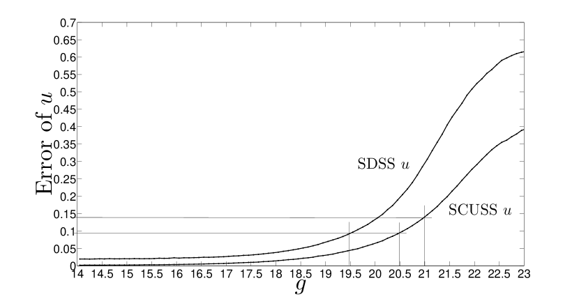
Figure 2: The average error of $u$ magnitude of 50,000 stars as a function of $g$ magnitude. The SCUSS $u$ error is smaller than SDSS $u$ error on the whole. From this figure we see that SDSS $u$ error of 0.09 corresponds to $g$ magnitude of 19.5. However the same error of SCUSS $u$ corresponds to deeper $g$ magnitude of 20.5. The $g$ magnitude of 21 corresponds to SCUSS $u$ error of 0.13, which may introduce the rms scatter of photometric metallicity estimate up to $0.445$ dex.

To show how well the present SCUSS photometric metallicity predictions agree with SDSS photometric metallicity predictions, here as an example, we randomly select a few main sequence stars, which are bright enough (with $g<19$) to be well-detected in both SDSS $u$ and SCUSS $u$, to evaluate their metallicity, respectively from SDSS $u$ and SCUSS $u$ (see Table. 2). In Table 2, Column (1) shows the g magnitude bins, and the rest columns in each row give the mean values of information about a bunch of stars which belong to the corresponding bins. The last two columns give the mean metallicity values estimated respectively from SDSS $u$ and SCUSS $u$. From the table we can easily find that SCUSS $u$ photometric metallicity estimate is almost consistent with the SDSS $u$ photometric metallicity estimate. Nevertheless, despite agreements in both photometric metallicity estimates at bright magnitude, there still exists mismatches for part stars especially at relatively faint magnitude.

Table 2: Comparison of the photometric metallicity estimate from SDSS $u$ and SCUSS $u$, for bright stars ($g<19$). Column (1) shows the g magnitude bins, and the rest columns in each row give the mean values of information about a bunch of stars which belong to the corresponding bins. The last two columns give the mean metallicity values estimated respectively from SDSS $u$ and SCUSS $u$.

Interval of $g$ magnitude	SDSS $u_{mean}$	SCUSS $u_{mean}$	$g_{mean}$	$r_{mean}$	[Fe/H]mean	[Fe/H]mean
					from SDSS $u$	from SCUSS $u$
16.0 $\sim$ 16.5	17.63	17.79	16.44	15.94	-0.67	-0.85
16.5 $\sim$ 17.0	18.10	18.10	16.76	16.27	-0.90	-0.93
17.0 $\sim$ 17.5	18.55	18.55	17.26	16.78	-0.94	-0.94
17.5 $\sim$ 18.0	19.04	19.04	17.75	17.27	-1.02	-1.01
18.0 $\sim$ 18.5	19.56	19.55	18.26	17.76	-1.16	-1.16
18.5 $\sim$ 19.0	20.05	20.05	18.76	18.27	-1.39	-1.35

4 The overdensities in the south Galactic cap

The SCUSS covers the south Galactic cap ($30^{\circ}<l<210^{\circ},~{}-80^{\circ}<b<-20^{\circ}$) and it stretches a wide range along the celestial equator. As shown in Fig. 3, we select the F/G stars ($0.2<g-r<0.4$) as sample stars to trace the overdensities. In contrast, we plot two two-color diagrams $u-g$ vs. $g-r$, the upper figure is plotted using SDSS $u$ with selection criteria $u<23.5,g<22.4,r<22.1,r>15$, while the bottom one using SCUSS $u$ with the same criteria. We can also clearly find that the stars in the upper diagram which uses SDSS $u$ are more scattered, especially in the blue end. It provides an illustration of reduced statistical errors of SCUSS $u$. We also use the condition $u-g>0.6$ to remove the quasars. In addition, since SCUSS $u$ has the limit magnitude of $23.5$, whereas SDSS $u$ has the limit magnitude of $22.1$, we expect to pick out more sample stars from SCUSS database. We have selected F/G stars from 50,000 stars in SCUSS database and find that there are 4,566 F/G stars when using SCUSS $u$ with $u<23.5$, but only 3,572 stars when using SDSS $u$ with $u<22.1$.

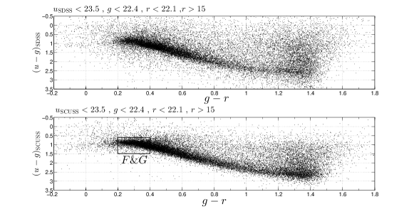
Figure 3: $u-g$ vs. $g-r$ two-color diagram of 50,000 stars randomly selected from the SCUSS database. The upper figure is plotted using SDSS $u$ with selection criteria $u<23.5,g<22.4,r<22.1,r>15$, while the bottom one using SCUSS $u$ with the same criteria. Here, we choose F/G stars as tracers from the color box $u-g>0.6,~{}0.2<g-r<0.4$ as indicated by the rectangular box in the bottom figure.

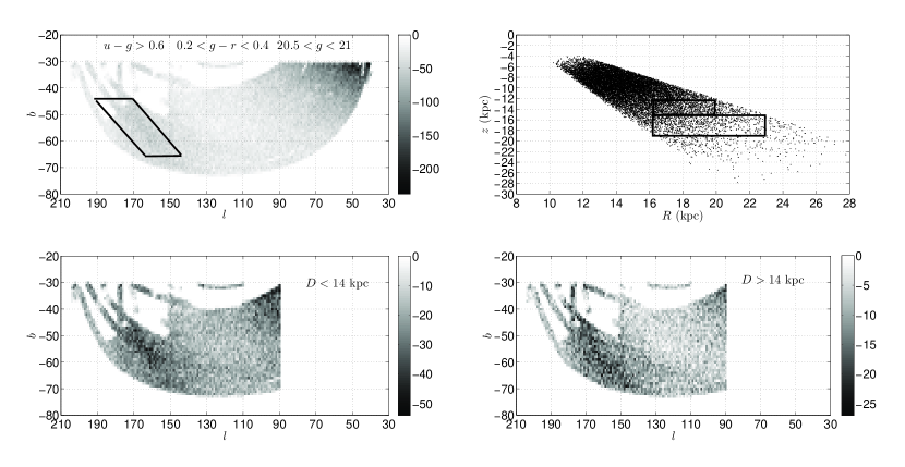
Figure 4: Top left panel: Spatial distribution of the F/G stars with $20.5<g<21$. Top right panel: Distribution of the F/G main sequence stars with $20.5<g<21$ in the Sgr stream area (surrounded by parallelogram) in cylindrical galactocentric coordinate system. Bottom two panel: Spatial distribution of F/G stars with heliocentric distance $D<14$ kpc and $D>14$ kpc, respectively. The three gray-scale bars all indicate star count density in each pixel ($1^{\circ}\times 1^{\circ}$).

After comparing with F/G stars spatially in different magnitude bin, we find that the overdensity is spatially obvious in the range of $20.5<g<21$ for the SCUSS observation, as shown in the top left panel in Fig. 4. From Fig. 4, we can see two overdensities: Sgr stream and Hercules-Aquila cloud which were discovered previously (Ibata et al., 1994; Newberg et al., 2002; Belokurov et al., 2007). But the Sgr stream in the top left panel of Fig. 4 is less distinct, we select the Sgr stream stars further by distance cut-off. It consists of the following procedures:

• Selecting main sequence stars by rejecting those objects at distances larger than $0.15$ mag from the stellar locus which is described by following Equation (Jurić et al., 2008)

  $$(g-r)_{0}= 1.39\{1-exp[-4.9(r-i)_{0}^{3}-2.45(r-i)_{0}^{2}$$

  $$-1.68(r-i)_{0}-0.05]\}$$

• Computing the heliocentric distance of each star from the following equations, the parallax relation implicitly takes metallicity effects into account. (Jurić et al., 2008)

  $$M_{r}= 4.0+11.86(r-i)_{0}-10.74(r-i)_{0}^{2}$$

  $$+5.99(r-i)_{0}^{3}-1.20(r-i)_{0}^{4}$$

  $$D=10^{(r-M_{r})/5+1}$$

• Transforming the coordinate ($l,~{}b,~{}D$) into the right-handed Cartesian galactocentric coordinate ($x,~{}y,~{}z$) (Jurić et al., 2008)

  $$x=R_{\circleddot}-D\cos{(l)}\cos{(b})$$

  $$y=-D\sin{(l)}\cos{(b)}$$

  $$z=D\sin{(b)}$$

• Transforming the coordinate ($x,~{}y,~{}z$) into the cylindrical galactocentric coordinate ($R,~{}\phi,~{}z$) (Bond et al., 2010)

  $$R=\sqrt{x^{2}+y^{2}}$$

  $$\phi=\arctan{(y/x)}$$

  $$z=D\sin{b}$$

Through the above procedures, the F/G main sequence stars with $20.5<g<21$ in the Sgr stream area are picked out, which is surrounded by parallelogram in top left panel of Fig.4. At the same time, we give the spatial distribution of these sample stars in cylindrical coordinate system (top right panel of Fig.4). These stars are mainly in the eighth octant with $-22.5^{\circ}<\phi<0^{\circ}$. In order to enhance the contrast of the Sgr stream, we remove the overdensity of Hercules-Aquila cloud and divide the stars into two groups by the heliocentric distance of $D=14$ kpc. Here, we also plot the spatial distribution of stars in ($l,~{}b$) panel (bottom two panels in Fig. 4). We find that the Sgr stream stars are obvious when $D>14$ kpc. In the following study of the MDF in the Sgr stream, we mainly select those sample stars in the range of $D>14$ kpc which is shown by the two rectangles in the top right panel of Fig. 4.

5 Photometric metallicity estimation of distant stars in south Galactic cap

Since the photometric metallicity estimate we have derived in Section 3 can also be used up to the faint magnitude of $g=21$. We may use the photometric metallicity calibration to analyze the metallicity distribution of the sample stars which contain large number of Sgr steam stars. As discussed above, we have selected the sample stars via cut-off on color index $g-r$ and distance. The F/G main sequence stars with $g<21$ in the space volume ($16$ kpc $<R<20$ kpc, $-22.5^{\circ}<\phi<0^{\circ}$, $12$ kpc $<\left|z\right|<15$ kpc) and ($16$ kpc $<R<23$ kpc, $-22.5^{\circ}<\phi<0^{\circ}$, $15$ kpc $<\left|z\right|<19$ kpc) are chosen to evaluate the MDF, as illustrated in the top two panels of Fig. 5. The top two histograms in Fig. 5 correspond to the Sgr stream region. In order to have contrasts, the stars in other space volume with angle bin $\Delta\phi=22.5^{\circ},~{}45^{\circ}$ are also selected to evaluate the metallicity distribution, as illustrated in the middle and bottom panels of Fig. 5, which correspond to the vicinities of the Sgr stream region. It is clear that the Sgr stream has a wide metallicity distribution, and has much more stars from [Fe/H]$\sim-1.5$ to [Fe/H]$\sim-0.5$.

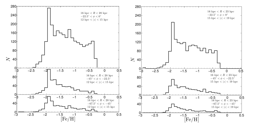
Figure 5: The metallicity distribution of the F/G ($0.2<g-r<0.4$) main sequence stars with $g<21$ in different space volume. The top two histograms correspond to the Sgr stream region. The middle and the bottom histograms correspond to the vicinities of the Sgr stream region.

Because the neighboring regions selected have the same volume as Sgr stream region, the rough way for evaluating the MDF of the Sgr stream in the selected region is to subtract the MDF of halo stars from the MDF of the mixed population in the equal volume space. As shown in Fig. 6, we subtracted the MDF of halo (bottom left panel of Fig. 5) from the mixed population (top left panel of Fig.5). The derived MDF can be assumed to be contributed mainly from the Sgr stream of the selected region. We find that the Sgr stream exhibit a relatively rich metallicity distribution. To further get the real characteristics of the MDF in the Sgr stream and halo stars, we adopted the mixed model to fit the photometric metallicity distribution. We fitted the left half MDFs in Fig. 5. We find that three-Gaussian model is appropriate for the MDF of mixed population (Sgr stream and halo stars), and two-Gaussian model for MDF of neighbouring stars (mainly the halo stars), as shown by Fig. 7. The two-Gaussian of the MDF of halo stars are with peaks at [Fe/H]$=-1.5$ and [Fe/H]$=-1.9$ respectively. This profile of the MDF of the halo stars can be explained by the argument by Carollo et al. (2007) that the halo comprises two broadly overlapping structural components, an inner and an outer halo. The three Gaussians of the mixed population are with peaks at [Fe/H]$=-1.9$, [Fe/H]$=-1.5$ and [Fe/H]$=-0.5$ respectively. By contrast, we can easily find that the extra stars at [Fe/H]$=-0.5$ reasonably belongs to the Sgr stream. However, the stars around [Fe/H]$=-1.5$ may be mixed population of Sgr stream and the inner halo. Similarly, the Gaussian with peak at [Fe/H]$=-1.9$ is contributed jointly by Sgr stream and outer halo. The parameters of the Gaussians for fitting are shown in Table 3.

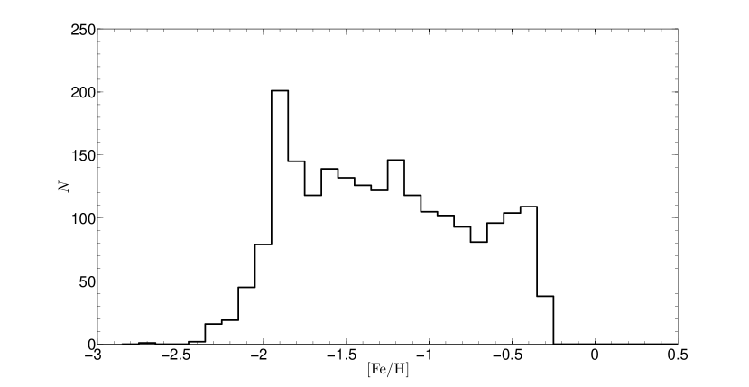
Figure 6: The derived MDF by subtraction of MDF of halo stars (bottom left panel of Fig. 5) from the Sgr region stars (top left one). It shows the wide metallicity distribution from [Fe/H]$=-0.4$ to [Fe/H]$=-2.0$.

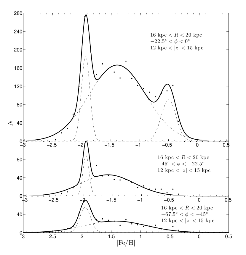
Figure 7: The Gaussian models of the left half MDFs in Fig. 5. The top MDF can be modeled by three Gaussians with peaks respectively at [Fe/H]$=-1.9$, [Fe/H]$=-1.5$ and [Fe/H]$=-0.5$. The bottom two MDFs can be modeled by two Gaussian, each with peaks at [Fe/H]$=-1.5$ and [Fe/H]$=-1.9$ respectively.

Table 3: The parameters of the Gaussians for fitting the MDFs.

$N=a1\cdot Exp{[-(\frac{x-b1}{c1})^{2}]}+a2\cdot Exp{[-(\frac{x-b2}{c2})^{2}]}+a3\cdot Exp{[-(\frac{x-b3}{c3})^{2}]}$
$a1=186.4$	$b1=-1.937$	$c1=0.1022$
$a2=166.4$	$b2=-1.397$	$c2=0.6862$
$a3=90.58$	$b3=-0.5229$	$c3=0.1777$
$N=a1\cdot Exp{[-(\frac{x-b1}{c1})^{2}]}+a2\cdot Exp{[-(\frac{x-b2}{c2})^{2}]}$
$a1=88.4$	$b1=-1.93$	$c1=0.0741$
$a2=46.41$	$b2=-1.559$	$c2=0.6376$
$N=a1\cdot Exp{[-(\frac{x-b1}{c1})^{2}]}+a2\cdot Exp{[-(\frac{x-b2}{c2})^{2}]}$
$a1=55.07$	$b1=-1.944$	$c1=0.1308$
$a2=25.15$	$b2=-1.427$	$c2=0.7478$

6 Summary

In this paper, based on SCUSS $u$ and SDSS $g,r,i,z$, we derive a photometric metallicity calibration for estimating the stellar metallicity [Fe/H]_phot by using 32,542 F- and G-type main sequence stars from SDSS spectra. The rms scatter of the photometric metallicity residuals relative to spectrum-based metallicity is $0.14$ dex when $g-r<0.4$ and $0.16$ dex when $g-r>0.4$. The rms statistical scatter of metallicity due to u-band photometric uncertainty increases with $g$ magnitude from $0.014$ dex for $g<17$ to $0.070$ dex at $g=18.5$, $0.379$ dex at $g=20.5$, $0.445$ dex at $g=21$ and $0.750$ dex at $g=21.3$. So we limit the application of photometric estimates in the range of $g<21$. This application range of [Fe/H]_phot is wide, and it allows metallicity to be determined for all SCUSS main-sequence stars in these criteria range. So we can derive the [Fe/H]_phot estimates for numerous farther stars.

As an example, we select Sgr stream and its neighboring field halo stars in south Galactic cap to study its metallicity distribution. We find that the Sgr stream around the cylindrical Galactocentric coordinate of $R\sim 19$ kpc, $\left|z\right|\sim 14$ kpc exhibit a relative rich metallicity distribution, and the MDF of the neighboring field halo stars in our studied fields can be modeled by two-Gaussian model, with peaks respectively at [Fe/H]$=-1.9$ and [Fe/H]$=-1.5$.

References

- Abazajian et al. (2009) Abazajian, K., et al. 2009, ApJS, 182, 543
- Abazajian et al. (2004) Abazajian, K. et al. 2004, AJ, 128, 502
- Allende Prieto et al. (2006) Allende Prieto, C., et al. 2006, ApJ, 636, 804
- Allende Prieto et al. (2008) Allende Prieto, C., et al. 2008, AJ, 136, 2070
- An et al. (2009) An, D., et al. 2009, ApJ, 707, L64
- Beers et al. (2006) Beers, T., C., et al. 2006, Mem. Soc. Astron. Italiana, 77, 1171
- Bellazzini et al. (2008) Bellazzini, M., Ibata, R. A., Chapman, S. C., et al. 2008, AJ, 136, 1147
- Belokurov et al. (2006a) Belokurov, V., Evans, N. W., Irwin, M. J., Hewett, P. C., & Wilkinson, M. I. 2006a, ApJ, 637, L29
- Belokurov et al. (2006b) Belokurov, V., et al. 2006b, ApJ, 642, L137
- Belokurov et al. (2007) Belokurov, V., et al. 2007, ApJ, 657, L89
- Bonifacio et al. (2004) Bonifacio, P., Sbordone, L., Marconi, G., Pasquini, L., & Hill, V. 2004, A&A, 414, 503
- Bond et al. (2010) Bond, N. A., et al. 2010, ApJ, 716, 1
- Chou et al. (2007) Chou, M. Y., Majewski, S. R., Cunhu K., Smith V. V., et al. 2007, ApJ, 670, 346
- Carollo et al. (2007) Carollo, D., et al. 2007, Nature, 450, 1020
- Grillmair & Dionatos et al. (2006) Grillmair, C. J., & Dionatos, O. 2006, ApJ, 643, L17
- Grillmair et al. (2006a) Grillmair, C. J. 2006a, ApJ 645, L37
- Grillmair et al. (2006b) Grillmair, C. J. 2006b, ApJ 651, L29
- Grillmair (2009) Grillmair, C. J. 2009, ApJ 693, 1118
- Gunn et al. (2006) Gunn, J. E., et al. 2006, AJ, 131, 2332
- Ibata et al. (1994) Ibata, R. A., Gilmore, G., & Irwin, M. J. 1994, Nature, 370, 194
- Ibata et al. (2001) Ibata, R. A., Lewis, G. F., Irwin, M., Totten, E., & Quinn, T. 2001, ApJ, 551, 294
- Ivezić et al. (2000) Ivezić, Ž., et al. 2000, AJ, 120, 963
- Ivezić et al. (2008) Ivezić, Ž., Sesar, B., et al. 2008, ApJ, 684, 287
- Jurić et al. (2008) Jurić, M., et al. 2008, ApJ, 673, 864
- Jia et al. (2014) Jia, Y.P., Du, C.H., et al. 2014, MNRAS, 441, 503
- Karaali et al. (2011) Karaali, S., Bilir, S., Ak, S., Yaz, E., et al. 2011, PASA, 28, 95
- Lee et al. (2008a) Lee, Y. S., et al. 2008a, AJ, 136, 2050
- Lee et al. (2008b) Lee, Y. S., et al. 2008b, AJ, 136, 2022
- Majewski et al. (2003) Majewski, S. R., Skrutskie, M. F., Weinberg, M. D., & Ostheimer, J. C. 2003, ApJ, 599, 1082
- Monaco et al. (2003) Monaco, L., Bellazzini, M., Ferraro, F. R., & Pancino, E. 2003, ApJ, 597, L25
- Monaco et al. (2005) Monaco, L., et al. 2005, A&A, 441, 141
- Newberg et al. (2002) Newberg, H., et al. 2002, ApJ, 569, 245
- Newberg et al. (2007) Newberg, H., Yanny, B., Cole, N., Beers, T., Re Fiorentin, P., Schneider, D., & Wilhelm, R. 2007, ApJ, 668, 221
- Padmanabhan et al. (2008) Padmanabhan N. et al. 2008, ApJ, 674, 1217
- Peng et al. (2015) Peng, X.Y., Qi, Z.Q., Wu, Z.Y., Ma, J., et al., 2015, PASP, 127, 250
- Searle & Zinn. (1978) Searle, L., & Zinn, R. 1978, ApJ, 225, 357
- Shi et al. (2012) Shi, W. B., Chen, Y. Q., et al. 2012, ApJ, 751, 130
- Schwarzschild et al. (1955) Schwarzschild, M., Searle, L., & Howard, R. 1955, ApJ, 122, 353
- Schlegel et al. (1998) Schlegel, D., J., Finkbeiner, D., P., & Davis, M. 1998, ApJ, 500, 525
- Sesar et al. (2011) Sesar, B., Jurić, M., Ivezić. 2011, ApJ, 731, 4
- Smecker-Hane et al. (2002) Smecker-Hane, T. A., & McWilliam, A. 2002, arxiv: astro-ph/0205411
- Vivas et al. (2005) Vivas, A. K., Zinn, R., & Gallart, C. 2005, AJ, 129, 189
- Willett et al. (2009) Willett, B., Newberg, H. J., Zhang, H., Yanny, B., & Beers, T. C. 2009, ApJ, 697, 207
- Yanny et al. (2000) Yanny, B., et al. 2000, ApJ, 540, 825
- Yanny et al. (2003) Yanny, B., et al. 2003, ApJ, 588, 824
- Yanny et al. (2009) Yanny, B., Newberg, H. J., Johnson, J. A., et al. 2009, ApJ, 700, 1282
- Zhao et al. (2006) Zhao, G., Chen, Y. Q., Shi, J. R., et al. 2006, Chin. J. Astro. Astrophys., 6, 265
- Zou et al. (2015b) Zou, H., Wu, X., B., et al. 2015b, PASP, 127, 94
- Zou et al. (2015a) Zou, H., et al. 2015a, AJ, submitted
- Zhou et al. (2015) Zhou, X., et al. 2015, RAA, submitted