Global existence and asymptotics for quasi-linear one-dimensional Klein-Gordon equations with mildly decaying Cauchy data

Abstract

Let u be a solution to a quasi-linear Klein-Gordon equation in one-space dimension, $\Box u+u=P(u,\partial_{t}u,\partial_{x}u;\,\partial_{t}\partial_{x}u,\partial^{2}_{x}u)$, where $P$ is a homogeneous polynomial of degree three, and with smooth Cauchy data of size $\varepsilon\rightarrow 0$. It is known that, under a suitable condition on the nonlinearity, the solution is global-in-time for compactly supported Cauchy data. We prove in this paper that the result holds even when data are not compactly supported but just decaying as $\langle x\rangle^{-1}$ at infinity, combining the method of Klainerman vector fields with a semiclassical normal forms method introduced by Delort. Moreover, we get a one term asymptotic expansion for $u$ when $t\rightarrow+\infty$.

Introduction

The goal of this paper is to prove the global existence and to study the asymptotic behaviour of the solution $u$ of the one-dimensional nonlinear Klein-Gordon equation, when initial data are small, smooth and slightly decaying at infinity. We will consider the case of a quasi-linear cubic nonlinearity, namely a homogeneous polynomial $P$ of degree 3 in $(u,\partial_{t}u,\partial_{x}u;\,\partial_{t}\partial_{x}u,\partial^{2}_{x}u)$, affine in $(\partial_{t}\partial_{x}u,\partial^{2}_{x}u)$, so the initial valued problem is written as

(1) $$\begin{cases}&\Box u+u=P(u,\partial_{t}\partial_{x}u,\partial^{2}_{x}u\,;\partial_{t}u,\partial_{x}u)\\ &u(1,x)=\varepsilon u_{0}(x)\\ &\partial_{t}u(1,x)=\varepsilon u_{1}(x)\end{cases}\qquad t\geq 1\,,x\in\mathbb{R}\,,\varepsilon\in]0,1[\,.$$

Our main concern is to obtain results for data which have only mild decay at infinity (i.e. which are $O(|x|^{-1})$, $x\rightarrow+\infty$), while most known results for quasi-linear Klein-Gordon equations in dimension 1 are proved for compactly supported data. In order to do so, we have to develop a new approach, that relies on semiclassical analysis, and that allows to obtain for Klein-Gordon equations results of global existence making use of Klainerman vector fields and usual energy estimates, instead of $L^{2}$ estimates on the hyperbolic foliation of the interior of the light cone, as done for instance in an early work of Klainerman [21] and more recently in the paper of LeFloch, Ma [24].

We recall first the state of the art of the problem. In general, the problem in dimension 1 is critical, contrary to the problem in higher dimension which is subcritical. In fact, in space dimension $d$, the best time decay one can expect for the solution is $\|u(t,\cdot)\|_{L^{\infty}}=O(t^{-\frac{d}{2}})$: therefore, in dimension 1 the decay rate is $t^{-\frac{1}{2}}$, and for a cubic nonlinearity, depending for example only on $u$, one has $\|P(u)\|_{L^{2}}\leq Ct^{-1}\|u(t,\cdot)\|_{L^{2}}$, with a time factor $t^{-1}$ just at limit of integrability. It is well known from works of Klainerman [21] and Shatah [30] that the analogous problem in space dimension $d\geq 3$ has global-in-time solutions if $\varepsilon$ is sufficiently small. In [21], Klainerman proved it for smooth, compactly supported initial data, with nonlinearities at least quadratic, using the Lorentz invariant properties of $\Box+1$ to derive uniform decay estimates and generalized energy estimates for solutions $u$ to linear inhomogeneous Klein-Gordon equations. Simultaneously, in [30] Shatah proved this result for smooth and integrable initial data, extending Poincaré’s theory of normal forms for ordinary differential equations to the case of nonlinear Klein-Gordon equations. An earlier work from Simon [31], and from Simon, Taflin in [32] for coupled Klein-Gordon equations with several masses, established the global existence for data given at $t=\infty$. In [15], Hörmander refined Klainerman’s techniques to obtain new time decay estimates of solutions to linear inhomogeneous Klein-Gordon equations and he showed that, for quadratic nonlinearities, the solution exists over $[-T_{\varepsilon},T_{\varepsilon}]$ with an existence time $T_{\varepsilon}$ such that $\lim_{\varepsilon\rightarrow 0}\varepsilon\log T_{\varepsilon}=\infty$ when $d=2$, while $\lim_{\varepsilon\rightarrow 0}\varepsilon^{2}T_{\varepsilon}=\infty$ for $d=1$. In addition, he presented two conjectures: for quadratic nonlinearities, $T_{\varepsilon}=\infty$ in two space dimensions, while for space dimension one $\liminf_{\varepsilon\rightarrow 0}\varepsilon^{2}\log T_{\varepsilon}>0$. The first conjecture has been proved by Ozawa, Tsutaya and Tsutsumi in [28] in the semi-linear case, after partial results by Georgiev, Popivanov in [9], Kosecki [23] (for nonlinearities verifying some "suitable null conditions"), and Simon, Taflin in [33]. Later, in [29] Ozawa, Tsutaya and Tsutsumi announced the extension of their proof to the quasi-linear case and studied scattering of solutions. Still in dimension 2, Delort, Fang and Xue proved in [7] the global existence of solutions for a quasi-linear system of two Klein-Gordon equations, with masses $m_{1},m_{2}$, $m_{1}\neq 2m_{2}$ and $m_{2}\neq 2m_{1}$ for small, smooth, compactly supported Cauchy data, extending the result proved by Sunagawa in [34] in the semi-linear case. Moreover, they proved that the global existence holds true also when $m_{1}=2m_{2}$ and a convenient null condition is satisfied by nonlinearities. The same result in the resonant case is also proved by Katayama, Ozawa [18], and by Kawahara, Sunagawa [19], in which the structural condition imposed on nonlinearities includes the Yukawa type interaction, which was excluded from the null condition in the sense of [7]. In this context, we cite also the work of Germain [11], and of Ionescu, Pausader [17], for a system of coupled Klein-Gordon equations with different speeds in dimension 3, with a quadratic nonlinearity, respectively in the semilinear case for the former, and in the quasi-linear one for the latter. For data small, smooth, and localized, they prove that a global solution exists and scatters.

In dimension 1, Moriyama, Tonegawa and Tsutsumi [27] have shown that the solution exists on a time interval of length longer or equal to $e^{c/\varepsilon^{2}}$, where $\varepsilon$ is the Cauchy data’s size, with a nonlinearity vanishing at least at order three at zero, or semi-linear. They also proved that the corresponding solution asymptotically approaches the free solution of the Cauchy problem for the linear Klein-Gordon equation. The fact that in general the solution does not exist globally in time was proved by Yordanov in [35], and independently by Keel and Tao [20]. However, there exist examples of nonlinearities for which the corresponding solution is global-in-time: on one hand, if $P$ depends only on $u$ and not on its derivatives; on the other hand, for seven special nonlinearities considered by Moriyama in [26]. A natural question is then posed by Hörmander, in [14, 15]: can we formulate a structure condition for the nonlinearity, analogous to the null condition introduced by Christodoulou [2] and Klainerman [22] for the wave equation, which implies global existence? In [4, 5] Delort proved that, when initial data are compactly supported, one can find a null condition, under which global existence is ensured. This condition is likely optimal, in the sense that when the structure hypothesis is violated, he constructed in [3] approximate solutions blowing up at $e^{A/\varepsilon^{2}}$, for an explicit constant $A$. This suggests that also the exact solution of the problem blows up in time at $e^{A/\varepsilon^{2}}$, but this remains still unproven.

In most of above mentioned papers dealing with the one dimensional problem, two key tools are used: normal forms methods and/or Klainerman vector fields $Z$. In particular, the latter are useful since they have good properties of commutation with the linear part of the equation, and their action on the nonlinearity $ZP(u)$ may be expressed from $u,Zu$ using Leibniz rule. This allows one to prove easily energy estimates for $Z^{k}u$ and then to deduce from them $L^{\infty}$ bounds for $u$, trough Klainerman-Sobolev type inequalities. However, in these papers the global existence is proved assuming small, compactly supported initial data. This is related to the fact that the aforementioned authors use in an essential way a change of variable in hyperbolic coordinates, that does not allow for non compactly supported Cauchy data. Our aim is to extend the result of global existence for cubic quasi-linear nonlinearities in the case of small compactly supported Cauchy data of [4, 5], to the more general framework of data with mild polynomial decay. To do that, we will combine the Klainerman vector fields’ method with the one introduced by Delort in [6].

In [6], Delort develops a semiclassical normal form method to study global existence for nonlinear hyperbolic equations with small, smooth, decaying Cauchy data, in the critical regime and when the problem does not admit Klainerman vector fields. The strategy employed is to construct, through semiclassical analysis, some pseudo-differential operators which commute with the linear part of the considered equation, and which can replace vector fields when combined with a microlocal normal form method. Our aim here is to show that one may combine these ideas together with the use of Klainerman vector fields to obtain, in one dimension, and for nonlinearities satisfying the null condition, global existence and modified scattering.

In our paper, we prove the global existence of the solution $u$ by a boostrap argument, namely by showing that we can propagate some suitable a priori estimates made on $u$. We propagate two types of estimates: some energy estimates on $u$, $Zu$, and some uniform bounds on $u$. To prove the propagation of energy estimates is the simplest task. We essentially write an energy inequality for a solution $u$ of the Klein-Gordon equation in the quasi-linear case (the main reference is the book of Hörmander [15], chapter 7), and then we use the commutation property of the Klainerman vector fields $Z$ with the linear part of the equation to derive an inequality also for $Zu$. Moreover, $Z$ acts like a derivation on the nonlinearity, so the Leibniz rule holds and we can estimate $ZP$ in term of $u,Zu$. Injecting a priori estimates in energy inequalities and choosing properly all involved constants allow us to obtain the result.

The main difficulty is to prove that the uniform estimates hold and can be propagated. Actually, as mentioned above, the one dimensional Klein-Gordon equation is critical, in the sense that the expected decay for $\|u(t,\cdot)\|^{2}_{L^{\infty}}$ is in $t^{-1}$, so is not integrable. A drawback of that is that one cannot prove energy estimates that would be uniform as time tends to infinity. Consequently, a Klainerman-Sobolev inequality, that would control $\|u(t,\cdot)\|_{L^{\infty}}$ by $t^{-1/2}$ times the $L^{2}$ norms of $u,Zu$, would not give the expected optimal $L^{\infty}$-decay of the solution, but only a bound in $t^{-\frac{1}{2}+\sigma}$ for some positive $\sigma$, which is useless to close the bootstrap argument. The idea to overcome this difficulty is, following the approach of Delort in [6], to rewrite (1) in semiclassical coordinates, for some new unknown function $v$. The goal is then to deduce from the PDE satisfied by $v$ an ODE from which one will be able to get a uniform $L^{\infty}$ bound for $v$ (which is equivalent to the optimal $t^{-1/2}$ $L^{\infty}$-decay of $u$). Let us describe our approach for a simple model of Klein-Gordon equation:

(2) $$(D_{t}-\sqrt{1+D_{x}^{2}})u=\alpha u^{3}+\beta|u|^{2}u+\gamma|u|^{2}\bar{u}+\delta\bar{u}^{3},$$

where $\alpha,\beta,\gamma,\delta$ are constants, $\beta$ being real (this last assumption reflecting the null condition on that example). Performing a semiclassical change of variables and unknowns $u(t,x)=\frac{1}{\sqrt{t}}v(t,\frac{x}{t})$, we rewrite this equation as

(3) $$[D_{t}-Op_{h}^{w}(\lambda_{h}(x,\xi))]v=h(\alpha v^{3}+\beta|v|^{2}v+\gamma|v|^{2}\bar{v}+\delta\bar{v}^{3})\,,$$

where $\lambda_{h}(x,\xi)=x\xi+\sqrt{1+\xi^{2}}$, the semiclassical parameter $h$ is defined as $h:=1/t$, and the Weyl quantization of a symbol $a$ is given by

$$Op_{h}^{w}(a)v=\frac{1}{2\pi h}\int_{\mathbb{R}}\int_{\mathbb{R}}e^{\frac{i}{h}(x-y)\xi}a\big{(}\frac{x+y}{2},\xi\big{)}v(y)\,dyd\xi\,.$$

One introduces the manifold $\Lambda=\{(x,\xi)\,|\,x+\frac{\xi}{\sqrt{1+\xi^{2}}}=0\}$ as in figure 1, which is the graph of the smooth function $d\varphi(x)$, where $\varphi:]-1,1[\rightarrow\mathbb{R}$ is $\varphi(x)=\sqrt{1-x^{2}}$.

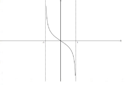
Figure 1: $\Lambda$ for the Klein Gordon equation.

One can deduce an ODE from (3), developing the symbol $\lambda_{h}(x,\xi)$ on $\Lambda$, i.e. on $\xi=d\varphi(x)$. One obtains a first term $a(x)$ independent of $\xi$ and a remainder, which turns out to be integrable in time as may be shown using some ideas of Ifrim-Tataru [16] and the $L^{2}$ estimates verified by $v$ and by the action of the Klainerman vector field on $v$. Essentially, one uses that operators whose symbols are localised in a neighbourhood of $\Lambda$ of size $O(\sqrt{h})$ have $\mathcal{L}(L^{2};L^{\infty})$ norms which are a $O(h^{-\frac{1}{4}-\sigma})$, for a small positive $\sigma$, instead of $O(h^{-\frac{1}{2}})$ as would follow from a direct application of the Sobolev injection. In this way, one proves that $v$ is solution of the equation

(4) $$D_{t}v=a(x)v+h\beta|v|^{2}v+\mbox{non characteristic terms}+\mbox{remainder of higher order in }h\,.$$

Then the idea is to eliminate non characteristic terms by a normal forms argument, introducing a new function $f$ which will be finally solution of an ordinary differential equation

(5) $$D_{t}f=a(x)f+h\beta|f|^{2}f+\mbox{remainder of higher order in }h\,.$$

From this equation, one easily derives an uniform control $L^{\infty}$ on $f$, and then on the starting solution $u$.

The analysis of the above ODE provides as well a one term asymptotic expansion of the solution of equation (2) (or, more generally of the solution (1)), as proved in the last section of this paper. This expansion shows that, in general, scattering does not hold, and that one has only modified scattering. This is in contrast with higher dimensional problems for the Klein-Gordon equation, where global solutions have at infinity the same behaviour as free solutions. In space dimension one, only few results were known regarding asymptotics of solution, including for the simpler equation

$$\Box u+u=\alpha u^{2}+\beta u^{3}+\mbox{order}\,4\,.$$

For this equation, Georgiev and Yordanov [10] proved that, when $\alpha=0$, the distance between the solution $u$ and linear solutions cannot tend to 0 when $t\rightarrow\infty$, but they do not obtain an asymptotic description of the solution (except for the particular case of sine-Gordon $\Box u+\sin u=0$, for which they use methods of "nonlinear scattering"). In [25], Lindblad and Soffer studied the scattering problem for long range nonlinearities, proving that for all prescribed asymptotic solutions there is a solution of the equation with such behavior, for some choice of initial data, and finding the complete asymptotic expansion of the solutions. Their method is based on the reduction of the long range phase effects to an ODE, via an appropriate ansatz. In [13], a sharp asymptotic behaviour of small solutions in the quadratic, semilinear case is proved by Hayashi and Naumkin, without the condition of compact support on initial data, using the method of normal forms of Shatah. In [4], Delort studied asymptotics in the quasi-linear case, obtaining a one term asymptotic expansion for the solution, under the assumption of small, compactly supported Cauchy data, and showing that in general the solution does not behave as in the linear case. The only other cases in dimension one for which the asymptotic behaviour is known concern nonlinearities studied by Moriyama in [26], where he showed that solutions have a free asymptotic behaviour, assuming the initial data to be sufficiently small and decaying at infinity.

1 Statement of the main results

The Cauchy problem we are considering is

(1.1) $$\begin{cases}&\Box u+u=P(u,\partial_{t}\partial_{x}u,\partial^{2}_{x}u\,;\partial_{t}u,\partial_{x}u)\\ &u(1,x)=\varepsilon u_{0}(x)\\ &\partial_{t}u(1,x)=\varepsilon u_{1}(x)\end{cases}\qquad t\geq 1\,,x\in\mathbb{R}$$

where $\Box:=\partial^{2}_{t}-\partial^{2}_{x}$ is the D’Alembert operator, $\varepsilon\in]0,1[$, $u_{0},u_{1}$ are smooth enough functions. $P$ denotes a homogeneous polynomial of degree three, with real constant coefficients, affine in $(\partial_{t}\partial_{x}u,\partial^{2}_{x}u)$. We can highlight this particular dependence on second derivatives following the approach of [4] and decomposing $P$ as

(1.2) $$P(u,\partial_{t}\partial_{x}u,\partial^{2}_{x}u\,;\partial_{t}u,\partial_{x}u)=P^{\prime}(u\,;\partial_{t}u,\partial_{x}u)+P^{\prime\prime}(u,\partial_{t}\partial_{x}u,\partial^{2}_{x}u\,;\partial_{t}u,\partial_{x}u)\,,$$

where $P^{\prime},P^{\prime\prime}$ are homogeneous polynomials of degree three, $P^{\prime\prime}$ linear in $(\partial_{t}\partial_{x}u,\partial^{2}_{x}u)$. Moreover

(1.3) $$\begin{split}P^{\prime}(X_{1};\,Y_{1},Y_{2})&=\sum_{k=0}^{3}i^{k}P_{k}^{\prime}(X_{1};-iY_{1},-iY_{2})\\ P^{\prime\prime}(X_{1},X_{2},X_{3};\,Y_{1},Y_{2})&=\sum_{k=0}^{2}i^{k}P_{k}^{\prime\prime}(X_{1},-X_{2},-X_{3};-iY_{1},-iY_{2})\end{split}$$

where $P_{k}^{\prime}$ is homogeneous of degree $k$ in $(Y_{1},Y_{2})$ and of degree $3-k$ in $X_{1}$, while $P_{k}^{\prime\prime}$ is homogeneous of degree 1 in $(X_{2},X_{3})$ and of degree $k$ in $(Y_{1},Y_{2})$. We denote $P_{k}=P^{\prime}_{k}+P^{\prime\prime}_{k}$. For $x\in]-1,1[$, define

(1.4) $$\begin{split}&\omega_{0}(x):=\frac{1}{\sqrt{1-x^{2}}}\,,\\ &\omega_{1}(x):=\frac{-x}{\sqrt{1-x^{2}}}\,,\end{split}$$

and

(1.5) $$\Phi(x):=P^{\prime}_{1}(1;\omega_{0}(x),\omega_{1}(x))+P^{\prime\prime}_{1}(1,\omega_{0}(x)\omega_{1}(x),\omega_{1}^{2}(x);\omega_{0}(x),\omega_{1}(x))+3P^{\prime}_{3}(1;\omega_{0}(x),\omega_{1}(x))\,.$$

Definition 1.1.

We say that the nonlinearity $P$ satisfies the null condition if and only if $\Phi\equiv 0$.

Our goal is to prove that there is a global solution of (1.1) when $\varepsilon$ is sufficiently small, $u_{0},u_{1}$ decay rapidly enough at infinity, and when the cubic nonlinearity satisfies the null condition. We state the main theorem below.

Theorem 1.2 (Main Theorem).

Suppose that the nonlinearity $P$ satisfies the null condition. Then there exists an integer $s$ sufficiently large, a positive small number $\sigma$, an $\varepsilon_{0}\in]0,1[$ such that, for any real valued $(u_{0},u_{1})\in H^{s+1}(\mathbb{R})\times H^{s}(\mathbb{R})$ satisfying

(1.6) $$\|u_{0}\|_{H^{s+1}}+\|u_{1}\|_{H^{s}}+\|xu_{0}\|_{H^{2}}+\|xu_{1}\|_{H^{1}}\leq 1\,,$$

for any $0<\varepsilon<\varepsilon_{0}$, the problem (1.1) has an unique solution $u\in C^{0}([1,+\infty[;H^{s+1})\cap C^{1}([1,+\infty[;H^{s})$. Moreover, there exists a $1$-parameter family of continuous function $a_{\varepsilon}:\mathbb{R}\rightarrow\mathbb{C}$, uniformly bounded and supported in $[-1,1]$, a function $(t,x)\rightarrow r(t,x)$ with values in $L^{2}(\mathbb{R})\cap L^{\infty}(\mathbb{R})$, bounded in $t\geq 1$, such that, for any $\varepsilon\in]0,\varepsilon_{0}]$, the global solution $u$ of (1.1) has the asymptotic expansion

(1.7) $$u(t,x)=\Re\left[\frac{\varepsilon}{\sqrt{t}}a_{\varepsilon}\left(\frac{x}{t}\right)\exp\left[it\varphi\left(\frac{x}{t}\right)+i\varepsilon^{2}\left|a_{\varepsilon}\left(\frac{x}{t}\right)\right|^{2}\Phi_{1}\left(\frac{x}{t}\right)\log t\right]\right]+\frac{\varepsilon}{t^{\frac{1}{2}+\sigma}}r(t,x)\,,$$

where $\varphi(x)=\sqrt{1-x^{2}}$, and

(1.8) $$\begin{split}\Phi_{1}(x)=\frac{1}{8}\langle\omega_{0}(x)\rangle^{-4}&\left[3P_{0}(1,\omega_{0}(x)\omega_{1}(x),\omega_{1}(x)^{2};\,\omega_{0}(x),\omega_{1}(x))\right.\\ &\left.+P_{2}(1,\omega_{0}(x)\omega_{1}(x),\omega_{1}(x)^{2};\,\omega_{0}(x),\omega_{1}(x))\right]\,,\end{split}$$

with $\langle x\rangle=\sqrt{1+x^{2}}$.

We denote by $Z$ the Klainerman vector field for the Klein-Gordon equation, that is $Z:=t\partial_{x}+x\partial_{t}$, and by $\Gamma$ a generic vector field in the set $\mathcal{Z}=\{Z,\partial_{t},\partial_{x}\}$. The most remarkable properties of these vector fields are the commutation with the linear part of the equation in (1.1), namely

(1.9) $$[\Box+1,\Gamma]=0\,,$$

and the fact that they act like a derivation on the cubic nonlinearity. Using the notation $D=\frac{1}{i}\partial$, we also denote by $W^{t,\rho,\infty}$ a modified Sobolev space, made by functions $t\rightarrow\psi(t,\cdot)$ defined on an interval, such that $\langle D_{x}\rangle^{\rho-i}D^{i}_{t}u\in L^{\infty}$, for $i\leq 2$, with the norm

(1.10) $$\|\psi(t,\cdot)\|_{W^{t,\rho,\infty}(\mathbb{R})}:=\sum_{i=0}^{2}\|\langle D_{x}\rangle^{\rho-i}D^{i}_{t}\psi(t,\cdot)\|_{L^{\infty}(\mathbb{R})}\,.$$

The proof of the main theorem is based on a bootstrap argument. In other words, we shall prove that we are able to propagate some a priori estimates made on a solution $u$ of (1.1) on some interval $[1,T]$, for some $T>1$ fixed, as stated in the following theorem.

Theorem 1.3 (Bootstrap Theorem).

There exist two integers $s,\rho$ large enough, $s\gg\rho$, an $\varepsilon_{0}\in]0,1[$ sufficiently small, and two constants $A,B>0$ sufficiently large such that, for any $0<\varepsilon<\varepsilon_{0}$, if $u$ is a solution of (1.1) on some interval $[1,T]$, for $T>1$ fixed, and satisfies

(1.11a) $$\|u(t,\cdot)\|_{W^{t,\rho,\infty}}\leq A\varepsilon t^{-\frac{1}{2}}$$

(1.11b) $$\|Zu(t,\cdot)\|_{H^{1}}\leq B\varepsilon t^{\sigma}\,,\qquad\|\partial_{t}Zu(t,\cdot)\|_{L^{2}}\leq B\varepsilon t^{\sigma}$$

(1.11c) $$\|u(t,\cdot)\|_{H^{s}}\leq B\varepsilon t^{\sigma}\,,\qquad\hskip 8.5359pt\|\partial_{t}u(t,\cdot)\|_{H^{s-1}}\leq B\varepsilon t^{\sigma}\,,$$

for every $t\in[1,T]$, for some $\sigma\geq 0$ small, then it verifies also

(1.12a) $$\|u(t,\cdot)\|_{W^{t,\rho,\infty}}\leq\frac{A}{2}\varepsilon t^{-\frac{1}{2}}$$

(1.12b) $$\|Zu(t,\cdot)\|_{H^{1}}\leq\frac{B}{2}\varepsilon t^{\sigma}\,,\qquad\|\partial_{t}Zu(t,\cdot)\|_{L^{2}}\leq\frac{B}{2}\varepsilon t^{\sigma}$$

(1.12c) $$\|u(t,\cdot)\|_{H^{s}}\leq\frac{B}{2}\varepsilon t^{\sigma}\,,\qquad\hskip 8.5359pt\|\partial_{t}u(t,\cdot)\|_{H^{s-1}}\leq\frac{B}{2}\varepsilon t^{\sigma}\,.$$

In section 2 we show that energy bounds (1.11b), (1.11c) can be propagated, simply recalling an energy inequality obtained by Hörmander in [15] for a solution $u$ of a quasi-linear Klein-Gordon equation, and applying it to $\partial^{s-1}_{x}u$ and $Zu$. Sections from 3 to 5 concern instead the proof of the uniform estimate’s propagation. Furthermore, in section 5 we derive also the asymptotic behaviour of the solution $u$.

To conclude, we can mention that we will mainly focus on not very high frequencies, for it is easier to control what happens for very large frequencies which correspond to points on $\Lambda$ in figure 1 close to vertical asymptotic lines. This is justified by the fact that contributions of frequencies of the solution larger than $h^{-\beta}$, for a small positive $\beta$, have $L^{2}$ norms of order $O(h^{N})$ if $s\beta\gg N$, assuming small $H^{s}$ estimates on $v$. In this way, most of the analysis is reduced to frequencies lower than $h^{-\beta}$.

2 Generalised energy estimates

With notations introduced in the previous section, we define

(2.1) $$E_{0}(t,u)=\big{(}\|\partial_{t}u(t,\cdot)\|_{L^{2}}^{2}+\|\partial_{x}u(t,\cdot)\|_{L^{2}}^{2}+\|u(t,\cdot)\|_{L^{2}}^{2}\big{)}^{1/2}$$

as the square root of the energy associated to the solution $u$ of (1.1) at time $t$, and $E^{\Gamma}_{N}(t,u)=\displaystyle\sum_{k=0}^{N}\big{(}E_{0}(t,\Gamma^{k}u)^{2}\big{)}^{1/2}$, for a fixed $\Gamma$. The goal of this section is to obtain an energy inequality involving $E^{\Gamma}_{N}(t,u)$. In particular, since the aim is to propagate a priori energy bounds on $u$, i.e. $\|u(t,\cdot)\|_{H^{s}}$, $\|\partial_{t}u(t,\cdot)\|_{H^{s-1}}$, $\|Zu(t,\cdot)\|_{H^{1}}$ and $\|\partial_{t}Zu(t,\cdot)\|_{L^{2}}$, we will consider on one hand $E^{\partial_{x}}_{s-1}(t,u)$ where all $\Gamma$ are equal to $\partial_{x}$, and on the other $E^{Z}_{1}(t,u)$ where $\Gamma=Z$. Often in what follows we will denote partial derivatives with respect to $t$ and $x$ respectively by $\partial_{0}$ and $\partial_{1}$.

We will use the following result, which concerns the specific energy inequality for the Klein-Gordon equation in the quasi-linear case, and which is presented here without proof (see lemma 7.4.1 in [15] for further details).

Lemma 2.1.

Let u be a solution of

(2.2) $$\Box u+u+\gamma^{01}\partial_{0}\partial_{1}u+\gamma^{11}\partial_{1}^{2}u+\gamma^{0}\partial_{0}u+\gamma^{1}\partial_{1}u=f\,,$$

where functions $\gamma^{ij}=\gamma^{ij}(t,x)$, $\gamma^{j}=\gamma^{j}(t,x)$ are smooth, such that $\displaystyle\sum_{i,j=0}^{1}|\gamma^{ij}|+|\gamma^{j}|\leq\frac{1}{2}$. Then,

(2.3) $$E_{0}(t,u)\leq C\big{[}E_{0}(1,u)+\int_{1}^{t}\|f(\tau,\cdot)\|_{L^{2}}d\tau\big{]}\exp\big{(}\int_{1}^{t}C(\tau)\,d\tau\big{)}\,,$$

where $C(\tau):=\displaystyle\sum_{i,j,h=0}^{1}\displaystyle\sup_{x}\left(|\partial_{h}\gamma^{ij}(\tau,x)|+|\partial_{h}\gamma^{j}(\tau,x)|\right)$.

We can rewrite the equation in (1.1) in the same form as in lemma 2.1, especially highlighting the linear dependence on second derivatives,

(2.4) $$\Box u+u+\gamma^{01}\partial_{0}\partial_{1}u+\gamma^{11}\partial_{1}^{2}u+\gamma^{0}\partial_{0}u+\gamma^{1}\partial_{1}u=0\,,$$

where coefficients $\gamma^{ij},\gamma^{j}$ are homogeneous polynomials of degree two in $(u,\partial_{0}u,\partial_{1}u)$. Let us apply $\partial^{s^{\prime}}_{1}$, $s^{\prime}:=s-1$, to this equation. If $u$ is a solution of (2.4), then $\partial^{s^{\prime}}_{1}u$ satisfies

(2.5) $$\Box\partial^{s^{\prime}}_{1}u+\partial^{s^{\prime}}_{1}u+\partial^{s^{\prime}}_{1}\big{(}\gamma^{01}\partial_{0}\partial_{1}u+\gamma^{11}\partial_{1}^{2}u+\gamma^{0}\partial_{0}u+\gamma^{1}\partial_{1}u\big{)}=0\,,$$

and applying the Leibniz rule, we obtain that $\partial^{s^{\prime}}_{1}u$ is solution of the equation

(2.6) $$\Box\partial^{s^{\prime}}_{1}u+\partial^{s^{\prime}}_{1}u+\gamma^{01}\partial_{0}\partial_{1}(\partial^{s^{\prime}}_{1}u)+\gamma^{11}\partial_{1}^{2}(\partial^{s^{\prime}}_{1}u)+\gamma^{0}\partial_{0}(\partial^{s^{\prime}}_{1}u)+\gamma^{1}\partial_{1}(\partial^{s^{\prime}}_{1}u)=f^{s^{\prime}}\,,$$

where $f^{s^{\prime}}$ is a linear combination of terms of the form

(2.7) $$\begin{split}&(\partial_{1}^{s^{\prime}_{1}}\partial_{i}^{\alpha_{1}}u)\,(\partial_{1}^{s^{\prime}_{2}}\partial_{j}^{\alpha_{2}}u)\,(\partial_{1}^{s^{\prime}_{3}}\partial^{2}_{ij}u)\ ,\\ &(\partial_{1}^{s^{\prime}_{1}}\partial_{i}^{\alpha_{1}}u)\,(\partial_{1}^{s^{\prime}_{2}}\partial_{j}^{\alpha_{2}}u)\,(\partial_{1}^{s^{\prime}_{3}}\partial_{h}u)\,,\end{split}$$

for $i,j,h,\alpha_{1},\alpha_{2}=0,1$, $s^{\prime}_{1}+s^{\prime}_{2}+s^{\prime}_{3}=s^{\prime}$, $s^{\prime}_{3}<s^{\prime}$. So taking the $L^{2}$ norm and observing that at most one index $s^{\prime}_{j}$ can be larger than $s^{\prime}/2$, we have

(2.8) $$\|f^{s^{\prime}}(t,\cdot)\|_{L^{2}}\leq\Big{(}\sum_{\begin{subarray}{c}i+j=0\\ j\leq 2\end{subarray}}^{[\frac{s^{\prime}}{2}]+2}\|\partial^{i}_{x}\partial^{j}_{t}u(t,\cdot)\|^{2}_{L^{\infty}}\Big{)}E^{\partial_{1}}_{s^{\prime}}(t,u)\leq\|u(t,\cdot)\|^{2}_{W^{t,\rho,\infty}}E^{\partial_{1}}_{s^{\prime}}(t,u)\,,$$

for a $\rho\geq[\frac{s^{\prime}}{2}]+3$. Rewriting inequality (2.3) for $\partial^{s^{\prime}}_{1}u$, where $s^{\prime}=s-1$ and $C(\tau)\leq\|u(\tau,\cdot)\|^{2}_{W^{t,2,\infty}}$, we obtain

(2.9) $$E^{\partial_{1}}_{s-1}(t,u)\leq C\left[E^{\partial_{1}}_{s-1}(1,u)+\int_{1}^{t}\|u(\tau,\cdot)\|^{2}_{W^{t,\rho,\infty}}E^{\partial_{1}}_{s-1}(\tau,u)d\tau\right]\exp\left(\int_{1}^{t}\|u(\tau,\cdot)\|^{2}_{W^{t,2,\infty}}d\tau\right).$$

On the other hand, we want to obtain an analogous of (2.9) for $E_{1}^{Z}(t,u)$. Applying $Z$ to (2.4), Leibniz rule and commutations, we derive that $Zu$ is solution of the equation

(2.10) $$\Box Zu+Zu+\gamma^{01}\partial_{0}\partial_{1}Zu+\gamma^{11}\partial_{1}^{2}Zu+\gamma^{0}\partial_{0}Zu+\gamma^{1}\partial_{1}Zu=f^{Z}\,,$$

where $f^{Z}$ is linear combination of $[\gamma^{ij}\partial^{2}_{ij},Z]u$ and $[\gamma^{h}\partial_{h},Z]u$. We calculate for instance the term $[\gamma^{01}\partial^{2}_{01},Z]u$ and we find that it is equal to $-(Z\gamma^{01})\partial^{2}_{01}u-\gamma^{01}[\partial^{2}_{01},Z]u$, that is a linear combination of

(2.11) $$\begin{split}&(\partial^{\alpha_{1}}_{i}u)(\partial^{\alpha_{2}}_{j}Zu)(\partial^{2}_{01}u)\,,\\ &(\partial^{\alpha_{1}}_{i}u)(\partial^{\alpha_{2}}_{j}u)(\partial^{2}_{hk}u)\,,\end{split}$$

for $i,j,h,k,\alpha_{1},\alpha_{2}=0,1$. Therefore, the $L^{2}$ norm of $f^{Z}$ can be estimated as follows

(2.12) $$\|f^{Z}(t,\cdot)\|_{L^{2}}\leq\Big{(}\sum_{i+j=0}^{2}\|\partial^{i}_{x}\partial^{j}_{t}u(t,\cdot)\|^{2}_{L^{\infty}}\Big{)}E^{Z}_{1}(t,u)\leq\|u(t,\cdot)\|^{2}_{W^{t,3,\infty}}E^{Z}_{1}(t,u)\,,$$

and applying lemma 2.1 for $Zu$, we derive

(2.13) $$E^{Z}_{1}(t,u)\leq C\left[E^{Z}_{1}(1,u)+\int_{1}^{t}\|u(\tau,\cdot)\|^{2}_{W^{t,3,\infty}}E_{1}^{Z}(\tau,\cdot)\,d\tau\right]\exp\left(\int_{1}^{t}\|u(s,\cdot)\|^{2}_{W^{t,2,\infty}}ds\right)\,.$$

Remark.

To make the above proof fully correct, one should chek as well that the energy of $Zu$ is actually finite at every fixed positive time. One may do that either using that the vector field $Z$ is the infinitesimal generator of the action on the equation of a one parameter group, along the lines of appendix A.2 in [1]. Alternatively, one may instead exploit finite propagation speed, remarking that if the data are cut off on a compact set, the solution remains compactly supported at every fixed time, so that the energy of $Zu$ is actually finite, and that the bounds we get are uniform in terms of the cut off.

Proposition 2.2 (Propagation of Energy Estimates).

There exist an integer $s$ large enough, a $\rho\geq[\frac{s-1}{2}]+3$, $\rho\ll s$, an $\varepsilon_{0}\in]0,1[$ sufficiently small, a small $\sigma\geq 0$, and two constants $A,B>0$ sufficiently large such that, for any $0<\varepsilon<\varepsilon_{0}$, if $u$ is a solution of (1.1) on some interval $[1,T]$, for $T>1$ fixed, and satisfies

(2.14a) $$\|u(t,\cdot)\|_{W^{t,\rho,\infty}}\leq A\varepsilon t^{-\frac{1}{2}}\,,$$

(2.14b) $$E_{s-1}^{\partial_{1}}(t,u)\leq B\varepsilon t^{\sigma}\,,$$

(2.14c) $$E_{1}^{Z}(t,u)\leq B\varepsilon t^{\sigma}\,,$$

for every $t\in[1,T]$, then it verifies also

(2.15a) $$E_{s-1}^{\partial_{1}}(t,u)\leq\frac{B}{2}\varepsilon t^{\sigma}\,,$$

(2.15b) $$E_{1}^{Z}(t,u)\leq\frac{B}{2}\varepsilon t^{\sigma}\,.$$

Proof.

Both estimates (2.14b) and (2.14c) can be propagated injecting a priori estimates (2.14) in energy inequalities (2.9) and (2.13) derived before, obtaining

$$\begin{split}E^{\partial_{1}}_{s-1}(t,u)&\leq C\Big{[}E^{\partial_{1}}_{s-1}(1,u)+A^{2}B\varepsilon^{3}\int_{1}^{t}\tau^{-1+\sigma}d\tau\Big{]}\leq CE^{\partial_{1}}_{s-1}(1,u)+\frac{A^{2}BC\varepsilon^{3}}{\sigma}t^{\sigma}\,,\\ E^{Z}_{1}(t,u)&\leq C\Big{[}E^{Z}_{1}(1,u)+A^{2}B\varepsilon^{3}\int_{1}^{t}\tau^{-1+\sigma}d\tau\Big{]}\leq CE^{Z}_{1}(1,u)+\frac{A^{2}BC\varepsilon^{3}}{\sigma}t^{\sigma}\,.\end{split}$$

Then we can choose $B>0$ sufficiently large such that $CE^{\partial_{1}}_{s-1}(1,u)+CE_{1}^{Z}(1,u)\leq\frac{B}{4}\varepsilon$, and $\varepsilon_{0}>0$ sufficiently small such that $\frac{A^{2}C\varepsilon^{2}}{\sigma}\leq\frac{1}{4}$, to obtain (2.15a), (2.15b).

3 Semiclassical Pseudo-differential Operators.

As told in the introduction, in order to prove an $L^{\infty}$ estimate on $u$ and on its derivatives we need to reformulate the starting problem (1.1) in term of an ODE satisfied by a new function $v$ obtained from $u$, and this will strongly use the semiclassical pseudo-differential calculus. In the following two subsections, we introduce this semiclassical environment, defining classes of symbols and operators we shall use and several useful properties, some of which are stated without proof. More details can be found in [8] and [37].

3.1 Definitions and Composition Formula

Definition 3.1.

An order function on $\mathbb{R}\times\mathbb{R}$ is a smooth map from $\mathbb{R}\times\mathbb{R}$ to $\mathbb{R}_{+}$ : $(x,\xi)\rightarrow M(x,\xi)$ such that there exist $N_{0}\in\mathbb{N}$, $C>0$ and for any $(x,\xi),(y,\eta)\in\mathbb{R}\times\mathbb{R}$

(3.1) $$M(y,\eta)\leq C\langle x-y\rangle^{N_{0}}\langle\xi-\eta\rangle^{N_{0}}M(x,\xi)\,,$$

where $\langle x\rangle=\sqrt{1+x^{2}}$.

Examples of order functions are $\langle x\rangle$, $\langle\xi\rangle$, $\langle x\rangle\langle\xi\rangle$.

Definition 3.2.

Let M be an order function on $\mathbb{R}\times\mathbb{R}$, $\beta\geq 0$, $\delta\geq 0$. One denotes by $S_{\delta,\beta}(M)$ the space of smooth functions

$$(x,\xi,h) \rightarrow a(x,\xi,h)$$

$$\mathbb{R}\times\mathbb{R}\times]0,1] \rightarrow\mathbb{C}$$

satisfying for any $\alpha_{1},\alpha_{2},k,N\in\mathbb{N}$ bounds

(3.2) $$|\partial_{x}^{\alpha_{1}}\partial_{\xi}^{\alpha_{2}}(h\partial_{h})^{k}a(x,\xi,h)|\leq CM(x,\xi)\,h^{-\delta(\alpha_{1}+\alpha_{2})}(1+\beta h^{\beta}|\xi|)^{-N}\,.$$

A key role in this paper will be played by symbols $a$ verifying (3.2) with $M(x,\xi)=\langle\frac{x+f(\xi)}{\sqrt{h}}\rangle^{-N}$, for $N\in\mathbb{N}$ and a certain smooth function $f(\xi)$. This function $M$ is no longer an order function because of the term $h^{-\frac{1}{2}}$ but nevertheless we continue to keep the notation $a\in S_{\delta,\beta}(\langle\frac{x+f(\xi)}{\sqrt{h}}\rangle^{-N})$.

Definition 3.3.

We will say that $a(x,\xi)$ is a symbol of order $r$ if $a\in S_{\delta,\beta}(\langle\xi\rangle^{r})$, for some $\delta\geq 0$, $\beta\geq 0$.

Let us observe that when $\beta>0$, the symbol decays rapidly in $h^{\beta}|\xi|$, which implies the following inclusion for $r\geq 0$

(3.3) $$S_{\delta,\beta}(\langle\xi\rangle^{r})\subset h^{-\beta r}S_{\delta,\beta}(1)\,,$$

which will be often use in all the paper. This means that, up to a small loss in $h$, this type of symbols can be always considered as symbols of order zero. In the rest of the paper we will not indicate explicitly the dependence of symbols on $h$, referring to $a(x,\xi,h)$ simply as $a(x,\xi)$.

Definition 3.4.

Let $a\in S_{\delta,\beta}(M)$ for some order function $M$, some $\delta\geq 0$, $\beta\geq 0$.

1. We can define the Weyl quantization of $a$ to be the operator $Op_{h}^{w}(a)=a^{w}(x,hD)$ acting on $u\in\mathcal{S}(\mathbb{R})$ by the formula :

   (3.4) $$Op_{h}^{w}(a(x,\xi))u(x)=\frac{1}{2\pi h}\int_{\mathbb{R}}\int_{\mathbb{R}}e^{\frac{i}{h}(x-y)\xi}a(\frac{x+y}{2},\xi)\,u(y)\;dyd\xi\,;$$

2. We define also the standard quantization :

   (3.5) $$Op_{h}(a(x,\xi))u(x)=\frac{1}{2\pi h}\int_{\mathbb{R}}\int_{\mathbb{R}}e^{\frac{i}{h}(x-y)\xi}a(x,\xi)\,u(y)\;dyd\xi\,.$$

It is clear from the definition that the two quantizations coincide when the symbol does not depend on $x$.

We introduce also a semiclassical version of Sobolev spaces, on which is more natural to consider the action of above operators.

Definition 3.5.

1. Let $\rho\in\mathbb{N}$. We define the semiclassical Sobolev space $W^{\rho,\infty}_{h}(\mathbb{R})$ as the space of families $(v_{h})_{h\in]0,1]}$ of tempered distributions, such that $\langle hD\rangle^{\rho}v_{h}:=Op_{h}(\langle\xi\rangle^{\rho})v_{h}$ is a bounded family of $L^{\infty}$, i.e.

   (3.6) $$W_{h}^{\rho,\infty}(\mathbb{R}):=\left\{v_{h}\in\mathcal{S}^{\prime}(\mathbb{R})\,\Big{|}\,\sup_{h\in]0,1]}\|\langle hD\rangle^{\rho}v_{h}\|_{L^{\infty}(\mathbb{R})}<+\infty\right\}\,.$$

2. Let $s\in\mathbb{R}$. We define the semiclassical Sobolev space $H^{s}_{h}(\mathbb{R})$ as the space of families $(v_{h})_{h\in]0,1]}$ of tempered distributions such that $\langle hD\rangle^{s}v_{h}:=Op_{h}(\langle\xi\rangle^{s})v_{h}$ is a bounded family of $L^{2}$, i.e.

   (3.7) $$H^{s}_{h}(\mathbb{R}):=\left\{v_{h}\in\mathcal{S}^{\prime}(\mathbb{R})\,\Big{|}\,\sup_{h\in]0,1]}\int_{\mathbb{R}}(1+|h\xi|^{2})^{s}|\hat{v}_{h}(\xi)|^{2}\,d\xi<+\infty\right\}\,.$$

For future references, we write down the semiclassical Sobolev injection,

(3.8) $$\|v_{h}\|_{W_{h}^{\rho,\infty}}\leq C_{\theta}h^{-\frac{1}{2}}\|v_{h}\|_{H^{\rho+\frac{1}{2}+\theta}_{h}}\,,\qquad\forall\theta>0\,.$$

The following two propositions are stated without proof. They concern the adjoint and the composition of pseudo-differential operators we are considering, and a full detailed treatment is provided in chapter 7 of [8], or in chapter 4 of [37].

Proposition 3.6 (Self-Adjointness).

If $a$ is a real symbol, its Weyl quantization is self-adjoint,

(3.9) $$\big{(}Op_{h}^{w}(a)\big{)}^{*}=Op_{h}^{w}(a)\,.$$

Proposition 3.7 (Composition for Weyl quantization).

Let $a,b\in\mathcal{S}(\mathbb{R})$. Then

(3.10) $$Op_{h}^{w}(a)\circ Op_{h}^{w}(b)=Op_{h}^{w}(a\sharp b)\,,$$

where

(3.11) $$a\sharp b\,(x,\xi):=\frac{1}{(\pi h)^{2}}\int_{\mathbb{R}}\int_{\mathbb{R}}\int_{\mathbb{R}}\int_{\mathbb{R}}e^{\frac{2i}{h}\sigma(y,\eta;\,z,\zeta)}a(x+z,\xi+\zeta)b(x+y,\xi+\eta)\;dyd\eta dzd\zeta$$

and

$$\sigma(y,\eta;\,z,\zeta)=\eta z-y\zeta\,.$$

It is often useful to derive an asymptotic expansion for $a\sharp b$, which allows easier computations than the integral formula (3.11). This expansion is usually obtained by applying the stationary phase argument when $a,b\in S_{\delta,\beta}(M)$, $\delta\in[0,\frac{1}{2}[$ (as shown in [37]). Here we provide an expansion at any order even when one of two symbols belongs to $S_{\frac{1}{2},\beta_{1}}(M)$ (still having the other in $S_{\delta,\beta_{2}}(M)$ for $\delta<\frac{1}{2}$, and $\beta_{1},\beta_{2}$ either equal or, if not, one of them equal to zero), whose proof is based on the Taylor development of symbols $a,b$, and can be found in detail in the appendix.

Proposition 3.8.

Let $a\in S_{\delta_{1},\beta_{1}}(M_{1})$, $b\in S_{\delta_{2},\beta_{2}}(M_{2})$, $\delta_{1},\delta_{2}\in[0,\frac{1}{2}]$, $\delta_{1}+\delta_{2}<1$, $\beta_{1},\beta_{2}\geq 0$ such that

(3.12) $$\beta_{1}=\beta_{2}\geq 0\qquad\mbox{or}\qquad\big{[}\beta_{1}\neq\beta_{2}\,\mbox{and}\,\beta_{i}=0\,,\beta_{j}>0\,,i\neq j\in\{1,2\}\big{]}\,.$$

Then $a\sharp b\in S_{\delta,\beta}(M_{1}M_{2})$, where $\delta=\max\{\delta_{1},\delta_{2}\}$, $\beta=\max\{\beta_{1},\beta_{2}\}$. Moreover,

(3.13) $$a\sharp b=ab+\frac{h}{2i}\{a,b\}+\sum_{\begin{subarray}{c}\alpha=(\alpha_{1},\alpha_{2})\\ 2\leq|\alpha|\leq k\end{subarray}}\left(\frac{h}{2i}\right)^{|\alpha|}\frac{(-1)^{\alpha_{1}}}{\alpha!}\partial^{\alpha_{1}}_{x}\partial_{\xi}^{\alpha_{2}}a\,\partial_{x}^{\alpha_{2}}\partial_{\xi}^{\alpha_{1}}b+r_{k}\,,$$

where $\{a,b\}=\partial_{\xi}a\partial_{x}b-\partial_{\xi}b\partial_{x}a$, $r_{k}\in h^{(k+1)(1-(\delta_{1}+\delta_{2}))}S_{\delta,\beta}(M_{1}M_{2})$ and

(3.14) $$\begin{split}r_{k}(x,\xi)=\,\left(\frac{h}{2i}\right)^{k+1}\frac{k+1}{(\pi h)^{2}}\sum_{\begin{subarray}{c}\alpha=(\alpha_{1},\alpha_{2})\\ |\alpha|=k+1\end{subarray}}\frac{(-1)^{\alpha_{1}}}{\alpha!}\int_{\mathbb{R}^{4}}e^{\frac{2i}{h}(\eta z-y\zeta)}\Big{\{}&\int_{0}^{1}\partial_{x}^{\alpha_{1}}\partial_{\xi}^{\alpha_{2}}a(x+tz,\xi+t\zeta)(1-t)^{k}dt\\ &\times\partial_{y}^{\alpha_{2}}\partial_{\eta}^{\alpha_{1}}b(x+y,\xi+\eta)\Big{\}}\,dyd\eta dzd\zeta\,.\end{split}$$

More generally, if $h^{(k+1)\delta_{1}}\partial^{\alpha}a\in S_{\delta_{1},\beta_{1}}(M^{k+1}_{1})$, $h^{(k+1)\delta_{2}}\partial^{\alpha}b\in S_{\delta_{2},\beta_{2}}(M^{k+1}_{2})$, for $|\alpha|=k+1$, for order functions $M_{1}^{k+1},M_{2}^{k+1}$, then $r_{k}\in h^{(k+1)(1-(\delta_{1}+\delta_{2}))}S_{\delta,\beta}(M^{k+1}_{1}M^{k+1}_{2})$.

Remark.

Observe that

(3.15) $$a\sharp b=ab+\frac{h}{2i}\{a,b\}+\left(\frac{h}{2i}\right)^{2}\left[\frac{1}{2}\partial^{2}_{x}a\partial^{2}_{\xi}b+\frac{1}{2}\partial^{2}_{\xi}a\partial^{2}_{x}b-\partial_{x}\partial_{\xi}a\partial_{x}\partial_{\xi}b\right]+r^{a\sharp b}_{2}\,,$$

so the contribution of order two (and all other contributions of even order) disappears when we calculate the symbol associated to a commutator

(3.16) $$a\sharp b-b\sharp a=\frac{h}{i}\{a,b\}+r_{2}\,,$$

where $r_{2}=r_{2}^{a\sharp b}-r_{2}^{b\sharp a}\in h^{3(1-(\delta_{1}+\delta_{2}))}S_{\delta,\beta}(M_{1}M_{2})$.

The result of proposition 3.8 is still true also when one of order functions, or both, has the form $\langle\frac{x+f(\xi)}{\sqrt{h}}\rangle^{-1}$, for a smooth function $f(\xi)$, $f^{\prime}(\xi)$ bounded, as stated below and proved as well in the appendix.

Lemma 3.9.

Let $f(\xi)$ be a smooth function, $f^{\prime}(\xi)$ bounded. Consider $a\in S_{\delta_{1},\beta_{1}}(\langle\frac{x+f(\xi)}{\sqrt{h}}\rangle^{-d})$, $d\in\mathbb{N}$, and $b\in S_{\delta_{2},\beta_{2}}(M)$, for $M$ order function or $M(x,\xi)=\langle\frac{x+f(\xi)}{\sqrt{h}}\rangle^{-l}$, $l\in\mathbb{N}$, some $\delta_{1}\in[0,\frac{1}{2}]$, $\delta_{2}\in[0,\frac{1}{2}[$, $\beta_{1},\beta_{2}\geq 0$ as in (3.12). Then $a\sharp b\in S_{\delta,\beta}(\langle\frac{x+f(\xi)}{\sqrt{h}}\rangle^{-d}M)$, where $\delta=\max\{\delta_{1},\delta_{2}\}$, $\beta=\max\{\beta_{1},\beta_{2}\}$, and the asymptotic expansion (3.13) holds, with $r_{k}$ given by (3.14), $r_{k}\in h^{(k+1)(1-(\delta_{1}+\delta_{2}))}S_{\delta,\beta}(\langle\frac{x+f(\xi)}{\sqrt{h}}\rangle^{-d}M)$.
More generally, if $h^{(k+1)\delta_{1}}\partial^{\alpha}a\in S_{\delta_{1},\beta_{1}}(\langle\frac{x+f(\xi)}{\sqrt{h}}\rangle^{-d^{\prime}})$ and $h^{(k+1)\delta_{2}}\partial^{\alpha}b\in S_{\delta_{2},\beta_{2}}(M^{k+1})$, $|\alpha|=k+1$, $M^{k+1}$ order function or $M^{k+1}(x,\xi)=\langle\frac{x+f(\xi)}{\sqrt{h}}\rangle^{-l^{\prime}}$, for others $d^{\prime},l^{\prime}\in\mathbb{N}$, then $r_{k}\in h^{(k+1)(1-(\delta_{1}+\delta_{2}))}S_{\delta,\beta}(\langle\frac{x+f(\xi)}{\sqrt{h}}\rangle^{-d^{\prime}}M^{k+1})$.

3.2 Some Technical Estimates

This subsection is mostly devoted to the introduction of some technical results about symbols and operators we will often use in the entire paper, first of all continuity on Sobolev spaces. We also introduce multi-linear quantizations which will be used in the next section (and which are fully described in [6]), especially because they make our notations easier and clearer at first. Moreover, from now on we follow the notation $p(\xi):=\sqrt{1+\xi^{2}}$.

The first statement is about continuity on spaces $H^{s}_{h}(\mathbb{R})$, and generalises theorem 7.11 in [8]. The second statement concerns instead a result of continuity from $L^{2}$ to $W_{h}^{\rho,\infty}$. In the spirit of [16] for the Schrödinger equation, it allows to pass from uniform norms to the $L^{2}$ norm losing only a power $h^{-\frac{1}{4}-\sigma}$ for a small $\sigma>0$, and not a $h^{-\frac{1}{2}}$ as for the Sobolev injection.

Proposition 3.10 (Continuity on $H^{s}_{h}$).

Let $s\in\mathbb{R}$. Let $a\in S_{\delta,\beta}(\langle\xi\rangle^{r})$, $r\in\mathbb{R}$, $\delta\in[0,\frac{1}{2}]$, $\beta\geq 0$. Then $Op_{h}^{w}(a)$ is uniformly bounded : $H^{s}_{h}(\mathbb{R})\rightarrow H^{s-r}_{h}(\mathbb{R})$, and there exists a positive constant $C$ independent of $h$ such that

(3.17) $$\|Op_{h}^{w}(a)\|_{\mathcal{L}(H^{s}_{h};H^{s-r}_{h})}\leq C\,,\qquad\forall h\in]0,1]\,.$$

Proposition 3.11 (Continuity from $L^{2}$ to $W_{h}^{\rho,\infty}$).

Let $\rho\in\mathbb{N}$. Let $a\in S_{\delta,\beta}(\langle\frac{x+p^{\prime}(\xi)}{\sqrt{h}}\rangle^{-1})$, $\delta\in[0,\frac{1}{2}]$, $\beta>0$. Then $Op_{h}^{w}(a)$ is bounded : $L^{2}(\mathbb{R})\rightarrow W_{h}^{\rho,\infty}(\mathbb{R})$, and there exists a positive constant $C$ independent of $h$ such that

(3.18) $$\|Op_{h}^{w}(a)\|_{\mathcal{L}(L^{2};W_{h}^{\rho,\infty})}\leq Ch^{-\frac{1}{4}-\sigma}\,,\qquad\forall h\in]0,1]\,,$$

where $\sigma>0$ depends linearly on $\beta$.

Proof.

Firstly, remark that thanks to symbolic calculus of lemma 3.9, to estimate the $W_{h}^{k,\infty}$ norm of an operator whose symbol is rapidly decaying in $|h^{\beta}\xi|$ corresponds actually to estimate the $L^{\infty}$ norm of an operator associated to another symbol (namely, $\tilde{a}(x,\xi)=\langle\xi\rangle^{k}a(x,\xi)$) which is still in the same class as $a$, up to a small loss on $h$, of order $h^{-k\beta}$.

From the definition of $Op_{h}^{w}(a)v$, and using thereafter integration by part, Cauchy-Schwarz inequality, and Young’s inequality for convolutions, we derive what follows :

(3.19) $$\begin{split}&|Op_{h}^{w}(a)v|=\\ &=\left|\frac{1}{2\pi}\int_{\mathbb{R}}\int_{\mathbb{R}}e^{i(\frac{x}{\sqrt{h}}-y)\xi}a(\frac{x+\sqrt{h}y}{2},\sqrt{h}\xi)v(\sqrt{h}y)\,dyd\xi\right|\\ &=\left|\frac{1}{(2\pi)^{2}\sqrt{h}}\int_{\mathbb{R}}\hat{v}(\frac{\eta}{\sqrt{h}})d\eta\int_{\mathbb{R}}\int_{\mathbb{R}}e^{i(\frac{x}{\sqrt{h}}-y)\xi+i\eta y}a(\frac{x+\sqrt{h}y}{2},\sqrt{h}\xi)\,dyd\xi\right|\\ &\leq\left|\frac{1}{(2\pi)^{2}\sqrt{h}}\int_{\mathbb{R}}\hat{v}(\frac{\eta}{\sqrt{h}})\int_{\mathbb{R}}\int_{\mathbb{R}}\left(\frac{1-i(\frac{x}{\sqrt{h}}-y)\partial_{\xi}}{1+(\frac{x}{\sqrt{h}}-y)^{2}}\right)^{2}\left(\frac{1+i(\xi-\eta)\partial_{y}}{1+(\xi-\eta)^{2}}\right)^{2}\left[e^{i(\frac{x}{\sqrt{h}}-y)\xi+i\eta y}\right]\right.\\ &\left.\hskip 14.22636pt\times\,a(\frac{x+\sqrt{h}y}{2},\sqrt{h}\xi)\,dyd\xi d\eta\right|\\ &\leq\frac{C}{\sqrt{h}}\int_{\mathbb{R}}\left|\hat{v}(\frac{\eta}{\sqrt{h}})\right|\int_{\mathbb{R}}\int_{\mathbb{R}}\langle\frac{x}{\sqrt{h}}-y\rangle^{-2}\langle\xi-\eta\rangle^{-2}\langle h^{\beta}\sqrt{h}\xi\rangle^{-N}\Big{\langle}\frac{\frac{x+\sqrt{h}y}{2}+p^{\prime}(\sqrt{h}\xi)}{\sqrt{h}}\Big{\rangle}^{-1}dyd\xi d\eta\\ &\leq\frac{C}{\sqrt{h}}\left\|\hat{v}(\frac{\eta}{\sqrt{h}})\right\|_{L^{2}_{\eta}}\|\langle\eta\rangle^{-2}\|_{L^{1}_{\eta}}\,\left\|\int_{\mathbb{R}}\langle\frac{x}{\sqrt{h}}-y\rangle^{-2}\langle h^{\beta}\sqrt{h}\xi\rangle^{-N}\Big{\langle}\frac{\frac{x+\sqrt{h}y}{2}+p^{\prime}(\sqrt{h}\xi)}{\sqrt{h}}\Big{\rangle}^{-1}dy\right\|_{L^{2}_{\xi}}\\ &\leq Ch^{-\frac{1}{4}}\|v\|_{L^{2}}\int_{\mathbb{R}}\langle\frac{x}{\sqrt{h}}-y\rangle^{-2}\Big{\|}\langle h^{\beta}\sqrt{h}\xi\rangle^{-N}\Big{\langle}\frac{\frac{x+\sqrt{h}y}{2}+p^{\prime}(\sqrt{h}\xi)}{\sqrt{h}}\Big{\rangle}^{-1}\Big{\|}_{L^{2}_{\xi}}dy\,,\end{split}$$

where $N>0$ is properly chosen later. We draw attention to the fact that, when we integrated by parts, we used that $a$ belongs to $S_{\delta,\beta}(1)$ with a $\delta\leq\frac{1}{2}$, for the loss of $h^{-\delta}$ is offset by the factor $\sqrt{h}$ coming from the derivation of $a(\frac{x+\sqrt{h}y}{2},\sqrt{h}\xi)$ with respect to $y$ and $\xi$.

To estimate $\|\langle h^{\beta}\sqrt{h}\xi\rangle^{-N}\big{\langle}\frac{\frac{x+\sqrt{h}y}{2}+p^{\prime}(\sqrt{h}\xi)}{\sqrt{h}}\big{\rangle}^{-1}\|_{L^{2}_{\xi}}$ we consider a Littlewood-Paley decomposition, i.e.

(3.20) $$1=\sum_{k=0}^{+\infty}\varphi_{k}(\xi)\,,$$

where $\varphi_{k}(\xi)\in C^{\infty}_{0}(\mathbb{R})$, $supp\,\varphi_{0}\subset B(0,1)$, $\varphi_{k}(\xi)=\varphi(2^{-k}\xi)$ and $supp\,\varphi\subset\{A^{-1}\leq|\xi|\leq A\}$, for a constant $A>0$. Then,

(3.21) $$\begin{split}\left\|\langle h^{\beta}\sqrt{h}\xi\rangle^{-N}\big{\langle}\frac{\frac{x+\sqrt{h}y}{2}+p^{\prime}(\sqrt{h}\xi)}{\sqrt{h}}\big{\rangle}^{-1}\right\|_{L^{2}_{\xi}}^{2}&=\frac{1}{\sqrt{h}}\sum_{k\geq 0}\int_{\mathbb{R}}\langle h^{\beta}\xi\rangle^{-2N}\Big{\langle}\frac{\frac{x+\sqrt{h}y}{2}+p^{\prime}(\xi)}{\sqrt{h}}\Big{\rangle}^{-2}\varphi_{k}(\xi)d\xi\\ &=\frac{1}{\sqrt{h}}\sum_{k\geq 0}I_{k}\,,\end{split}$$

where

(3.22) $$I_{0}=\int_{\mathbb{R}}\langle h^{\beta}\xi\rangle^{-2N}\Big{\langle}\frac{\frac{x+\sqrt{h}y}{2}+p^{\prime}(\xi)}{\sqrt{h}}\Big{\rangle}^{-2}\varphi_{0}(\xi)d\xi\,,$$

and

(3.23) $$\begin{split}I_{k}&=\int_{\mathbb{R}}\langle h^{\beta}\xi\rangle^{-2N}\Big{\langle}\frac{\frac{x+\sqrt{h}y}{2}+p^{\prime}(\xi)}{\sqrt{h}}\Big{\rangle}^{-2}\varphi(2^{-k}\xi)d\xi\\ &=2^{k}\int_{\mathbb{R}}\langle h^{\beta}2^{k}\xi\rangle^{-2N}\Big{\langle}\frac{\frac{x+\sqrt{h}y}{2}+p^{\prime}(2^{k}\xi)}{\sqrt{h}}\Big{\rangle}^{-2}\varphi(\xi)d\xi\,,\\ &\leq A^{2N}2^{(-2N+1)k}h^{-2\beta N}\int_{\mathbb{R}}\Big{\langle}\frac{\frac{x+\sqrt{h}y}{2}+p^{\prime}(2^{k}\xi)}{\sqrt{h}}\Big{\rangle}^{-2}\varphi(\xi)d\xi\,.\end{split}\qquad k\geq 1$$

For $k\leq k_{0}$, for a fixed $k_{0}$, $p^{\prime\prime}(2^{k}\xi)\neq 0$ on the support of $\varphi$. As $\xi\rightarrow\pm\infty$ we have the expansion

(3.24) $$p^{\prime}(\xi)=\frac{\xi}{\sqrt{1+\xi^{2}}}=\pm 1\mp\frac{1}{2\xi^{2}}+O(|\xi|^{-4})\,,$$

and then

(3.25) $$p^{\prime}(2^{k}\xi)=\pm 1\mp\frac{2^{-2k}}{2\xi^{2}}+O(|2^{k}\xi|^{-4})\,.$$

For $k\geq k_{0}$, the function $\xi\rightarrow g_{k}(\xi)=2^{2k}(\frac{x+\sqrt{h}y}{2})+2^{2k}p^{\prime}(2^{k}\xi)$ is such that $|g_{k}^{\prime}(\xi)|=|\xi|^{-3}\sim 1$ on the support of $\varphi$, so for every $k$ we can perform a change of variables $z=g_{k}(\xi)$ in the last line of (3.23). Hence,

(3.26) $$\begin{split}I_{k}&\leq A^{2N}2^{(-2N+1)k}h^{-2\beta N}\int\langle\frac{z}{2^{2k}\sqrt{h}}\rangle^{-2}\varphi(g_{k}^{-1}(z))dz\\ &\leq A^{2N}2^{(-2N+3)k}h^{-2\beta N}\sqrt{h}\int\langle z\rangle^{-2}dz\\ &\leq C2^{(-2N+3)k}h^{-2\beta N}\sqrt{h}\,,\end{split}$$

so taking the summation of all $I_{k}$ for $k\geq 0$ we deduce

(3.27) $$\left\|\langle h^{\beta}\sqrt{h}\xi\rangle^{-N}\Big{\langle}\frac{\frac{x+\sqrt{h}y}{2}+p^{\prime}(\sqrt{h}\xi)}{\sqrt{h}}\Big{\rangle}^{-1}\right\|_{L^{2}_{\xi}}\leq Ch^{-\beta N}\sum_{k\geq 0}2^{(\frac{-2N+3}{2})k}\leq C^{\prime}h^{-\beta N}\,,$$

if we choose $N>0$ such that $\frac{-2N+3}{2}<0$ (e.g. $N=2$). Finally

(3.28) $$\|Op_{h}^{w}(a)\|_{\mathcal{L}(L^{2};W_{h}^{\rho,\infty})}=O(h^{-\frac{1}{4}-\sigma})\,,$$

where $\sigma(\beta)=(N+\rho)\beta$ depends linearly on $\beta$. ∎

The following lemma shows that we have nice upper bounds for operators acting on $v$ whose symbols are supported for $|\xi|\geq h^{-\beta}$, $\beta>0$, provided that we have an a priori $H^{s}_{h}$ estimate on $v$, with large enough $s$.

Lemma 3.12.

Let $s^{\prime}\geq 0$. Let $\chi\in C^{\infty}_{0}(\mathbb{R})$, $\chi\equiv 1$ in a neighbourhood of zero, e.g.

(3.29) $$\begin{split}&\chi(\xi)=1\,,\qquad\emph{for}\,|\xi|<C_{1}\\ &\chi(\xi)=0\,,\qquad\emph{for}\,|\xi|>C_{2}\,.\end{split}$$

Then

(3.30) $$\|Op_{h}((1-\chi)(h^{\beta}\xi))v\|_{H^{s^{\prime}}_{h}}\leq Ch^{\beta(s-s^{\prime})}\|v\|_{H^{s}_{h}}\,,\qquad\qquad\forall s>s^{\prime}\,.$$

Proof.

The result is a simple consequence of the fact that $(1-\chi)(h^{\beta}\xi)$ is supported for $|\xi|\geq C_{1}h^{-\beta}$, because

(3.31) $$\begin{split}\|Op_{h}((1-\chi)(h^{\beta}\xi))v\|_{H^{s^{\prime}}_{h}}^{2}&=\int(1+|h\xi|^{2})^{s^{\prime}}|(1-\chi)(h^{\beta}h\xi)|^{2}|\hat{v}(\xi)|^{2}d\xi\\ &=\int(1+|h\xi|^{2})^{s}(1+|h\xi|^{2})^{s^{\prime}-s}|(1-\chi)(h^{\beta}h\xi)|^{2}|\hat{v}(\xi)|^{2}d\xi\\ &\leq Ch^{2\beta(s-s^{\prime})}\|v\|^{2}_{H^{s}_{h}}\,,\end{split}$$

where the last inequality follows from an integration on $|h\xi|>C_{1}h^{-\beta}$, and from the two following conditions $s^{\prime}-s<0$, $(1+|h\xi|^{2})^{s^{\prime}-s}\leq Ch^{-2\beta(s^{\prime}-s)}$. ∎

This result is useful when we want to reduce essentially to symbols rapidly decaying in $|h^{\beta}\xi|$, for example in the intention of using proposition 3.11 or when we want to pass from a symbol of a certain positive order to another one of order zero, up to small losses of order $O(h^{-\sigma})$, $\sigma>0$ depending linearly on $\beta$. We can always split a symbol using that $1=\chi(h^{\beta}\xi)+(1-\chi)(h^{\beta}\xi)$, and consider as remainders all contributions coming from the latter.

Define the set $\Lambda:=\{(x,\xi)\in\mathbb{R}\times\mathbb{R}\,|\,x+p^{\prime}(\xi)=0\}$, i.e. the graph of the function $x\in]-1,1[\rightarrow d\varphi(x)$, $\varphi(x)=\sqrt{1-x^{2}}$, as drawn in picture 1. We will use the following technical lemma, whose proof can be found in lemma 1.2.6 in [6] :

Lemma 3.13.

Let $\gamma\in C^{\infty}_{0}(\mathbb{R})$. If the support of $\gamma$ is sufficiently small, the two functions defined below

(3.32) $$e_{\pm}(x,\xi)=\frac{x+p^{\prime}(\pm\xi)}{\xi\mp d\varphi(x)}\gamma\left(\langle\xi\rangle^{2}(x+p^{\prime}(\pm\xi))\right)\quad\emph{and}\quad\tilde{e}_{\pm}(x,\xi)=\frac{\xi\mp d\varphi(x)}{x+p^{\prime}(\pm\xi)}\gamma\left(\langle\xi\rangle^{2}(x+p^{\prime}(\pm\xi))\right)$$

verify estimates

(3.33) $$\begin{split}|\partial^{\alpha}_{x}\partial_{\xi}^{\beta}e_{\pm}(x,\xi)|&\leq C_{\alpha\beta}\langle\xi\rangle^{-3+2\alpha-\beta}\,,\\ |\partial^{\alpha}_{x}\partial_{\xi}^{\beta}\tilde{e}_{\pm}(x,\xi)|&\leq C_{\alpha\beta}\langle\xi\rangle^{3+2\alpha-\beta}\,.\end{split}$$

Moreover, if $supp\gamma$ is small enough, then on the support of $\gamma(\langle\xi\rangle^{2}(x+p^{\prime}(\pm\xi)))$ one has $\langle d\varphi\rangle\sim\langle\xi\rangle$ and there is a constant $A>0$ such that, on that support

(3.34) $$\begin{split}A^{-1}\langle\xi\rangle^{-2}&\leq\pm x+1\leq A\langle\xi\rangle^{-2}\,,\qquad\xi\rightarrow+\infty\\ A^{-1}\langle\xi\rangle^{-2}&\leq\mp x+1\leq A\langle\xi\rangle^{-2}\,,\qquad\xi\rightarrow-\infty\end{split}$$

Finally, for every $k\in\mathbb{N}$

(3.35) $$\partial^{k}(d\varphi(x))=O(\langle d\varphi\rangle^{1+2k})\,.$$

Lemma 3.14.

Let $\gamma\in C^{\infty}_{0}(\mathbb{R})$ such that $\gamma\equiv 1$ in a neighbourhood of zero, and define $\Gamma(x,\xi)=\gamma(\frac{x+p^{\prime}(\xi)}{\sqrt{h}})$. Then $\Gamma\in S_{\frac{1}{2},0}(\langle\frac{x+p^{\prime}(\xi)}{\sqrt{h}}\rangle^{-N})$, for all $N\geq 0$.

Proof.

Let $N\in\mathbb{N}$. Since $\gamma\in C^{\infty}_{0}(\mathbb{R})$, $p^{\prime\prime}\in S_{0,0}(1)$, we have

(3.36) $$\begin{split}|\Gamma(x,\xi)|&\leq\|\langle x\rangle^{N}\gamma(x)\|_{L^{\infty}}\langle\frac{x+p^{\prime}(\xi)}{\sqrt{h}}\rangle^{-N}\,,\\ |\partial_{x}\Gamma(x,\xi)|&=\big{|}\gamma^{\prime}(\frac{x+p^{\prime}(\xi)}{\sqrt{h}})\frac{1}{\sqrt{h}}\big{|}\leq h^{-\frac{1}{2}}\|\langle x\rangle^{N}\gamma^{\prime}(x)\|_{L^{\infty}}\langle\frac{x+p^{\prime}(\xi)}{\sqrt{h}}\rangle^{-N}\,,\\ |\partial_{\xi}\Gamma(x,\xi)|&=\big{|}\gamma^{\prime}(\frac{x+p^{\prime}(\xi)}{\sqrt{h}})\frac{p^{\prime\prime}(\xi)}{\sqrt{h}}\big{|}\lesssim h^{-\frac{1}{2}}\|\langle x\rangle^{N}\gamma^{\prime}(x)\|_{L^{\infty}}\langle\frac{x+p^{\prime}(\xi)}{\sqrt{h}}\rangle^{-N}\,,\end{split}$$

and going on one can prove that $|\partial_{x}^{\alpha_{1}}\partial_{\xi}^{\alpha_{2}}\Gamma|\leq C_{\alpha_{1},\alpha_{2},N}h^{-\frac{1}{2}(\alpha_{1}+\alpha_{2})}\langle\frac{x+p^{\prime}(\xi)}{\sqrt{h}}\rangle^{-N}$. ∎

Multi-linear Operators.

We briefly generalise some definitions given at the beginning of this section in order to introduce multi-linear operators.

Let $n\in\mathbb{N}^{*}$ and set $\xi=(\xi_{1},\dotsc,\xi_{n})$. An order function on $\mathbb{R}\times\mathbb{R}^{n}$ will be a smooth function $(x,\xi)\rightarrow M(x,\xi)$ satisfying (3.1), where $\langle\xi-\eta\rangle^{N_{0}}$ is replaced by

$$\prod_{i=1}^{n}\langle\xi_{i}-\eta_{i}\rangle^{N_{0}}\,.$$

Equivalently, we define the class $S_{\delta,\beta}(M,n)$, for some $\delta\geq 0$, $\beta\geq 0$ and $M(x,\xi)$ order function on $\mathbb{R}\times\mathbb{R}^{n}$, to be the set of smooth functions

$$(x,\xi_{1},\dotsc,\xi_{n},h) \rightarrow a(x,\xi,h)$$

$$\mathbb{R}\times\mathbb{R}^{n}\times]0,1] \rightarrow\mathbb{C}$$

satisfying the inequality (3.2), $\forall\alpha_{1}\in\mathbb{N},\alpha_{2}\in\mathbb{N}^{n}$, $\forall k,N\in\mathbb{N}$.

Definition 3.15.

Let $a$ be a symbol in $S_{\delta,\beta}(M,n)$ for some order function $M$, some $\delta\geq 0$, $\beta\geq 0$.

1. We define the $n$-linear operator $Op(a)$ acting on test functions $v_{1},\dotsc,v_{n}$ by

   (3.37) $$Op(a)(v_{1},\dotsc,v_{n})=\frac{1}{(2\pi)^{n}}\int_{\mathbb{R}^{n}}e^{ix(\xi_{1}+\dots+\xi_{n})}a(x,\xi_{1},\dotsc,\xi_{n})\prod_{l=1}^{n}\hat{v}_{j}(\xi_{l})\,d\xi_{1}\dots d\xi_{n}\,.$$

2. We also define the $n$-linear semiclassical operator $Op_{h}(a)$ acting on test functions $v_{1},\dotsc,v_{n}$ by

   (3.38) $$Op_{h}(a)(v_{1},\dotsc,v_{n})=\frac{1}{(2\pi h)^{n}}\int_{\mathbb{R}^{n}}e^{\frac{i}{h}x(\xi_{1}+\dots+\xi_{n})}a(x,\xi_{1},\dotsc,\xi_{n})\prod_{l=1}^{n}\hat{v}_{j}(\xi_{l})\,d\xi_{1}\dots d\xi_{n}\,.$$

For a further need of compactness in our notations, we introduce $I=(i_{1},\dots,i_{n})$ a $n$-dimensional vector, $i_{k}\in\{1,-1\}$ for every $k=1,\dots,n$. We set $|I|=n$ and define

(3.39) $$w_{I}=(w_{i_{1}},\dots,w_{i_{n}})\,,\qquad w_{1}=w\,,\,w_{-1}=\bar{w}\,,$$

while $m_{I}(\xi)\in S_{\delta,\beta}(M,n)$ will be always in what follows a symbol of the form

(3.40) $$m_{I}(\xi)=m_{1}^{I}(\xi_{1})\cdots m_{n}^{I}(\xi_{n})\,.$$

We warn the reader that in following sections, when we focus on a fixed general symbol $m_{I}(\xi)$, we will often refer to components $m_{k}^{I}(\xi_{k})$ as $m_{k}(\xi_{k})$, forgetting the superscript $I$ in order to make notations lighter. Sometimes we will also write $m_{k}(\xi)$ if this makes no confusion.

4 Semiclassical Reduction to an ODE.

In this section we want to reformulate the Cauchy problem (1.1) and to deduce a new equation which can be transformed into an ODE. It is organised in three subsections. In the first one, we introduce semiclassical coordinates, rewrite the problem in this new framework and state the main theorem. The second and third sections are devoted to the proof of the main theorem. In particular, in the second one we introduce some technical lemmas we often refer to and we estimate $v$ when it is away from $\Lambda$. In the third one, we first cut symbols in the cubic nonlinearity near $\Lambda$ and away from points $x=\pm 1$, and develop them at $\xi=d\varphi(x)$, transforming multi-linear pseudo-differential operators in smooth functions of $x$; then, we repeat the development argument for $Op_{h}^{w}(x\xi+p(\xi))$.

4.1 Semiclassical Coordinates and Statement of the Main Result

Let $u$ be a solution of (1.1) and set

(4.1) $$\begin{cases}&w=(D_{t}+\sqrt{1+D_{x}^{2}})u\\ &\bar{w}=-(D_{t}-\sqrt{1+D_{x}^{2}})u\end{cases}\,,\qquad\qquad\begin{cases}&u=\langle D_{x}\rangle^{-1}(\frac{w+\bar{w}}{2})\\ &D_{t}u=\frac{w-\bar{w}}{2}\end{cases}\,.$$

With notations introduced in (1.3), the function $w$ satisfies the following equation

(4.2) $$\begin{split}(D_{t}-\sqrt{1+D_{x}^{2}})w&=\sum_{k=0}^{3}i^{k}P^{\prime}_{k}\left(\langle D_{x}\rangle^{-1}(\frac{w+\bar{w}}{2});\frac{w-\bar{w}}{2},D_{x}\langle D_{x}\rangle^{-1}(\frac{w+\bar{w}}{2})\right)\\ &+\sum_{k=0}^{2}i^{k}P^{\prime\prime}_{k}\left(\langle D_{x}\rangle^{-1}(\frac{w+\bar{w}}{2}),D_{x}(\frac{w-\bar{w}}{2}),D_{x}^{2}\langle D_{x}\rangle^{-1}(\frac{w+\bar{w}}{2})\right.;\\ &\left.\hskip 62.59596pt\,\frac{w-\bar{w}}{2},D_{x}\langle D_{x}\rangle^{-1}(\frac{w+\bar{w}}{2})\right)\,.\end{split}$$

Observe that operators which take the place of second derivatives have symbols of order one, while all other symbols are of order zero or negative ($-1$). Let us simplify the notation for the rest of the section by rewriting the nonlinearity in term of multi-linear pseudo-differential operators introduced in the previous section, namely as

(4.3) $$\sum_{|I|=3}Op(m_{I})(w_{I})+\sum_{|I|=3}Op(\widetilde{m}_{I})(w_{I})\,,$$

where symbols $m_{I}$, $\widetilde{m}_{I}$ are of the form (3.40). Moreover, $m_{I}$ will denote symbols of order equal or less than zero, in the sense that all occurring symbols $m_{k}^{I}$ are of order equal or less than zero, while in $\widetilde{m}_{I}$ there will be exactly one symbol of order one, thanks to the quasi-linear nature of the starting equation. Therefore (4.2) is rewritten as

(4.4) $$(D_{t}-\sqrt{1+D_{x}^{2}})w=\sum_{|I|=3}Op(m_{I})(w_{I})+\sum_{|I|=3}Op(\widetilde{m}_{I})(w_{I})\,,$$

and passing to the semiclassical framework by

(4.5) $$w(t,x)=\frac{1}{\sqrt{t}}v(t,\frac{x}{t})\,,\qquad h:=\frac{1}{t}\,,$$

we obtain

(4.6) $$\big{(}D_{t}-Op_{h}^{w}(x\xi+p(\xi)\big{)}v=h\sum_{|I|=3}Op_{h}(m_{I})(v_{I})+h\sum_{|I|=3}Op_{h}(\widetilde{m}_{I})(v_{I})\,,$$

where $p(\xi)=\sqrt{1+\xi^{2}}$ and where we used the equality $Op_{h}(x\xi+p(\xi)+\frac{h}{2i})=Op_{h}^{w}(x\xi+p(\xi))$ following from

$$\begin{split}Op_{h}^{w}(x\xi)&=\frac{h}{2}D_{x}x+\frac{h}{2}xD_{x}\\ &=\frac{h}{2i}+x\,hD_{x}=\frac{h}{2i}+Op_{h}(x\xi)\,.\end{split}$$

Furthermore, we write explicitly the nonlinearity of the equation, which will be useful hereinafter

(4.7) $$\begin{split}\big{(}D_{t}-Op_{h}^{w}(x\xi+p(\xi)\big{)}v&=h\sum_{k=0}^{3}i^{k}P^{\prime}_{k}\left(\langle hD\rangle^{-1}(\frac{v+\bar{v}}{2});\frac{v-\bar{v}}{2},(hD)\langle hD\rangle^{-1}(\frac{v+\bar{v}}{2})\right)\\ &+h\sum_{k=0}^{2}i^{k}P^{\prime\prime}_{k}\left(\langle hD\rangle^{-1}(\frac{v+\bar{v}}{2}),(hD)(\frac{v-\bar{v}}{2}),(hD)^{2}\langle hD\rangle^{-1}(\frac{v+\bar{v}}{2});\right.\\ &\left.\hskip 65.44142pt\,\frac{v-\bar{v}}{2},(hD)\langle hD\rangle^{-1}(\frac{v+\bar{v}}{2})\right)\,.\end{split}$$

Let us also define the operator $\mathcal{L}$ to be

(4.8) $$\mathcal{L}:=\frac{1}{h}Op_{h}^{w}(x+p^{\prime}(\xi))\,.$$

The equation (4.6) represents for us the starting point to deduce an ODE satisfied by $v$, from which it will be easier to derive an estimate on the $L^{\infty}$ norm of $v$. In reality, we will need more than an uniform estimate for $v$, namely we have to involve also a certain number of its derivatives, and then to control its $W^{\rho,\infty}_{h}$ norm for a fixed $\rho>0$. With this in mind, we set $\Gamma(x,\xi)=\gamma(\frac{x+p^{\prime}(\xi)}{\sqrt{h}})$, for a function $\gamma\in C^{\infty}_{0}(\mathbb{R})$, $\gamma\equiv 1$ in a neighbourhood of zero, with a small support. From lemma 3.14, $\Gamma\in S_{\frac{1}{2},0}(\langle\frac{x+p^{\prime}(\xi)}{\sqrt{h}}\rangle^{-N})$ for every $N\in\mathbb{N}^{*}$, and case by case we will choose the right power we need. We consider also $\Sigma(\xi)=\langle\xi\rangle^{\rho}$ (in practice, at times we consider $\rho-1\in\mathbb{N}$, with $\rho$ introduced for $u$ in theorem 1.3, when we prove the bootstrap, or $\rho=-1$ when we develop asymptotics), and define

(4.9) $$v^{\Sigma}:=Op_{h}(\Sigma)v\,,$$

together with

(4.10) $$\begin{split}&v^{\Sigma}_{\Lambda}:=Op_{h}^{w}(\Gamma)v^{\Sigma}\,,\\ &v^{\Sigma}_{\Lambda^{c}}:=Op_{h}^{w}(1-\Gamma)v^{\Sigma}\,,\end{split}$$

and symbols

(4.11) $$\begin{split}m_{I}^{\Sigma}(\xi)&=\prod_{k=1}^{3}m_{k}^{I,\Sigma}(\xi_{k}):=\prod_{k=1}^{3}m_{k}^{I}(\xi_{k})\Sigma(\xi_{k})^{-1}\,,\\ \widetilde{m}_{I}^{\Sigma}(\xi)&=\prod_{k=1}^{3}\widetilde{m}_{k}^{I,\Sigma}(\xi_{k}):=\prod_{k=1}^{3}\widetilde{m}_{k}^{I}(\xi_{k})\Sigma(\xi_{k})^{-1}\,.\end{split}$$

The main result we want to prove in this section is the following:

Theorem 4.1 (Reformulation of the PDE).

Suppose that we are given constants $A^{\prime},B^{\prime}>0$, some $T>1$ and a solution $v\in L^{\infty}([1,T];H^{s}_{h})\cap L^{\infty}([1,T];W^{\rho,\infty}_{h})$ of the equation (4.6) (or, equivalently, of (4.7)), satisfying the following a priori bounds, for any $\varepsilon\in]0,1]$, $t\in[1,T]$,

(4.12) $$\|v(t,\cdot)\|_{W^{\rho,\infty}_{h}} \leq A^{\prime}\varepsilon\,,$$

(4.13) $$\|\mathcal{L}v(t,\cdot)\|_{L^{2}}+\|v(t,\cdot)\|_{H^{s}_{h}} \leq B^{\prime}h^{-\sigma}\varepsilon\,,$$

for some $\sigma>0$ small enough. Then, with preceding notations, $v^{\Sigma}_{\Lambda}$ is solution of

(4.14) $$\begin{split}D_{t}v^{\Sigma}_{\Lambda}&=\varphi(x)\theta_{h}(x)v^{\Sigma}_{\Lambda}+h\Phi_{1}^{\Sigma}(x)\theta_{h}(x)|v^{\Sigma}_{\Lambda}|^{2}v^{\Sigma}_{\Lambda}\\ &+hOp_{h}^{w}(\Gamma)\left[\Phi_{3}^{\Sigma}(x)\theta_{h}(x)(v^{\Sigma}_{\Lambda})^{3}+\Phi_{-1}^{\Sigma}(x)\theta_{h}(x)|v^{\Sigma}_{\Lambda}|^{2}\overline{v^{\Sigma}_{\Lambda}}+\Phi_{-3}^{\Sigma}(x)\theta_{h}(x)(\overline{v^{\Sigma}_{\Lambda}})^{3}\right]+hR(v)\,,\end{split}$$

with $(\theta_{h}(x))_{h}$ a family of smooth functions compactly supported in $]-1,1[$, some smooth coefficients $\Phi_{j}^{\Sigma}(x)$, $|\Phi_{j}^{\Sigma}(x)|=O(h^{-\sigma^{\prime}})$ on the support of $\theta_{h}$, for $j\in\{3,1,-1,-3\}$ and a small $\sigma^{\prime}>0$. Moreover, $R(v)$ is a remainder verifying the following estimates

(4.15) $$\|R(v)\|_{L^{2}} \leq Ch^{\frac{1}{2}-\sigma}\,(\|\mathcal{L}v\|_{L^{2}}+\|v\|_{H^{s}_{h}})\,,$$

(4.16) $$\|R(v)\|_{L^{\infty}} \leq Ch^{\frac{1}{4}-\sigma}\,(\|\mathcal{L}v\|_{L^{2}}+\|v\|_{H^{s}_{h}})\,,$$

for a new small $\sigma\geq 0$.

Smooth coefficients $\Phi^{\Sigma}_{j}(x)$ in (4.14) may be explicitly calculated starting from the nonlinearity in (4.7), and in particular this will be done for $\Phi^{\Sigma}_{1}(x)$ at the beginning of section 5. Afterwards, we will use the notation $R_{1}(v)$ to refer to a remainder satisfying the following estimates:

(4.17) $$\|R_{1}(v)\|_{H^{\rho}_{h}} \leq Ch^{\frac{1}{2}-\sigma}(\|\mathcal{L}v\|_{L^{2}}+\|v\|_{H^{s}_{h}})\,,$$

(4.18) $$\|R_{1}(v)\|_{L^{\infty}} \leq Ch^{\frac{1}{4}-\sigma}(\|\mathcal{L}v\|_{L^{2}}+\|v\|_{H^{s}_{h}})\,,$$

for a small $\sigma\geq 0$.

4.2 Technical Results

We estimate $v^{\Sigma}_{\Lambda^{c}}$ as follows :

Lemma 4.2.

Let $\widetilde{\Gamma}(\xi)$ a smooth function such that $|\partial^{\alpha}\widetilde{\Gamma}|\lesssim\langle\xi\rangle^{-\alpha}$, $\chi$ as in lemma 3.12, $\beta>0$. Then

(4.19) $$Op_{h}^{w}(\widetilde{\Gamma}(\frac{x+p^{\prime}(\xi)}{\sqrt{h}}))v^{\Sigma}=Op_{h}^{w}\left(\Sigma(\xi)\chi(h^{\beta}\xi)\widetilde{\Gamma}(\frac{x+p^{\prime}(\xi)}{\sqrt{h}})\right)v+R_{1}(v)\,,$$

where $R_{1}(v)$ is a remainder satisfying (4.17), (4.18).

Proof.

We consider a function $\chi$ as in lemma 3.12, and we write

(4.20) $$\begin{split}Op_{h}^{w}(\widetilde{\Gamma}(\frac{x+p^{\prime}(\xi)}{\sqrt{h}}))v^{\Sigma}&=Op_{h}^{w}(\widetilde{\Gamma}(\frac{x+p^{\prime}(\xi)}{\sqrt{h}}))Op_{h}^{w}(\Sigma(\xi)\chi(h^{\beta}\xi))v\\ &+Op_{h}^{w}(\widetilde{\Gamma}(\frac{x+p^{\prime}(\xi)}{\sqrt{h}}))Op_{h}^{w}(\Sigma(\xi)(1-\chi)(h^{\beta}\xi))v\,,\end{split}$$

for $\beta>0$. The second term in the right hand side represents a remainder $R_{1}(v)$ satisfying the two inequalities of the statement just because $\widetilde{\Gamma}(\frac{x+p^{\prime}(\xi)}{\sqrt{h}})\in S_{\frac{1}{2},0}(1)$ (so, for instance, $\|Op_{h}^{w}(\widetilde{\Gamma}(\frac{x+p^{\prime}(\xi)}{\sqrt{h}}))\|_{\mathcal{L}(H^{\rho+1}_{h};W_{h}^{\rho,\infty})}=O(h^{-\frac{1}{2}})$ by Sobolev inequality (3.8) and proposition 3.10) and $(1-\chi)(h^{\beta}\xi)$ is supported for $|\xi|\geq h^{-\beta}$, so that we can use essentially lemma 3.12.

On the other hand, since $|\partial^{\alpha}\widetilde{\Gamma}|\leq\langle\xi\rangle^{-\alpha}$ and $\Sigma(\xi)\chi(h^{\beta}\xi)\in h^{-\sigma}S_{0,\beta}(1)$, with

(4.21) $$\sigma=\begin{cases}\rho\beta\quad&\emph{if}\,\,\rho\in\mathbb{N}\\ 0\quad&\emph{if}\,\,\rho<0\end{cases}$$

we use the composition formula of lemma 3.9 for the first term in the right hand side, i.e.

(4.22) $$Op_{h}^{w}(\widetilde{\Gamma}(\frac{x+p^{\prime}(\xi)}{\sqrt{h}}))Op_{h}^{w}(\Sigma(\xi)\chi(h^{\beta}\xi))v=Op_{h}^{w}\left(\Sigma(\xi)\chi(h^{\beta}\xi)\widetilde{\Gamma}(\frac{x+p^{\prime}(\xi)}{\sqrt{h}})\right)v+Op_{h}(r_{0})v\,,$$

where $r_{0}\in h^{\frac{1}{2}-\sigma}S_{\frac{1}{2},\beta}(\langle\frac{x+p^{\prime}(\xi)}{\sqrt{h}}\rangle^{-1})$. So $Op_{h}(r_{0})v$ satisfies inequalities (4.17), (4.18) respectively by propositions 3.10 and 3.11. ∎

Lemma 4.3.

Let $\widetilde{\Gamma}(\xi)$ be a smooth function such that $|\partial^{\alpha}\widetilde{\Gamma}|\lesssim\langle\xi\rangle^{-\alpha}$, $c(x,\xi)\in S_{\delta,\beta}(1)$, $c^{\prime}(x,\xi)\in S_{\delta^{\prime},0}(1)$, with $\delta,\delta^{\prime}\in[0,\frac{1}{2}[$, $\beta>0$. Then

(4.23) $$c(x,\xi)\widetilde{\Gamma}(\frac{x+p^{\prime}(\xi)}{\sqrt{h}})\sharp(x+p^{\prime}(\xi))=c(x,\xi)\widetilde{\Gamma}(\frac{x+p^{\prime}(\xi)}{\sqrt{h}})(x+p^{\prime}(\xi))+h^{1-2\delta}r\,$$

with $r\in S_{\frac{1}{2},\beta}(1)$, and

(4.24) $$\big{\|}Op_{h}^{w}\big{(}c(x,\xi)\widetilde{\Gamma}(\frac{x+p^{\prime}(\xi)}{\sqrt{h}})(x+p^{\prime}(\xi))\big{)}Op_{h}^{w}(c^{\prime})v\big{\|}_{L^{2}} \leq h^{1-\sigma}(\|\mathcal{L}v\|_{L^{2}}+\|v\|_{H^{s}_{h}})\,,$$

(4.25) $$\big{\|}Op_{h}^{w}\big{(}c(x,\xi)\widetilde{\Gamma}(\frac{x+p^{\prime}(\xi)}{\sqrt{h}})(x+p^{\prime}(\xi))\big{)}Op_{h}^{w}(c^{\prime})v\big{\|}_{L^{\infty}} \leq h^{\frac{1}{2}-\sigma}(\|\mathcal{L}v\|_{L^{2}}+\|v\|_{H^{s}_{h}})\,,$$

with $\sigma=\sigma(\delta,\delta^{\prime},\beta)\rightarrow 0$ as $\delta,\delta^{\prime},\beta\rightarrow 0$.
Moreover, if $\widetilde{\Gamma}=\Gamma_{-1}$, with $|\partial^{\alpha}\Gamma_{-1}|\lesssim\langle\xi\rangle^{-1-\alpha}$, then in (4.23) $r\in S_{\frac{1}{2},\beta}(\langle\frac{x+p^{\prime}(\xi)}{\sqrt{h}}\rangle^{-1})$, and the $L^{\infty}$ estimate can be improved

(4.26) $$\big{\|}Op_{h}^{w}\big{(}c(x,\xi)\Gamma_{-1}(\frac{x+p^{\prime}(\xi)}{\sqrt{h}})(x+p^{\prime}(\xi))\big{)}Op_{h}^{w}(c^{\prime})v\big{\|}_{L^{\infty}}\leq h^{\frac{3}{4}-\sigma}(\|\mathcal{L}v\|_{L^{2}}+\|v\|_{H^{s}_{h}})\,.$$

Proof.

The result is immediate if we use the development of proposition 3.8 at order one,

(4.27) $$\begin{split}c(x,\xi)\widetilde{\Gamma}(\frac{x+p^{\prime}(\xi)}{\sqrt{h}})\sharp(x+p^{\prime}(\xi))&=c(x,\xi)\widetilde{\Gamma}(\frac{x+p^{\prime}(\xi)}{\sqrt{h}})(x+p^{\prime}(\xi))\\ &+\frac{h}{2i}\left\{c(x,\xi)\widetilde{\Gamma}(\frac{x+p^{\prime}(\xi)}{\sqrt{h}}),(x+p^{\prime}(\xi))\right\}+hr_{1}\,,\end{split}$$

where $r_{1}\in h^{-2\delta}S_{\frac{1}{2},\beta}(1)$, while by direct calculation the Poisson bracket is equal to:

$$\left\{c(x,\xi)\widetilde{\Gamma}(\frac{x+p^{\prime}(\xi)}{\sqrt{h}}),(x+p^{\prime}(\xi))\right\}=\widetilde{\Gamma}(\frac{x+p^{\prime}(\xi)}{\sqrt{h}})(\partial_{\xi}c-p^{\prime\prime}\partial_{x}c)\,,$$

$\widetilde{\Gamma}(\frac{x+p^{\prime}(\xi)}{\sqrt{h}})(\partial_{\xi}c-p^{\prime\prime}\partial_{x}c)\in h^{-\delta}S_{\frac{1}{2},\beta}(1)$. Therefore

(4.28) $$\begin{split}&Op_{h}^{w}\big{(}c(x,\xi)\widetilde{\Gamma}(\frac{x+p^{\prime}(\xi)}{\sqrt{h}})(x+p^{\prime}(\xi))\big{)}Op_{h}^{w}(c^{\prime})v=\\ &=hOp_{h}^{w}\big{(}c(x,\xi)\widetilde{\Gamma}(\frac{x+p^{\prime}(\xi)}{\sqrt{h}})\big{)}\mathcal{L}Op_{h}^{w}(c^{\prime})v\\ &+hOp_{h}^{w}\big{(}\widetilde{\Gamma}(\frac{x+p^{\prime}(\xi)}{\sqrt{h}})(\partial_{\xi}c-p^{\prime\prime}\partial_{x}c)+r_{1}\big{)}Op_{h}^{w}(c^{\prime})v\,,\end{split}$$

and the application of proposition 3.10, along with Sobolev injection (3.8), immediately implies that the second term in the right hand side satisfies estimates (4.24), (4.25). Moreover, $[\mathcal{L},Op_{h}^{w}(c^{\prime})]=i(\partial_{\xi}c^{\prime}-p^{\prime\prime}\partial_{x}c^{\prime})+h^{1-2\delta^{\prime}}r_{1}$, $r_{1}$ being a symbol in $S_{\delta^{\prime},0}(1)$, hence it belongs to $h^{-\delta^{\prime}}S_{\delta^{\prime},0}(1)$, and its quantization is a bounded operator from $L^{2}$ to $L^{2}$ by proposition 3.10 up to a small loss in $h^{-\delta^{\prime}}$. This remark, together with $c(x,\xi)\widetilde{\Gamma}(\frac{x+p^{\prime}(\xi)}{\sqrt{h}})\in S_{\frac{1}{2},\beta}(1)$, $c^{\prime}\in S_{\delta^{\prime},0}(1)$, proposition 3.10, and Sobolev injection imply that also the first term in the right hand side verifies estimates in (4.24), (4.25). The same reasoning as above can be applied when $\widetilde{\Gamma}=\Gamma_{-1}$ with $|\partial^{\alpha}\Gamma_{-1}|\lesssim\langle\xi\rangle^{-1-\alpha}$. In this case, the development in (4.27) is justified by lemma 3.9. Moreover, symbols involving $c(x,\xi)\Gamma_{-1}(\frac{x+p^{\prime}(\xi)}{\sqrt{h}})$ stay in $S_{\frac{1}{2},\beta}(\langle\frac{x+p^{\prime}(\xi)}{\sqrt{h}}\rangle^{-1})$, so we can apply proposition 3.11, instead of Sobolev injection, to control the $L^{\infty}$ norm, losing only a power $h^{-\frac{1}{4}-\sigma}$, for a small $\sigma>0$ (and not $h^{-\frac{1}{2}}$ due to Sobolev estimate) and so deriving the improved estimate (4.26). ∎

Proposition 4.4 (Estimates on $v^{\Sigma}_{\Lambda^{c}}$).

There exist $s\in\mathbb{N}$ and a constant $C>0$ independent of $h$ such that $v^{\Sigma}_{\Lambda^{c}}$ can be considered as a remainder $R(v)$ satisfying (4.15), (4.16).

Proof.

Firstly, we want to reduce to the study of the action of $Op_{h}^{w}(1-\Gamma)$ on $v$ and not on $v^{\Sigma}$, so we can use lemma 4.2 with $\widetilde{\Gamma}=1-\gamma$, obtaining

(4.29) $$Op_{h}^{w}\Big{(}(1-\gamma)(\frac{x+p^{\prime}(\xi)}{\sqrt{h}})\Big{)}v^{\Sigma}=Op_{h}^{w}\Big{(}\Sigma(\xi)\chi(h^{\beta}\xi)(1-\gamma)(\frac{x+p^{\prime}(\xi)}{\sqrt{h}})\Big{)}v+R(v)\,,$$

where $R(v)$ satisfies (4.15), (4.16). Then it remains to analyse

$$Op_{h}^{w}\left(\Sigma(\xi)\chi(h^{\beta}\xi)(1-\gamma)(\frac{x+p^{\prime}(\xi)}{\sqrt{h}})\right)v\,.$$

We write the symbol of the operator as $\Sigma(\xi)\chi(h^{\beta}\xi)\Gamma_{-1}(\frac{x+p^{\prime}(\xi)}{\sqrt{h}})(\frac{x+p^{\prime}(\xi)}{\sqrt{h}})$, with $\Gamma_{-1}(\xi)=\frac{(1-\gamma)(\xi)}{\xi}$, and we can apply the previous lemma with $c(x,\xi)=\Sigma(\xi)\chi(h^{\beta}\xi)\in h^{-\sigma}S_{0,\beta}(1)$, $\sigma$ as in (4.21), $c^{\prime}(x,\xi)\equiv 1$, to derive that it is a remainder $R(v)$ satisfying (4.15), (4.16). ∎

We want to apply first $Op_{h}^{w}(\Sigma(\xi))$ to (4.6). As $Op_{h}^{w}(\Sigma(\xi))$ commutes with $D_{t}-Op_{h}^{w}(x\xi+p(\xi))$ (because $\Sigma(D)$ commutes with $D_{t}-p(D)$), we obtain the equation:

(4.30) $$(D_{t}-Op_{h}^{w}(x\xi+p(\xi)))v^{\Sigma}=hOp_{h}^{w}(\Sigma)\Big{[}\sum_{|I|=3}Op_{h}(m_{I})(v_{I})+\sum_{|I|=3}Op_{h}(\widetilde{m}_{I})(v_{I})\Big{]}\,.$$

Then, we apply also $Op_{h}^{w}(\Gamma)$ to (4.30), so we have to calculate its commutator with the linear part of the equation, as done in the following:

Lemma 4.5.

(4.31) $$\big{[}D_{t}-Op_{h}^{w}(x\xi+p(\xi)),Op_{h}^{w}(\Gamma(x,\xi))\big{]}=Op_{h}^{w}(b)\,,$$

where

(4.32) $$b(x,\xi)=h\Gamma_{-1}(\frac{x+p^{\prime}(\xi)}{\sqrt{h}})(\frac{x+p^{\prime}(\xi)}{\sqrt{h}})+h^{\frac{3}{2}}r\,,$$

$r\in S_{\frac{1}{2},0}(\langle\frac{x+p^{\prime}(\xi)}{\sqrt{h}}\rangle^{-1})$, and $\Gamma_{-1}$ satisfies $|\partial^{\alpha}\Gamma_{-1}(\xi)|\lesssim\langle\xi\rangle^{-1-\alpha}$.

Proof.

First we start by calculating $[D_{t},Op_{h}^{w}(\Gamma)]=D_{t}Op_{h}^{w}(\Gamma)-Op_{h}^{w}(\Gamma)D_{t}$ :

(4.33) $$\begin{split}D_{t}Op_{h}^{w}(\Gamma)v&=\frac{1}{i}\partial_{t}\left[\frac{1}{2\pi}\int_{\mathbb{R}}\int_{\mathbb{R}}e^{i(x-y)\xi}\gamma(\frac{\frac{x+y}{2}+p^{\prime}(h\xi)}{\sqrt{h}})v(t,y)\,dyd\xi\right]\\ &=\frac{-h^{2}}{2\pi i}\partial_{h}\left[\frac{1}{2\pi}\int_{\mathbb{R}}\int_{\mathbb{R}}e^{i(x-y)\xi}\gamma(\frac{\frac{x+y}{2}+p^{\prime}(h\xi)}{\sqrt{h}})v(t,y)\,dyd\xi\right]\\ &=-\frac{h}{2\pi i}\int_{\mathbb{R}}\int_{\mathbb{R}}e^{i(x-y)\xi}\,\gamma^{\prime}(\frac{\frac{x+y}{2}+p^{\prime}(h\xi)}{\sqrt{h}})\frac{p^{\prime\prime}(h\xi)h\xi}{\sqrt{h}}v(t,y)\,dyd\xi\\ &+\frac{h}{4\pi i}\int_{\mathbb{R}}\int_{\mathbb{R}}e^{i(x-y)\xi}\,\gamma^{\prime}(\frac{\frac{x+y}{2}+p^{\prime}(h\xi)}{\sqrt{h}})(\frac{\frac{x+y}{2}+p^{\prime}(h\xi)}{\sqrt{h}})v(t,y)\,dyd\xi\\ &+\frac{1}{2\pi}\int_{\mathbb{R}}\int_{\mathbb{R}}e^{i(x-y)\xi}\gamma(\frac{\frac{x+y}{2}+p^{\prime}(h\xi)}{\sqrt{h}})D_{t}v(t,y)\,dyd\xi\\ &=ih\,Op_{h}^{w}\left(\gamma^{\prime}(\frac{x+p^{\prime}(\xi)}{\sqrt{h}})(\frac{p^{\prime\prime}(\xi)\xi}{\sqrt{h}})\right)v-\frac{ih}{2}\,Op_{h}^{w}\left(\gamma^{\prime}(\frac{x+p^{\prime}(\xi)}{\sqrt{h}})(\frac{x+p^{\prime}(\xi)}{\sqrt{h}})\right)v\\ &+Op_{h}^{w}(\Gamma)D_{t}v\,.\end{split}$$

Then, using (3.14) and (3.16) we write

(4.34) $$[Op_{h}^{w}(\Gamma(x,\xi)),Op_{h}^{w}(x\xi+p(\xi))]=\frac{h}{i}Op_{h}^{w}\Big{(}\big{\{}\gamma(\frac{x+p^{\prime}(\xi)}{\sqrt{h}}),x\xi+p(\xi)\big{\}}\Big{)}+r_{2}\,,$$

with $r_{2}\in h^{\frac{3}{2}}S_{\frac{1}{2},0}(\langle\frac{x+p^{\prime}(\xi)}{\sqrt{h}}\rangle^{-1})$ from lemma 3.9, since $\partial^{\alpha}\Gamma\in h^{-\frac{|\alpha|}{2}}S_{\frac{1}{2},0}(\langle\frac{x+p^{\prime}(\xi)}{\sqrt{h}}\rangle^{-1})$, $\partial^{\alpha}(x\xi+p^{\prime}(\xi))\in S_{0,0}(1)$ for $|\alpha|=3$. On the other hand, developing the braces in (4.34) we find

$$\begin{split}\frac{h}{i}Op_{h}^{w}\Big{(}\big{\{}\gamma(\frac{x+p^{\prime}(\xi)}{\sqrt{h}}),x\xi+p(\xi)\big{\}}\Big{)}&=-ih\,Op_{h}^{w}\left(\gamma^{\prime}(\frac{x+p^{\prime}(\xi)}{\sqrt{h}})\frac{p^{\prime\prime}(\xi)\xi}{\sqrt{h}}\right)\\ &+ih\,Op^{w}_{h}\left(\gamma^{\prime}(\frac{x+p^{\prime}(\xi)}{\sqrt{h}})(\frac{x+p^{\prime}(\xi)}{\sqrt{h}})\right)\,,\end{split}$$

so when we add it to $[D_{t},Op_{h}^{w}(\Gamma)]$ calculated before, we obtain the result just choosing $\Gamma_{-1}(\xi)=\frac{1}{2}\gamma^{\prime}(\xi)$. ∎

We apply $Op_{h}^{w}(\Gamma)$ to equation (4.30). Using lemma 4.5, we obtain

(4.35) $$\begin{split}(D_{t}-Op_{h}^{w}(x\xi+p(\xi))v^{\Sigma}_{\Lambda}&=h\,Op_{h}^{w}(\Gamma)Op_{h}^{w}(\Sigma)\Big{[}\sum_{|I|=3}Op_{h}(m_{I})(v_{I})+\sum_{|I|=3}Op_{h}(\widetilde{m}_{I})(v_{I})\Big{]}\\ &+hOp_{h}^{w}\left(\Gamma_{-1}(\frac{x+p^{\prime}(\xi)}{\sqrt{h}})(\frac{x+p^{\prime}(\xi)}{\sqrt{h}})\right)v^{\Sigma}+h^{\frac{3}{2}}Op_{h}^{w}(r)v^{\Sigma}\,,\end{split}$$

$r\in S_{\frac{1}{2},0}(\langle\frac{x+p^{\prime}(\xi)}{\sqrt{h}}\rangle^{-1})$, where the second and third term in the right hand side are of the form $hR(v)$, $R(v)$ satisfying the estimates (4.15),(4.16). In fact, using lemma 4.2 with $\widetilde{\Gamma}(\xi)=\Gamma_{-1}(\xi)\xi$, and lemma 4.3, we have

(4.36) $$\begin{split}Op_{h}^{w}\left(\Gamma_{-1}(\frac{x+p^{\prime}(\xi)}{\sqrt{h}})(\frac{x+p^{\prime}(\xi)}{\sqrt{h}})\right)v^{\Sigma}&=Op_{h}^{w}\left(\Sigma(\xi)\chi(h^{\beta}\xi)\Gamma_{-1}(\frac{x+p^{\prime}(\xi)}{\sqrt{h}})(\frac{x+p^{\prime}(\xi)}{\sqrt{h}})\right)v+R(v)\\ &=R(v)\,,\end{split}$$

while $r$ can be split via a function $\chi$ as in lemma 3.12, with $\beta>0$, obtaining $r(x,\xi)\chi(h^{\beta}\xi)\in S_{\frac{1}{2},\beta}(\langle\frac{x+p^{\prime}(\xi)}{\sqrt{h}}\rangle^{-1})$ to which we can apply proposition 3.11, and $r(x,\xi)(1-\chi)(h^{\beta}\xi)$ to which can be instead applied lemma 3.12. Then also $h^{\frac{3}{2}}Op_{h}^{w}(r)v^{\Sigma}=hR(v)$. Therefore, the equation we want to deal with becomes

(4.37) $$(D_{t}-Op_{h}^{w}(x\xi+p(\xi))v^{\Sigma}_{\Lambda}=h\,Op_{h}^{w}(\Gamma)Op_{h}^{w}(\Sigma)\Big{[}\sum_{|I|=3}Op_{h}(m_{I})(v_{I})+\sum_{|I|=3}Op_{h}(\widetilde{m}_{I})(v_{I})\Big{]}+hR(v)\,,$$

with a remainder $R(v)$ which satisfies (4.15), (4.16).

4.3 Development at $\xi=d\varphi(x)$

The next step now is to develop the symbol of the characteristic term in the nonlinearity, i.e. the one corresponding to $I=(1,1,-1)$, at $\xi=d\varphi(x)$. This will allow us to write it from $|v^{\Sigma}_{\Lambda}|^{2}v^{\Sigma}_{\Lambda}$ up to some remainders, transforming the action of pseudo-differential operators acting on it into a product of smooth functions of $x$. Such development is not essential on non characteristic terms, which will be eliminated through a normal form argument in the next section. However, some results, such as proposition 4.7 and lemma 4.8, apply suitably also to non characteristic terms, so we will freely make use of them to get some simplifications.

We want to prove the following result:

Proposition 4.6.

Suppose that $v$ satisfies the a priori estimates in (4.12), (4.13). Then there exists a family of functions $\theta_{h}(x)\in C^{\infty}_{0}(]-1,1[)$, real valued, equal to one on an interval $[-1+ch^{2\beta},1-ch^{2\beta}]$, $\|\partial^{\alpha}\theta_{h}\|_{L^{\infty}}=O(h^{-2\beta\alpha})$, such that the nonlinearity in (4.37) can be written as

(4.38) $$\begin{split}&h\Phi_{1}^{\Sigma}(x)\theta_{h}(x)|v^{\Sigma}_{\Lambda}|^{2}v^{\Sigma}_{\Lambda}+hOp_{h}^{w}(\Gamma)\left[\Phi_{3}^{\Sigma}(x)\theta_{h}(x)(v^{\Sigma}_{\Lambda})^{3}+\Phi_{-1}^{\Sigma}(x)\theta_{h}(x)|v^{\Sigma}_{\Lambda}|^{2}\overline{v^{\Sigma}_{\Lambda}}+\Phi_{-3}^{\Sigma}(x)\theta_{h}(x)(\overline{v^{\Sigma}_{\Lambda}})^{3}\right]\\ &+hR(v)\,,\end{split}$$

where $\Phi_{j}^{\Sigma}(x)$ are smooth functions of $x$, $|\Phi_{j}^{\Sigma}(x)|=O(h^{-\sigma})$ on the support of $\theta_{h}$, for $j\in\{3,1,-1,-3\}$, $\sigma>0$ small, and where the remainder $R(v)$ satisfies estimates (4.15), (4.16).

Before proving this proposition, we need the following general result.

Proposition 4.7.

Let $a(x,\xi)$ be a real symbol in $S_{\delta,0}(\langle\xi\rangle^{q})$, $q\in\mathbb{R}$, for some $\delta>0$ small. There exists a family $(\theta_{h}(x))_{h}$ of $C^{\infty}$ functions, real valued, supported in some interval $[-1+ch^{2\beta},1-ch^{2\beta}]$, for a small $\beta>0$, with $(h\partial_{h})^{k}\theta_{h}$ bounded for every $k$, such that

(4.39) $$Op_{h}^{w}(a)v=\theta_{h}(x)a(x,d\varphi(x))v+R_{1}(v)\,,$$

where $R_{1}(v)$ is a remainder satisfying estimates (4.17), (4.18), with $\sigma=\sigma(\beta,\delta)>0$, $\sigma\rightarrow 0$ as $\beta,\delta\rightarrow 0$. The same equality holds replacing $v$ by $v^{\Sigma}$.

Proof.

In order to develop the symbol $a(x,\xi)$ at $\xi=d\varphi(x)$ we need to stay away from points $x=\pm 1$, so the idea is to truncate near $\Lambda$ and to estimate different terms coming out.

First, let us consider a function $\chi\in C^{\infty}_{0}(\mathbb{R})$ as in lemma 3.12, $\beta>0$. We decompose $a(x,\xi)$ as follows

(4.40) $$a(x,\xi)=a(x,\xi)\chi(h^{\beta}\xi)+a(x,\xi)(1-\chi)(h^{\beta}\xi)\,.$$

It turns out from symbolic calculus, proposition 3.10, lemma 3.12 and Sobolev injection (3.8), that $Op_{h}^{w}(a(x,\xi)(1-\chi)(h^{\beta}\xi))v$ is of the form $R_{1}(v)$, if we choose $s\gg 1$ sufficiently large, so we have just to deal with $a(x,\xi)\chi(h^{\beta}\xi)$. Since this symbol is rapidly decaying in $|h^{\beta}\xi|$, we notice that, to prove that the estimate (4.17) holds for terms of interest, we can turn the $H^{\rho}_{h}$ norm into the $L^{2}$ norm up to a small loss in $h$, and then simply estimate the $L^{2}$ norm of these terms. This is obvious when $\rho<0$, for $H^{\rho}_{h}$ injects in $L^{2}$, while for $\rho\in\mathbb{N}$ this follows using the definition 3.5 (ii), symbolic calculus, and the fact that $\langle\xi\rangle^{\rho}\chi(h^{\beta}\xi)\leq h^{-\rho\beta}$. Therefore, it is sufficient for our aim to prove that terms coming out are remainders $R(v)$, in the sense of inequalities (4.15), (4.16).
Secondly, we consider a smooth compactly supported function $\gamma\in C^{\infty}_{0}(\mathbb{R})$, $\gamma\equiv 1$ in a neighbourhood of zero, with a sufficiently small support, and we split $a(x,\xi)\chi(h^{\beta}\xi)$ as

(4.41) $$a(x,\xi)\chi(h^{\beta}\xi)=a(x,\xi)\chi(h^{\beta}\xi)\gamma(\frac{x+p^{\prime}(\xi)}{\sqrt{h}})+a(x,\xi)\chi(h^{\beta}\xi)(1-\gamma)(\frac{x+p^{\prime}(\xi)}{\sqrt{h}})\,.$$

Again, the second symbol in the right hand side gives us a remainder. In fact, since $(1-\gamma)(\xi)$ is supported for $|\xi|>\alpha_{1}$, we can write

(4.42) $$a(x,\xi)\chi(h^{\beta}\xi)(1-\gamma)(\frac{x+p^{\prime}(\xi)}{\sqrt{h}})=a(x,\xi)\chi(h^{\beta}\xi)\Gamma_{-1}(\frac{x+p^{\prime}(\xi)}{\sqrt{h}})(\frac{x+p^{\prime}(\xi)}{\sqrt{h}})\,,$$

where $\Gamma_{-1}(\xi)=\frac{(1-\gamma)(\xi)}{\xi}$, $|\partial^{\alpha}\Gamma_{-1}(\xi)|\lesssim\langle\xi\rangle^{-1-\alpha}$. Lemma 4.3 with $c(x,\xi)=a(x,\xi)\chi(h^{\beta}\xi)\in h^{-\sigma}S_{\delta,\beta}(1)$, $\sigma\geq 0$ small (either equal to $q\beta$ for $q\geq 0$, or to 0 for $q<0$), $c^{\prime}(x,\xi)\equiv 1$, implies that $Op_{h}^{w}\left(a(x,\xi)\chi(h^{\beta}\xi)\Gamma_{-1}(\frac{x+p^{\prime}(\xi)}{\sqrt{h}})(\frac{x+p^{\prime}(\xi)}{\sqrt{h}})\right)v$ satisfies (4.15), (4.16).

The last remaining symbol is $a(x,\xi)\chi(h^{\beta}\xi)\gamma(\frac{x+p^{\prime}(\xi)}{\sqrt{h}})$, which is supported in $\{(x,\xi)\in\mathbb{R}\times\mathbb{R}\,\big{|}\,|\xi|<C_{2}h^{-\beta}\,,|\frac{x+p^{\prime}(\xi)}{\sqrt{h}}|<\alpha_{2}\}$, so $x$ is bounded in a compact subset of $]-1,1[$ of the form $[-1+ch^{2\beta},1-ch^{2\beta}]$, for a suitable positive constant $c$. We may find a smooth function $\theta_{h}(x)\in C^{\infty}_{0}(]-1,1[)$, $\theta_{h}\equiv 1$ on $[-1+ch^{2\beta},1-ch^{2\beta}]$, satisfying $\|\partial^{\alpha}\theta_{h}\|_{L^{\infty}}=O(h^{-2\beta\alpha})$, and write

(4.43) $$a(x,\xi)\chi(h^{\beta}\xi)\gamma(\frac{x+p^{\prime}(\xi)}{\sqrt{h}})=a(x,\xi)\theta_{h}(x)\chi(h^{\beta}\xi)\gamma(\frac{x+p^{\prime}(\xi)}{\sqrt{h}})\,.$$

Since on the support of $\theta_{h}$ we are away from $x=\pm 1$, we may now develop $a(x,\xi)$ at $\xi=d\varphi(x)$,

(4.44) $$\begin{split}a(x,\xi)&=a(x,d\varphi(x))+\int_{0}^{1}\partial_{\xi}a(x,t\xi+(1-t)d\varphi(x))dt\,(\xi-d\varphi(x))\\ &=a(x,d\varphi(x))+b(x,\xi)(x+p^{\prime}(\xi))\,,\end{split}$$

where

(4.45) $$b(x,\xi)=\int_{0}^{1}\partial_{\xi}a(x,t\xi+(1-t)d\varphi(x))\,dt\,\frac{\xi-d\varphi(x)}{x+p^{\prime}(\xi)}\,.$$

Then,

(4.46) $$\begin{split}a(x,\xi)\theta_{h}(x)\chi(h^{\beta}\xi)\gamma(\frac{x+p^{\prime}(\xi)}{\sqrt{h}})&=a(x,d\varphi(x))\theta_{h}(x)+a(x,d\varphi(x))\theta_{h}(x)\big{[}\chi(h^{\beta}\xi)\gamma(\frac{x+p^{\prime}(\xi)}{\sqrt{h}})-1\big{]}\\ &+b(x,\xi)\chi(h^{\beta}\xi)\gamma(\frac{x+p^{\prime}(\xi)}{\sqrt{h}})(x+p^{\prime}(\xi))\,.\end{split}$$

Let us call $I_{1}$ and $I_{2}$ the Weyl quantizations respectively of the second and third term in the right hand side of (4.46). We want to show that they satisfy (4.15), (4.16).
First we analyse the third term in the right hand side of (4.46). We may find another smooth function $\widetilde{\gamma}$, with a small support, such that

(4.47) $$\chi(h^{\beta}\xi)\gamma(\frac{x+p^{\prime}(\xi)}{\sqrt{h}})=\chi(h^{\beta}\xi)\gamma(\frac{x+p^{\prime}(\xi)}{\sqrt{h}})\widetilde{\gamma}(\langle\xi\rangle^{2}(x+p^{\prime}(\xi)))\,.$$

From $a\in S_{\delta,0}(\langle\xi\rangle^{q})$ and lemma 3.13, $B(x,\xi):=b(x,\xi)\chi(h^{\beta}\xi)\widetilde{\gamma}(\langle\xi\rangle^{2}(x+p^{\prime}(\xi)))$ is an element of

$$h^{-\delta}S_{2\beta,\beta}(\langle\xi\rangle^{3+q})\subset h^{-\sigma}S_{\delta^{\prime},\beta}(1)\,,$$

for $\delta^{\prime}=\max\{\delta,2\beta\}$, $\sigma>0$ small depending on $\beta$ and $\delta$. Moreover, $|\partial^{\alpha}\gamma(\xi)|\leq\langle\xi\rangle^{-1-\alpha}$, so lemma 4.3 implies that $Op_{h}^{w}\big{(}B(x,\xi)\gamma(\frac{x+p^{\prime}(\xi)}{\sqrt{h}})(x+p^{\prime}(\xi))\big{)}$ is a remainder $h^{\frac{1}{2}}R(v)$.
On the other hand, $I_{1}$ has a symbol whose support is included in the union $\{|\xi|>C_{1}h^{-\beta}\}\cup\{|\frac{x+p^{\prime}(\xi)}{\sqrt{h}}|>\alpha_{1}\}$. Take $\widetilde{\chi}\in C^{\infty}_{0}(\mathbb{R})$, $\widetilde{\chi}\equiv 1$ in a neighbourhood of zero, $supp\widetilde{\chi}\subset\{|\xi|<C_{1}h^{-\beta}\}$, so that $\chi\widetilde{\chi}\equiv\widetilde{\chi}$. We make a further decomposition,

(4.48) $$\begin{split}&\chi(h^{\beta}\xi)\gamma(\frac{x+p^{\prime}(\xi)}{\sqrt{h}})-1=\\ &=\left(\chi(h^{\beta}\xi)\gamma(\frac{x+p^{\prime}(\xi)}{\sqrt{h}})-1\right)\widetilde{\chi}(h^{\beta}\xi)+\left(\chi(h^{\beta}\xi)\gamma(\frac{x+p^{\prime}(\xi)}{\sqrt{h}})-1\right)(1-\widetilde{\chi})(h^{\beta}\xi)\\ &=\left(\gamma(\frac{x+p^{\prime}(\xi)}{\sqrt{h}})-1\right)\widetilde{\chi}(h^{\beta}\xi)+\left(\chi(h^{\beta}\xi)\gamma(\frac{x+p^{\prime}(\xi)}{\sqrt{h}})-1\right)(1-\widetilde{\chi})(h^{\beta}\xi)\,.\end{split}$$

The first term in the right hand side is supported for $|\frac{x+p^{\prime}(\xi)}{\sqrt{h}}|>\alpha_{1}$, so it can be written as

$$\widetilde{\chi}(h^{\beta}\xi)\Gamma_{-1}(\frac{x+p^{\prime}(\xi)}{\sqrt{h}})(\frac{x+p^{\prime}(\xi)}{\sqrt{h}})\,,$$

and it is a remainder by lemma 4.3. Besides, the second term in the right hand side is supported for $|\xi|>C_{1}h^{-\beta}$, so it is essentially an application of lemma 3.12 to show that it is a remainder $R(v)$. This shows finally that the development in (4.39) holds. For the last statement of the proposition, one can show that the same proof we did for $v$ can be applied for $v^{\Sigma}$, just changing $a(x,\xi)$ into $a(x,\xi)\Sigma(\xi)$ trough lemma 4.2 when needed, and for a new $\sigma>0$ depending also on $\rho$.

∎

Proof of Proposition 4.6.

The idea of the proof is to develop all symbols $m_{I}(\xi),\widetilde{m}_{I}(\xi)$ occurring in the cubic nonlinearity at $\xi=d\varphi(x)$ using the previous proposition. Remark that, when $i_{k}=-1$, $v_{i_{k}}=\bar{v}$ and we have

(4.49) $$Op_{h}(m_{k}(\xi))\bar{v}=\overline{Op_{h}(m_{k}(-\xi))v}=\overline{Op_{h}(m_{k}(i_{k}\xi))v}\,,$$

so the development at $\xi=d\varphi(x)$ will give us a term $m_{k}(i_{k}d\varphi(x))v_{i_{k}}$, since $m_{k}(\xi),d\varphi(x)$ are real valued.

We first write $Op_{h}^{w}(m_{k}(\xi))v_{i_{k}}=Op_{h}^{w}(m_{k}(\xi)\Sigma(\xi)^{-1})v_{i_{k}}^{\Sigma}=Op_{h}^{w}(m_{k}^{\Sigma}(\xi))v^{\Sigma}$ (following the notation introduced in (4.11)) and then we apply proposition 4.7. From bounds (4.12), (4.13), we have $\|m^{\Sigma}_{k}(i_{k}d\varphi(x))\theta_{h}(x)v_{i_{k}}^{\Sigma}\|_{L^{\infty}}=O(h^{-\sigma})$, $\|m^{\Sigma}_{k}(i_{k}d\varphi(x))\theta_{h}(x)v_{i_{k}}^{\Sigma}\|_{H^{\rho}_{h}}=O(h^{-\sigma})$, for a $\sigma>0$ depending on $\beta$, so we immediately obtain that $Op_{h}(m_{I})(v_{I})=\displaystyle\prod_{k=1}^{3}m^{\Sigma}_{k}(i_{k}d\varphi(x))\theta_{h}(x)v_{i_{k}}^{\Sigma}+R_{1}(v)$, $R_{1}(v)$ satisfying estimates (4.17), (4.18), and we can perform the passage from the term

(4.50) $$\sum_{|I|=3}Op_{h}(m_{I})(v_{I})+\sum_{|I|=3}Op_{h}(\widetilde{m}_{I})(v_{I})$$

to its development

(4.51) $$\sum_{|I|=3}m_{I}^{\Sigma}(d\varphi_{I}(x))\theta_{h}(x)v^{\Sigma}_{I}+\sum_{|I|=3}\widetilde{m}^{\Sigma}_{I}(d\varphi_{I}(x))\theta_{h}(x)v^{\Sigma}_{I}+R_{1}(v)\,.$$

The nonlinearity in (4.37) becomes

(4.52) $$\begin{split}&h\,Op_{h}^{w}(\Gamma)Op_{h}^{w}(\Sigma(\xi))\left[\sum_{|I|=3}m_{I}^{\Sigma}(d\varphi_{I}(x))\theta_{h}(x)v^{\Sigma}_{I}+\sum_{|I|=3}\widetilde{m}_{I}^{\Sigma}(d\varphi_{I}(x))\theta_{h}(x)v^{\Sigma}_{I}\right]\\ &+hOp_{h}^{w}(\Gamma)Op_{h}^{w}(\Sigma(\xi))R_{1}(v)\,,\end{split}$$

where $R_{1}(v)$ satisfies (4.17), so that $Op_{h}^{w}(\Gamma)Op_{h}^{w}(\Sigma(\xi))R_{1}(v)$ is a remainder of the form $R(v)$, satisfying the estimates (4.15), (4.16), by propositions 3.10 and 3.11.
The following three lemmas allow us to conclude the proof. In particular, we underline that in lemma 4.8 we only need an $L^{2}$ estimate on what we denote $R(v)$, because we will apply to it the operator $Op_{h}^{w}(\Gamma)$, which is continuous from $L^{2}$ to $L^{\infty}$ with norm $\|Op_{h}^{w}(\Gamma)\|_{\mathcal{L}(L^{2};L^{\infty})}=O(h^{-\frac{1}{4}-\sigma})$ by proposition 3.11. ∎

Lemma 4.8.

Let $I=(i_{1},i_{2},i_{3})$, $i_{k}\in\{1,-1\}$ for $k=1,2,3$, be a fixed vector. Denote by $A(\xi)$ the function $\Sigma(\xi)\chi(h^{\beta}\xi)$, with $\chi$ as in lemma 3.12, $\beta>0$. Then

(4.53) $$\begin{split}Op_{h}^{w}(\Sigma(\xi))\left(m^{\Sigma}_{I}(d\varphi_{I}(x))\theta_{h}(x)v^{\Sigma}_{I}\right)&=A\Big{(}\sum_{l=1}^{3}i_{l}d\varphi(x)\Big{)}m^{\Sigma}_{I}(d\varphi_{I}(x))\theta_{h}(x)v^{\Sigma}_{I}+h^{\frac{1}{2}}R(v)\,,\\ Op_{h}^{w}(\Sigma(\xi))\left(\widetilde{m}^{\Sigma}_{I}(d\varphi_{I}(x))\theta_{h}(x)v^{\Sigma}_{I}\right)&=A\Big{(}\sum_{l=1}^{3}i_{l}d\varphi(x)\Big{)}\widetilde{m}^{\Sigma}_{I}(d\varphi_{I}(x))\theta_{h}(x)v^{\Sigma}_{I}+h^{\frac{1}{2}}R(v)\,,\end{split}$$

where $R(v)$ satisfies the estimate (4.15).

Proof.

Before proving the result, let us make some observations: first, in all the proof we will use generically the letter $\sigma$ to denote a small non-negative constant depending on $\beta$, that goes to zero when $\beta$ goes to zero; the symbol $\Sigma(\xi)$ can be reduced to $\Sigma(\xi)\chi(h^{\beta}\xi)\in h^{-\sigma}S_{0,\beta}(1)$, $\sigma$ as in (4.21), up to remainders (essentially using lemma 3.12); from the a priori estimates (4.12), (4.13) made on $v$, we have $\|m^{\Sigma}_{I}(d\varphi_{I}(x))\theta_{h}(x)v^{\Sigma}_{I}\|_{L^{2}}=O(h^{-\sigma})$.

Let us consider a smooth function $\tilde{\theta}_{h}(x)\in C^{\infty}_{0}(]-1,1[)$, such that $\tilde{\theta}_{h}\theta_{h}\equiv\theta_{h}$, and let us write

$$m^{\Sigma}_{I}(d\varphi_{I}(x))\theta_{h}(x)v^{\Sigma}_{I}=\tilde{\theta}_{h}(x)m^{\Sigma}_{I}(d\varphi_{I}(x))\theta_{h}(x)v^{\Sigma}_{I}\,.$$

We enter $\tilde{\theta}_{h}(x)$ in $Op_{h}^{w}(\Sigma(\xi)\chi(h^{\beta}\xi))$ applying symbolic calculus of proposition 3.8, to be able to develop the symbol at $\xi=\displaystyle\sum_{l=1}^{3}i_{l}d\varphi(x)$. We have

(4.54) $$\Sigma(\xi)\chi(h^{\beta}\xi)\sharp\tilde{\theta}_{h}(x)=\Sigma(\xi)\chi(h^{\beta}\xi)\tilde{\theta}_{h}(x)+r_{0}\,,$$

with $r_{0}\in h^{1-\sigma}S_{\delta,\beta}(1)$, $\delta>0$ small, so proposition 3.10 implies that its quantization gives a remainder as in the statement, when applied to $m^{\Sigma}_{I}(d\varphi_{I}(x))\theta_{h}(x)v^{\Sigma}_{I}$. Now, since we are away from $x=\pm 1$, we can develop $A(\xi)=\Sigma(\xi)\chi(h^{\beta}\xi)$ at $\xi=\displaystyle\sum_{l=1}^{3}i_{l}d\varphi(x)$ by Taylor’s formula, i.e.

(4.55) $$A(\xi)=A\Big{(}\sum_{l=1}^{3}i_{l}d\varphi(x)\Big{)}+A^{\prime}(x,\xi)(\xi-\sum_{l=1}^{3}i_{l}d\varphi(x))\,,$$

with

(4.56) $$A^{\prime}(x,\xi)=\int_{0}^{1}A^{\prime}\Big{(}t\xi+(1-t)\sum_{l=1}^{3}i_{l}d\varphi(x))\Big{)}\,dt\,,$$

$A^{\prime}(x,\xi)\tilde{\theta}_{h}(x)$ belonging to $h^{-\sigma}S_{\delta,0}(1)$. To conclude the proof, we need to show that also $Op_{h}^{w}\Big{(}A^{\prime}(x,\xi)\tilde{\theta}_{h}(x)(\xi-\displaystyle\sum_{l=1}^{3}i_{l}d\varphi(x))\Big{)}\left(m^{\Sigma}_{I}(d\varphi_{I}(x))\theta_{h}(x)v^{\Sigma}_{I}\right)=h^{\frac{1}{2}}R(v)$. So let us consider a new function $\tilde{\tilde{\theta}}_{h}(x)\in C^{\infty}_{0}(]-1,1[)$, such that $\tilde{\tilde{\theta}}_{h}\tilde{\theta}_{h}\equiv\tilde{\theta}_{h}$. Since $\tilde{\theta}_{h}(\xi-\displaystyle\sum_{l=1}^{3}i_{l}d\varphi(x))\in h^{-\sigma}S_{\delta,0}(\langle\xi\rangle)$, and using symbolic calculus of proposition 3.8, we write

(4.57) $$A^{\prime}(x,\xi)\tilde{\tilde{\theta}}_{h}(x)\sharp\Big{(}\tilde{\theta}_{h}(\xi-\sum_{l=1}^{3}i_{l}d\varphi(x))\Big{)}=A^{\prime}(x,\xi)\tilde{\theta}_{h}(x)(\xi-\sum_{l=1}^{3}i_{l}d\varphi(x))+r^{\prime}_{0}\,,$$

where $r^{\prime}_{0}\in h^{1-\sigma}S_{\delta,0}(1)$. Again proposition 3.10 and the uniform bound on $v$ imply that $Op_{h}^{w}(r^{\prime}_{0})(m^{\Sigma}_{I}(d\varphi_{I}(x))\theta_{h}(x)v_{I}^{\Sigma})$ is a remainder $h^{\frac{1}{2}}R(v)$. We can focus on the term

(4.58) $$Op_{h}^{w}\big{(}A^{\prime}(x,\xi)\tilde{\tilde{\theta}}_{h}(x)\big{)}Op_{h}^{w}\Big{(}\tilde{\theta}_{h}(x)(\xi-\sum_{l=1}^{3}i_{l}d\varphi(x))\Big{)}(m^{\Sigma}_{I}(d\varphi_{I}(x))\theta_{h}(x)v_{I}^{\Sigma})\,,$$

and we can go further, limiting ourselves to consider the action of these operators when $v^{\Sigma}_{I}$ is replaced by

(4.59) $$v^{0}_{I}:=\displaystyle\prod_{k=1}^{3}Op_{h}^{w}(\Sigma(\xi)\chi(h^{\beta}\xi))v_{i_{k}}\,,$$

again up to terms with symbols supported for $|\xi|\geq h^{-\beta}$, which are remainders from lemma 3.12. The operator $Op_{h}^{w}\Big{(}\tilde{\theta}_{h}(x)(\xi-\displaystyle\sum_{l=1}^{3}i_{l}d\varphi(x))\Big{)}$ has a symbol linear in $\xi$, so

(4.60) $$\begin{split}Op_{h}^{w}\Big{(}\tilde{\theta}_{h}(x)(\xi-\sum_{l=1}^{3}i_{l}d\varphi(x))\Big{)}&=\frac{1}{2}hD\tilde{\theta}_{h}(x)+\frac{1}{2}\tilde{\theta}_{h}(x)hD-\tilde{\theta}_{h}(x)\sum_{l=1}^{3}i_{l}d\varphi(x)\\ &=h\frac{\tilde{\theta}^{\prime}_{h}(x)}{2i}+\tilde{\theta}_{h}(x)(hD-\sum_{l=1}^{3}i_{l}d\varphi(x))\,,\end{split}$$

and if we choose $\tilde{\theta}_{h}$ such that $\tilde{\theta}_{h}\theta_{h}\equiv\theta_{h}$, we have that $\tilde{\theta}^{\prime}_{h}\equiv 0$ on the support of $\theta_{h}$, giving no contributions when $h\frac{\tilde{\theta}^{\prime}_{h}(x)}{2}$ is multiplied by $m^{\Sigma}_{I}(d\varphi_{I}(x))\theta_{h}(x)v^{0}_{I}$. Here $(hD-\displaystyle\sum_{l=1}^{3}i_{l}d\varphi(x))$ acts like a derivation on $v^{0}_{I}$, so the Leibniz’s rule holds and

(4.61) $$\begin{split}&Op_{h}^{w}\Big{(}\tilde{\theta}_{h}(x)(\xi-\sum_{l=1}^{3}i_{l}d\varphi(x))\Big{)}\left(m^{\Sigma}_{I}(d\varphi_{I}(x))\theta_{h}(x)v^{0}_{I}\right)=\\ &=\tilde{\theta}_{h}(x)(hD-\sum_{l=1}^{3}i_{l}d\varphi(x))\left(m^{\Sigma}_{I}(d\varphi_{I}(x))\theta_{h}(x)v^{0}_{I}\right)\\ &=hD(m^{\Sigma}_{I}(d\varphi_{I}(x))\theta_{h}(x))v^{0}_{I}+m^{\Sigma}_{I}(d\varphi_{I}(x))\theta_{h}(x)\tilde{\theta}_{h}(x)(hD-\sum_{l=1}^{3}i_{l}d\varphi(x))(v^{0}_{I})\,.\end{split}$$

Then, if for instance $v^{0}_{I}=(v^{0})^{3}$ (i.e. $I=(1,1,1)$, and the same idea can be applied with $|v^{0}|^{2}v^{0}$, $|v^{0}|^{2}\overline{v^{0}}$ and $(\overline{v^{0}})^{3}$), we derive

(4.62) $$\begin{split}\tilde{\theta}_{h}(x)(hD-3d\varphi(x))(v^{0})^{3}&=3(v^{0})^{2}\tilde{\theta}_{h}(x)(hD-d\varphi(x))v^{0}\\ &=3(v^{0})^{2}Op_{h}^{w}(\tilde{\theta}_{h}(x)(\xi-d\varphi(x)))v^{0}-\frac{3}{2i}h\tilde{\theta}^{\prime}_{h}(x)(v^{0})^{3}\,,\end{split}$$

using the relation (4.60) in the last equality (however, the second term in the right hand side disappears when we inject (4.62) in (4.61)). Now we can re-express the first term in the right hand side from $h\mathcal{L}v^{0}$. In fact, up to further remainders, $Op_{h}^{w}(\tilde{\theta}_{h}(x)(\xi-d\varphi(x)))v^{0}$ can be reduced to $Op_{h}^{w}(\tilde{\theta}_{h}(x)\chi(h^{\beta}\xi)(\xi-d\varphi(x)))v^{0}$, and this term can be split with the help of a $\gamma\in C^{\infty}_{0}(\mathbb{R})$, $\gamma\equiv 1$ in zero, namely

(4.63) $$\begin{split}Op_{h}^{w}\left(\tilde{\theta}_{h}(x)\chi(h^{\beta}\xi)(\xi-d\varphi(x))\right)v^{0}&=Op_{h}^{w}\left(\tilde{\theta}_{h}(x)\chi(h^{\beta}\xi)\gamma(\frac{x+p^{\prime}(\xi)}{\sqrt{h}})(\xi-d\varphi(x))\right)v^{0}\\ &+Op_{h}^{w}\left(\tilde{\theta}_{h}(x)\chi(h^{\beta}\xi)(1-\gamma)(\frac{x+p^{\prime}(\xi)}{\sqrt{h}})(\xi-d\varphi(x))\right)v^{0}\,.\end{split}$$

Both terms have an $L^{2}$ norm controlled from above by

$$Ch^{1-\sigma}(\|\mathcal{L}v\|_{L^{2}}+\|v\|_{H^{s}_{h}})\,.$$

In fact, on one hand, we can take up the observation made in (4.47), and rewrite the first term in the right hand side as

(4.64) $$Op_{h}^{w}\left(\tilde{\theta}_{h}(x)\chi(h^{\beta}\xi)\gamma(\frac{x+p^{\prime}(\xi)}{\sqrt{h}})\tilde{e}_{+}(x+p^{\prime}(\xi))\right)v^{0}$$

where $\tilde{e}_{+}$ is defined in (3.32). On the other hand, also the symbol associated to the second operator in the right hand side can be rewritten highlighting the factor $(x+p^{\prime}(\xi))$, as follows

$$\tilde{\theta}_{h}(x)\chi(h^{\beta}\xi)\left(\frac{\xi-d\varphi(x)}{x+p^{\prime}(\xi)}\right)(1-\gamma)(\frac{x+p^{\prime}(\xi)}{\sqrt{h}})(x+p^{\prime}(\xi))\,,$$

with $\tilde{\theta}_{h}(x)\chi(h^{\beta}\xi)\left(\frac{\xi-d\varphi(x)}{x+p^{\prime}(\xi)}\right)(1-\gamma)(\frac{x+p^{\prime}(\xi)}{\sqrt{h}})\in h^{-\sigma}S_{\frac{1}{2},\beta}(1)$. Then, to both operators we can apply lemma 4.3, for $c(x,\xi)$ respectively equal to $\tilde{\theta}_{h}(x)\chi(h^{\beta}\xi)\tilde{e}_{+}$ and $\tilde{\theta}_{h}(x)\chi(h^{\beta}\xi)\left(\frac{\xi-d\varphi(x)}{x+p^{\prime}(\xi)}\right)$, $c^{\prime}(x,\xi)=\Sigma(\xi)\chi(h^{\beta}\xi)$, obtaining that they satisfy (4.24). Summing all up, together with (4.58), (4.61), (4.62), the fact that $A^{\prime}(x,\xi)\tilde{\tilde{\theta}}_{h}(x)\in h^{-\sigma}S_{\delta,0}(1)$, and propositions 3.10, we obtain the result of the lemma. ∎

From now on, we will denote by $\Phi^{\Sigma}_{3}(x),\Phi^{\Sigma}_{1}(x),\Phi^{\Sigma}_{-1}(x),\Phi^{\Sigma}_{-3}(x)$ respectively the coefficients of $(v^{\Sigma})^{3},|v^{\Sigma}|^{2}v^{\Sigma},|v^{\Sigma}|^{2}\overline{v^{\Sigma}},(\overline{v^{\Sigma}})^{3}$. Since they come from $m^{\Sigma}_{I}(d\varphi_{I}(x))\theta_{h}(x),\widetilde{m}^{\Sigma}_{I}(d\varphi_{I}(x))\theta_{h}(x)$ which are $O(h^{-\sigma})$, for a small $\sigma>0$, they are also $O(h^{-\sigma})$.

Lemma 4.9.

With same notations as before,

(4.65) $$Op_{h}^{w}(\Gamma)(\Phi_{1}^{\Sigma}(x)\theta_{h}(x)|v^{\Sigma}|^{2}v^{\Sigma})=\Phi_{1}^{\Sigma}(x)\theta_{h}(x)|v^{\Sigma}|^{2}v^{\Sigma}+R(v)\,,$$

where $R(v)$ satisfies estimates (4.15), (4.16).

Proof.

Let us write $Op_{h}^{w}(\Gamma)=1-Op_{h}^{w}(1-\Gamma)$. We want to show that the action of $Op_{h}^{w}(1-\Gamma)$ on $\Phi_{1}^{\Sigma}(x)\theta_{h}(x)|v^{\Sigma}|^{2}v^{\Sigma}$ gives us a remainder $R(v)$. First, we can reduce the symbol $1-\Gamma$ to $(1-\Gamma)\chi(h^{\beta}\xi)$, with $\chi$ cut-off function, $\beta>0$, up to remainders from lemma 3.12. Moreover, we can consider a smooth function $\tilde{\tilde{{\theta}}}_{h}(x)\in C^{\infty}_{0}(]-1,1[)$ such that $\tilde{\tilde{\theta}}_{h}\theta_{h}\equiv\theta_{h}$, and use symbolic calculus to enter $\tilde{\tilde{\theta}}_{h}(x)$ in $Op_{h}^{w}((1-\Gamma)\chi(h^{\beta}\xi))$ (again up to a remainder $R(v)$). Then, we can write

(4.66) $$(1-\Gamma)\chi(h^{\beta}\xi)\tilde{\tilde{\theta}}_{h}(x)=\frac{1}{\sqrt{h}}b(x,\xi)\Gamma_{-1}(\frac{x+p^{\prime}(\xi)}{\sqrt{h}})\tilde{\theta}_{h}(x)(\xi-d\varphi(x))\,,$$

where $b(x,\xi)=\chi(h^{\beta}\xi)\tilde{\tilde{\theta}}_{h}(x)(\frac{x+p^{\prime}(\xi)}{\xi-d\varphi(x)})\in h^{-\sigma}S_{\delta,\beta}(1)$, $\Gamma_{-1}(\xi)=\frac{(1-\gamma)(\xi)}{\xi}$, $\sigma,\delta>0$ small depending on $\beta$, and $\tilde{\theta}_{h}(x)$ a new smooth function in $C^{\infty}_{0}(]-1,1[)$, identically equal to 1 on the support of $\tilde{\tilde{\theta}}_{h}(x)$. Applying symbolic calculus of lemma 3.9, we derive

(4.67) $$\begin{split}\frac{1}{\sqrt{h}}b(x,\xi)\Gamma_{-1}(\frac{x+p^{\prime}(\xi)}{\sqrt{h}})\sharp\tilde{\theta}_{h}(x)(\xi-d\varphi(x))&=\frac{1}{\sqrt{h}}b(x,\xi)\Gamma_{-1}(\frac{x+p^{\prime}(\xi)}{\sqrt{h}})\tilde{\theta}_{h}(x)(\xi-d\varphi(x))\\ &+\frac{\sqrt{h}}{2i}\left\{b(x,\xi)\Gamma_{-1}(\frac{x+p^{\prime}(\xi)}{\sqrt{h}}),\tilde{\theta}_{h}(x)(\xi-d\varphi(x))\right\}\\ &+r_{1}\,,\end{split}$$

with $r_{1}\in h^{\frac{1}{2}-\sigma}S_{\frac{1}{2},\beta}(\langle\frac{x+p^{\prime}(\xi)}{\sqrt{h}}\rangle^{-1})$, for a new small $\sigma>0$. An explicit calculation, and the observation that $\tilde{\theta}_{h}^{\prime}\equiv 0$ on the support of $\tilde{\tilde{\theta}}_{h}$, show that the Poisson bracket is equal to

(4.68) $$\begin{split}&\Gamma_{-1}(\frac{x+p^{\prime}(\xi)}{\sqrt{h}})\left[\tilde{\theta}_{h}(x)(-\partial_{\xi}b(x,\xi)d^{2}\varphi(x)-\partial_{x}b(x,\xi))\right]+\\ &+\Gamma^{\prime}_{-1}(\frac{x+p^{\prime}(\xi)}{\sqrt{h}})(\frac{x+p^{\prime}(\xi)}{\sqrt{h}})\chi(h^{\beta}\xi)\tilde{\theta}_{h}(x)\left[\frac{-d^{2}\varphi(x)p^{\prime\prime}(\xi)-1}{\xi-d\varphi(x)}\right]\,,\end{split}$$

and since $x+p^{\prime}(d\varphi)=0$, we have $-d^{2}\varphi(x)=\frac{1}{p^{\prime\prime}(d\varphi)}$ and

(4.69) $$\chi(h^{\beta}\xi)\tilde{\theta}_{h}(x)\left[\frac{-d^{2}\varphi(x)p^{\prime\prime}(\xi)-1}{\xi-d\varphi(x)}\right]=\frac{\chi(h^{\beta}\xi)\tilde{\theta}_{h}(x)}{p^{\prime\prime}(d\varphi(x))}\int_{0}^{1}p^{\prime\prime\prime}(t\xi+(1-t)d\varphi(x))dt\in h^{-\sigma}S_{\delta,\beta}(1)\,.$$

Therefore, from $\Gamma_{-1}(\frac{x+p^{\prime}(\xi)}{\sqrt{h}}),\,\Gamma^{\prime}_{-1}(\frac{x+p^{\prime}(\xi)}{\sqrt{h}})(\frac{x+p^{\prime}(\xi)}{\sqrt{h}})\in S_{\frac{1}{2},0}(\langle\frac{x+p^{\prime}(\xi)}{\sqrt{h}}\rangle^{-1})$, other appearing symbols in (4.68) belonging to $h^{-\sigma}S_{\delta,\beta}(1)$, we can rewrite the second and third term in the right hand side of (4.67) as $h^{\frac{1}{2}-\sigma}r$, with $r\in S_{\frac{1}{2},\beta}(\langle\frac{x+p^{\prime}(\xi)}{\sqrt{h}}\rangle^{-1})$, so their action on $\Phi^{\Sigma}_{1}(x)\theta_{h}(x)|v^{\Sigma}|^{2}v^{\Sigma}$ gives us a remainder $R(v)$ by propositions 3.10, 3.11. In this way, we are reduce to estimate

(4.70) $$\frac{1}{\sqrt{h}}Op_{h}^{w}\left(b(x,\xi)\Gamma_{-1}(\frac{x+p^{\prime}(\xi)}{\sqrt{h}})\right)Op_{h}^{w}\big{(}\tilde{\theta}_{h}(x)(\xi-d\varphi(x))\big{)}(\Phi^{\Sigma}_{1}(x)\theta_{h}(x)|v^{\Sigma}|^{2}v^{\Sigma})\,.$$

Taking up (4.59), (4.60), (4.61) for $I=(1,1,-1)$, we obtain that $Op_{h}^{w}\big{(}\tilde{\theta}_{h}(x)(\xi-d\varphi(x))\big{)}$ acts like a derivation on its argument and

(4.71) $$\|Op_{h}^{w}\big{(}\tilde{\theta}_{h}(x)(\xi-d\varphi(x))\big{)}\Phi^{\Sigma}_{1}(x)\theta_{h}(x)|v^{\Sigma}|^{2}v^{\Sigma}\|_{L^{2}}\leq Ch^{1-\sigma}(\|\mathcal{L}v\|_{L^{2}}+\|v\|_{H^{s}_{h}})\,,$$

for a new small $\sigma>0$ still depending on $\beta$, so the fact that $b(x,\xi)\Gamma_{-1}(\frac{x+p^{\prime}(\xi)}{\sqrt{h}})$ belongs to $S_{\frac{1}{2},\beta}(\langle\frac{x+p^{\prime}(\xi)}{\sqrt{h}}\rangle^{-1})$, along with propositions 3.10, 3.11, imply that the term in (4.70) is a remainder $R(v)$ satisfying (4.15), (4.16). This concludes the proof. ∎

Proposition 4.6 allows us to arrive at the following equation

(4.72) $$\begin{split}(D_{t}-Op_{h}^{w}(x\xi+p(\xi))v^{\Sigma}_{\Lambda}=&\,h\Phi_{1}^{\Sigma}(x)\theta_{h}(x)|v^{\Sigma}|^{2}v^{\Sigma}+hOp_{h}^{w}(\Gamma)\left[\Phi_{3}^{\Sigma}(x)\theta_{h}(x)(v^{\Sigma})^{3}\right.\\ &\left.+\,\Phi_{-1}^{\Sigma}(x)\theta_{h}(x)|v^{\Sigma}|^{2}\overline{v^{\Sigma}}+\Phi_{-3}^{\Sigma}(x)\theta_{h}(x)(\overline{v^{\Sigma}})^{3}\right]+hR(v)\,,\end{split}$$

which is not entirely in $v^{\Sigma}_{\Lambda}$, so to transform to the right equation we use the following lemma, whose proof comes directly from proposition 4.4, and this is the reason why we omit the details.

Lemma 4.10.

Under the same hypothesis as in theorem 4.1, there exists $s>0$ sufficiently large, and a constant $C>0$ independent of $h$, such that

(4.73) $$\|v^{\Sigma}_{I}-(v^{\Sigma}_{\Lambda})_{I}\|_{L^{2}} \leq Ch^{\frac{1}{2}-\sigma}\left(\|\mathcal{L}v\|_{L^{2}}+\|v\|_{H^{s}_{h}}\right)\,,$$

(4.74) $$\|v^{\Sigma}_{I}-(v^{\Sigma}_{\Lambda})_{I}\|_{L^{\infty}} \leq Ch^{\frac{1}{4}-\sigma}\left(\|\mathcal{L}v\|_{L^{2}}+\|v\|_{H^{s}_{h}}\right)\,,$$

for a small $\sigma>0$ depending on $\beta$.

Therefore $v^{\Sigma}_{\Lambda}$ is solution of the following equation :

(4.75) $$\begin{split}(D_{t}-Op_{h}^{w}(x\xi+p(\xi))v^{\Sigma}_{\Lambda}=&\,h\Phi_{1}^{\Sigma}(x)\theta_{h}(x)|v^{\Sigma}_{\Lambda}|^{2}v^{\Sigma}_{\Lambda}+hOp_{h}^{w}(\Gamma)\left[\Phi_{3}^{\Sigma}(x)\theta_{h}(x)(v^{\Sigma}_{\Lambda})^{3}\right.\\ &\left.+\,\Phi_{-1}^{\Sigma}(x)\theta_{h}(x)|v^{\Sigma}_{\Lambda}|^{2}\overline{v^{\Sigma}_{\Lambda}}+\Phi_{-3}^{\Sigma}(x)\theta_{h}(x)(\overline{v^{\Sigma}_{\Lambda}})^{3}\right]+hR(v)\,,\end{split}$$

$R(v)$ being a remainder satisfying estimates (4.15), (4.16).

To conclude this section, we develop $Op_{h}^{w}(x\xi+p(\xi))v^{\Sigma}_{\Lambda}$ at $\xi=d\varphi(x)$.

Proposition 4.11.

Under the same hypothesis as in theorem 4.1,

(4.76) $$Op_{h}^{w}(x\xi+p(\xi))v^{\Sigma}_{\Lambda}=\varphi(x)\theta_{h}(x)v^{\Sigma}_{\Lambda}+hR(v)\,,$$

where $R(v)$ satisfies the estimates in (4.15), (4.16). Then, $v^{\Sigma}_{\Lambda}$ is solution of the following equation:

(4.77) $$\begin{split}D_{t}v^{\Sigma}_{\Lambda}&=\varphi(x)\theta_{h}(x)v^{\Sigma}_{\Lambda}+h\Phi_{1}^{\Sigma}(x)\theta_{h}(x)|v^{\Sigma}_{\Lambda}|^{2}v^{\Sigma}_{\Lambda}\\ &+hOp_{h}^{w}(\Gamma)\left[\Phi_{3}^{\Sigma}(x)\theta_{h}(x)(v^{\Sigma}_{\Lambda})^{3}+\Phi_{-1}^{\Sigma}(x)\theta_{h}(x)|v^{\Sigma}_{\Lambda}|^{2}\overline{v^{\Sigma}_{\Lambda}}+\Phi_{-3}^{\Sigma}(x)\theta_{h}(x)(\overline{v^{\Sigma}_{\Lambda}})^{3}\right]\\ &+hR(v)\,,\end{split}$$

Proof.

Consider a cut-off function $\chi$ as in lemma 3.12, and $\beta>0$. One can split as follows

(4.78) $$v^{\Sigma}_{\Lambda}=Op_{h}^{w}(\chi(h^{\beta}\xi)\Gamma(x,\xi))v^{\Sigma}+Op_{h}^{w}((1-\chi)(h^{\beta}\xi)\Gamma(x,\xi))v^{\Sigma}\,,$$

and easily show that $Op_{h}^{w}(x\xi+p(\xi))Op_{h}^{w}((1-\chi)(h^{\beta}\xi)\Gamma(x,\xi))v^{\Sigma}$ is a remainder of the form $hR(v)$, $R(v)$ satisfying estimates (4.15), (4.16), just using symbolic calculus and lemma 3.12.

Therefore, we have to deal with $Op_{h}^{w}(x\xi+p(\xi))Op_{h}^{w}(\chi(h^{\beta}\xi)\Gamma(x,\xi))v^{\Sigma}$. We have already observed that for $(x,\xi)$ in the support of $\chi(h^{\beta}\xi)\gamma(\frac{x+p^{\prime}(\xi)}{\sqrt{h}})$, $x$ is bounded on a compact set $[-1+ch^{2\beta},1-ch^{2\beta}]$, which allows us to consider a smooth function $\theta_{h}(x)\in C^{\infty}_{0}(]-1,1[)$, identically equal to one on this interval, and then on the support of $\chi(h^{\beta}\xi)\gamma(\frac{x+p^{\prime}(\xi)}{\sqrt{h}})$, so that:

(4.79) $$\chi(h^{\beta}\xi)\gamma(\frac{x+p^{\prime}(\xi)}{\sqrt{h}})=\theta_{h}(x)\chi(h^{\beta}\xi)\gamma(\frac{x+p^{\prime}(\xi)}{\sqrt{h}})\,.$$

Moreover, the derivatives of $\theta_{h}$ are zero on the support of $\partial^{\alpha}(\chi(h^{\beta}\xi)\gamma(\frac{x+p^{\prime}(\xi)}{\sqrt{h}}))$, for every multi-index $\alpha$. This implies that products of $\theta^{\prime}_{h}(x)$ with $\chi(h^{\beta}\xi)\gamma(\frac{x+p^{\prime}(\xi)}{\sqrt{h}})$ and all its derivatives are always zero so, by lemma 3.9,

(4.80) $$\theta_{h}(x)\sharp\chi(h^{\beta}\xi)\gamma(\frac{x+p^{\prime}(\xi)}{\sqrt{h}})=\theta_{h}(x)\chi(h^{\beta}\xi)\gamma(\frac{x+p^{\prime}(\xi)}{\sqrt{h}})+r_{\infty}\,,$$

where $r_{\infty}\in h^{N}S_{\frac{1}{2},\beta}(\langle x\rangle^{-\infty})$, for $N$ as large as we want. In this way we can factor out $\theta_{h}(x)$, write the equality

(4.81) $$\begin{split}&Op_{h}^{w}(x\xi+p(\xi))Op_{h}^{w}\left(\theta_{h}(x)\chi(h^{\beta}\xi)\gamma(\frac{x+p^{\prime}(\xi)}{\sqrt{h}})\right)v^{\Sigma}=\\ &=Op_{h}^{w}(x\xi+p(\xi))\theta_{h}(x)Op_{h}^{w}\left(\chi(h^{\beta}\xi)\gamma(\frac{x+p^{\prime}(\xi)}{\sqrt{h}})\right)v^{\Sigma}+hR(v)\,,\end{split}$$

and return to $v^{\Sigma}_{\Lambda}$ by

(4.82) $$Op_{h}^{w}\Big{(}\chi(h^{\beta}\xi)\gamma(\frac{x+p^{\prime}(\xi)}{\sqrt{h}})\Big{)}v^{\Sigma}=v^{\Sigma}_{\Lambda}-Op_{h}^{w}\Big{(}(1-\chi(h^{\beta}\xi))\gamma(\frac{x+p^{\prime}(\xi)}{\sqrt{h}})\Big{)}v^{\Sigma}\,.$$

Then,

(4.83) $$\begin{split}&Op_{h}^{w}(x\xi+p(\xi))\theta_{h}(x)Op_{h}^{w}\Big{(}\chi(h^{\beta}\xi)\gamma(\frac{x+p^{\prime}(\xi)}{\sqrt{h}})\Big{)}v^{\Sigma}=\\ &=Op_{h}^{w}(x\xi+p(\xi))\theta_{h}(x)v_{\Lambda}^{\Sigma}-Op_{h}^{w}(x\xi+p(\xi))\theta_{h}(x)Op_{h}^{w}\Big{(}(1-\chi(h^{\beta}\xi))\gamma(\frac{x+p^{\prime}(\xi)}{\sqrt{h}})\Big{)}v^{\Sigma}\,,\end{split}$$

and one can show that the second term in the right hand side is a remainder $hR(v)$ essentially using symbolic calculus, lemma 3.12, and Sobolev injection. Symbolic calculus enables us also to put $\theta_{h}(x)$ in $Op_{h}^{w}(x\xi+p(\xi))$, as the following deduction shows,

(4.84) $$\begin{split}Op_{h}^{w}(x\xi+p(\xi))\theta_{h}(x)v^{\Sigma}_{\Lambda}&=Op_{h}^{w}\big{(}(x\xi+p(\xi))\theta_{h}(x)\big{)}v^{\Sigma}_{\Lambda}+\frac{h}{2i}Op_{h}^{w}\big{(}\theta_{h}^{\prime}(x)(x+p^{\prime}(\xi))\big{)}v^{\Sigma}_{\Lambda}+hR(v)\\ &=Op_{h}^{w}\big{(}(x\xi+p(\xi))\theta_{h}(x)\big{)}v^{\Sigma}_{\Lambda}+hR(v)\,,\end{split}$$

with $R(v)$ satisfying (4.15), (4.16), using proposition 3.10 and Sobolev injection. In the last equality, $\frac{h}{2i}Op_{h}^{w}\big{(}\theta_{h}^{\prime}(x)(x+p^{\prime}(\xi))\big{)}v^{\Sigma}_{\Lambda}$ enters in the remainder, for $\gamma(\frac{x+p^{\prime}(\xi)}{\sqrt{h}})\in S_{\frac{1}{2},0}(\langle\frac{x+p^{\prime}(\xi)}{\sqrt{h}}\rangle^{-2})$ by lemma 3.14, $\theta_{h}^{\prime}(x)(x+p^{\prime}(\xi))\in h^{-\delta}S_{\delta,0}(1)$ for a small $\delta>0$, and using symbolic calculus. Actually, we first write

(4.85) $$\frac{h}{2i}Op_{h}^{w}\big{(}\theta_{h}^{\prime}(x)(x+p^{\prime}(\xi))\big{)}v^{\Sigma}_{\Lambda}=\frac{h^{\frac{3}{2}}}{2i}Op_{h}^{w}\Big{(}\theta^{\prime}_{h}(x)\gamma(\frac{x+p^{\prime}(\xi)}{\sqrt{h}})(\frac{x+p^{\prime}(\xi)}{\sqrt{h}})\Big{)}v^{\Sigma}+h^{\frac{3}{2}}Op_{h}^{w}(r_{0})v^{\Sigma}\,,$$

where $r_{0}\in h^{-2\delta}S_{\frac{1}{2},0}(\langle\frac{x+p^{\prime}(\xi)}{\sqrt{h}}\rangle^{-1})$, and then we use lemma 4.2 with $\tilde{\Gamma}(\xi)=\gamma(\xi)\xi$, and lemma 4.3 to deduce that it is a remainder $hR(v)$.

We can now analyse $Op_{h}^{w}((x\xi+p(\xi))\theta_{h}(x))v^{\Sigma}_{\Lambda}$. As we are away from points $x=\pm 1$, we can develop the symbol $x\xi+p(\xi)$ at $\xi=d\varphi(x)$, and since $\partial_{\xi}(x\xi+p(\xi))|_{\xi=d\varphi(x)}=0$ we have

(4.86) $$\begin{split}x\xi+p(\xi)&=xd\varphi(x)+p(d\varphi(x))+\int_{0}^{1}p^{\prime\prime}(t\xi+(1-t)d\varphi(x))(1-t)dt\,(\xi-d\varphi(x))^{2}\\ &=xd\varphi(x)+p(d\varphi(x))+b(x,\xi)(x+p^{\prime}(\xi))^{2}\,,\end{split}$$

where

$$b(x,\xi)=\int_{0}^{1}p^{\prime\prime}(t\xi+(1-t)d\varphi(x))(1-t)dt\,\left(\frac{\xi-d\varphi(x)}{x+p^{\prime}(\xi)}\right)^{2}\,.$$

Observe that $xd\varphi(x)+p(d\varphi(x))=\varphi(x)$. To conclude the proof, we need to show that

$$Op_{h}^{w}\left(b(x,\xi)\theta_{h}(x)(x+p^{\prime}(\xi))^{2}\right)v^{\Sigma}_{\Lambda}$$

gives rise to a remainder, too. First, we may consider a function $\chi$ as in lemma 3.12, $\beta>0$, and split $b(x,\xi)\theta_{h}(x)(x+p^{\prime}(\xi))^{2}$ as the sum of $b(x,\xi)\theta_{h}(x)(x+p^{\prime}(\xi))^{2}(1-\chi(h^{\beta}\xi))\in h^{-\sigma}S_{\delta,0}(\langle\xi\rangle^{2})$, for small $\delta,\sigma>0$, whose quantization acts on $v^{\Sigma}_{\Lambda}$ as a remainder because of lemma 3.12, and $b(x,\xi)\theta_{h}(x)(x+p^{\prime}(\xi))^{2}\chi(h^{\beta}\xi)$. For $b(x,\xi)\theta_{h}(x)\chi(h^{\beta}\xi)(x+p^{\prime}(\xi))^{2}$, we can perform a further splitting through a function $\tilde{\gamma}\in C^{\infty}_{0}(\mathbb{R})$, such that $\tilde{\gamma}\left(\langle\xi\rangle^{2}(x+p^{\prime}(\xi))\right)\equiv 1$ on the support of $\chi(h^{\beta}\xi)\gamma(\frac{x+p^{\prime}(\xi)}{\sqrt{h}})$, i.e.

(4.87) $$\begin{split}&b(x,\xi)\theta_{h}(x)\chi(h^{\beta}\xi)(x+p^{\prime}(\xi))^{2}\tilde{\gamma}\left(\langle\xi\rangle^{2}(x+p^{\prime}(\xi))\right)\\ &+b(x,\xi)\theta_{h}(x)\chi(h^{\beta}\xi)(x+p^{\prime}(\xi))^{2}(1-\tilde{\gamma})\left(\langle\xi\rangle^{2}(x+p^{\prime}(\xi))\right)\,.\end{split}$$

As discussed before, this implies that $(1-\tilde{\gamma})(\langle\xi\rangle^{2}(x+p^{\prime}(\xi)))$ and all its derivatives are equal to zero on that support. Since $b(x,\xi)\theta_{h}(x)\chi(h^{\beta}\xi)(x+p^{\prime}(\xi))^{2}(1-\tilde{\gamma})\left(\langle\xi\rangle^{2}(x+p^{\prime}(\xi))\right)\in h^{-\sigma}S_{\delta,\beta}(1)$ for $\sigma,\delta>0$ small depending on $\beta$, one can apply symbolic calculus (up to a large enough order) to obtain

(4.88) $$b(x,\xi)\theta_{h}(x)\chi(h^{\beta}\xi)(x+p^{\prime}(\xi))^{2}(1-\tilde{\gamma})\left(\langle\xi\rangle^{2}(x+p^{\prime}(\xi))\right)\sharp\gamma(\frac{x+p^{\prime}(\xi)}{\sqrt{h}})=r^{\prime}_{\infty}\,,$$

with $r^{\prime}_{\infty}=h^{N}S_{\frac{1}{2},\beta}(1)$, $N$ sufficiently large, to have

$$Op_{h}^{w}\left(b(x,\xi)\theta_{h}(x)\chi(h^{\beta}\xi)(x+p^{\prime}(\xi))^{2}(1-\tilde{\gamma})\left(\langle\xi\rangle^{2}(x+p^{\prime}(\xi))\right)\right)v^{\Sigma}_{\Lambda}=hR(v)\,.$$

On the other hand, $B(x,\xi):=b(x,\xi)\theta_{h}(x)\chi(h^{\beta}\xi)\tilde{\gamma}(\langle\xi\rangle^{2}(x+p^{\prime}(\xi)))$ belongs to $h^{-\sigma}S_{\delta,\beta}(1)$, for $\delta\geq 2\beta$, by lemma 3.13. Using twice lemma 3.9, together with the fact that $\gamma(\frac{x+p^{\prime}(\xi)}{\sqrt{h}})\in S_{\frac{1}{2},0}(\langle\frac{x+p^{\prime}(\xi)}{\sqrt{h}}\rangle^{-3})$ and $B(x,\xi)(x+p^{\prime}(\xi))^{2}\in h^{1-\sigma}S_{\delta,\beta}(\langle\frac{x+p^{\prime}(\xi)}{\sqrt{h}}\rangle^{2})$, we derive

(4.89) $$\left(B(x,\xi)(x+p^{\prime}(\xi))^{2}\right)\sharp\gamma(\frac{x+p^{\prime}(\xi)}{\sqrt{h}})=B(x,\xi)\gamma(\frac{x+p^{\prime}(\xi)}{\sqrt{h}})(x+p^{\prime}(\xi))^{2}+hr_{0}\,,$$

and

(4.90) $$\left(B(x,\xi)\gamma(\frac{x+p^{\prime}(\xi)}{\sqrt{h}})(x+p^{\prime}(\xi))\right)\sharp(x+p^{\prime}(\xi))=B(x,\xi)\gamma(\frac{x+p^{\prime}(\xi)}{\sqrt{h}})(x+p^{\prime}(\xi))^{2}+hr^{\prime}_{0}\,,$$

where $r_{0},r^{\prime}_{0}\in h^{\frac{1}{2}-\sigma}S_{\frac{1}{2},\beta}(\langle\frac{x+p^{\prime}(\xi)}{\sqrt{h}}\rangle^{-1})$. Therefore

(4.91) $$\left(B(x,\xi)(x+p^{\prime}(\xi))^{2}\right)\sharp\gamma(\frac{x+p^{\prime}(\xi)}{\sqrt{h}})=\left(B(x,\xi)\gamma(\frac{x+p^{\prime}(\xi)}{\sqrt{h}})(x+p^{\prime}(\xi))\right)\sharp(x+p^{\prime}(\xi))+h(r_{0}-r^{\prime}_{0})\,,$$

and

(4.92) $$Op_{h}^{w}(B(x,\xi)(x+p^{\prime}(\xi))^{2})v_{\Lambda}^{\Sigma}=hOp_{h}^{w}\Big{(}B(x,\xi)\gamma(\frac{x+p^{\prime}(\xi)}{\sqrt{h}})(x+p^{\prime}(\xi))\Big{)}\mathcal{L}v^{\Sigma}+hOp_{h}^{w}(r_{0}-r^{\prime}_{0})v^{\Sigma}\,,$$

so one can show that the right hand side is a remainder $hR(v)$, commutating $\mathcal{L}$ with $Op_{h}^{w}(\Sigma(\xi))$, using that $B(x,\xi)\gamma(\frac{x+p^{\prime}(\xi)}{\sqrt{h}})(x+p^{\prime}(\xi)),r_{0}-r^{\prime}_{0}\in h^{\frac{1}{2}-\sigma}S_{\frac{1}{2},\beta}(\langle\frac{x+p^{\prime}(\xi)}{\sqrt{h}}\rangle^{-1})$ , and propositions 3.10, 3.11. We finally obtain

(4.93) $$Op_{h}^{w}(x\xi+p(\xi))v^{\Sigma}_{\Lambda}=\varphi(x)\theta_{h}(x)v^{\Sigma}_{\Lambda}+hR(v)\,,$$

and according to (4.75), $v^{\Sigma}_{\Lambda}$ is solution of

(4.94) $$\begin{split}D_{t}v^{\Sigma}_{\Lambda}&=\varphi(x)\theta_{h}(x)v^{\Sigma}_{\Lambda}+h\Phi_{1}^{\Sigma}(x)\theta_{h}(x)|v^{\Sigma}_{\Lambda}|^{2}v^{\Sigma}_{\Lambda}\\ &+hOp_{h}^{w}(\Gamma)\left[\Phi_{3}^{\Sigma}(x)\theta_{h}(x)(v^{\Sigma}_{\Lambda})^{3}+\Phi_{-1}^{\Sigma}(x)\theta_{h}(x)|v^{\Sigma}_{\Lambda}|^{2}\overline{v^{\Sigma}_{\Lambda}}+\Phi_{-3}^{\Sigma}(x)\theta_{h}(x)(\overline{v^{\Sigma}_{\Lambda}})^{3}\right]\\ &+hR(v)\,,\end{split}$$

where $R(v)$ is a remainder satisfying estimates (4.15), (4.16). ∎

5 Study of the ODE and End of the Proof

5.1 The $L^{\infty}$ estimate

The goal of this subsection is to the derive from the equation (4.77) an ODE for a new function $f^{\Sigma}_{\Lambda}$ obtained from $v^{\Sigma}_{\Lambda}$, from which we can deduce uniform bounds for $v^{\Sigma}_{\Lambda}$, and for the starting function $v$, with a certain number $\rho\in\mathbb{N}$ of its derivatives. The idea is to get rid of contributions of non characteristic terms (i.e. of cubic terms different from $|v^{\Sigma}_{\Lambda}|^{2}v^{\Sigma}_{\Lambda}$) by a reasoning of normal forms. This will allow us to eliminate all terms still containing pseudo-differential operators, to finally write an ODE, and to prove the required $L^{\infty}$ estimate, if the null condition is satisfied.

In the previous section, we denoted by $\Phi^{\Sigma}_{3}(x)$, $\Phi^{\Sigma}_{1}(x)$, $\Phi^{\Sigma}_{-1}(x)$ and $\Phi^{\Sigma}_{-3}(x)$ respectively the coefficients of $(v^{\Sigma}_{\Lambda})^{3}$, $|v^{\Sigma}_{\Lambda}|^{2}v^{\Sigma}_{\Lambda}$, $|v^{\Sigma}_{\Lambda}|^{2}\overline{v^{\Sigma}_{\Lambda}}$, $(\overline{v^{\Sigma}_{\Lambda}})^{3}$ in the right hand side of (4.77). One can calculate them explicitly, using both the expression of the nonlinearity obtained in proposition 4.6 and its polynomial representation as in equation (4.7). In the latter, after the development at $\xi=d\varphi(x)$, we essentially replaced $hD$ by $d\varphi(x)$ when it is applied to $v^{\Sigma}_{\Lambda}$, and by $-d\varphi(x)$ when it is applied to $\overline{v^{\Sigma}_{\Lambda}}$, modulus some new smooth coefficients $a_{I}(x):=A(\displaystyle\sum_{l=1}^{3}i_{l}d\varphi(x))\Sigma(d\varphi(x))^{-3}$, for every $I=(i_{1},i_{2},i_{3})$ (the factor $\Sigma(d\varphi(x))^{-3}$ coming out from $m^{\Sigma}_{I}(d\varphi_{I}(x))=m_{I}(d\varphi(x))\Sigma(d\varphi(x))^{-3}$, according to the notation introduced in (4.11), $A(\xi)=\Sigma(\xi)\chi(h^{\beta}\xi)$).

We are interested in particular in $\Phi^{\Sigma}_{1}(x)$ or, to be more precise, to its real part. In fact, the null condition introduced in definition 1.1 at the very beginning is the same as requiring for the coefficient of $|v^{\Sigma}_{\Lambda}|^{2}v^{\Sigma}_{\Lambda}$ to be real, i.e. its imaginary part must be equal to zero. Since polynomials $P^{\prime}_{k}$, $P^{\prime\prime}_{k}$ are real as well as $d\varphi(x),\langle d\varphi(x)\rangle$, the only contribution to the imaginary part comes from $P^{\prime}_{k}$, $P^{\prime\prime}_{k}$ for $k=1,3$ (which have a factor $i^{k}$) and produces a multiple of the function $\Phi(x)$ defined in (1.5). Therefore, if we suppose that the nonlinearity satisfies this null condition (as demanded in theorem 1.2) then we find for $\Phi^{\Sigma}_{1}(x)$ that

(5.1) $$\begin{split}\Phi^{\Sigma}_{1}(x)=\frac{1}{8}a_{(1,1,-1)}(x)\langle d\varphi\rangle^{-3}&\left[3P_{0}(1,d\varphi\langle d\varphi\rangle,(d\varphi)^{2};\,\langle d\varphi\rangle,d\varphi)\right.\\ &\left.+P_{2}(1,d\varphi\langle d\varphi\rangle,(d\varphi)^{2};\,\langle d\varphi\rangle,d\varphi)\right].\end{split}$$

Proposition 5.1.

Suppose we are given two constants $A^{\prime\prime},B^{\prime\prime}>0$, some $T>1$ and a $\sigma>0$ small. Let $v^{\Sigma}_{\Lambda}$ be a solution of the equation (4.77) on the interval $[1,T]$, $v^{\Sigma}_{\Lambda}$ satisfying the a priori estimates

(5.2) $$\|v^{\Sigma}_{\Lambda}(t,\cdot)\|_{L^{\infty}(\mathbb{R})} \leq A^{\prime\prime}\varepsilon\,,$$

(5.3) $$\|v^{\Sigma}_{\Lambda}(t,\cdot)\|_{L^{2}(\mathbb{R})} \leq B^{\prime\prime}\varepsilon h^{-\sigma}\,,$$

for all $t\in[1,T]$. Let $\tilde{\theta}_{h}(x)\in C^{\infty}_{0}(]-1,1[)$, such that $\tilde{\theta}_{h}\theta_{h}\equiv\theta_{h}$, and define

(5.4) $$f^{\Sigma}_{\Lambda}:=v^{\Sigma}_{\Lambda}+Op_{h}^{w}(\Gamma)\left[-\frac{h}{2}\frac{\tilde{\theta}_{h}(x)}{\varphi(x)}\Phi^{\Sigma}_{3}(x)(v^{\Sigma}_{\Lambda})^{3}+\frac{h}{2}\frac{\tilde{\theta}_{h}(x)}{\varphi(x)}\Phi^{\Sigma}_{-1}(x)|v^{\Sigma}_{\Lambda}|^{2}\overline{v^{\Sigma}_{\Lambda}}+\frac{h}{4}\frac{\tilde{\theta}_{h}(x)}{\varphi(x)}\Phi^{\Sigma}_{-3}(x)(\overline{v^{\Sigma}_{\Lambda}})^{3}\right]\,.$$

Then $f^{\Sigma}_{\Lambda}$ is well defined and it is solution of the ODE:

(5.5) $$D_{t}f^{\Sigma}_{\Lambda}=\varphi(x)\theta_{h}(x)f^{\Sigma}_{\Lambda}+h\theta_{h}(x)\Phi^{\Sigma}_{1}(x)|f^{\Sigma}_{\Lambda}|^{2}f^{\Sigma}_{\Lambda}+hR(v)\,,$$

where $R(v)$ is a remainder satisfying estimates (4.15), (4.16).

Proof.

Firstly, we would like to underline that, if we suppose bounds in (4.12) and (4.13) on $v$, then hypothesis (5.2) and (5.3) follow immediately, because of the definition of $v^{\Sigma}_{\Lambda}$ as $Op_{h}^{w}(\Gamma)v^{\Sigma}$. In fact, estimate (5.3) follows from proposition 3.10 and the a priori estimate (4.13), with $B^{\prime\prime}=B^{\prime}$. Regarding the estimate (5.2), we can write

(5.6) $$v^{\Sigma}_{\Lambda}=v^{\Sigma}-v^{\Sigma}_{\Lambda^{c}}\,,$$

and since $\|v^{\Sigma}(t,\cdot)\|_{L^{\infty}}=\|v(t,\cdot)\|_{W^{\rho,\infty}_{h}}$,

(5.7) $$\begin{split}\|v^{\Sigma}_{\Lambda}(t,\cdot)\|_{L^{\infty}}&\leq\|v^{\Sigma}(t,\cdot)\|_{L^{\infty}}+\|v^{\Sigma}_{\Lambda^{c}}(t,\cdot)\|_{L^{\infty}}\\ &=\|v(t,\cdot)\|_{W_{h}^{\rho,\infty}}+\|v^{\Sigma}_{\Lambda^{c}}(t,\cdot)\|_{L^{\infty}}\,,\end{split}$$

where we estimated $\|v^{\Sigma}_{\Lambda^{c}}(t,\cdot)\|_{L^{\infty}}$ in proposition 4.4. Therefore, using that for $\sigma>0$ sufficiently small $h^{\frac{1}{4}-\sigma}\leq h^{\frac{1}{8}}$, we have

(5.8) $$\begin{split}\|v^{\Sigma}_{\Lambda}(t,\cdot)\|_{L^{\infty}}&\leq\|v(t,\cdot)\|_{W_{h}^{\rho,\infty}}+Ch^{\frac{1}{8}}(\|\mathcal{L}v(t,\cdot)\|_{L^{2}}+\|v(t,\cdot)\|_{H^{s}_{h}})\\ &\leq A^{\prime}\varepsilon+CB^{\prime}\varepsilon\,h^{\frac{1}{8}-\sigma}\\ &\leq A^{\prime\prime}\varepsilon\,,\end{split}$$

if we choose $A^{\prime\prime}>0$ sufficiently large to have $A^{\prime},CB^{\prime}\leq\frac{A^{\prime\prime}}{2}$.

Secondly, $\varphi(x)\neq 0$ for all $x$ in the support of $\tilde{\theta}_{h}$. In fact, we consider $\tilde{\theta}_{h}$ such that $\tilde{\theta}_{h}\theta_{h}\equiv\theta_{h}$, so we can suppose that its support is of the form $[-1+C^{\prime}h^{2\beta},1-C^{\prime}h^{2\beta}]$, for a suitable small positive constant $C^{\prime}$. On this interval $x^{2}\leq(1-C^{\prime}h^{2\beta})^{2}=1+C^{\prime 2}h^{4\beta}-2C^{\prime}h^{2\beta}$, so

(5.9) $$\varphi(x)=\sqrt{1-x^{2}}\geq\sqrt{C^{\prime}h^{2\beta}(2-C^{\prime}h^{2\beta})}\gtrsim h^{\beta}\,,$$

which implies that the quotient $\frac{\tilde{\theta}_{h}(x)}{\varphi(x)}$ is well defined and $|\frac{\tilde{\theta}_{h}(x)}{\varphi(x)}|\leq h^{-\beta}$. Then, set

(5.10) $$f^{\Sigma}_{\Lambda}:=v^{\Sigma}_{\Lambda}+Op_{h}^{w}(\Gamma)\left[h\frac{\tilde{\theta}_{h}(x)}{\varphi(x)}\left(k_{1}\Phi^{\Sigma}_{3}(x)(v^{\Sigma}_{\Lambda})^{3}+k_{2}\Phi^{\Sigma}_{-1}(x)|v^{\Sigma}_{\Lambda}|^{2}\overline{v^{\Sigma}_{\Lambda}}+k_{3}\Phi^{\Sigma}_{-3}(x)(\overline{v^{\Sigma}_{\Lambda}})^{3}\right)\right]\,,$$

with $k_{1},k_{2},k_{3}\in\mathbb{R}$ to be properly chosen, and apply $D_{t}$ to this expression. We have already calculated $D_{t}Op_{h}^{w}(\Gamma)$ in (4.33), obtaining that the commutator is

(5.11) $$[D_{t},Op_{h}^{w}(\Gamma)]=ih^{\frac{1}{2}}Op_{h}^{w}\left(\gamma^{\prime}(\frac{x+p^{\prime}(\xi)}{\sqrt{h}})p^{\prime\prime}(\xi)\xi\right)-\frac{ih}{2}Op_{h}^{w}\left(\gamma^{\prime}(\frac{x+p^{\prime}(\xi)}{\sqrt{h}})(\frac{x+p^{\prime}(\xi)}{\sqrt{h}})\right)\,,$$

where both appearing symbols belong to $S_{\frac{1}{2},0}(\langle\frac{x+p^{\prime}(\xi)}{\sqrt{h}}\rangle^{-1})$. The truncation of these symbols through a function $\chi(h^{\beta}\xi)$ as in lemma 3.12, and propositions 3.10, 3.11, together with estimates (5.2), (5.3) on $v^{\Sigma}_{\Lambda}$, show that the action of the commutator on brackets in (5.10) gives rise to a remainder $hR(v)$.
Denoting by $O(5)$ all terms of order 5 in $(v^{\Sigma}_{\Lambda},\overline{v^{\Sigma}_{\Lambda}})$, and using (4.77), we can compute

(5.12) $$\begin{split}D_{t}f^{\Sigma}_{\Lambda}=D_{t}v^{\Sigma}_{\Lambda}+Op_{h}^{w}(\Gamma)&\left[k_{1}h\frac{\tilde{\theta}_{h}(x)}{\varphi(x)}\Phi^{\Sigma}_{3}(x)[3\varphi(x)\theta_{h}(x)(v^{\Sigma}_{\Lambda})^{3}+h^{2}O(5)]\right.\\ &\left.+k_{2}h\frac{\tilde{\theta}_{h}(x)}{\varphi(x)}\Phi^{\Sigma}_{-1}(x)[-\varphi(x)\theta_{h}(x)|v^{\Sigma}_{\Lambda}|^{2}\overline{v^{\Sigma}_{\Lambda}}+h^{2}O(5)]\right.\\ &\left.+k_{3}h\frac{\tilde{\theta}_{h}(x)}{\varphi(x)}\Phi^{\Sigma}_{-3}(x)[-3\varphi(x)\theta_{h}(x)(\overline{v^{\Sigma}_{\Lambda}})^{3}+h^{2}O(5)]\right]+hR(v)\,,\end{split}$$

where $hR(v)$ includes also terms coming out from $D_{t}(h\tilde{\theta}_{h}(x))$, and

(5.13) $$\begin{split}D_{t}f^{\Sigma}_{\Lambda}&=\varphi(x)\theta_{h}(x)v^{\Sigma}_{\Lambda}+h\theta_{h}(x)\Phi^{\Sigma}_{1}(x)|v^{\Sigma}_{\Lambda}|^{2}v^{\Sigma}_{\Lambda}\\ &+Op_{h}^{w}(\Gamma)\left[h\theta_{h}(x)\left((3k_{1}+1)\Phi^{\Sigma}_{3}(x)(v^{\Sigma}_{\Lambda})^{3}+(-k_{2}+1)\Phi^{\Sigma}_{-1}(x)|v^{\Sigma}_{\Lambda}|^{2}\overline{v^{\Sigma}_{\Lambda}}\right.\right.\\ &\left.\left.\hskip 34.14322pt+(-3k_{3}+1)\Phi^{\Sigma}_{-3}(x)(\overline{v^{\Sigma}_{\Lambda}})^{3}\right)\right]+hR(v)\,,\end{split}$$

where $h^{2}O(5)$ entered in $hR(v)$ from propositions 3.10, 3.11, estimates (5.2), (5.3), and the fact that involved coefficients are $O(h^{-\sigma})$, for a small $\sigma>0$. We use again the definition of $f^{\Sigma}_{\Lambda}$ to replace $v^{\Sigma}_{\Lambda}$ in the linear and in the characteristic part. We have $h\theta_{h}(x)\Phi_{1}^{\Sigma}(x)|v^{\Sigma}_{\Lambda}|^{2}v^{\Sigma}_{\Lambda}=h\theta_{h}(x)\Phi_{1}^{\Sigma}(x)|f^{\Sigma}_{\Lambda}|^{2}f^{\Sigma}_{\Lambda}+h^{2}O(5)$ and

(5.14) $$\begin{split}\varphi(x)\theta_{h}(x)v^{\Sigma}_{\Lambda}&=\varphi(x)\theta_{h}(x)f^{\Sigma}_{\Lambda}-\varphi(x)\theta_{h}(x)Op_{h}^{w}(\Gamma)\left[h\frac{\tilde{\theta}_{h}(x)}{\varphi(x)}\left(k_{1}\Phi^{\Sigma}_{3}(x)(v^{\Sigma}_{\Lambda})^{3}+k_{2}\Phi^{\Sigma}_{-1}(x)|v^{\Sigma}_{\Lambda}|^{2}\overline{v^{\Sigma}_{\Lambda}}\right.\right.\\ &\left.\left.+k_{3}\Phi^{\Sigma}_{-3}(x)(\overline{v^{\Sigma}_{\Lambda}})^{3}\right)\right]\\ &=\varphi(x)\theta_{h}(x)f^{\Sigma}_{\Lambda}-Op_{h}^{w}(\Gamma)\left[h\theta_{h}(x)\left(k_{1}\Phi^{\Sigma}_{3}(x)(v^{\Sigma}_{\Lambda})^{3}+k_{2}\Phi^{\Sigma}_{-1}(x)|v^{\Sigma}_{\Lambda}|^{2}\overline{v^{\Sigma}_{\Lambda}}\right.\right.\\ &\left.\left.+k_{3}\Phi^{\Sigma}_{-3}(x)(\overline{v^{\Sigma}_{\Lambda}})^{3}\right)\right]+hR(v)\,,\end{split}$$

where the last equality is consequence of the fact that, by lemma 3.9, $[\varphi(x)\theta_{h}(x),Op_{h}^{w}(\Gamma)]=h^{\frac{1}{2}-\sigma}Op_{h}^{w}(r_{0})$, $r_{0}\in S_{\frac{1}{2},0}(\langle\frac{x+p^{\prime}(\xi)}{\sqrt{h}}\rangle^{-1})$, $\sigma>0$ small. Again a truncation through $\chi(h^{\beta}\xi)$, and the application of propositions 3.10, 3.11, together with estimates on $v^{\Sigma}_{\Lambda}$, ensure that the contribution coming from the action of the commutator on its argument enters in the remainder. We finally obtain

(5.15) $$\begin{split}D_{t}f^{\Sigma}_{\Lambda}&=\varphi(x)\theta_{h}(x)f^{\Sigma}_{\Lambda}+h\theta_{h}(x)\Phi^{\Sigma}_{1}(x)|f^{\Sigma}_{\Lambda}|^{2}f^{\Sigma}_{\Lambda}\\ &+Op_{h}^{w}(\Gamma)\left[h\theta_{h}(x)\left((2k_{1}+1)\Phi^{\Sigma}_{3}(x)(v^{\Sigma}_{\Lambda})^{3}+(-2k_{2}+1)\Phi^{\Sigma}_{-1}(x)|v^{\Sigma}_{\Lambda}|^{2}\overline{v^{\Sigma}_{\Lambda}}\right.\right.\\ &\left.\left.\hskip 48.36958pt+(-4k_{3}+1)\Phi^{\Sigma}_{-3}(x)(\overline{v^{\Sigma}_{\Lambda}})^{3}\right)\right]+hR(v)\,,\end{split}$$

and we get rid of non-characteristic terms by requiring

$$\begin{cases}2k_{1}+1&=0\\ -2k_{2}+1&=0\\ -4k_{3}+1&=0\end{cases}\,\qquad\Rightarrow\qquad\begin{cases}&k_{1}=-\frac{1}{2}\\ &k_{2}=\frac{1}{2}\\ &k_{3}=\frac{1}{4}\,,\end{cases}\,$$

from which the statement. ∎

Proposition 5.2.

Let $f^{\Sigma}_{\Lambda}$ be the function defined in (5.4), solution of the ODE (5.5) under the a priori estimates (5.2), (5.3). Then the following inequality holds :

(5.16) $$\|f^{\Sigma}_{\Lambda}(t,\cdot)\|_{L^{\infty}}\leq\|f^{\Sigma}_{\Lambda}(1,\cdot)\|_{L^{\infty}}+C\int_{1}^{t}\tau^{-\frac{5}{4}+\sigma}(\|\mathcal{L}v(\tau,\cdot)\|_{L^{2}}+\|v(\tau,\cdot)\|_{H^{s}_{h}})\,d\tau\,,$$

for $\sigma>0$ small, and a positive constant $C>0$.

Proof.

Using the equation (5.5), we can compute

(5.17) $$\begin{split}\frac{\partial}{\partial t}|f^{\Sigma}_{\Lambda}(t,x)|^{2}&=2\Im(f^{\Sigma}_{\Lambda}\overline{D_{t}f^{\Sigma}_{\Lambda}})(t,x)=2\Im(\varphi(x)\theta_{h}(x)|f^{\Sigma}_{\Lambda}|^{2}+h\theta_{h}(x)\Phi^{\Sigma}_{1}(x)|f^{\Sigma}_{\Lambda}|^{4}+hR(v)f^{\Sigma}_{\Lambda})(t,x)\\ &=2\Im(hR(v)f^{\Sigma}_{\Lambda})(t,x)\leq 2h|f^{\Sigma}_{\Lambda}(t,x)||R(v)|\,,\end{split}$$

from which follows an integral inequality

(5.18) $$\|f^{\Sigma}_{\Lambda}(t,\cdot)\|_{L^{\infty}}\leq\|f^{\Sigma}_{\Lambda}(1,\cdot)\|_{L^{\infty}}+\int_{1}^{t}\frac{\|R(v)(\tau,\cdot)\|_{L^{\infty}}}{\tau}\,d\tau\,.$$

Using the estimate (4.16) for $R(v)$, we obtain the result

(5.19) $$\|f^{\Sigma}_{\Lambda}(t,\cdot)\|_{L^{\infty}}\leq\|f^{\Sigma}_{\Lambda}(1,\cdot)\|_{L^{\infty}}+C\int_{1}^{t}\tau^{-\frac{5}{4}+\sigma}(\|\mathcal{L}v(\tau,\cdot)\|_{L^{2}})+\|v(\tau,\cdot)\|_{H^{s}_{h}})\,d\tau\,.$$

∎

Finally, the $L^{\infty}$ estimate we found for $f^{\Sigma}_{\Lambda}$ in the previous proposition enables us to propagate the uniform estimate on $v$, as showed in the following:

Proposition 5.3 (Propagation of the uniform estimate).

Let $v$ be a solution of the equation (4.7) on some interval $[1,T]$, $T>1$ and $\sigma>0$ small. Then, for a fixed constant $K>1$, there exist two constants $A^{\prime},B^{\prime}>0$ sufficiently large, $\varepsilon_{0}>0$ sufficiently small, $s,\rho\in\mathbb{N}$ with $s\gg\rho$, such that, if $0<\varepsilon<\varepsilon_{0}$, and $v$ satisfies

(5.20) $$\begin{split}(A.1)&\,\|v(t,\cdot)\|_{W_{h}^{\rho,\infty}}\leq A^{\prime}\varepsilon\,,\\ (B.1)&\,\|v(t,\cdot)\|_{H^{s}_{h}}\leq B^{\prime}\varepsilon\,h^{-\sigma}\,,\\ (B.2)&\,\|\mathcal{L}v(t,\cdot)\|_{L^{2}}\leq B^{\prime}\varepsilon\,h^{-\sigma}\,,\end{split}$$

for every $t\in[1,T]$, then it satisfies also

(5.21) $$(A.1^{\prime})\,\|v(t,\cdot)\|_{W_{h}^{\rho,\infty}}\leq\frac{A^{\prime}}{K}\varepsilon\,,\qquad\forall t\in[1,T]\,.$$

Proof.

The proof of the proposition comes directly from proposition 5.2 and from the equivalence between $\|v^{\Sigma}_{\Lambda}\|_{L^{\infty}}$ and $\|f^{\Sigma}_{\Lambda}\|_{L^{\infty}}$. In fact, functions $\Phi^{\Sigma}_{j}(x)$ are cubic expressions in $d\varphi(x)$ and $\langle d\varphi(x)\rangle$, so they are bounded up to a loss $h^{-\delta}$, $\delta>0$ depending on $\beta$, on the support of $\tilde{\theta}_{h}(x)$, where also $\varphi(x)\gtrsim h^{\beta}>0$. This implies that $|\frac{\tilde{\theta}_{h}(x)}{\varphi(x)}\Phi^{\Sigma}_{j}(x)|\leq Ch^{-\delta}$, $j\in\{3,-1,-3\}$, with a new $\delta>0$ depending linearly on $\beta$, so that by the definition of $f^{\Sigma}_{\Lambda}$, proposition 3.11 and estimates (5.2), (5.3) (which follow from (5.20), as already observed in proposition 5.1), we find

(5.22) $$\frac{1}{2}\|v^{\Sigma}_{\Lambda}(t,\cdot)\|_{L^{\infty}}\leq\|f^{\Sigma}_{\Lambda}(t,\cdot)\|_{L^{\infty}}\leq 2\|v^{\Sigma}_{\Lambda}(t,\cdot)\|_{L^{\infty}}\,.$$

Furthermore, the a priori estimate on the $W_{h}^{\rho,\infty}$ norm of $v$ extends to the $L^{\infty}$ norm of $v^{\Sigma}_{\Lambda}$ just by the decomposition

(5.23) $$v^{\Sigma}_{\Lambda}=v^{\Sigma}-v^{\Sigma}_{\Lambda^{c}}\,,$$

and by proposition 4.4, so for example at time $t=1$ we have

(5.24) $$\begin{split}\|v^{\Sigma}_{\Lambda}(1,\cdot)\|_{L^{\infty}}&\leq\|v^{\Sigma}(1,\cdot)\|_{L^{\infty}}+\|v^{\Sigma}_{\Lambda^{c}}(1,\cdot)\|_{L^{\infty}}\\ &\leq\|v(1,\cdot)\|_{W_{h}^{\rho,\infty}}+C(\|\mathcal{L}v(1,\cdot)\|_{L^{2}}+\|v(1,\cdot)\|_{H_{h}^{s}})\\ &\leq\frac{A^{\prime}}{32K}\varepsilon+CB^{\prime}\varepsilon\\ &\leq\frac{A^{\prime}}{16K}\varepsilon\,,\end{split}$$

where we choose $A^{\prime}>0$ sufficiently large such that $\|v(1,\cdot)\|_{W_{h}^{\rho,\infty}}\leq\frac{A^{\prime}}{32K}\varepsilon$ and $CB^{\prime}<\frac{A^{\prime}}{32K}$. Therefore

(5.25) $$\|f^{\Sigma}_{\Lambda}(1,\cdot)\|_{L^{\infty}}\leq 2\|v^{\Sigma}_{\Lambda}(1,\cdot)\|_{L^{\infty}}\leq\frac{A^{\prime}}{8K}\varepsilon\,.$$

Using proposition 5.2, (5.25) and the a priori estimates (B.1), (B.2), we find that

(5.26) $$\begin{split}\|f^{\Sigma}_{\Lambda}(t,\cdot)\|_{L^{\infty}}&\leq\frac{A^{\prime}}{8K}\varepsilon+CB^{\prime}\varepsilon\int_{1}^{t}\tau^{-\frac{5}{4}+\sigma}\,d\tau\\ &\leq\frac{A^{\prime}}{8K}\varepsilon+C^{\prime}B^{\prime}\varepsilon\\ &\leq\frac{A^{\prime}}{4K}\varepsilon\,,\end{split}$$

where again the last inequality follows from the choice of $A^{\prime}>0$ large enough to have $C^{\prime}B^{\prime}<\frac{A^{\prime}}{8K}$. Then we have

(5.27) $$\|v^{\Sigma}_{\Lambda}(t,\cdot)\|_{L^{\infty}}\leq\frac{A^{\prime}}{2K}\varepsilon\,,$$

and

(5.28) $$\begin{split}\|v^{\Sigma}(t,\cdot)\|_{L^{\infty}}&\leq\|v^{\Sigma}_{\Lambda}(t,\cdot)\|_{L^{\infty}}+\|v^{\Sigma}_{\Lambda^{c}}(t,\cdot)\|_{L^{\infty}}\\ &\leq\frac{A^{\prime}}{2K}\varepsilon+CB^{\prime}\varepsilon h^{\frac{1}{4}-\sigma^{\prime}}\\ &\leq\frac{A^{\prime}}{K}\varepsilon\,.\end{split}$$

∎

5.2 Asymptotics

We want now to derive the asymptotic expansion for the function $\langle hD\rangle^{-1}v$, $v$ being the solution of (4.7), when it exists on $[1,+\infty[$. The reader can refer to the next subsection to find the proof of the global existence of $v$, which implies also the global existence of the solution $u$ of the starting problem (1.1).

Proposition 5.4.

Under the same hypothesis as theorem 4.1, with $T=+\infty$, there exists a family $(\theta_{h}(x))_{h}$ of $C^{\infty}$ functions, real valued, supported in some interval $[-1+ch^{2\beta},1-ch^{2\beta}]$, $\theta_{h}\equiv 1$ on an interval of the same form, such that $(h\partial_{h})^{k}\theta_{h}(x)$ is bounded for any $k$, and a family $(a_{\varepsilon})_{\varepsilon\in]0,\varepsilon_{0}]}$ of $\mathbb{C}$-valued functions on $\mathbb{R}$, supported in $[-1,1]$, uniformly bounded, such that

(5.29) $$\langle hD\rangle^{-1}v=\varepsilon a_{\varepsilon}(x)\exp\left[i\varphi(x)\int_{1}^{t}\theta_{1/\tau}(x)d\tau+i\varepsilon^{2}|a_{\varepsilon}(x)|^{2}\Phi^{\Sigma}_{1}(x)\int_{1}^{t}\theta_{1/\tau}(x)\frac{d\tau}{\tau}\right]+t^{-\frac{1}{4}+\sigma}r(t,x)\,,$$

where $h=\frac{1}{t}$, $\sigma>0$ is small and $\displaystyle\sup_{t\geq 1}\|r(t,\cdot)\|_{L^{2}\cap L^{\infty}}\leq C\varepsilon$.

Proof.

Let us take $\Sigma(\xi)=\langle\xi\rangle^{-1}$, so that $v^{\Sigma}=\langle hD\rangle^{-1}v$. Resuming all prevoius results, we have obtained that under the a priori estimates (4.12), (4.13), the function $f^{\Sigma}_{\Lambda}$ defined in (5.4) satisfies (5.5), with a remainder $R(v)=O_{L^{\infty}\cap L^{2}}(\varepsilon t^{-\frac{1}{4}+\sigma})$, for a sufficiently small $\sigma>0$. Inequality (5.17) and the bound (4.16) show that

$$\|f^{\Sigma}_{\Lambda}(t,\cdot)-f^{\Sigma}_{\Lambda}(t^{\prime},\cdot)\|_{L^{\infty}}\leq C\int_{t^{\prime}}^{t}\tau^{-\frac{5}{4}+\sigma}(\|\mathcal{L}v(\tau,\cdot)\|_{L^{2}}+\|v(\tau,\cdot)\|_{H^{s}_{h}})\,d\tau\,.$$

Combining with the a priori estimate (4.13), there is a continuous function $x\rightarrow|\tilde{a}(x)|$ such that $\left||f^{\Sigma}_{\Lambda}(t,x)|^{2}-|\tilde{a}(x)|^{2}\right|=O(\varepsilon t^{-\frac{1}{2}+\sigma})$, for a new small $\sigma>0$, and replacing this new function in (5.5) we obtain the equation

(5.30) $$D_{t}f^{\Sigma}_{\Lambda}=\theta_{h}(x)\left[\varphi(x)+h\Phi^{\Sigma}_{1}(x)|\tilde{a}(x)|^{2}\right]f^{\Sigma}_{\Lambda}+h\,r(t,x)\,,$$

for $r=O_{L^{\infty}\cap L^{2}}(\varepsilon t^{-\frac{1}{4}+\sigma})$, which is a linear non homogeneous ODE for $f^{\Sigma}_{\Lambda}$. This implies that there is a $O(\varepsilon)$ continuous function $\tilde{a}$ such that

(5.31) $$f^{\Sigma}_{\Lambda}(t,x)=\tilde{a}(x)\exp\left[i\varphi(x)\int_{1}^{t}\theta_{1/\tau}(x)d\tau+i|\tilde{a}(x)|^{2}\Phi^{\Sigma}_{1}(x)\int_{1}^{t}\theta_{1/\tau}(x)\frac{d\tau}{\tau}\right]+t^{-\frac{1}{4}+\sigma}r(t,x)\,,$$

for a new $r$. Finally, using the definition of $f^{\Sigma}_{\Lambda}$ and proposition 4.4, we have $\|f^{\Sigma}_{\Lambda}-v^{\Sigma}_{\Lambda}\|_{L^{2}\cap L^{\infty}}=O(\varepsilon t^{-\frac{3}{4}+\sigma})$ and $\|v^{\Sigma}_{\Lambda}-v^{\Sigma}\|_{L^{2}\cap L^{\infty}}=O(\varepsilon t^{-\frac{1}{4}+\sigma})$, so we can deduce from (5.31) the asymptotic expansion for $v^{\Sigma}=\langle hD\rangle^{-1}v$. Since (4.39) for $a\equiv 1$ shows that $v^{\Sigma}$ vanishes when $x\notin[-1,1]$ and $t\rightarrow+\infty$, we get that $\tilde{a}(x)$ is supported for $x\in[-1,1]$, and we conclude the proof choosing $\tilde{a}(x)=\varepsilon a_{\varepsilon}(x)$ for a bounded $a_{\varepsilon}(x)$ as in the statement. ∎

5.3 End of the Proof

Proof of Theorem 1.2.

Let us prove that, for small enough data, the solution of the initial Cauchy problem (1.1) is global. We show that we can propagate some convenient a priori estimates on $u$, as stated in theorem 1.3, namely we want to show that there are some integers $s\gg\rho\gg 1$, some constants $A,B>0$ large enough, $\varepsilon_{0}\in]0,1]$ and $\sigma>0$ small enough such that, if $u\in C^{0}([1,T[;H^{s+1})\cap C^{1}([1,T[;H^{s})$ is solution of (1.1) for some $T>1$, and satisfies

$$\|u(t,\cdot)\|_{W^{t,\rho,\infty}}\leq A\varepsilon t^{-\frac{1}{2}}\,,$$

$$\|Zu(t,\cdot)\|_{H^{1}}\leq B\varepsilon t^{\sigma}\,,\qquad\|\partial_{t}Zu(t,\cdot)\|_{L^{2}}\leq B\varepsilon t^{\sigma}$$

$$\|u(t,\cdot)\|_{H^{s}}\leq B\varepsilon t^{\sigma}\,,\qquad\hskip 8.5359pt\|\partial_{t}u(t,\cdot)\|_{H^{s-1}}\leq B\varepsilon t^{\sigma}\,,$$

for every $t\in[1,T]$, then in the same interval it verifies improved estimates,

$$\|u(t,\cdot)\|_{W^{t,\rho,\infty}}\leq\frac{A}{2}\varepsilon t^{-\frac{1}{2}}\,,$$

$$\|Zu(t,\cdot)\|_{H^{1}}\leq\frac{B}{2}\varepsilon t^{\sigma}\,,\qquad\|\partial_{t}Zu(t,\cdot)\|_{L^{2}}\leq\frac{B}{2}\varepsilon t^{\sigma}$$

$$\|u(t,\cdot)\|_{H^{s}}\leq\frac{B}{2}\varepsilon t^{\sigma}\,,\qquad\hskip 8.5359pt\|\partial_{t}u(t,\cdot)\|_{H^{s-1}}\leq\frac{B}{2}\varepsilon t^{\sigma}\,.$$

We can immediately observe that from (1.6), these bounds are verified at time $t=1$. In theorem 2.2 in section 2, we proved that we can improve the energy bounds $\|Zu(t,\cdot)\|_{H^{1}}$, $\|\partial_{t}Zu(t,\cdot)\|_{L^{2}}$, $\|u(t,\cdot)\|_{H^{s}}$ and $\|\partial_{t}u(t,\cdot)\|_{H^{s-1}}$. To show that the propagation of the uniform bound $\|u(t,\cdot)\|_{W^{t,\rho,\infty}}$ holds, we passed from equation (1.1) to (4.2) at the beginning of section 4, and then we showed that the function $v$ is solution of (4.7). The a priori assumptions made on $u$ imply the following estimates on $v$,

(5.32) $$\begin{split}&\|v(t,\cdot)\|_{W^{\rho-1,\infty}_{h}}\leq C_{1}A\varepsilon\,,\\ &\|\mathcal{L}v(t,\cdot)\|_{H^{1}_{h}}\leq 5B\varepsilon h^{-\sigma}\,,\qquad\|v(t,\cdot)\|_{H^{s}_{h}}\leq B\varepsilon h^{-\sigma}\,,\end{split}$$

for $h^{-1}:=t$ in $[1,T]$. In fact, from (4.1), the definition (4.5) of $v$ in semiclassical coordinates and the equation (1.1),

$$C_{2}\|u(t,\cdot)\|_{W^{t,\rho,\infty}}\leq t^{-\frac{1}{2}}\|v(t,\cdot)\|_{W_{h}^{\rho-1,\infty}}\leq C_{1}\|u(t,\cdot)\|_{W^{t,\rho,\infty}}\,,$$

$$\|v(t,\cdot)\|_{H^{s}_{h}}=\|u(t,\cdot)\|_{H^{s}}\,,$$

for some positive constants $C_{1},C_{2}$, so the first and third inequality in (5.32) are satisfied. Moreover, $\mathcal{L}v$ can be expressed in term of $u$, $Zu$, as showed below using equation (4.7),

(5.33) $$\begin{split}\frac{1}{i}Zu(t,y)&=h^{\frac{1}{2}}\left[(1-x^{2})D_{x}+txD_{t}+i\frac{x}{2}\right]v(t,x)|_{x=\frac{y}{t}}\\ &=\left(h^{\frac{1}{2}}\left[(1-x^{2})D_{x}+tx\,Op_{h}^{w}(x\xi+p(\xi))+i\frac{x}{2}\right]v+h^{\frac{1}{2}}x\widetilde{P}\right)|_{x=\frac{y}{t}}\\ &=\left(h^{\frac{1}{2}}\left[D_{x}+tx\,Op_{h}^{w}(p(\xi))\right]v+h^{\frac{1}{2}}x\widetilde{P}\right)|_{x=\frac{y}{t}}\,,\end{split}$$

where $\widetilde{P}$ denotes the right hand side of (4.7) multiplied by $h^{-1}$. Using symbolic calculus of proposition 3.8,

(5.34) $$\begin{split}\frac{1}{i}Zu(t,y)&=\left(h^{\frac{1}{2}}\left[h^{-1}Op_{h}^{w}(xp(\xi)+\xi)-\frac{1}{2i}Op_{h}^{w}(p^{\prime}(\xi))\right]v+h^{\frac{1}{2}}x\widetilde{P}\right)|_{x=\frac{y}{t}}\\ &=\left(h^{\frac{1}{2}}\left[Op_{h}^{w}(p(\xi))\mathcal{L}v-\frac{1}{i}Op_{h}^{w}(p^{\prime}(\xi))v+x\widetilde{P}\right]\right)|_{x=\frac{y}{t}}\,,\end{split}$$

where we used that $p(\xi)=\sqrt{1+\xi^{2}}$, $p^{\prime}(\xi)=\xi/p(\xi)$. Therefore, since $Op_{h}^{w}(p(\xi)^{-1}):H^{s-1}_{h}\rightarrow H^{s}_{h}$ is uniformly bounded by proposition 3.10, and from $\|v(t,\cdot)\|_{H^{s}_{h}}=\|u(t,\cdot)\|_{H^{s}}$, we derive $\|\mathcal{L}v(t,\cdot)\|_{H^{1}_{h}}\leq\|Zu(t,\cdot)\|_{L^{2}}+\|u(t,\cdot)\|_{L^{2}}+\|x\widetilde{P}\|_{L^{2}}$, where

$$\|x\widetilde{P}(t,\cdot)\|_{L^{2}}\leq C\|v(t,\cdot)\|^{2}_{W^{\rho-1,\infty}_{h}}(\|\mathcal{L}v(t,\cdot)\|_{L^{2}}+\|u(t,\cdot)\|_{H^{s}})\,.$$

Then we can use the uniform estimate $\|v(t,\cdot)\|_{W_{h}^{\rho-1,\infty}}\leq C_{1}A\varepsilon$, choose $\varepsilon_{0}\ll 1$ small enough such that $CC_{1}A^{2}\varepsilon_{0}^{2}<\frac{1}{2}$, and use the a priori energy bounds on $u$ in (1.11), to have

$$\|\mathcal{L}v(t,\cdot)\|_{H^{1}_{h}}\leq 2\|Zu(t,\cdot)\|_{L^{2}}+2\|u(t,\cdot)\|_{L^{2}}+\|u(t,\cdot)\|_{H^{s}}\leq 5B\varepsilon h^{-\sigma}\,.$$

Under these bounds on $v$, in proposition 5.3 we proved that, for $A^{\prime}=C_{1}A$ and $B^{\prime}=5B$, the uniform estimate on $v$ can be propagated, choosing for instance $K=\frac{2C_{1}}{C_{2}}$ to obtain $\|v(t,\cdot)\|_{W_{h}^{\rho-1,\infty}}\leq\frac{AC_{2}}{2}\varepsilon$, and then $\|u(t,\cdot)\|_{W^{t,\rho,\infty}}\leq\frac{A}{2}\varepsilon t^{-\frac{1}{2}}$, which concludes the proof of the boostrap and of global existence.

We prove now the asymptotics. We consider $\Sigma(\xi)=\langle\xi\rangle^{\rho+1}$ and we write

$$\langle hD\rangle^{-1}v=Op_{h}^{w}(\langle\xi\rangle^{-1}\langle\xi\rangle^{-\rho-1})v^{\Sigma}\,.$$

Using proposition 4.7, we develop the symbol $\langle\xi\rangle^{-\rho-2}$ at $\xi=d\varphi(x)$,

$$Op_{h}^{w}(\langle\xi\rangle^{-\rho-2})v^{\Sigma}=\theta_{h}(x)\langle d\varphi(x)\rangle^{-\rho-2}v^{\Sigma}+O_{L^{\infty}\cap L^{2}}(\varepsilon h^{\frac{1}{4}-\sigma})\,,$$

and using the expression obtained in (5.29), along with the uniform bound on $v^{\Sigma}$, we derive that in the limit $t\rightarrow+\infty$ the function $\tilde{a}(x)=\varepsilon a_{\varepsilon}(x)$ verifies

(5.35) $$|\tilde{a}(x)|\leq|\theta_{h}(x)\langle d\varphi(x)\rangle^{-\rho-2}v^{\Sigma}|+O(\varepsilon t^{-\frac{1}{4}+\sigma})\overset{t\rightarrow+\infty}{\leq}C\varepsilon\langle d\varphi(x)\rangle^{-\rho-2}\,.$$

For points $x$ in $]-1,1[$ such that $\langle d\varphi(x)\rangle\geq\alpha h^{-\beta}$, for a small $\alpha>0$, we have $|\tilde{a}(x)|=O(\varepsilon h^{\beta(\rho+2)})$ and then the corresponding contribution to the right hand side of (5.29) is $O(\varepsilon t^{-\min(\beta(\rho+2),\frac{1}{4}-\sigma)})$ in $L^{\infty}\cap L^{2}$.

Let us now consider points $x$ in $]-1,1[$ such that $\langle d\varphi(x)\rangle\leq\alpha h^{-\beta}$, and remind that the function $\theta_{h}(x)$ in (5.29) is identically equal to one on some interval $[-1+ch^{2\beta},1-ch^{2\beta}]$. We can write

(5.36) $$\int_{1}^{t}\theta_{1/\tau}(x)d\tau=t-1+\int_{1}^{\infty}(\theta_{1/\tau}(x)-1)d\tau-\int_{t}^{\infty}(\theta_{1/\tau}(x)-1)d\tau\,,$$

observing that on the support of $\theta_{1/\tau}(x)-1$, $\tau<\max c^{\frac{1}{2\beta}}(1-x,x+1)^{-\frac{1}{2\beta}}$. Therefore the last integral is taken on a finite interval and since $|x\pm 1|\sim\langle d\varphi(x)\rangle^{-2}$ as $x\rightarrow\mp 1$ by (3.34), this implies that at the same time we have $\tau\leq c\langle d\varphi(x)\rangle^{\frac{1}{\beta}}$ and $\langle d\varphi(x)\rangle^{\frac{1}{\beta}}\leq\alpha t$. For $t\leq\tau$ and $\alpha>0$ small, this leads to a contradiction and to the fact that the last integral in (5.36) is equal to zero. Then in (5.29) we can write

$$a_{\varepsilon}(x)\exp\left[i\varphi(x)\int_{1}^{t}\theta_{1/\tau}(x)d\tau\right]=a_{\varepsilon}(x)\exp[i\varphi(x)t+ig(x)]\,,$$

with $g(x)=\varphi(x)\left[\int_{1}^{\infty}(\theta_{1/\tau}(x)-1)d\tau-1\right]$, and similarly, for $x$ satisfying $\langle d\varphi(x)\rangle\leq\alpha h^{-\beta}$,

$$|a_{\varepsilon}(x)|^{2}\Phi^{\Sigma}_{1}(x)\int_{1}^{t}\theta_{1/\tau}(x)\frac{d\tau}{\tau}=|a_{\varepsilon}(x)|^{2}\Phi^{\Sigma}_{1}(x)\log t+\tilde{g}(x)\,,$$

for $\tilde{g}(x)=|a_{\varepsilon}(x)|^{2}\Phi^{\Sigma}_{1}(x)\left[\int_{1}^{\infty}(\theta_{1/\tau}(x)-1)\frac{d\tau}{\tau}-1\right]$. Moreover, for $\langle d\varphi(x)\rangle\leq\alpha h^{-\beta}$ the coefficient $a_{(1,1,-1)}(x)$ appearing in $\Phi^{\Sigma}_{1}(x)$ is equal to $\langle d\varphi(x)\rangle^{-1}$, since $\chi(h^{\beta}d\varphi(x))\gamma(\frac{x+p^{\prime}(d\varphi(x))}{\sqrt{h}})\equiv 1$ if $\alpha$ is chosen sufficiently small, which implies that $\Phi_{1}^{\Sigma}(x)$ is exactly $\Phi_{1}(x)$ introduced in (1.8). Modifying the function $a_{\varepsilon}(x)$ by a factor of modulus one, we derive from (5.29) the asymptotic behaviour for $\langle hD\rangle^{-1}v$:

(5.37) $$\langle hD\rangle^{-1}v=\varepsilon a_{\varepsilon}(x)\exp\left[i\varphi(x)t+i(\log t)\varepsilon^{2}|a_{\varepsilon}(x)|^{2}\Phi_{1}(x)\right]+t^{-\theta}r(t,x)\,,$$

for some $\theta>0$ and $\|r(t,\cdot)\|_{L^{\infty}}=O(\varepsilon)$, and reminding the relationship between $v$ and $w$ in (4.5), and between $w$ and $u$ in (4.1), we finally obtain the asymptotics for $u$ in (1.7).

∎

Appendix

This appendix is devoted to the detailed proof of proposition 3.8 and lemma 3.9, which are technical.

Proof of Proposition 3.8.

Let us expand $a(x+z,\xi+\zeta)$ at $(x,\xi)$ with Taylor’s formula :

$$\begin{split}a(x+z,\xi+\zeta)=a(x,\xi)&+\sum_{\begin{subarray}{c}\alpha=(\alpha_{1},\alpha_{2})\\ 1\leq|\alpha|\leq k\end{subarray}}\frac{1}{\alpha!}\,\partial_{x}^{\alpha_{1}}\partial_{\xi}^{\alpha_{2}}a(x,\xi)z^{\alpha_{1}}\zeta^{\alpha_{2}}\\ &+\sum_{\begin{subarray}{c}\beta=(\beta_{1},\beta_{2})\\ |\beta|=k+1\end{subarray}}\frac{k+1}{\beta!}\,z^{\beta_{1}}\zeta^{\beta_{2}}\int_{0}^{1}\partial_{x}^{\beta_{1}}\partial_{\xi}^{\beta_{2}}a(x+tz,\xi+t\zeta)(1-t)^{k}\,dt\,,\end{split}$$

and replace this development in (3.11), obtaining :

$$\begin{split}a\sharp b&=\frac{1}{(\pi h)^{2}}\int_{\mathbb{R}^{4}}e^{\frac{2i}{h}(\eta z-y\zeta)}a(x,\xi)b(x+y,\xi+\eta)\,dyd\eta dzd\zeta\\ &+\frac{1}{(\pi h)^{2}}\int_{\mathbb{R}^{4}}e^{\frac{2i}{h}(\eta z-y\zeta)}\sum_{\begin{subarray}{c}\alpha=(\alpha_{1},\alpha_{2})\\ 1\leq|\alpha|\leq k\end{subarray}}\frac{1}{\alpha!}\,\partial_{x}^{\alpha_{1}}\partial_{\xi}^{\alpha_{2}}a(x,\xi)b(x+y,\xi+\eta)\,z^{\alpha_{1}}\zeta^{\alpha_{2}}\,dyd\eta dzd\zeta\\ &+\frac{1}{(\pi h)^{2}}\int_{\mathbb{R}^{4}}e^{\frac{2i}{h}(\eta z-y\zeta)}\bigg{\{}\sum_{\begin{subarray}{c}\beta=(\beta_{1},\beta_{2})\\ |\beta|=k+1\end{subarray}}\frac{k+1}{\beta!}\,z^{\beta_{1}}\zeta^{\beta_{2}}\int_{0}^{1}\partial_{x}^{\beta_{1}}\partial_{\xi}^{\beta_{2}}a(x+tz,\xi+t\zeta)(1-t)^{k}\,dt\bigg{\}}\\ &\hskip 113.81102pt\times b(x+y,\xi+\eta)\,dyd\eta dzd\zeta\\ &:=I_{1}+I_{2}+I_{3}\,.\end{split}$$

From a direct calculation and using that the inverse Fourier transform of the complex exponential is the delta function, i.e.

(A) $$\frac{1}{\pi h}\int_{\mathbb{R}}e^{\frac{2i}{h}XY}dY=\delta_{0}(X)\,,$$

we derive

$$\begin{split}I_{1}&=\frac{1}{(\pi h)^{2}}\int_{\mathbb{R}^{4}}e^{\frac{2i}{h}(\eta z-y\zeta)}a(x,\xi)b(x+y,\xi+\eta)\,dyd\eta dzd\zeta\\ &=a(x,\xi)\int_{\mathbb{R}^{2}}b(x+y,\xi+\eta)\delta_{0}(y)\delta_{0}(\eta)\,dyd\eta=a(x,\xi)b(x,\xi)\,,\end{split}$$

and

$$\begin{split}&I_{2}=\\ &=\frac{1}{(\pi h)^{2}}\sum_{\begin{subarray}{c}\alpha=(\alpha_{1},\alpha_{2})\\ 1\leq|\alpha|\leq k\end{subarray}}\frac{1}{\alpha!}\int_{\mathbb{R}^{4}}e^{\frac{2i}{h}(\eta z-y\zeta)}\,\partial_{x}^{\alpha_{1}}\partial_{\xi}^{\alpha_{2}}a(x,\xi)b(x+y,\xi+\eta)\,z^{\alpha_{1}}\zeta^{\alpha_{2}}\,dyd\eta dzd\zeta\\ &=\frac{1}{(\pi h)^{2}}\sum_{\begin{subarray}{c}\alpha=(\alpha_{1},\alpha_{2})\\ 1\leq|\alpha|\leq k\end{subarray}}\frac{1}{\alpha!}\left(\frac{h}{2i}\right)^{|\alpha|}\int_{\mathbb{R}^{4}}\partial_{\eta}^{\alpha_{1}}(-\partial_{y}^{\alpha_{2}})e^{\frac{2i}{h}(\eta z-y\zeta)}\,\partial_{x}^{\alpha_{1}}\partial_{\xi}^{\alpha_{2}}a(x,\xi)b(x+y,\xi+\eta)\,dyd\eta dzd\zeta\\ &=\frac{1}{(\pi h)^{2}}\sum_{\begin{subarray}{c}\alpha=(\alpha_{1},\alpha_{2})\\ 1\leq|\alpha|\leq k\end{subarray}}\frac{(-1)^{\alpha_{1}}}{\alpha!}\left(\frac{h}{2i}\right)^{|\alpha|}\int_{\mathbb{R}^{4}}e^{\frac{2i}{h}(\eta z-y\zeta)}\,\partial_{x}^{\alpha_{1}}\partial_{\xi}^{\alpha_{2}}a(x,\xi)\,\partial_{y}^{\alpha_{2}}\partial_{\eta}^{\alpha_{1}}b(x+y,\xi+\eta)\,dyd\eta dzd\zeta\\ &=\sum_{\begin{subarray}{c}\alpha=(\alpha_{1},\alpha_{2})\\ 1\leq|\alpha|\leq k\end{subarray}}\frac{(-1)^{\alpha_{1}}}{\alpha!}\left(\frac{h}{2i}\right)^{|\alpha|}\partial_{x}^{\alpha_{1}}\partial_{\xi}^{\alpha_{2}}a(x,\xi)\,\partial_{x}^{\alpha_{2}}\partial_{\xi}^{\alpha_{1}}b(x,\xi)\,.\end{split}$$

The same calculation shows that $I_{3}$ is given by

$$\begin{split}I_{3}=\,\frac{k+1}{(\pi h)^{2}}\left(\frac{h}{2i}\right)^{k+1}\sum_{\begin{subarray}{c}\alpha=(\alpha_{1},\alpha_{2})\\ |\alpha|=k+1\end{subarray}}\frac{(-1)^{\alpha_{1}}}{\alpha!}\int_{\mathbb{R}^{4}}e^{\frac{2i}{h}(\eta z-y\zeta)}\Big{\{}&\int_{0}^{1}\partial_{x}^{\alpha_{1}}\partial_{\xi}^{\alpha_{2}}a(x+tz,\xi+t\zeta)(1-t)^{k}dt\\ &\times\partial_{y}^{\alpha_{2}}\partial_{\eta}^{\alpha_{1}}b(x+y,\xi+\eta)\Big{\}}\,dyd\eta dzd\zeta\,,\end{split}$$

and it belongs to $h^{(k+1)(1-(\delta_{1}+\delta_{2}))}S_{\delta,\beta}(M_{1}M_{2})$ since

$$\begin{split}&\frac{1}{h^{2}}\int_{\mathbb{R}^{4}}e^{\frac{2i}{h}(\eta z-y\zeta)}\Big{\{}\int_{0}^{1}\partial_{x}^{\alpha_{1}}\partial_{\xi}^{\alpha_{2}}a(x+tz,\xi+t\zeta)(1-t)^{k}dt\partial_{y}^{\alpha_{2}}\partial_{\eta}^{\alpha_{1}}b(x+y,\xi+\eta)\Big{\}}\,dyd\eta dzd\zeta=\\ &=\int_{\mathbb{R}^{4}}e^{2i(\eta z-y\zeta)}\Big{\{}\int_{0}^{1}\partial_{x}^{\alpha_{1}}\partial_{\xi}^{\alpha_{2}}a(x+t\sqrt{h}z,\xi+t\sqrt{h}\zeta)(1-t)^{k}dt\,\partial_{y}^{\alpha_{2}}\partial_{\eta}^{\alpha_{1}}b(x+\sqrt{h}y,\xi+\sqrt{h}\eta)\Big{\}}\,\\ &\hskip 398.33858ptdyd\eta dzd\zeta\\ &=\int_{\mathbb{R}^{4}}\left(\frac{1+2iy\partial_{\zeta}}{1+4y^{2}}\right)^{N}\left(\frac{1-2i\eta\partial_{z}}{1+4\eta^{2}}\right)^{N}\left(\frac{1-2iz\partial_{\eta}}{1+4z^{2}}\right)^{N}\left(\frac{1+2i\zeta\partial_{y}}{1+4\zeta^{2}}\right)^{N}e^{2i(\eta z-y\zeta)}\\ &\times\Big{\{}\int_{0}^{1}\partial_{x}^{\alpha_{1}}\partial_{\xi}^{\alpha_{2}}a(x+t\sqrt{h}z,\xi+t\sqrt{h}\zeta)(1-t)^{k}dt\,\partial_{y}^{\alpha_{2}}\partial_{\eta}^{\alpha_{1}}b(x+\sqrt{h}y,\xi+\sqrt{h}\eta)\Big{\}}\,dyd\eta dzd\zeta\\ &\mbox{so integrating by parts,}\\ &\leq Ch^{-(\delta_{1}+\delta_{2})(\alpha_{1}+\alpha_{2})}\int_{\mathbb{R}^{4}}\langle y\rangle^{-N}\langle\eta\rangle^{-N}\langle z\rangle^{-N}\langle\zeta\rangle^{-N}\Big{\{}\int_{0}^{1}M_{1}(x+t\sqrt{h}z,\xi+t\sqrt{h}\zeta)dt\\ &\hskip 99.58464pt\times M_{2}(x+\sqrt{h}y,\xi+\sqrt{h}\eta)\Big{\}}\,dyd\eta dzd\zeta\\ &\leq Ch^{-(\delta_{1}+\delta_{2})(k+1)}\int_{\mathbb{R}^{4}}\langle y\rangle^{-N+N_{0}}\langle\eta\rangle^{-N+N_{0}}\langle z\rangle^{-N+N_{0}}\langle\zeta\rangle^{-N+N_{0}}\,dyd\eta dzd\zeta\,M_{1}(x,\xi)M_{2}(x,\xi)\\ &\leq Ch^{-(\delta_{1}+\delta_{2})(k+1)}M_{1}(x,\xi)M_{2}(x,\xi)\,.\end{split}$$

Equivalently, one can show that $|\partial^{\alpha}I_{3}|\leq Ch^{(k+1)(1-(\delta_{1}+\delta_{2}))-\delta|\alpha|}M_{1}(x,\xi)M_{2}(x,\xi)$. The last statement of the proposition follows immediately if we replace in previous inequalities $M_{1}$ and $M_{2}$ respectively by $M_{1}^{k+1}$, $M_{2}^{k+1}$. ∎

Proof of Lemma 3.9.

The proof of the lemma is the same as the previous one if, when we calculate to which class the remainder $r_{k}$ belongs, we remark that

$$\left\langle\frac{x+t\sqrt{h}z+f(\xi+t\sqrt{h}\zeta)}{\sqrt{h}}\right\rangle^{-d}=\left\langle\frac{x+f(\xi)}{\sqrt{h}}+tz+tb(\xi,\zeta)\zeta\right\rangle^{-d}\lesssim\langle tz\rangle^{N}\langle t\zeta\rangle^{N}\left\langle\frac{x+f(\xi)}{\sqrt{h}}\right\rangle^{-d}$$

$$\begin{split}\left\langle\frac{x+\sqrt{h}y+f(\xi+\sqrt{h}\eta)}{\sqrt{h}}\right\rangle^{-l}=\left\langle\frac{x+f(\xi)}{\sqrt{h}}+y+b^{\prime}(\xi,\eta)\eta\right\rangle^{-l}\lesssim\langle y\rangle^{N}\langle\eta\rangle^{N}\left\langle\frac{x+f(\xi)}{\sqrt{h}}\right\rangle^{-l}\end{split}$$

with $b(\xi,\zeta)=\int_{0}^{1}f^{\prime}(\xi+st\sqrt{h}\zeta)ds\lesssim 1$, $b^{\prime}(\xi,\eta)=\int_{0}^{1}f^{\prime}(\xi+s\sqrt{h}\eta)ds\lesssim 1$, for a certain $N\in\mathbb{N}$. ∎

References

- [1] T. Alazard and J.-M. Delort. Sobolev estimates for two dimensional gravity water waves. arXiv:1307.3836, 2013.
- [2] D. Christodoulou. Global solutions of nonlinear hyperbolic equations for small initial data. Comm. Pure Appl. Math., 39(2):267–282, 1986.
- [3] J.-M. Delort. Minoration du temps d’existence pour l’équation de Klein-Gordon non-linéaire en dimension 1 d’espace. Ann. Inst. H. Poincaré Anal. Non Linéaire, 16(5):563–591, 1999.
- [4] J.-M. Delort. Existence globale et comportement asymptotique pour l’équation de Klein-Gordon quasi linéaire à données petites en dimension 1. Ann. Sci. École Norm. Sup. (4), 34(1):1–61, 2001.
- [5] J.-M. Delort. Erratum: “Global existence and asymptotic behavior for the quasilinear Klein-Gordon equation with small data in dimension 1” (French) [Ann. Sci. École Norm. Sup. (4) 34 (2001), no. 1, 1–61]. Ann. Sci. École Norm. Sup. (4), 39(2):335–345, 2006.
- [6] J.-M. Delort. Semiclassical microlocal normal forms and global solutions of modified one-dimensional KG equations. Preprint, hal-00945805v1, 2014.
- [7] J.-M. Delort, D. Fang, and R. Xue. Global existence of small solutions for quadratic quasilinear Klein-Gordon systems in two space dimensions. J. Funct. Anal., 211(2):288–323, 2004.
- [8] M. Dimassi and J. Sjöstrand. Spectral asymptotics in the semi-classical limit, volume 268 of London Mathematical Society Lecture Note Series. Cambridge University Press, Cambridge, 1999.
- [9] V. Georgiev and P. Popivanov. Global solution to the two-dimensional Klein-Gordon equation. Comm. Partial Differential Equations, 16(6-7):941–995, 1991.
- [10] V. Georgiev and B. Yordanov. Asymptotic behaviour of the one-dimensional Klein–Gordon equation with a cubic nonlinearity. Preprint.
- [11] P. Germain. Global existence for coupled Klein-Gordon equations with different speeds. Ann. Inst. Fourier (Grenoble), 61(6):2463–2506, 2011.
- [12] N. Hayashi and P. I. Naumkin. Nonlinear scattering for a system of one dimensional nonlinear Klein-Gordon equations. Hokkaido Math. J., 37(4):647–667, 2008.
- [13] N. Hayashi and P. I. Naumkin. Quadratic nonlinear Klein-Gordon equation in one dimension. J. Math. Phys., 53(10):103711, 36, 2012.
- [14] L. Hörmander. The lifespan of classical solutions of nonlinear hyperbolic equations. In Pseudodifferential operators (Oberwolfach, 1986), volume 1256 of Lecture Notes in Math., pages 214–280. Springer, Berlin, 1987.
- [15] L. Hörmander. Lectures on nonlinear hyperbolic differential equations, volume 26 of Mathématiques & Applications (Berlin) [Mathematics & Applications]. Springer-Verlag, Berlin, 1997.
- [16] M. Ifrim and D. Tataru. Global bounds for the cubic nonlinear Schrödinger equation (NLS) in one space dimension. 2014. arXiv:1404.7581.
- [17] A. D. Ionescu and B. Pausader. Global solutions of quasilinear systems of Klein-Gordon equations in 3D. J. Eur. Math. Soc. (JEMS), 16(11):2355–2431, 2014.
- [18] S. Katayama, T. Ozawa, and H. Sunagawa. A note on the null condition for quadratic nonlinear Klein-Gordon systems in two space dimensions. Comm. Pure Appl. Math., 65(9):1285–1302, 2012.
- [19] Y. Kawahara and H. Sunagawa. Global small amplitude solutions for two-dimensional nonlinear Klein-Gordon systems in the presence of mass resonance. J. Differential Equations, 251(9):2549–2567, 2011.
- [20] M. Keel and T. Tao. Small data blow-up for semilinear Klein-Gordon equations. Amer. J. Math., 121(3):629–669, 1999.
- [21] S. Klainerman. Global existence of small amplitude solutions to nonlinear Klein-Gordon equations in four space-time dimensions. Comm. Pure Appl. Math., 38(5):631–641, 1985.
- [22] S. Klainerman. The null condition and global existence to nonlinear wave equations. In Nonlinear systems of partial differential equations in applied mathematics, Part 1 (Santa Fe, N.M., 1984), volume 23 of Lectures in Appl. Math., pages 293–326. Amer. Math. Soc., Providence, RI, 1986.
- [23] R. Kosecki. The unit condition and global existence for a class of nonlinear Klein-Gordon equations. J. Differential Equations, 100(2):257–268, 1992.
- [24] P. LeFloch and Y. Ma. The hyperboloidal foliation method. 2014. arXiv:1411.4910.
- [25] H. Lindblad and A. Soffer. A remark on long range scattering for the nonlinear Klein-Gordon equation. J. Hyperbolic Differ. Equ., 2(1):77–89, 2005.
- [26] K. Moriyama. Normal forms and global existence of solutions to a class of cubic nonlinear Klein-Gordon equations in one space dimension. Differential Integral Equations, 10(3):499–520, 1997.
- [27] K. Moriyama, S. Tonegawa, and Y. Tsutsumi. Almost global existence of solutions for the quadratic semilinear Klein-Gordon equation in one space dimension. Funkcial. Ekvac., 40(2):313–333, 1997.
- [28] T. Ozawa, K. Tsutaya, and Y. Tsutsumi. Global existence and asymptotic behavior of solutions for the Klein-Gordon equations with quadratic nonlinearity in two space dimensions. Math. Z., 222(3):341–362, 1996.
- [29] T. Ozawa, K. Tsutaya, and Y. Tsutsumi. Remarks on the Klein-Gordon equation with quadratic nonlinearity in two space dimensions. 10:383–392, 1997.
- [30] J. Shatah. Normal forms and quadratic nonlinear Klein-Gordon equations. Comm. Pure Appl. Math., 38(5):685–696, 1985.
- [31] J. C. H. Simon. A wave operator for a nonlinear Klein-Gordon equation. Lett. Math. Phys., 7(5):387–398, 1983.
- [32] J. C. H. Simon and E. Taflin. Wave operators and analytic solutions for systems of nonlinear Klein-Gordon equations and of nonlinear Schrödinger equations. Comm. Math. Phys., 99(4):541–562, 1985.
- [33] J. C. H. Simon and E. Taflin. The Cauchy problem for nonlinear Klein-Gordon equations. Comm. Math. Phys., 152(3):433–478, 1993.
- [34] H. Sunagawa. On global small amplitude solutions to systems of cubic nonlinear Klein-Gordon equations with different mass terms in one space dimension. J. Differential Equations, 192(2):308–325, 2003.
- [35] B. Yordanov. Blow-up for the one-dimensional Klein–Gordon equation with a cubic nonlinearity. Preprint.
- [36] T. Zhang. Global solutions of modified one-dimensional Schrodinger equation. Work in progress.
- [37] M. Zworski. Semiclassical analysis, volume 138 of Graduate Studies in Mathematics. American Mathematical Society, Providence, RI, 2012.