Abrupt growth of large aggregates by correlated coalescences in turbulent flow

Abstract

Smoluchowski’s coagulation kinetics is here shown to fail when the coalescing species are dilute and transported by a turbulent flow. The intermittent Lagrangian motion involves correlated violent events that lead to an unexpected rapid occurrence of the largest particles. This new phenomena is here quantified in terms of the anomalous scaling of turbulent three-point motion, leading to significant corrections in macroscopic processes that are critically sensitive to the early-stage emergence of large embryonic aggregates, as in planet formation or rain precipitation.

The formation of planets in circum-stellar disks Weidenschilling and Cuzzi (1993); Lissauer (1993) as well as the initiation of rain in warm clouds Pinsky and Khain (1997); Shaw (2003) involve the coalescence of small dilute bodies suspended in a highly turbulent flow. It is crucial, in both cases, to determine the speed at which the largest objects are formed. Massive planetary embryos or big raindrops decouple from the underlying flow and accrete smaller particles more efficiently Wetherill and Stewart (1989); Kostinski and Shaw (2005); Johansen et al. (2015). They are, very likely, the precursors for a run-away growth and possibly trigger the full coagulation process. Turbulent fluctuations might be essential in the formation of such large objects Johansen et al. (2007); Bodenschatz et al. (2010) but their precise role is still far from being fully understood. Significant progress has been made in understanding the enhancement of kinetic collision kernels due to turbulence. It is important to recall two key mechanisms present in the particle dynamics: preferential concentration Sundaram and Collins (1997), giving rise to high densities, and the sling effect Falkovich et al. (2002) or caustic formation Wilkinson et al. (2006), responsible for large velocity differences; both mechanisms enhance the rate at which particles approach each other. Precise quantitative models accounting for these two effects require appreciating the influence of turbulence Devenish et al. (2012); Pan and Padoan (2014). However, their origin is not directly related to turbulent fluctuations but rather comes from the inertia of the suspended particles and the resulting detachment of their trajectories from the flow. Their impact on collision rates can then be studied in simple random flow Bec et al. (2005); Gustavsson and Mehlig (2013); Voßkuhle et al. (2014).

In this Letter we show that, by its own, turbulent transport speeds up the growth of large objects. In the Lagrangian evolution of fluid elements, scaling and geometry are tied up by non-trivial memory effects. These interdependences lead to intermittent multiscaling properties of advected passive scalar fields Shraiman and Siggia (2000); Falkovich et al. (2001). In the context of growth by coagulation, as shown in this work, they are responsible for a power-law tail in the distribution of times between successive collisions, yielding intricate correlations in the sequence of coalescences experienced by individual particles. Because of this effect, we find that the number of large objects grows as a power law at short times, with an exponent much smaller than the one obtained from kinetic population-balance approaches. The value of this exponent is expressed in terms of the anomalous scaling exponent $\zeta_{3}$ associated to the third-order correlations of an advected passive scalar.

To simplify the presentation, we focus on an initially mono-disperse suspension consisting of $n_{1}$ monomers with mass $m_{1}$. The extension to poly-disperse situations is straightforward. These particles evolve in a turbulent flow and might coalesce, summing-up their masses, when they collide. This dynamics leads, after sometime, to the formation of a broad spectrum of particle sizes. We denote by those constituted of $i$ monomers and thus with a mass $i\times m_{1}$. Our goal is to determine how fast the number $n_{i}(t)$ of particles grows with time for $i>1$. Simple population-balance considerations lead to

$$\dot{n}_{i}(t)=\frac{1}{2}\sum_{j=1}^{i-1}\mathcal{Q}_{i-j,j}(t)-\sum_{j=1}^{\infty}\mathcal{Q}_{i,j}(t),$$ (1)

where the dot denotes time derivative. $\mathcal{Q}_{i,j}(t)\,\mathrm{d}t$ is the number of coalescences ${\leavevmode\hbox to12.42pt{\vbox to12.42pt{\text{[drawing]}}}}+{\leavevmode\hbox to10.51pt{\vbox to10.51pt{\text{[drawing]}}}}$ occurring between times $t$ and $t+\mathrm{d}t$. The first term in the right-hand side, the source, accounts for the rate at which particles are created. The second, the sink, handles the coalescences of such particles with all others. When $n_{i}(0)=0$ (for $i>1$), the global coalescence rate $\mathcal{Q}_{i,j}$ can be written in terms of the individual particle rate by summing over all the creations of ’s

$$\mathcal{Q}_{i,j}(t)=\int_{0}^{t}\lambda_{i,j}(t-s|s)\,n_{j}(t)\,\dot{n}_{i}(s)\,\mathrm{d}s.$$ (2)

$\lambda_{i,j}(\tau|s)$ is the rate at which a particle , created at time $s$, coalesce with a at time $s+\tau$. For statistically steady particle dynamics, this quantity is independent of the creation time $s$ and $\lambda_{i,j}(\tau|s)=\lambda_{i,j}(\tau)$. Also, this rate relates to the probability distribution $p_{i,j}(\tau)$ of the time to next collision, which is given by

$$p_{i,j}(\tau)=\lambda_{i,j}(\tau)\,\mathrm{e}^{-\int_{0}^{\tau}\lambda_{i,j}(\tau^{\prime})\,\mathrm{d}\tau^{\prime}}.$$ (3)

This is the distribution of waiting time associated to the non-homogeneous Poisson process with rate $\lambda_{i,j}(\tau)$.

At sufficiently long times $\tau$, the coalescence rate $\lambda_{i,j}(\tau)$ is expected to approach a finite limit $\lambda^{\infty}_{i,j}$. Successive collisions of a single particle then appear to be uncorrelated. They define a memoryless process and $p_{i,j}(\tau)$ tends to the exponential distribution with rate parameter $\lambda^{\infty}_{i,j}$. The population-balance system (1)-(2) then reduces to

$$\dot{n}_{i}=\frac{1}{2}\sum_{j=1}^{i-1}\lambda^{\infty}_{i-j,j}\,n_{i-j}\,n_{j}-\sum_{j=1}^{\infty}\lambda^{\infty}_{i,j}\,n_{i}\,n_{j}.$$ (4)

This is the celebrated Smoluchowski coagulation equation Smoluchowski (1917). The stationary rates $\lambda^{\infty}_{i,j}$ are usually referred to as the collection or coalescence kernels. The work cited above on particle inertia was actually devoted to estimating their dependence upon particle sizes and the turbulent fluctuations of the carrier flow. The kinetic model (4) leads to predictions concerning the short-time increase of the $n_{i}$’s. At the early stages of particle growth, the number $n_{1}$ of monomers remains almost constant and creations are dominant in the population balance. We thus get $\dot{n}_{2}\simeq\lambda^{\infty}_{1,1}\,n_{1}^{2}/2$, so that $n_{2}(t)\simeq n_{1}^{2}\,\lambda^{\infty}_{1,1}\,t/2$. For the next size, we have $\dot{n}_{3}\simeq\lambda^{\infty}_{1,2}\,n_{1}\,n_{2}$ and thus $n_{3}(t)\simeq n_{1}^{3}\,\lambda^{\infty}_{1,1}\,\lambda^{\infty}_{1,2}\,t^{2}/4$. We obtain recursively

$$n_{i}(t)\simeq n_{1}^{i}\left({t}/{t_{i}}\right)^{i-1},$$ (5)

where the times $t_{i}$ are averages of the times $1/\lambda^{\infty}_{j,k}$ associated to the different combinations of coalescences ${\leavevmode\hbox to10.51pt{\vbox to10.51pt{\text{[drawing]}}}}+{\leavevmode\hbox to13.99pt{\vbox to13.99pt{\text{[drawing]}}}}$ that are necessary to form a particle . The consistency of the assumptions can be checked a posteriori: The creation terms in (4) are always $\propto t^{i-2}$ and thus prevail at short times over the dominant destruction term $\propto t^{i-1}$.

The main assumption leading to Smoluchowski kinetics (4) is a convergence of the coalescence rate to its limiting value $\lambda^{\infty}_{i,j}$ much faster than the evolution of $n_{i}$. This is ensured for instance when the particles are very dense. For explaining the formation of large particles in a dilute suspension, these timescales are in general not sufficiently separated. The sudden appearance of sizable aggregates requires a brisk sequence of coalescences that are very likely to be correlated to each other. When, in addition, the coalescing species are transported by a turbulent flow, such correlations speed up the growth of large particles.

A statistically steady turbulent flow involves interactions between eddies of various sizes, ranging from the integral scale $L$, where kinetic energy is injected at a rate $\varepsilon$, down to the dissipative scale $\eta=\nu^{3/4}/\varepsilon^{1/4}$ below which viscous damping dominates ($\nu$ denotes the kinematic viscosity of the fluid). The degree of turbulence grows with the extension of this spatial span and is measured by the Reynolds number $\mbox{\it Re}=(L/\eta)^{3/4}$. The intermediate scales between $\eta$ and $L$ define the inertial range through which energy cascades with a rate $\varepsilon$. Dimensional arguments suggest that the velocity increments between two points separated by a distance $r$ in the inertial range behave as $u_{r}\sim(\varepsilon r)^{1/3}$. Such a phenomenology, referred to as Kolmogorov 1941, is often enough for capturing the most significant effects of turbulent fluctuations; in reality the scaling properties display slight deviations, due to intermittency, from this dimensional prediction Frisch (1995); Falkovich and Sreenivasan (2006).

The breakdown of scale invariance is much more striking for mixing statistics, owing to the fact that turbulence mingles together fluid elements in a robust manner. This pops up with the presence of quasi-discontinuities in the Lagrangian map where materials originating from distinct regions of the flow are violently brought together (see Fig. 1 Left). The emergence of such fronts is due to the inertial-range roughness of the velocity field and the associated non-uniqueness of fluid element trajectories. Two initially separate tracers $\bm{x}_{1}(t)$ and $\bm{x}_{2}(t)$ that closely approach each other become indistinguishable and separate afterwards following Richardson’s superdiffusion $|\bm{x}_{1}(t)-\bm{x}_{2}(t)|^{2}\sim\varepsilon t^{3}$. Still, when interested in more than two fluid elements, this explosive behavior is constrained by the underlying presence of statistical conservation laws induced by the spatial correlations of the velocity field Shraiman and Siggia (2000); Falkovich et al. (2001); Arad et al. (2001). There exists specific functions of the shape and size of a cloud of $n$ tracers that on average do not vary with time. Such zero modes are known to yield anomalous scaling in the statistics of an advected passive scalar $\theta$. Its structure functions behave in the inertial range as $\langle(\theta(\bm{x}+\bm{r})-\theta(\bm{x}))^{n}\rangle\sim|\bm{r}|^{n/3-\delta_{n}}$ where the discrepancies $\delta_{n}$ of the exponents from their dimensional prediction relate to the anomalous scaling of the transition probability of the distances between $n$ tracers. As we will now see, the behavior of the three-point motion is in fact of relevance to coalescences.

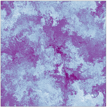
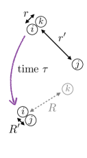
Figure 1: Left: Distance traveled by fluid elements in a 3D turbulent flow during one large-eddy turnover time. Long (white) and short (purple) distances, represented here as a function of the final position in a 2D slice, define an intricate landscape with fronts where particles coming from far apart meet together. Right: Sketch of the event leading to correlated successive collisions. At the initial time (top), two particles $i$ and $k$ are located at a collision distance $r\lesssim\eta$, while a third one $j$ is at distance $r^{\prime}\gg\eta$ far from them. A time $\tau$ later (bottom) $j$ has approached $i$ at a distance $R^{\prime}\lesssim\eta$ while $k$, having collided or not, has escaped to $R\gg\eta$.

In dilute suspensions, a coalescence results from two successive processes. First, the turbulent flow needs to bring two initially separate particles at a sufficiently close distance $\lesssim\eta$. Second, these close particles need to actually merge, and this involves various microphysical mechanisms (particle inertia, hydrodynamical interactions, surface effects). This leads us to write the coalescence rate as a product of two contributions:

$$\lambda_{i,j}(\tau)\approx\lambda_{i,j}^{\rm turb}(\tau)\times\lambda_{i,j}^{\rm micro}.$$ (6)

The contribution from turbulent transport can be written

$$\lambda_{i,j}^{\rm turb}(\tau)\approx\int u_{\eta}\,p_{3}(R,\eta,\tau|\eta,r^{\prime},0)\,({r^{\prime 2}}/{L^{3}})\,\mathrm{d}r^{\prime}\mathrm{d}R$$ (7)

involving the transition probability $p_{3}$ of the three-point motion. More specifically, two successive collisions occur if three particles (see Fig. 1 Right), initially separated by distances $r=\eta$ and an arbitrary $r^{\prime}$, come in a time $\tau$ to distances $R$, arbitrary, and $R^{\prime}=\eta$. The relation (7) is obtained by integrating over all possible initial distances $r^{\prime}$ of the particle from the particle , with a weight $\propto r^{\prime 2}$ given by a uniform three-dimensional spatial distribution. The three tracers , and undergo in a time $\tau$ an evolution from a degenerate triangle with $r\ll r^{\prime}$ to another degenerate triangle with, this time, $R\gg R^{\prime}$. In turbulence, the probability transition between such configurations can be written as

$$p_{3}(R,R^{\prime}\!,\tau|r,r^{\prime}\!,0)\approx\left(\frac{\eta}{r^{\prime}}\right)^{\!2}\!\left(\frac{L}{r^{\prime}}\right)^{\!\!\delta_{3}}\!\!\frac{1}{\varepsilon\tau^{3}}\Psi\!\left(\frac{r^{\prime 2}}{\varepsilon\tau^{3}},\frac{R^{2}}{\varepsilon\tau^{3}}\right)\!,$$

where $\delta_{3}$ is the anomalous part of the scaling exponent associated to the third-order statistics of an advected passive scalar; its value is universal (independent of the injection mechanism) and $\approx 0.18$, as reported from several experimental and numerical studies Warhaft (2000). In the expression above the first factor comes from integration over angles and can be seen as a small solid-angle contribution. The second factor originates from intermittency and gives a dependence upon the integral scale $L$. Physically, it means that when $\delta_{3}>0$, the closer is the third particle, the more likely it is to approach one of the other two. The last terms involve a dimensionless function $\Psi$ that imposes Richardson’s scaling for backward and forward pair evolution. This specific form of the three-point transition probability leads to

$$\lambda_{i,j}^{\rm turb}(\tau) \propto\frac{\nu^{7/4}}{\varepsilon^{1/4}L^{3-\delta_{3}}}\!\int\Psi\!\left(\frac{r^{\prime 2}}{\varepsilon\tau^{3}},\frac{R^{2}}{\varepsilon\tau^{3}}\right)\frac{\mathrm{d}r^{\prime}\mathrm{d}R}{r^{\prime\delta_{3}}\varepsilon\tau^{3}}$$

$$\propto({1}/{\tau_{L}})\left({\tau}/{\tau_{L}}\right)^{-\frac{3}{2}\delta_{3}},$$ (8)

where $\tau_{L}=\varepsilon^{-1/3}L^{2/3}$ is the large-eddy turnover time. Turbulent transport thus leads to a power-law dependence in time of the coalescence rate. Plugging this behavior in the global coalescence rate (2) and by using the population-balance equations (1), one obtains a short-time behavior of the number of particles that reads

$$n_{i}(t)\simeq n_{1}^{i}\left({t}/{\tilde{t}_{i}}\right)^{(1-\frac{3}{2}\delta_{3})(i-2)+1}.$$ (9)

Here the characteristic times $\tilde{t}_{i}$ are $\propto i\,\tau_{L}$, with a proportionality constant that involves the various microphysical rates $\lambda_{j,k}^{\text{micro}}$ of the coalescences leading to . For $\delta_{3}>0$ the algebraic exponent appearing in (9) is smaller than that obtained in (5) from Smoluchowski’s kinetics. The intermittency of turbulence mixing is thus enhancing the short-time growth by coalescence. In addition, the larger is the aggregate size considered, the stronger is this enhancement. Indeed, when $i$ is large and $t\ll i\,\tau_{L}$, the formation of a particle requires a large number of correlated coalescences separated by inertial-range times and the population dynamics is dominated by (9).

In order to corroborate our theoretical predictions on the enhancement of coalescences by turbulent mixing, we have performed direct numerical simulations for the evolution of a dilute population suspended in a turbulent flow. We start from one billion inertial point-particles whose dynamics is given by a viscous Stokes drag:

$$\ddot{\bm{x}}_{n}=-\frac{1}{\tau_{n}}\left[\dot{\bm{x}}_{n}-\bm{u}(\bm{x}_{n},t)\right]\!,$$ (10)

where $\bm{u}$ designates the fluid velocity field. It is obtained numerically by a pseudo-spectral integration of the incompressible Navier–Stokes equation using $2048^{3}$ gridpoints. A large-scale forcing is applied in order to maintain the flow in a developed turbulent state with $\mbox{\it Re}\approx 50\,000$.

The particles follow the flow with a time lag given by their individual response times $\tau_{n}$. Each particle has a virtual radius $a_{n}(t)$ and $\tau_{n}\propto a_{n}^{2}$. We start from a mono-disperse suspension with monomers having initially all the same radius $a_{i}(0)=a_{0}\approx\eta/10$. When two particles approach at a distance equal to the sum of their radii (detected using a billiard algorithm), they merge, conserving mass and momentum. Particles inertia is measured by their Stokes numbers $St_{n}=\tau_{n}\,\varepsilon^{1/2}/\nu^{1/2}$, which is initially small $St_{n}(0)\approx 0.1$. Inertia effects can thus be clearly neglected when interested in inertial-range length or time scales. The suspension is dilute: their volume fraction is approximately $5\times 10^{-5}$, which represents in our flow one particle for each cube of volume $10\,\eta^{3}$ and is consistent with, for example, typical settings in a warm cloud of our atmosphere.

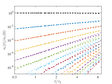
Figure 2: Time evolution of the number $n_{i}(t)$ of particles (normalized by the initial number of monomers $n_{1}(0)$); the mass $i$ increases from 1 to 15 from top to bottom. The dots are the results of direct numerical simulations and the dashed lines show for $i\geq 2$ behaviors $\propto t^{0.73(i-2)+1}$ deduced from (9) for $\delta_{3}=0.18$.

Figure 2 shows on log-log scales the time evolution of the number $n_{i}(t)$ of particles made from the merger of $i$ monomers (that is with radius $a(t)=i^{1/3}a_{0}$) for $i=1,2,\dots 15$. Data (dots) is approximated very well by $n_{i}(t)\propto t^{0.73(i-2)+1}$ (dashed lines), corresponding to the predicted power laws (9) with $\delta_{3}=0.18$. Such a behavior persists for times larger than the large-eddy turnover time. The result of our simulation confirms the accuracy and the relevance of the predictions made earlier in this Letter. Large aggregates are appearing faster than predicted from kinetic models.

To confirm that this enhanced growth is indeed resulting from correlated successive collisions, we have measured the probability density $p_{i,1}(\tau)$ of the time lag $\tau$ between the creation of a particle and its next collision with a . Results are shown in Fig. 3 for $i=2,3,4,5$. The distributions clearly display for $\tau$ in the inertial range a power-law decay, followed by a (stretched) exponential cutoff at $\tau\gtrsim\tau_{L}$. The measured value of the algebraic exponent is consistent with the predicted value $-(3/2)\delta_{3}\approx-0.27$. This confirms that the inter-collision time distribution follows (3) with a time-dependent coalescence rate $\lambda_{i.j}(\tau)\propto\tau^{-\frac{3}{2}\delta_{3}}$.

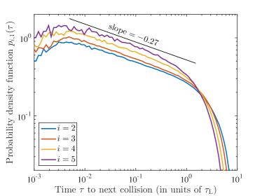
Figure 3: Probability density function of the time between successive coalescences of a particle $i$ with a monomer of mass $1$. The power-law tail has, as we predict theoretically, an exponent $\approx-0.27\approx-({3}/{2})\delta_{3}$

In conclusion, let us stress again that intermittency of turbulent mixing is responsible for an enhanced growth of dilute coalescing aggregates. To our knowledge, this is one of the first instances where turbulent anomalous scaling laws play a critical role in describing to leading order a process with practical implications. Here, only third-order statistics are relevant since successive binary collisions involves the evolution of triplets of tracers that form degenerate triangles. Higher-order statistics enter other configurations (when, for instance, two particles are simultaneously formed and then merge) but they give subleading contributions. Finally, it is worth mentioning that the effect unveiled here might be accounted for by modifying kinetic models. When coarse-graining the population dynamics on sufficiently large timescales, correlated successive collisions will then appear as simultaneous multiple collisions.

The research leading to these results has received funding from the European Research Council under the European Community’s Seventh Framework Program (FP7/2007-2013, Grant Agreement no. 240579), from the Agence Nationale de la Recherche (Programme Blanc ANR-12-BS09-011-04). Access to the IBM BlueGene/P computer JUGENE at the FZ Jülich was made available through the PRACE project PRA031. JB and SSR were supported by the Indo-French Center for Applied Mathematics (IFCAM). SSR acknowledges the AIRBUS Group for the Corporate Foundation Chair in Mathematics of Complex Systems established in ICTS-TIFR.

References

- Weidenschilling and Cuzzi (1993) S. Weidenschilling and J. N. Cuzzi, in Protostars and Planets III, Vol. 1 (1993) pp. 1031–1060.
- Lissauer (1993) J. J. Lissauer, Ann. Rev. Astron. Astrophys. 31, 129 (1993).
- Pinsky and Khain (1997) M. Pinsky and A. Khain, J. Aerosol Sci. 28, 1177 (1997).
- Shaw (2003) R. Shaw, Annu. Rev. Fluid Mech. 35, 183 (2003).
- Wetherill and Stewart (1989) G. Wetherill and G. R. Stewart, Icarus 77, 330 (1989).
- Kostinski and Shaw (2005) A. B. Kostinski and R. A. Shaw, Bull. Am. Met. Soc. 86, 235 (2005).
- Johansen et al. (2015) A. Johansen, M.-M. Mac Low, P. Lacerda, and M. Bizzarro, Science Advances 1, e1500109 (2015).
- Johansen et al. (2007) A. Johansen et al., Nature 448, 1022 (2007).
- Bodenschatz et al. (2010) E. Bodenschatz, S. Malinowski, R. Shaw, and F. Stratmann, Science 327, 970 (2010).
- Sundaram and Collins (1997) S. Sundaram and L. Collins, J. Fluid Mech. 335, 75 (1997).
- Falkovich et al. (2002) G. Falkovich, A. Fouxon, and M. G. Stepanov, Nature 419, 151 (2002).
- Wilkinson et al. (2006) M. Wilkinson, B. Mehlig, and V. Bezuglyy, Phys. Rev. Lett. 97, 048501 (2006).
- Devenish et al. (2012) B. Devenish et al., Q.J.R. Meteorol. Soc. 138, 1401 (2012).
- Pan and Padoan (2014) L. Pan and P. Padoan, Astrophys. J. 797, 101 (2014).
- Bec et al. (2005) J. Bec, A. Celani, M. Cencini, and S. Musacchio, Phys. Fluids 17, 073301 (2005).
- Gustavsson and Mehlig (2013) K. Gustavsson and B. Mehlig, Phys. Rev. E 87, 023016 (2013).
- Voßkuhle et al. (2014) M. Voßkuhle, A. Pumir, E. Lévêque, and M. Wilkinson, J. Fluid Mech. 749, 841 (2014).
- Shraiman and Siggia (2000) B. I. Shraiman and E. D. Siggia, Nature 405, 639 (2000).
- Falkovich et al. (2001) G. Falkovich, K. Gawȩdzki, and M. Vergassola, Rev. Mod. Phys. 73, 913 (2001).
- Smoluchowski (1917) M. Smoluchowski, Zeitschrift f. physik. Chemie 92, 129 (1917).
- Frisch (1995) U. Frisch, Turbulence (Cambridge University Press, Cambridge, England, 1995).
- Falkovich and Sreenivasan (2006) G. Falkovich and K. R. Sreenivasan, Physics Today 59, 43 (2006).
- Arad et al. (2001) I. Arad, L. Biferale, A. Celani, I. Procaccia, and M. Vergassola, Phys. Rev. Lett. 87, 164502 (2001).
- Warhaft (2000) Z. Warhaft, Ann. Rev. Fluid Mech. 32, 203 (2000).