Interior Penalty Mixed Finite Element Methods of Any Order in Any Dimension for Linear Elasticity with Strongly Symmetric Stress Tensor

Abstract

We propose two classes of mixed finite elements for linear elasticity of any order, with interior penalty for nonconforming symmetric stress approximation. One key point of our method is to introduce some appropriate nonconforming face-bubble spaces based on the local decomposition of discrete symmetric tensors, with which the stability can be easily established. We prove the optimal error estimate for both displacement and stress by adding an interior penalty term. The elements are easy to be implemented thanks to the explicit formulations of its basis functions. Moreover, the methods can be applied to arbitrary simplicial grids for any spatial dimension in a unified fashion. Numerical tests for both 2D and 3D are provided to validate our theoretical results.

mmsxxxxxxxx–x

1 Introduction

Mixed finite element methods for linear elasticity are popular methods to approximate the stress-displacement system derived from Hellinger-Reissner variational principle. However, it is more difficult to develop the stable mixed finite element methods for linear elasticity than that for scalar second-order elliptic problems, as the stress tensor is required to be symmetric due to the conservation of angular momentum. One way to circumvent this difficulty is to use composite element techniques [30, 6]. Another approach is to use some well-known $H({\rm div})$ elements to relax the symmetry. One main technique is to introduce a Lagrange multiplier approximating the non-symmetric part of the displacement gradient while enforcing stress symmetry weakly [2, 7, 12, 18, 19, 33, 22].

The first stable non-composite finite element method for classical mixed finite formulation of plane elasticity was proposed by Arnold and Winther in 2002 [8]. In this class of elements, the displacement is discretized by discontinuous piecewise $\mathcal{P}_{k}$ ($k\geq 1$) polynomial, while the stress is discretized by the conforming $\mathcal{P}_{k+2}$ tensors whose divergence is $\mathcal{P}_{k}$ vector on each triangle. The analogue of the results in 3D case were reported in [1, 4]. All the results in this series have some features in common: the degree of polynomial for the displacement should satisfy $k\geq 1$. The similar idea can be applied to the rectangular element, see [3, 17, 25].

Recently Hu and Zhang [27, 28] and Hu [23] proposed a family of conforming mixed elements for $\mathbb{R}^{n}$ that have fewer degrees of freedom than those in the earlier literature. For $k\geq n$, this class of elements are optimal in the sense that the displacement is discretized by discontinuous piecewise $\mathcal{P}_{k}$ polynomial, while the stress is discretized by the conforming $\mathcal{P}_{k+1}$ tensors. These elements also admit a unified theory and a relatively easy implementation. For the case that $k\leq n-1$, the symmetric tensor spaces are enriched by proper high order $H({\rm div})$ bubble functions to stabilize the discretization [29]. Similar mixed elements on rectangular and cuboid grids were constructed in [24].

There have been also numerous works in the literature on nonconforming mixed elements. For rectangular or cuboid grids, we refer to [35, 36, 26, 10, 32]. For simplicial grids, we first refer Arnold and Winther [9] (2D) and [5] (3D). These elements contain the displacement space with $k=1$, but it is suboptimal as only the first order accuracy can be proved for the displacement. In [21], Gopalakrishnan and Guzmán developed a family of simplicial elements for $k\geq 1$ in both two and three dimensions. The optimal convergence order for the displacement can be proved under the full elliptic regularity assumption but the convergence order of $L^{2}$ error for stress is still suboptimal.

All the aforementioned simplicial elements have the constraint that $k\geq 1$. For the lowest order case $k=0$ in 2D, Cai and Ye [15] used the Crouzeix-Raviart element to approximate each component of the symmetric stress and piecewise constants for the displacement. Their method was proved to be convergent by adding an interior penalty term to weakly enforce the continuity of the stress. As the authors claimed, their elements can be extended to higher spatial dimensions, but it is not clear how the elements can be extended to higher orders.

The purpose of this paper is to construct a family of mixed finite elements ($k\geq 0$) for simplicial grids in any dimension. Precisely, the piecewise $\mathcal{P}_{k}$ vector space without interelement continuity is applied to approximate the displacement. To design the piecewise $\mathcal{P}_{k+1}$ spaces for the stress, the crucial point is to introduce the conforming div-bubble spaces [23] and nonconforming face-bubble spaces, with which the stability can easily be established. We then add the spaces with two classes of spaces to obtain the desired approximation property. The first class is locally defined with elementwise degrees of freedom, while the second class does not have local d.o.f. but has a very small dimension. Any space between these two classes can be proved to be convergent. Especially, the finite element space proposed in [15] in lowest order lies in this case. Moreover, our first class of space is precisely the space proposed in [21] when $k\geq 1$, while the d.o.f are slightly different.

Due to the discontinuity of the normal stress on each interior face, the stress-displacement mixed formulation is modified by adding an interior penalty term to weakly enforce the continuity, which is a standard technique for discontinuous Galerkin methods and also adopted in [15]. The convergence of our mixed finite element method is studied according to the three ingredients step by step: stability, approximation and consistency, with which a constructive proof can be obtained naturally. More importantly, based on our knowledge, our second class of spaces in lowest order has the smallest dimension among all the mixed finite elements on simplicial grids regardless whether the symmetry of stress is imposed strongly or weakly.

The rest of the paper is organized as follows. In the next section, we present the local decomposition of discrete symmetric tensors. In section 3, we define two classes of finite element spaces for symmetric tensors in any space dimension from the perspectives of both stability and approximation property. In section 4, the interior penalty mixed finite element method is proposed, and its well-posedness and error analysis are given subsequently. We then discuss the reduced elements in section 5 and prove that the nonconforming elements have to be applied in our framework when $k\leq n-1$. Numerical tests in both 2D and 3D case will be given in section 6 and the concluding remarks will then arrive to close the main text.

2 Local Decomposition of Discrete Symmetric Tensors

In this paper, we consider the following linear elasticity problem with Dirichlet boundary condition

(1) $$\left\{\begin{aligned} \mathcal{A}\boldsymbol{\sigma}-\boldsymbol{\epsilon}(u)&=0\qquad\text{in~{}}\Omega,\\ {\rm div}\boldsymbol{\sigma}&=f\qquad\text{in~{}}\Omega,\\ u&=0\qquad\text{on~{}}\partial\Omega,\end{aligned}\right.$$

where $\Omega\subset\mathbb{R}^{n}$. The displacement and stress are denoted by $u:\Omega\mapsto\mathbb{R}^{n}$ and $\boldsymbol{\sigma}:\Omega\mapsto\mathbb{S}$, respectively. Here, $\mathbb{S}$ represents the space of real symmetric matrices of order $n\times n$. The compliance tensor $\mathcal{A}:\mathbb{S}\mapsto\mathbb{S}$ is assumed to be bounded and symmetric positive definite. The linearized strain tensor is denoted by $\boldsymbol{\epsilon}(u)=(\nabla u+(\nabla u)^{T})/2$.

The mixed formulation of (1) is to find $(\boldsymbol{\sigma},u)\in\Sigma\times V:=H({\rm div},\Omega;\mathbb{S})\times L^{2}(\Omega;\mathbb{R}^{n})$, such that

(2) $$\left\{\begin{aligned} &(\mathcal{A}\boldsymbol{\sigma},\boldsymbol{\tau})_{\Omega}+({\rm div}\boldsymbol{\tau},u)_{\Omega}&=&~{}0\quad&\forall\boldsymbol{\tau}\in\Sigma,\\ &({\rm div}\boldsymbol{\sigma},v)_{\Omega}&=&~{}(f,v)_{\Omega}\quad&\forall v\in V.\end{aligned}\right.$$

Here $H({\rm div},\Omega;\mathbb{S})$ consists of square-integrable symmetric matrix fields with square-integrable divergence. The corresponding $H({\rm div})$ norm is defined by

$$\|\boldsymbol{\tau}\|_{{\rm div},\Omega}^{2}:=\|\boldsymbol{\tau}\|_{0,\Omega}^{2}+\|{\rm div}\boldsymbol{\tau}\|_{0,\Omega}^{2},\quad\forall\boldsymbol{\tau}\in H({\rm div},\Omega;\mathbb{S}).$$

The $L^{2}(\Omega;\mathbb{R}^{n})$ is the space of vector-valued functions which are square-integrable with the standard $L^{2}$ norm.

Throughout this paper, we shall use letter $C$ to denote a generic positive constant independent of $h$ which may stand for different values at its different occurrences. The notation $x\lesssim y$ means $x\leq Cy$ and $x\simeq y$ means $x\lesssim y\lesssim x$.

2.1 Preliminaries

Suppose that the domain $\Omega$ is subdivided by a family of shape regular simplicial grids $\mathcal{T}_{h}=\{K\}$. Let $h_{K}$ be the diameter of element $K$, $h=\max_{K}h_{K}$ be the mesh diameter of $\mathcal{T}_{h}$. The set of all faces of $\mathcal{T}_{h}$ is denoted by $\mathcal{F}_{h}=\{F\}$ with the diameter $h_{F}$ for face $F$. The set of faces can be divided into two parts: the boundary faces set $\mathcal{F}_{h}^{\partial}=\mathcal{F}_{h}\cap\partial\Omega$, and the interior faces set $\mathcal{F}_{h}^{i}=\mathcal{F}_{h}\setminus\mathcal{F}_{h}^{\partial}$. For any $F\in\mathcal{F}_{h}$, the set of all elements that share the face $F$ is denoted by $\mathcal{T}_{h,F}$. The unit normal vector with respect the face $F$ is represented by $\nu_{F}$.

Let $F\in\mathcal{F}_{h}^{i}$ be the common face of two elements $K^{+}$ and $K^{-}$, and $\nu_{F}^{+}$ and $\nu_{F}^{-}$ be the unit outward normal vectors on $F$ with respect to $K^{+}$ and $K^{-}$, respectively. Then we define the jump $[\cdot]$ on $F\in\mathcal{F}_{h}^{i}$ for $\boldsymbol{\tau}:\Omega\mapsto\mathbb{S}$ by

(3) $$[\boldsymbol{\tau}]:=\boldsymbol{\tau}^{+}\nu_{F}^{+}+\boldsymbol{\tau}^{-}\nu_{F}^{-}.$$

For a given simplex $K$, its vertices are denoted by $a_{1},\cdots,a_{n+1}$. The face that does not contain the vertex $a_{i}$ is denoted by $F_{i}$. The barycentric coordinates with respect to $K$ are represented by $\lambda_{1}(x),\cdots,\lambda_{n+1}(x)$. For any edge $e_{ij}=a_{j}-a_{i}$ of element $K$, $i\neq j$, let $t_{ij}$ be the unit tangent vectors along this edge, namely

$$t_{ij}:=\frac{a_{j}-a_{i}}{|a_{j}-a_{i}|}=\frac{a_{j}-a_{i}}{|e_{ij}|}.$$

Then we have the following important result describing the relationship between the simplex $K$ and $\mathbb{S}$.

Lemma 1.

The symmetric tensors $\{t_{ij}t_{ij}^{T},~{}\forall i<j\}$ form a basis of $\mathbb{S}$.

Proof.

See Lemma 2.1 in [23]. ∎

These symmetric matrices $t_{ij}t_{ij}^{T}$ of rank one are the basis ingredients when constructing the finite elements for the symmetric stress tensors. One of the most commonly used properties of these basis functions is

(4) $$t_{ij}t_{ij}^{T}\nu_{F_{s}}=0\iff\forall s\neq i,j.$$

When applying the standard $\mathcal{P}_{k+1}$ Lagrangian element for each entry of the symmetric tensors, we obtain the following $\mathcal{P}_{k+1}(\mathbb{S})$ Lagrangian element:

(5) $$\Sigma_{k+1,h}^{c}:=\{\boldsymbol{\tau}\in H^{1}(\Omega;\mathbb{S})~{}|~{}\boldsymbol{\tau}|_{K}\in\mathcal{P}_{k+1}(K;\mathbb{S})\}.$$

Collect all the face-bubble functions in $\Sigma_{k+1,h}^{c}$, we have the following $H^{1}(\mathbb{S})$ face-bubble function space

(6) $$\Sigma_{k+1,h,f}^{c}:=\left\{\boldsymbol{\tau}\in H^{1}(\Omega;\mathbb{S})~{}|~{}\boldsymbol{\tau}|_{K}\in\sum_{i=1}^{n+1}(\prod_{j=1,j\neq i}^{n+1}\lambda_{j})\mathcal{P}_{k+1-n}(K;\mathbb{S})\right\}.$$

Here we define $\mathcal{P}_{m}(K)=\{0\}$ if $m<0$. Clearly, the $H^{1}(\mathbb{S})$ face-bubble function space is nonempty only when $k\geq n-1$.

2.2 Local decomposition of polynomial spaces

In this subsection, we introduce some polynomial spaces and discuss their relationships.

2.2.1 Some polynomial spaces in simplex $K$

We first give the following lemma that simplifies the reader’s understanding.

Lemma 2.

Suppose $\{\psi_{0},\cdots,\psi_{q}\}(q\geq 0)$ are linearly independent, and $\{\psi_{l}^{k},k=0,1,\cdots\}$ are independent for $1\leq l\leq q$. Then for any $k\geq 0$,

$$\left\{\prod_{l=0}^{q}\psi_{l}^{m_{l}},\sum_{l=0}^{q}m_{l}=k\right\}\text{~{}are linearly independent functions}.$$

Let $\lambda_{0}=1$. For a $n$-dimensional simplex $K$, it is well-known that $\{\lambda_{l},l=0,1,\cdots,n+1\}$ is a set of linearly dependent functions, which forms a basis of $\mathcal{P}_{1}(K;\mathbb{R})$ if any one of them is removed. In light of Lemma 2, $\mathcal{P}_{k}(K;\mathbb{R})$ can be written as

$$\mathcal{P}_{k}(K;\mathbb{R})=\text{span}\left\{\prod_{l=1}^{n+1}\lambda_{l}^{m_{l}},\sum_{l=1}^{n+1}m_{l}=k\right\},$$

or for $i\geq 1$,

$$\mathcal{P}_{k}(K;\mathbb{R})=\text{span}\left\{\prod_{l=0,l\neq i}^{n+1}\lambda_{l}^{m_{l}},\sum_{l=0,l\neq i}^{n+1}m_{l}=k\right\}=\text{span}\left\{\prod_{l=1,l\neq i}^{n+1}\lambda_{l}^{m_{l}},\sum_{l=1,l\neq i}^{n+1}m_{l}\leq k\right\}.$$

Now we introduce the spaces by removing two functions in $\{\lambda_{l},l=0,1,\cdots,n+1\}$. If $\lambda_{0}$ and $\lambda_{i}(1\leq i\leq n)$ are removed, we have the following space

(7) $$\mathcal{P}_{k}^{\hat{0},\hat{i}}(K;\mathbb{R}):=\text{span}\left\{\prod_{l=1,l\neq i}^{n+1}\lambda_{l}^{m_{l}},\sum_{l=1,l\neq i}^{n+1}m_{l}=k\right\}.$$

If $\lambda_{i},\lambda_{j}(1\leq i\neq j\leq n)$ are removed, we have

(8) $$\mathcal{P}_{k}^{\hat{i},\hat{j}}(K;\mathbb{R}):=\text{span}\left\{\prod_{l=0,l\neq i,j}^{n+1}\lambda_{l}^{m_{l}},\sum_{l=0,l\neq i,j}^{n+1}m_{l}=k\right\}=\text{span}\left\{\prod_{l=1,l\neq i,j}^{n+1}\lambda_{l}^{m_{l}},\sum_{l=1,l\neq i,j}^{n+1}m_{l}\leq k\right\}.$$

2.2.2 Natural restriction and extension operators

The restriction operator is defined as

(9) $$\mathcal{R}_{i}:\mathcal{P}_{k}(K;\mathbb{R})\mapsto\mathcal{P}_{k}(F_{i};\mathbb{R}),\quad\mathcal{R}_{i}p:=p|_{F_{i}},\quad\forall p\in\mathcal{P}_{k}(K;\mathbb{R}).$$

For any $F_{i}\subset\partial K$, we have $\lambda_{i}|_{F_{i}}=0$ and for $l\neq i$, $\lambda_{l}^{F_{i}}=\lambda_{l}|_{F_{i}}$ are exactly the barycentric coordinates on $F_{i}$. For any $p\in\mathcal{P}_{k}(F_{i};\mathbb{R})$, it can be uniquely written under the basis $\{\lambda_{l}^{F_{i}},l\neq i,j\}$, i.e.

$$p=\sum_{|\boldsymbol{m}|=k}c_{\boldsymbol{m}}\prod_{l=0,l\neq i,j}^{n+1}\lambda_{l}^{F_{i},m_{l}}.$$

Then the extension operator is denoted as

(10) $$\mathcal{E}_{i}^{\hat{j}}:\mathcal{P}_{k}(F_{i};\mathbb{R}) \mapsto\mathcal{P}_{k}(K;\mathbb{R})\qquad 0\leq j\neq i\leq n+1,$$

$$\mathcal{E}_{i}^{\hat{j}}p :=\sum_{|\boldsymbol{m}|=k}c_{\boldsymbol{m}}\prod_{l=0,l\neq i,j}^{n+1}\lambda_{l}^{m_{l}}.$$

With the help of $\mathcal{R}_{i}$ and $\mathcal{E}_{i}^{\hat{j}}$, we have the following properties:

Lemma 3.

It holds that

1. $\mathcal{R}_{i}\mathcal{E}_{i}^{\hat{j}}=id_{\mathcal{P}_{k}(F_{i};\mathbb{R})},~{}\forall j\neq i$.

2. $\ker(\mathcal{R}_{i})\cap\mathcal{P}_{k}(K;\mathbb{R})=\lambda_{i}\mathcal{P}_{k-1}(K;\mathbb{R})$.

3. $\mathcal{P}_{k}^{\hat{0},\hat{i}}(K;\mathbb{R})=\mathrm{range}(\mathcal{E}_{i}^{\hat{0}}),\quad\mathcal{P}_{k}^{\hat{i},\hat{j}}(K;\mathbb{R})=\mathrm{range}(\mathcal{E}_{i}^{\hat{j}})=\mathrm{range}(\mathcal{E}_{j}^{\hat{i}})$.

4. $\mathcal{P}_{k}^{\hat{0},\hat{i}}(K;\mathbb{R})\cong\mathcal{P}_{k}(F_{i};\mathbb{R}),~{}\forall 1\leq i\leq n+1$.

5. $\mathcal{P}_{k}^{\hat{i},\hat{j}}(K;\mathbb{R})|_{F_{i}}\cong\mathcal{P}_{k}(F_{i};\mathbb{R}),~{}\mathcal{P}_{k}^{\hat{i},\hat{j}}(K;\mathbb{R})|_{F_{j}}\cong\mathcal{P}_{k}(F_{j};\mathbb{R}),~{}\forall 1\leq i<j\leq n+1$.

6. $\lambda_{i}\mathcal{P}_{k}^{\hat{0},\hat{j}}(K;\mathbb{R})\cap\lambda_{j}\mathcal{P}_{k}^{\hat{0},\hat{i}}(K;\mathbb{R})=\{0\},~{}\forall 1\leq i\neq j\leq n+1$.

Proof.

The properties 1-5 are derived from the definition of natural restriction and extension operators. For any $p\in\lambda_{i}\mathcal{P}_{k}^{\hat{0},\hat{j}}(K;\mathbb{R})\cap\lambda_{j}\mathcal{P}_{k}^{\hat{0},\hat{i}}(K;\mathbb{R})$, we immediately have $\mathcal{R}_{i}p=0$ and $p=\lambda_{j}\mathcal{E}_{i}^{\hat{0}}q$, where $q\in\mathcal{P}_{k}(F_{i};\mathbb{R})$. Then

$$0=\mathcal{R}_{i}p=\lambda_{j}^{F_{i}}\mathcal{R}_{i}\mathcal{E}_{i}^{\hat{0}}q=\lambda_{j}^{F_{i}}q,$$

which implies $q=0$ thus $p=0$. ∎

Without loss of clarity in what follows, we will use same notation $\lambda_{l}$ for barycentric coordinates of both $K$ and $F$.

2.2.3 Local Decomposition of $\mathcal{P}_{k+1}(K;\mathbb{R})$

We first give the following lemma.

Lemma 4.

Let $\tilde{\mathcal{R}}:V\mapsto W$ and $\tilde{\mathcal{E}}:W\mapsto V$ be bounded linear operators between Banach spaces. If $\tilde{\mathcal{X}}=\tilde{\mathcal{R}}\tilde{\mathcal{E}}$ is an isomorphism on $W$, then

(11) $$V=\ker(\tilde{\mathcal{R}})\oplus\mathrm{range}(\mathcal{\tilde{E}}).$$

Remark 5.

Take $\tilde{\mathcal{R}}=\mathcal{R}_{i}$ and $\tilde{\mathcal{E}}=\mathcal{E}_{i}^{\hat{j}}$ in Lemma 4, we immediately have

(12) $$\mathcal{P}_{k}(K;\mathbb{R})=\lambda_{i}\mathcal{P}_{k-1}(K;\mathbb{R})\oplus\mathcal{P}_{k}^{\hat{i},\hat{j}}(K;\mathbb{R})\qquad 0\leq j\neq i\leq n+1.$$

Let $\mathcal{P}_{k}^{\perp}(F_{j};\mathbb{R})\subset\mathcal{P}_{k+1}(F_{j};\mathbb{R})$ be the $L^{2}$ orthogonal complement $\mathcal{P}_{k}(F_{j};\mathbb{R})$ in $\mathcal{P}_{k+1}(F_{j};\mathbb{R})$, namely for $1\leq j\leq n+1$,

$$\mathcal{P}_{k+1}(F_{j};\mathbb{R}) =\Pi_{k,F_{j}}^{0}\mathcal{P}_{k+1}(F_{j};\mathbb{R})\oplus(I-\Pi_{k,F_{j}}^{0})\mathcal{P}_{k+1}(F_{j};\mathbb{R})$$

$$=\mathcal{P}_{k}(F_{j};\mathbb{R})\oplus\mathcal{P}_{k}^{\perp}(F_{j};\mathbb{R}),$$

where $\Pi_{k,F_{j}}^{0}$ is the $L^{2}$ projection operator to $\mathcal{P}_{k}(F_{j};\mathbb{R})$. Now we present the local decomposition of $\mathcal{P}_{k+1}(K;\mathbb{R})$ as follows.

Theorem 6.

For any given $1\leq i<j\leq n+1$, it holds that

(13) $$\mathcal{P}_{k+1}(K;\mathbb{R})=\lambda_{i}\lambda_{j}\mathcal{P}_{k-1}(K;\mathbb{R}) \oplus\lambda_{j}\mathcal{E}_{i}^{\hat{0}}\mathcal{P}_{k}(F_{i};\mathbb{R})$$

$$\oplus\lambda_{i}\mathcal{E}_{j}^{\hat{0}}\mathcal{P}_{k}(F_{j};\mathbb{R})\oplus\mathcal{E}_{j}^{\hat{i}}\mathcal{P}_{k}^{\perp}(F_{j};\mathbb{R}).$$

Proof.

Take $\tilde{\mathcal{R}}=\mathcal{R}_{j}$, $\tilde{\mathcal{E}}=\lambda_{i}\mathcal{E}_{j}^{\hat{0}}\Pi_{k,F_{j}}^{0}+\mathcal{E}_{j}^{\hat{i}}(I-\Pi_{k,F_{j}}^{0})$ in Lemma 4. A simple calculation shows that $\tilde{\mathcal{X}}=\tilde{\mathcal{R}}\tilde{\mathcal{E}}:\mathcal{P}_{k+1}(F_{j};\mathbb{R})\mapsto\mathcal{P}_{k+1}(F_{j};\mathbb{R})$. Since $\dim(\mathcal{P}_{k+1}(F_{j};\mathbb{R}))<\infty$, we only need to check that $\tilde{\mathcal{X}}$ is one-to-one to prove it isomorphism. For any $p_{j}\in\ker(\tilde{\mathcal{X}})$, we have

$$0=\tilde{\mathcal{X}}p_{j}=\mathcal{R}_{j}\lambda_{i}\mathcal{E}_{j}^{\hat{0}}\Pi_{k,F_{j}}^{0}p_{j}+\mathcal{R}_{j}\mathcal{E}_{j}^{\hat{i}}(I-\Pi_{k,F_{j}}^{0})p_{j}=\lambda_{i}\Pi_{k,F_{j}}^{0}p_{j}+(I-\Pi_{k,F_{j}}^{0})p_{j}.$$

Apply $\Pi_{k,F_{j}}^{0}$ on both sides, we have

$$\Pi_{k,F_{j}}^{0}\left(\lambda_{i}\Pi_{k,F_{j}}^{0}p_{j}\right)=0\quad\text{or}\quad\int_{F_{j}}\lambda_{i}\Pi_{k,F_{j}}^{0}p_{j}q=0,~{}\forall q\in\mathcal{P}_{k}(F_{j};\mathbb{R}),$$

which implies $\Pi_{k,F_{j}}^{0}p_{j}=0$ by taking $q=\Pi_{k,F_{j}}p_{j}$. Then $(I-\Pi_{k,F_{j}}^{0})p_{j}=0$ thus $p_{j}=0$.

In light of Lemma 4, we have

(14) $$\mathcal{P}_{k+1}(K;\mathbb{R})=\ker(\mathcal{R}_{j})\oplus\mathrm{range}(\mathcal{\tilde{E}}).$$

From Lemma 3 and (12),

(15) $$\ker(\mathcal{R}_{j})\cap\mathcal{P}_{k+1}(K;\mathbb{R})=\lambda_{j}\mathcal{P}_{k}(K;\mathbb{R}) =\lambda_{j}\left(\lambda_{i}\mathcal{P}_{k-1}(K;\mathbb{R})\oplus\mathcal{E}_{i}^{\hat{0}}\mathcal{P}_{k}(F_{i};\mathbb{R})\right)$$

$$=\lambda_{i}\lambda_{j}\mathcal{P}_{k-1}(K;\mathbb{R})\oplus\lambda_{j}\mathcal{E}_{i}^{\hat{0}}\mathcal{P}_{k}(F_{i};\mathbb{R}).$$

And

(16) $$\mathrm{range}(\tilde{\mathcal{E}})=\lambda_{i}\mathcal{E}_{j}^{\hat{0}}\mathcal{P}_{k}(F_{j};\mathbb{R})+\mathcal{E}_{j}^{\hat{i}}\mathcal{P}_{k}^{\perp}(F_{j};\mathbb{R}).$$

If $p\in\lambda_{i}\mathcal{E}_{j}^{\hat{0}}\mathcal{P}_{k}(F_{j};\mathbb{R})\cap\mathcal{E}_{j}^{\hat{i}}\mathcal{P}_{k}^{\perp}(F_{j};\mathbb{R})$, then $\mathcal{R}_{j}p\in\lambda_{i}\mathcal{P}_{k}(F_{j};\mathbb{R})\cap\mathcal{P}_{k}^{\perp}(F_{j};\mathbb{R})=\{0\}$, which implies $p\in\ker(\mathcal{R}_{j})$. Then we have $p=0$ in light of (14), which means the sum in (16) is direct. Take (15) and (16) into (14), we obtain the local decomposition (13). ∎

For the last term in (13), we will show its symmetry with respect to $i$ and $j$.

Lemma 7.

It holds that

(17) $$\mathcal{E}_{j}^{\hat{i}}\mathcal{P}_{k}^{\perp}(F_{j};\mathbb{R})=\mathcal{E}_{i}^{\hat{j}}\mathcal{P}_{k}^{\perp}(F_{i};\mathbb{R}).$$

Proof.

Note that $\mathcal{E}_{j}^{\hat{i}}\mathcal{P}_{k}(F_{j};\mathbb{R})=\mathcal{E}_{i}^{\hat{j}}\mathcal{P}_{k}(F_{i};\mathbb{R})$, then for any $p\in\mathcal{E}_{i}^{\hat{j}}\mathcal{P}_{k}^{\perp}(F_{i};\mathbb{R})$ and $q_{j}\in\mathcal{P}_{k}(F_{j};\mathbb{R})$, there exists $p_{j}\in\mathcal{P}_{k+1}(F_{j};\mathbb{R})$ and $q_{i}\in\mathcal{P}_{k}(F_{i};\mathbb{R})$, such that

$$p=\mathcal{E}_{j}^{\hat{i}}p_{j},\qquad q_{i}=\mathcal{R}_{i}\mathcal{E}_{j}^{\hat{i}}q_{j}.$$

Hence, $p\in\mathcal{E}_{i}^{\hat{j}}\mathcal{P}_{k}^{\perp}(F_{i};\mathbb{R})$ implies that

(18) $$\int_{F_{i}}\mathcal{R}_{i}\mathcal{E}_{j}^{\hat{i}}p_{j}\cdot\mathcal{R}_{i}\mathcal{E}_{j}^{\hat{i}}q_{j}\mathrm{d}x=0.$$

Define the affine mapping $A^{i,j}:F_{i}\mapsto F_{j}$ by

$$A^{i,j}(a_{s})=a_{s},s\neq i,j\quad\text{and}\quad A^{i,j}(a_{i})=a_{j}.$$

It is straightforward that

$$\lambda_{s}^{F_{i}}(x)=\lambda_{s}^{F_{j}}(A^{i,j}(x)),s\neq i,j\quad\text{and}\quad\lambda_{j}^{F_{i}}(x)=\lambda_{i}^{F_{j}}(A^{i,j}(x)),$$

and

$$(\mathcal{R}_{i}\mathcal{E}_{j}^{\hat{i}}f_{j})(x)=f_{j}(A^{i,j}(x))\qquad\forall f_{j}\in\mathcal{P}_{k}(F_{j};\mathbb{R}).$$

Then (18) implies

$$0=\int_{F_{i}}p_{j}(A^{i,j}(x))\cdot q_{j}(A^{i,j}(x))\mathrm{d}x=\det(DA^{i,j})^{-1}\int_{F_{j}}p_{j}(y)q_{j}(y)\mathrm{d}y,$$

where $DA^{i,j}$ is the Jaboci of $A^{i,j}$. Then $p_{j}\in\mathcal{P}_{k}^{\perp}(F_{j};\mathbb{R})$ thus $p\in\mathcal{E}_{j}^{\hat{i}}\mathcal{P}_{k}^{\perp}(F_{j};\mathbb{R})$. Therefore, $\mathcal{E}_{i}^{\hat{j}}\mathcal{P}_{k}^{\perp}(F_{j};\mathbb{R})\subset\mathcal{E}_{j}^{\hat{i}}\mathcal{P}_{k}^{\perp}(F_{i};\mathbb{R})$. ∎

2.3 Local decomposition of $\mathcal{P}_{k+1}(K;\mathbb{S})$

In light of Theorem 6 and Lemma 1, we immediately have the local decomposition of $\mathcal{P}_{k+1}(K;\mathbb{S})$ as

(19) $$\mathcal{P}_{k+1}(K;\mathbb{S})=\bigoplus_{1\leq i<j\leq n+1}\Big{(}\lambda_{i}\lambda_{j}\mathcal{P}_{k-1}(K;\mathbb{R}) \oplus\lambda_{j}\mathcal{P}_{k}^{\hat{0},\hat{i}}(K;\mathbb{R})$$

$$\oplus\lambda_{i}\mathcal{P}_{k}^{\hat{0},\hat{j}}(K;\mathbb{R})\oplus\mathcal{E}_{j}^{\hat{i}}\mathcal{P}_{k}^{\perp}(F_{j};\mathbb{R})\Big{)}t_{ij}t_{ij}^{T}.$$

Therefore, we can define the following three spaces:

1. local conforming div-bubble function spaces (see also [23])

   (20) $$\Sigma_{k+1,h,b}(K):=\bigoplus_{1\leq i<j\leq n+1}\lambda_{i}\lambda_{j}\mathcal{P}_{k-1}(K;\mathbb{R})t_{ij}t_{ij}^{T}.$$

2. local face-bubble function spaces

   (21) $$\tilde{\Sigma}_{k+1,h,f}(K) :=\bigoplus_{1\leq i<j\leq n+1}\left(\lambda_{i}\mathcal{P}_{k}^{\hat{0},\hat{j}}(K;\mathbb{R})\oplus\lambda_{j}\mathcal{P}_{k}^{\hat{0},\hat{i}}(K;\mathbb{R})\right)t_{ij}t_{ij}^{T},$$

   $$:=\bigoplus_{i=1}^{n+1}\tilde{\Sigma}_{k+1,h,F_{i}}(K),$$

   where

   (22) $$\tilde{\Sigma}_{k+1,h,F_{i}}(K):=\bigoplus_{j=1,j\neq i}^{n+1}\lambda_{j}\mathcal{P}_{k}^{\hat{0},\hat{i}}(K;\mathbb{R})t_{ij}t_{ij}^{T}.$$

3. local nonconforming div-bubble function spaces

   (23) $$\tilde{\Sigma}_{k+1,h,b}(K):=\bigoplus_{1\leq i<j\leq n+1}\mathcal{E}_{j}^{\hat{i}}\mathcal{P}_{k}^{\perp}(F_{j};\mathbb{R})t_{ij}t_{ij}^{T}.$$

The following local decomposition of $\mathcal{P}_{k+1}(K;\mathbb{S})$ then follows from the definition of spaces and (19) directly.

Theorem 8.

It holds that

(24) $$\mathcal{P}_{k+1}(K;\mathbb{S})=\Sigma_{k+1,h,b}(K)\oplus\tilde{\Sigma}_{k+1,h,f}(K)\oplus\tilde{\Sigma}_{k+1,h,b}(K).$$

2.4 Unisolvent set of degrees of freedom for local face-bubble function spaces

From (22) and Lemma 3, we have

$$\tilde{\Sigma}_{k+1,h,F_{i}}(K)\nu_{F_{i}}|_{F_{i}} =\sum_{j=1,j\neq i}^{n+1}\lambda_{j}\mathcal{R}_{i}\left(\mathcal{P}_{k}^{\hat{0},\hat{i}}(K;\mathbb{R})\right)t_{ij}(t_{ij}^{T}\nu_{F_{i}})$$

$$=\sum_{j=1,j\neq i}^{n+1}\lambda_{j}\mathcal{P}_{k}(F_{i};\mathbb{R})t_{ij}$$

$$=T^{\hat{i}}D_{\lambda}^{\hat{i}}\mathcal{P}_{k}(F_{i};\mathbb{R}^{n}),$$

where $D_{\lambda}^{\hat{i}}=\mathop{\operator@font diag}\nolimits(\lambda_{1},\cdots,\lambda_{i-1},\lambda_{i+1},\cdots,\lambda_{n+1}),T^{\hat{i}}=(t_{i1},\cdots,t_{i,i-1},t_{i,i+1},\cdots,t_{i,n+1})\in\mathbb{R}^{n\times n}$. It is apparent that $\det(T^{\hat{i}})\neq 0$, and one inner product of $\mathcal{P}_{k}(F_{i};\mathbb{R}^{n})$ can be defined as

(25) $$\langle\cdot,\cdot\rangle_{D_{\lambda}^{\hat{i}}}:=\int_{F_{i}}D_{\lambda}^{\hat{i}}p\cdot q\qquad\forall p,q\in\mathcal{P}_{k}(F_{i};\mathbb{R}^{n}).$$

Therefore, the unisolvent set of d.o.f. for $\tilde{\Sigma}_{k+1,h,F_{i}}(K)$ can be written as

(26) $$N_{F_{i}}^{\mu}(\boldsymbol{\tau}):=\int_{F_{i}}\boldsymbol{\tau}\nu_{F_{i}}\cdot\mu\qquad\forall\mu\in\mathcal{P}_{k}(F_{i};\mathbb{R}^{n}).$$

Basic functions for a specific set of degrees of freedom

Denote $\{\varphi_{F_{i},t},t=1,\cdots,C_{k+n-1}^{k}\}$ as a basis of $\mathcal{P}_{k}(F_{i};\mathbb{R})$. For convenience, $\varphi_{F_{i},t}$ are normalized such that $\frac{1}{|F_{i}|}\int_{F_{i}}\varphi_{F_{i},t}^{2}=1$. Then

$$\mathcal{P}_{k}(F_{i};\mathbb{R}^{n})=\text{span}\left\{\varphi_{F_{i},t}e_{m},~{}t=1,\cdots,C_{k+n-1}^{k},m=1,\cdots,n\right\},$$

where $e_{m}~{}(m=1,\cdots,n)$ are the unit vectors in $\mathbb{R}^{n}$. Hence, the set of d.o.f. defined in (26) is equivalent to

(27) $$N_{F_{i}}^{t,m}(\boldsymbol{\tau}):=\int_{F_{i}}\boldsymbol{\tau}\nu_{F_{i}}\varphi_{F_{i},t}\cdot e_{m}\qquad t=1,\cdots,C_{k+n-1}^{k},~{}m=1,\cdots,n.$$

Theorem 9.

The basis functions for $N_{F_{i}}^{t,m}(\cdot)$ can be written as

(28) $$\boldsymbol{\phi}_{F_{i}}^{s,l}:=\frac{1}{|F_{i}|}\sum_{1\leq j\leq n+1,j\neq i}\frac{\alpha_{ij}^{l}}{t_{ij}\cdot\nu_{F_{i}}}\lambda_{j}\varphi_{j,s}^{\hat{0},\hat{i}}t_{ij}t_{ij}^{T},$$

where $\sum_{1\leq j\leq n+1,j\neq i}\alpha_{ij}^{l}t_{ij}=e_{l}$, and $\varphi_{j,s}^{\hat{0},\hat{i}}\in\mathcal{P}_{k}^{\hat{0},\hat{i}}(K;\mathbb{R})$ are uniquely determined by

(29) $$\langle\varphi^{\hat{0},\hat{i}}_{j,s},\varphi_{F_{i},t}\rangle_{\lambda_{j}}:=\frac{1}{|F_{i}|}\int_{F_{i}}\lambda_{j}\hat{\varphi}_{j,s}^{\hat{0},\hat{i}}\varphi_{F_{i},t}=\delta_{st}\qquad t=1,\cdots,C_{n-1+k}^{k},$$

Proof.

The lemma is followed by

$$N_{F_{i}}^{t,m}(\boldsymbol{\phi}_{F_{i}}^{s,l}) =\left(\int_{F_{i}}\boldsymbol{\phi}_{F_{i}}^{s,l}\nu_{F_{i}}\varphi_{F_{i},t}\right)\cdot e_{m}$$

$$=\frac{1}{|F_{i}|}\left(\sum_{1\leq j\leq n+1,j\neq i}\int_{F_{i}}\alpha_{ij}^{l}\lambda_{j}\varphi_{j,s}^{\hat{0},\hat{i}}\varphi_{F_{i},t}t_{ij}\right)\cdot e_{m}$$

$$=\delta_{st}\left(\sum_{1\leq j\leq n+1,j\neq i}\alpha_{ij}^{l}t_{ij}\right)\cdot e_{m}=\delta_{st}\delta_{lm}.$$

∎

We can have the explicit formulation of the coefficient $\alpha_{ij}^{l}$ in (28) as follows.

Lemma 10.

Given $i$, for any vector $v$, we have

(30) $$v=\sum_{1\leq j\leq n+1,j\neq i}v\cdot(\nabla\lambda_{j})|e_{ij}|t_{ij}.$$

Proof.

For $u_{h}\in\mathcal{P}_{1}(K)$, we write $u_{h}=\sum_{i=j}^{n+1}u_{j}\lambda_{j}$. Let $\xi=\nabla u_{h}\in\mathbb{R}^{n}$. Then,

$$|K|v\cdot\xi =(v,\nabla u_{h})_{K}=\sum_{j=1}^{n+1}(v,\nabla\lambda_{j})_{K}u_{j}=\sum_{1\leq j\leq n+1,j\neq i}(v,\nabla\lambda_{j})_{K}(u_{j}-u_{i})$$

$$=\sum_{1\leq j\leq n+1,j\neq i}(v,\nabla\lambda_{j})_{K}|e_{ij}|t_{ij}\cdot\xi,$$

which implies (30). ∎

In light of Lemma 10, we have

$$\alpha_{ij}^{l}=e_{l}\cdot(\nabla\lambda_{j})|e_{ij}|\quad\text{and}\quad\boldsymbol{\phi}_{F_{i}}^{s,l}=\frac{1}{|F_{i}|}\sum_{1\leq j\leq n+1,j\neq i}\frac{e_{l}\cdot(\nabla\lambda_{j})|e_{ij}|}{t_{ij}\cdot\nu_{F_{i}}}\lambda_{j}\varphi_{j,s}^{\hat{0},\hat{i}}t_{ij}t_{ij}^{T}.$$

Remark 11.

For the lowest case $k=0$, we immediately obtain that $\varphi_{F_{i},1}=1$ and $\varphi_{j,1}^{\hat{0},\hat{i}}=n,\forall i,j$ by (29). Therefore, basis functions (28) have the following formulation

(31) $$\boldsymbol{\phi}_{F_{i}}^{1,l}=\frac{1}{|F_{i}|}\sum_{1\leq j\leq n+1,j\neq i}\frac{ne_{l}\cdot(\nabla\lambda_{j})|e_{ij}|}{t_{ij}\cdot\nu_{F_{i}}}\lambda_{j}t_{ij}t_{ij}^{T}.$$

In light of the formulation of $\boldsymbol{\phi}_{F_{i}}^{s,l}$ in (28), we have the following properties of the face-bubble $\boldsymbol{\phi}_{F_{i}}^{s,l}$ by standard scaling argument.

Lemma 12.

For any $K\in\mathcal{T}_{h}$ and $F_{i}\subset\partial K$, we have

(32a) $$\|\boldsymbol{\phi}_{F_{i}}^{s,l}\|_{0,K} \lesssim h_{K}^{-n/2+1},$$

(32b) $$\|\boldsymbol{\phi}_{F_{i}}^{s,l}\|_{{\rm div},K} \lesssim h_{K}^{-n/2},$$

(32c) $$\|\boldsymbol{\phi}_{F_{i}}^{s,l}\nu_{F_{i}}\|_{0,F_{i}} \lesssim h_{K}^{-(n-1)/2}.$$

3 Stability and Approximation Property

For the discretization of displacement, the most natural space is the full $C^{-1}-\mathcal{P}_{k}$ space

(33) $$V_{k,h}:=\{v\in L^{2}(\Omega;\mathbb{R}^{n})~{}|~{}v|_{K}\in\mathcal{P}_{k}(K;\mathbb{R}^{n})\}.$$

For the discretization of symmetric stress, we try to find some good approximation spaces under the constrain that the degree of polynomials are at most $k+1$. To this end, we will discuss the effects of different components in the local decomposition (24).

3.1 Stability for $R_{k}^{\perp}$: conforming div-bubble function spaces

Combine the local conforming ${\rm div}$-bubble functions in (20) element by element, we obtain the conforming ${\rm div}$-bubble function spaces

(34) $$\Sigma_{k+1,h,b}:=\{\boldsymbol{\tau}~{}|~{}\boldsymbol{\tau}|_{K}\in\Sigma_{k+1,h,b}(K),~{}\forall K\in\mathcal{T}_{h}\},$$

which satisfies the $\boldsymbol{\tau}\nu_{F}=0$ for any $F\in\mathcal{F}_{h}$. Hu [23] also proved that $\Sigma_{k+1,h,b}$ are exactly the full $H({\rm div};\mathbb{S})$ bubble function spaces. We note that the conforming ${\rm div}$-bubble spaces are non-trivial when the degrees of stress tensor spaces are quadratic at least ($k+1\geq 2$). $\Sigma_{k+1,h,b}$ was introduced in [23] to control the orthogonal complement of the rigid motion space. Precisely, let

(35) $$R_{k}(K) :=\{v\in\mathcal{P}_{k}(K;\mathbb{R}^{n})~{}|~{}(\nabla v+\nabla v^{T})/2=0\},$$

$$R_{k} :=\{v\in V_{k,h}~{}|~{}v|_{K}\in R_{k}(K),~{}\forall K\in\mathcal{T}_{h}\},$$

and

(36) $$R^{\perp}_{k}(K) :=\{v\in\mathcal{P}_{k}(K;\mathbb{R}^{n})~{}|~{}(v,w)_{K}=0\text{~{}for any~{}}w\in R(K)\},$$

$$R^{\perp}_{k} :=\{v\in V_{k,h}~{}|~{}v|_{K}\in R^{\perp}_{k}(K),~{}\forall K\in\mathcal{T}_{h}\}.$$

It is easy to check that $R_{0}=V_{0,h}$, namely the rigid motion space in lowest order is piecewise constant vector space. Together with the higher order case given by Hu [23], we have the following lemma.

Lemma 13.

It holds that

(37) $${\rm div}\Sigma_{k+1,h,b}=R^{\perp}_{k}\qquad\forall k\geq 0.$$

Proof.

The proof is presented here for the completeness. First, (37) is trivially true for $k=0$. Now, we assume $k\geq 1$. The definition of $R_{k}$ implies ${\rm div}\Sigma_{k+1,h,b}\subset R_{k}^{\perp}$. Next we prove that only the zero function $v\in R_{k}^{\perp}(K)$ satisfies

(38) $$\int_{K}{\rm div}\boldsymbol{\tau}\cdot v=-\int_{K}\boldsymbol{\tau}:\boldsymbol{\epsilon}(v)=0\qquad\forall\boldsymbol{\tau}\in\Sigma_{k+1,h,b}(K).$$

By Lemma 1, there exists a basis of $\mathbb{S}$ dual to $\{t_{ij}t_{ij}^{T},1\leq i<j\leq n+1\}$ under the inner product $\langle A,B\rangle:=A:B$, denoted as $\{M_{ij},1\leq i<j\leq n+1\}$. Notice that $\boldsymbol{\epsilon}(v)\in\mathcal{P}_{k-1}(K;\mathbb{S})$, let

$$\boldsymbol{\epsilon}(v)=\sum_{1\leq i<j\leq n+1}q_{ij}M_{ij}\qquad q_{ij}\in\mathcal{P}_{k-1}(\mathbb{R}).$$

Take $\boldsymbol{\tau}=\sum_{1\leq i<j\leq n+1}\lambda_{i}\lambda_{j}q_{ij}t_{ij}t_{ij}^{T}$ in (38) to have

$$0=\sum_{1\leq i<j\leq n+1}\int_{K}\lambda_{i}\lambda_{j}q_{ij}^{2},$$

which implies $q_{ij}=0$, thus $v\in R_{k}(K)\cap R_{k}^{\perp}(K)=0$. ∎

It follows from the definition of $R_{k}$ and $R_{k}^{\perp}$ that $V_{k,h}=R_{k}\oplus R_{k}^{\perp}$. Therefore, for any given $v_{h}\in V_{k,h}$, there uniquely exist $v_{h,R}\in R_{k}$ and $v_{h,R^{\perp}}\in R_{k}^{\perp}$ such that $v_{h}=v_{h,R}+v_{h,R^{\perp}}$. By $L^{2}$ orthogonality,

$$\|v_{h,R}\|_{0}^{2}+\|v_{h,R^{\perp}}\|_{0}^{2}=\|v_{h}\|_{0}^{2}.$$

When constructing the stable pair $\Sigma_{k+1,h}-V_{k,h}$ of mixed finite elements for elasticity, one key step is to find the stable $\boldsymbol{\tau}_{h}\in\Sigma_{k+1,h}$ that ${\rm div}\boldsymbol{\tau}_{h}=v_{h}$. The following lemma implies that the conforming ${\rm div}$-bubble spaces solve the orthogonal complement of the rigid motion.

Lemma 14.

For any $v_{h,R^{\perp}}\in R_{k}^{\perp}(K)$, there exists $\boldsymbol{\tau}_{1}\in\Sigma_{k+1,h,b}(K)$ such that

(39) $${\rm div}\boldsymbol{\tau}_{1}=v_{h,R^{\perp}}\qquad\|\boldsymbol{\tau}_{1}\|_{{\rm div}}\lesssim\|v_{h,R^{\perp}}\|_{0}.$$

Proof.

It follows from Lemma 13 that ${\rm div}:\Sigma_{k+1,h,b}(K)\mapsto R_{k}^{\perp}(K)$ is onto. Then the quotient mapping $\tilde{{\rm div}}:\Sigma_{k+1,h,b}(K)/\ker({\rm div})\mapsto R_{k}^{\perp}(K)$ is isomorphism. Therefore, there uniquely exists $\boldsymbol{\tau}_{1}\in\ker({\rm div})^{\perp}\cap\Sigma_{k+1,h,b}(K)$ such that

$${\rm div}\boldsymbol{\tau}_{1}=v_{h,R^{\perp}}.$$

It then follows from the definition of $\boldsymbol{\tau}_{1}$ and scaling argument that

$$\|\boldsymbol{\tau}_{1}\|_{{\rm div}}\lesssim\|{\rm div}\boldsymbol{\tau}_{1}\|_{0}=\|v_{h,R^{\perp}}\|_{0}.$$

∎

3.2 Stability for $R_{k}$: face-bubble function spaces

In light of Lemma 14, the remaining question for stability is to solve the rigid motion, namely to find the stable $\boldsymbol{\tau}_{2}\in\Sigma_{k+1,h}$ that ${\rm div}_{h}\boldsymbol{\tau}_{2}=v_{h,R}$. Here ${\rm div}_{h}$ is the ${\rm div}$ operator element by element. And the discrete ${\rm div}$ norm is denoted by

$$\|\boldsymbol{\tau}\|_{{\rm div},h}^{2}:=\sum_{K\in\mathcal{T}_{h}}\left(\|\boldsymbol{\tau}\|_{0,K}^{2}+\|{\rm div}\boldsymbol{\tau}\|_{0,K}^{2}\right)\qquad\forall\boldsymbol{\tau}\in\Sigma_{k+1,h}\cup\Sigma.$$

The stability of mixed finite elements for linear elasticity comes down to the following lemma.

Lemma 15.

Assume that $\Sigma_{k+1,h}\subset L^{2}(\Omega;\mathbb{S})$ is any space equipped with norm ${\left|\kern-1.07639pt\left|\kern-1.07639pt\left|\cdot\right|\kern-1.07639pt\right|\kern-1.07639pt\right|}$ that satisfies:

1. $\Sigma_{k+1,h,b}\subset\Sigma_{k+1,h}$;

2. $\|\boldsymbol{\tau}\|_{{\rm div},h}\lesssim{\left|\kern-1.07639pt\left|\kern-1.07639pt\left|\boldsymbol{\tau}\right|\kern-1.07639pt\right|\kern-1.07639pt\right|}$, for all $\boldsymbol{\tau}\in\Sigma_{k+1,h}$;

3. $\|\boldsymbol{\tau}\|_{{\rm div},h}\simeq{\left|\kern-1.07639pt\left|\kern-1.07639pt\left|\boldsymbol{\tau}\right|\kern-1.07639pt\right|\kern-1.07639pt\right|}$, for all $\boldsymbol{\tau}\in H({\rm div};\mathbb{S})$.

Then the following two statements are equivalent:

1. For any $v_{h}\in V_{k,h}$, there exists $\boldsymbol{\tau}_{h}\in\Sigma_{k+1,h}$ such that

   (40) $${\rm div}_{h}\boldsymbol{\tau}_{h}=v_{h}\qquad{\left|\kern-1.07639pt\left|\kern-1.07639pt\left|\boldsymbol{\tau}_{h}\right|\kern-1.07639pt\right|\kern-1.07639pt\right|}\lesssim\|v_{h}\|_{0}.$$

2. For any $v_{h,R}\in R_{k}$, there exists $\boldsymbol{\tau}_{2}\in\Sigma_{k+1,h}$ such that

   (41) $$\int_{\partial K}\boldsymbol{\tau}_{2}\nu\cdot p=\int_{K}v_{h,R}\cdot p,\quad\forall p\in R_{k}(K)\quad\text{and}\quad{\left|\kern-1.07639pt\left|\kern-1.07639pt\left|\boldsymbol{\tau}_{2}\right|\kern-1.07639pt\right|\kern-1.07639pt\right|}\lesssim\|v_{h,R}\|_{0}.$$

Furthermore, a sufficient condition for the above two statements: there exists a linear operater $\Pi_{2}:H^{1}(\Omega;\mathbb{S})\mapsto\Sigma_{k+1,h}$ such that the following diagram is commutative

(42) $$\begin{CD}H^{1}(\Omega;\mathbb{S})@>{{{\rm div}}}>{}>L^{2}(\Omega;\mathbb{R}^{n})\\ @V{}V{\Pi_{2}}V@V{}V{P_{R}}V\\ \Sigma_{k+1,h}@>{{{\rm div}_{h}}}>{}>R_{k}\end{CD}$$

where $P_{R}$ is the $L^{2}$ projection from $L^{2}(\Omega;\mathbb{R}^{n})$ to $R_{k}$.

Proof.

It is easy to check that (41) can be derived from (40) by taking $v_{h}=v_{h,R}$. On the other hand, by the stability of continuous formulation (see [8, 4] for 2D and 3D cases), for any $v_{h}\in V_{k,h}$, there exists $\boldsymbol{\tau}\in H^{1}(\Omega;\mathbb{S})$, such that

$${\rm div}\boldsymbol{\tau}=v_{h}\qquad\|\boldsymbol{\tau}\|_{1}\lesssim\|v_{h}\|_{0}.$$

Let $v_{h}=v_{h,R}+v_{h,R^{\perp}}\in R_{k}\oplus R_{k}^{\perp}$. In light of (41), there exists $\boldsymbol{\tau}_{2}\in\Sigma_{k+1,h}$ such that

$$\int_{\partial K}\boldsymbol{\tau}_{2}\nu\cdot p=\int_{K}v_{h,R}\cdot p,\quad\forall p\in R_{k}(K)\quad\text{and}\quad{\left|\kern-1.07639pt\left|\kern-1.07639pt\left|\boldsymbol{\tau}_{2}\right|\kern-1.07639pt\right|\kern-1.07639pt\right|}\lesssim\|v_{h,R}\|_{0}\leq\|v_{h}\|_{0}.$$

Or,

$$\int_{K}({\rm div}\boldsymbol{\tau}-{\rm div}\boldsymbol{\tau}_{2})\cdot p=0\qquad\forall p\in R_{k}(K).$$

which yields $v_{h}-{\rm div}_{h}\boldsymbol{\tau}_{2}\in R_{k}^{\perp}$. Then it follows from Lemma 14 that there exists $\boldsymbol{\tau}_{1}\in\Sigma_{k+1,h,b}$ such that

$${\rm div}\boldsymbol{\tau}_{1}=v_{h}-{\rm div}_{h}\boldsymbol{\tau}_{2}\qquad\|\boldsymbol{\tau}_{1}\|_{{\rm div}}\lesssim\|{\rm div}_{h}\boldsymbol{\tau}_{2}-v_{h}\|_{0}\leq\|\boldsymbol{\tau}_{2}\|_{{\rm div},h}+\|v_{h}\|_{0}\lesssim\|v_{h}\|_{0}.$$

Let $\boldsymbol{\tau}_{h}=\boldsymbol{\tau}_{1}+\boldsymbol{\tau}_{2}$ so that ${\rm div}_{h}\boldsymbol{\tau}_{h}=v_{h}$ and

$${\left|\kern-1.07639pt\left|\kern-1.07639pt\left|\boldsymbol{\tau}_{h}\right|\kern-1.07639pt\right|\kern-1.07639pt\right|}\lesssim\|\boldsymbol{\tau}_{1}\|_{{\rm div}}+{\left|\kern-1.07639pt\left|\kern-1.07639pt\left|\boldsymbol{\tau}_{2}\right|\kern-1.07639pt\right|\kern-1.07639pt\right|}\lesssim\|v_{h}\|_{0}.$$

For any $v_{h,R}\in R_{k}$, in light of the stability of continuous formulation again, there exists $\tilde{\boldsymbol{\tau}}\in H^{1}(\Omega;\mathbb{S})$ such that

$${\rm div}\tilde{\boldsymbol{\tau}}=v_{h,R}\qquad\|\tilde{\boldsymbol{\tau}}\|_{1}\lesssim\|v_{h,R}\|_{0}.$$

By taking $\boldsymbol{\tau}_{2}=-\Pi_{2}\tilde{\boldsymbol{\tau}}$ in the commutative diagram (42), we immediately have

$$\int_{\partial K}\boldsymbol{\tau}_{2}\nu\cdot p=-\int_{K}{\rm div}_{h}(\boldsymbol{\tau}_{2})\cdot p=\int_{K}{\rm div}\tilde{\boldsymbol{\tau}}\cdot p=\int_{K}v_{h,R}\cdot p\qquad\forall p\in R_{k}(K),$$

and

$${\left|\kern-1.07639pt\left|\kern-1.07639pt\left|\boldsymbol{\tau}_{2}\right|\kern-1.07639pt\right|\kern-1.07639pt\right|}\lesssim\|\Pi_{2}\|\|\tilde{\boldsymbol{\tau}}\|_{1}\lesssim\|v_{h,R}\|_{0},$$

which give rise to (40). ∎

Lemma 15 motivates us to find proper face-bubble function spaces to meet (41). We will use the terminology “recover”, which means finding a suitable face-bubble function space such that the solution $\boldsymbol{\tau}_{2}$ of (41) exists.

In light of (26), $\tilde{\Sigma}_{k+1,h,f}(K)$ can be glued together to obtain the face-bubble function spaces as follows.

(43) $$\tilde{\Sigma}_{k+1,h,f}:=\left\{\boldsymbol{\tau}~{}\left|\begin{aligned} &~{}\boldsymbol{\tau}|_{K}\in\tilde{\Sigma}_{k+1,h,f}(K),\text{~{}and the moments of~{}}\boldsymbol{\tau}\nu_{F}\\ &\text{~{}up to degree~{}}k\text{~{}are continuous across the interior faces}\end{aligned}\right.\right\}.$$

We will prove later that $\tilde{\Sigma}_{k+1,h,f}$ are able to recover the $\mathcal{P}_{k}(F;\mathbb{R}^{n})$, which meet the requirement (41) since $R_{k}|_{F}\subset\mathcal{P}_{k}(F;\mathbb{R}^{n})$. The discussion on the proper subspace of $\tilde{\Sigma}_{k+1,h,f}$ to meet (41) will be given in Section 5.

3.3 Approximation property option I: nonconforming div-bubble function spaces

Obviously, the spaces $\Sigma_{k+1,h,b}\oplus\tilde{\Sigma}_{k+1,h,f}$ do not have the approximation property. Based on the local representation (24), our first option is to add the nonconforming div-bubble function spaces by combining the $\tilde{\Sigma}_{k+1,h,b}(K)$ element by element:

(44) $$\tilde{\Sigma}_{k+1,h,b}:=\{\boldsymbol{\tau}~{}|~{}\boldsymbol{\tau}|_{K}\in\tilde{\Sigma}_{k+1,h,b}(K),~{}\forall K\in\mathcal{T}_{h}\}.$$

Then we have the following fully nonconforming spaces.

Fully Nonconforming Spaces

The first class of finite element spaces $\Sigma_{k+1,h}^{(1)}$ for symmetric stress tensors can be written as

(45) $$\Sigma_{k+1,h}^{(1)} :=\Sigma_{k+1,h,b}\oplus\tilde{\Sigma}_{k+1,h,f}\oplus\tilde{\Sigma}_{k+1,h,b}$$

$$=\{\boldsymbol{\tau}=\boldsymbol{\tau}_{b}+\tilde{\boldsymbol{\tau}}_{f}+\tilde{\boldsymbol{\tau}}_{b}~{}|~{}\boldsymbol{\tau}_{b}\in\Sigma_{k+1,h,b},\tilde{\boldsymbol{\tau}}_{f}\in\tilde{\Sigma}_{k+1,h,f},\tilde{\boldsymbol{\tau}}_{b}\in\tilde{\Sigma}_{k+1,h,b}\}$$

$$=\{\boldsymbol{\tau}~{}|~{}\boldsymbol{\tau}|_{K}\in\mathcal{P}_{k+1}(K;\mathbb{S}),\text{ and the moments of }\boldsymbol{\tau}\nu_{F}$$

$$\qquad\quad\text{~{}up to degree~{}}k\text{~{}are continuous across the interior faces}\}.$$

The last equality is derived from the following lemma. Let $\mathbb{V},\mathbb{F},\mathbb{F}^{i},\mathbb{T}$ denote, respectively, the number of vertices, faces, interior faces and simplexes in the triangulation.

Lemma 16.

It holds that

$$\Sigma_{k+1,h}^{(1)} =\{\boldsymbol{\tau}~{}|~{}\boldsymbol{\tau}|_{K}\in\mathcal{P}_{k+1}(K;\mathbb{S}),\text{~{}and the moments of~{}}\boldsymbol{\tau}\nu_{F}$$

$$\qquad\quad\text{~{}up to degree~{}}k\text{~{}are continuous across the interior faces}\}.$$

Proof.

Denote the right hand side as $\Sigma_{k+1,h}^{(1^{\prime})}$. It is easy to check that $\Sigma_{k+1,h}^{(1)}\subset\Sigma_{k+1,h}^{(1^{\prime})}$. From the direct sum of $\tilde{\Sigma}_{k+1,h,f}$, $\Sigma_{k+1,h,b}$ and $\tilde{\Sigma}_{k+1,h,b}$, we know

$$\dim(\Sigma_{k+1,h}^{(1)}) =\dim(\tilde{\Sigma}_{k+1,h,f})+\dim(\Sigma_{k+1,h,b})+\dim(\tilde{\Sigma}_{k+1,h,b})$$

$$=nC_{n-1+k}^{k}\mathbb{F}+\frac{(n+1)n}{2}C_{n+k-1}^{k-1}\mathbb{T}+\frac{(n+1)n}{2}C_{k+n-1}^{n-2}\mathbb{T},$$

and

$$\dim(\Sigma_{k+1,h}^{(1^{\prime})})=\frac{(n+1)n}{2}C_{n+k+1}^{k+1}\mathbb{T}-nC_{n-1+k}^{k}\mathbb{F}^{i}.$$

Then we obtain $\dim(\Sigma_{k+1,h}^{(1)})=\dim(\Sigma_{k+1,h}^{(1^{\prime})})$ by the fact that $\mathbb{F}+\mathbb{F}^{i}=(n+1)\mathbb{T}$ for the n-dimensional simplicial grids. ∎

Degrees of Freedom

Based on the property of $\tilde{\Sigma}_{k+1,h,f}$, $\Sigma_{k+1,h,b}$ and $\tilde{\Sigma}_{k+1,h,b}$, the unisolvent set of d.o.f. for $\Sigma_{k+1,h}^{(1)}$ is the following set of linear functionals:

(46a) $$N_{F}^{t,m}(\boldsymbol{\tau})=\langle\boldsymbol{\tau}\nu_{F},\varphi_{F,t}e_{m}\rangle_{F} \text{For all faces~{}}F\text{~{}of~{}}K,$$

(46b) $$N_{K}^{\boldsymbol{\theta}}(\boldsymbol{\tau})=(\boldsymbol{\tau},\boldsymbol{\theta})_{K} \forall\boldsymbol{\theta}\in\Sigma_{k+1,h,b}(K)\oplus\tilde{\Sigma}_{k+1,h,b}(K).$$

Theorem 17.

Let $K$ be a simplex in $\mathbb{R}^{n}$. Any $\boldsymbol{\tau}$ in $\Sigma_{k+1,h}^{(1)}$ is uniquely determined by the d.o.f. given by (46).

Proof.

The local dimension of d.o.f. and $\dim(\mathcal{P}_{k+1}(K,\mathbb{S}))$ are both $\frac{(n+1)n}{2}C_{n+k+1}^{k+1}$. Thus, we only need to show that if all the d.o.f. applied to $\boldsymbol{\tau}\in\mathcal{P}_{k+1}(K,\mathbb{S})$ vanish, then $\boldsymbol{\tau}$ vanishes. Let $\boldsymbol{\tau}=\boldsymbol{\tau}_{b}+\tilde{\boldsymbol{\tau}}_{f}+\tilde{\boldsymbol{\tau}}_{b}\in\Sigma_{k+1,h,b}(K)\oplus\tilde{\Sigma}_{k+1,h,f}(K)\oplus\tilde{\Sigma}_{k+1,h,b}(K)$, then we immediately obtain $\tilde{\boldsymbol{\tau}}_{f}=\boldsymbol{0}$ from Theorem 9. Take $\boldsymbol{\theta}=\boldsymbol{\tau}_{b}+\tilde{\boldsymbol{\tau}}_{b}$ in (46b) to find that $\boldsymbol{\tau}=\boldsymbol{0}$. ∎

3.4 Approximation property option II: $P_{k+1}(\mathbb{S})$ Lagrangian Element

For the purpose of approximation property, the second class of additional spaces is the standard $P_{k+1}(\mathbb{S})$ Lagrangian finite element space $\Sigma_{k+1,h}^{c}$ defined in (5).

Minimal Nonconforming Spaces

In most cases, the direct sum property between $\Sigma_{k+1,h}^{c}$ and $\tilde{\Sigma}_{k+1,h,f}\oplus\Sigma_{k+1,h,b}$ does not hold. Here we first modify the face-bubble function spaces (43) on the boundary as

$$\tilde{\Sigma}_{k+1,h,f,0}:=\{\boldsymbol{\tau}\in\tilde{\Sigma}_{k+1,h,f}~{}|~{}\boldsymbol{\tau}\nu=0,\text{~{}on~{}}\mathcal{F}_{h}^{\partial}\}.$$

Namely, the face-bubble functions related to the boundary are removed. Then, the second class of finite element spaces $\Sigma_{k+1,h}^{(2)}$ for stress tensors is

(47) $$\Sigma_{k+1,h}^{(2)}=\tilde{\Sigma}_{k+1,h,f,0}+(\Sigma_{k+1,h,b}+\Sigma_{k+1,h}^{c}).$$

We will prove the direct sum property in lowest order case ($k=0$) for the strongly regular grids which are defined as

(48) $$\overrightarrow{a_{1}a_{i}}\nparallel\overrightarrow{a_{1}^{\prime}a_{i}}\qquad\forall F=K\cap K^{\prime},K=[a_{1},a_{2},\cdots,a_{n+1}],K^{\prime}=[a_{1}^{\prime},a_{2},\cdots,a_{n+1}].$$

Lemma 18.

For the lowest order case ($k=0$), the following holds for the strongly regular grids:

(49) $$\tilde{\Sigma}_{1,h,f,0}\cap\Sigma_{1,h}^{c}=\{\boldsymbol{0}\}.$$

Proof.

Let $\boldsymbol{\tau}\in\tilde{\Sigma}_{1,h,f,0}\cap\Sigma_{1,h}^{c}$, then

$$\boldsymbol{\tau}=\sum_{F\in\mathcal{F}_{h}^{i}}\sum_{l=1}^{n}\beta_{F}^{1,l}\boldsymbol{\phi}_{F}^{1,l}.$$

For any $F=K\cap K^{\prime}\in\mathcal{F}_{h}^{i}$, $K=[a_{1},a_{2},\cdots,a_{n+1}]$ and $K^{\prime}=[a_{1}^{\prime},a_{2},\cdots,a_{n+1}]$, let $\boldsymbol{\theta}_{F}=\sum_{l=1}^{n}\beta_{F}^{1,l}\boldsymbol{\phi}_{F}^{1,l}$, then $\mathop{\operator@font supp}\nolimits(\boldsymbol{\theta}_{F})=K\cup K^{\prime}$. Note that $\boldsymbol{\theta}_{F}|_{K}\in\sum_{i=2}^{n+1}\lambda_{i}t_{1i}t_{1i}^{T}\mathbb{R}$, then

$$\boldsymbol{\theta}_{F}|_{K}=\sum_{i=2}^{n+1}\gamma_{K,i}\lambda_{i}t_{1,i}t_{1,i}^{T}\qquad\boldsymbol{\theta}_{F}|_{K^{\prime}}=\sum_{i=2}^{n+1}\gamma_{K^{\prime},i}\lambda_{i}t_{1^{\prime},i}t_{1^{\prime},i}^{T}.$$

It is easy to see that $\boldsymbol{\tau}\in H^{1}(\Omega;\mathbb{S})$ implies $[\boldsymbol{\theta}_{F}]|_{F}=0$, which yields

$$\sum_{i=2}^{n+1}\lambda_{i}\left\{\gamma_{K,i}(t_{1,i}^{T}\nu_{F})t_{1,i}-\gamma_{K^{\prime},i}(t_{1^{\prime},i}^{T}\nu_{F})t_{1^{\prime}i}\right\}|_{F}=0.$$

Notice that $\lambda_{i},i=2,\cdots,n+1$ are linear independent basis functions on $F$, $t_{1,i}^{T}\nu_{F}\neq 0$ and $t_{1,i}\nparallel t_{1^{\prime},i}$ due to the strongly regular assumption, we immediately have $\gamma_{K,i}=\gamma_{K^{\prime},i}=0$. Thus, $\boldsymbol{\theta}_{F}=\boldsymbol{0}$ so that $\boldsymbol{\tau}=\boldsymbol{0}$. ∎

For the lowest order case on strongly regular grids, the basis functions of $\Sigma_{1,h}^{(2)}$ can be obtained by the union of basis functions of $\tilde{\Sigma}_{1,h,f,0}$ (31) and the standard basis functions of $P_{1}(\mathbb{S})$ Lagrangian element. For high order elements on general grids, the basis functions and d.o.f. of $\Sigma_{k+1,h,b}+\Sigma_{k+1,h}^{c}$ were reported in [23, 27, 28]. At this point, the union of two sets of basis functions may not be independent, in which case the iterative methods still work, see [20, 31].

From the analysis in Section 4, any spaces $\Sigma_{k+1,h}$ that satisfies $\Sigma_{k+1,h}^{(2)}\subset\Sigma_{k+1,h}\subset\Sigma_{k+1,h}^{(1)}$ can be proved to be convergent in our framework. Thus, the two classes of finite elements are the minimal and maximal in this sense, respectively. Especially for the lowest order case, the element proposed in [15] lies in this framework. Below we will give the comparison of the global dimension of d.o.f. between different spaces in lowest order case.

The d.o.f. for $\Sigma_{1,h}^{(1)}$ given in (46) show that the global dimensions of $\Sigma_{1,h}^{(1)}$ are $3\mathbb{T}+2\mathbb{F}$ in 2D and $12\mathbb{T}+3\mathbb{F}$ in 3D. In comparison, the global dimensions of $\Sigma_{1,h}^{(2)}$ are at most $2\mathbb{F}^{i}+3\mathbb{V}$ in 2D and $3\mathbb{F}^{i}+6\mathbb{V}$ in 3D. We would like to mention that in Cai and Ye’s construction [15], the global dimensions are $3\mathbb{F}$ and $6\mathbb{F}$ in 2D and 3D, respectively. The relationship between $\mathbb{V},\mathbb{F}$ and $\mathbb{T}$ is $\mathbb{V}:\mathbb{F}:\mathbb{T}\approx 1:3:2$ in 2D case, thus the proportion of the global dimension of $\Sigma_{1,h}^{(1)}$, $\Sigma_{1,h}^{(2)}$ and the space in [15] is approximately $12:9:9$ in 2D case. In 3D case, however, we have $\mathbb{V}:\mathbb{F}:\mathbb{T}\approx 1:12:6$ for the uniform grid. Then the proportion of the global dimension of $\Sigma_{1,h}^{(1)}$, $\Sigma_{1,h}^{(2)}$ and Cai and Ye’s element is approximately $108:42:72$ in 3D case.

4 Consistency: Interior Penalty

In this section, we will give the interior penalty mixed finite element method for the linear elasticity. Without specification, we will use $\Sigma_{k+1,h}$ to represent the $\Sigma_{k+1,h}^{(1)}$ defined in (45) or $\Sigma_{k+1,h}^{(2)}$ defined in (47), since both of them are suitable in both the formulation and numerical analysis.

4.1 Interior Penalty Mixed formulation

Our interior penalty mixed method is to find $(\boldsymbol{\sigma}_{h},u_{h})\in\Sigma_{k+1,h}\times V_{k,h}$, such that

(50) $$\left\{\begin{aligned} &a_{h}(\boldsymbol{\sigma}_{h},\boldsymbol{\tau}_{h})+b_{h}(\boldsymbol{\tau}_{h},u_{h})&=&~{}0\qquad&\forall\boldsymbol{\tau}_{h}\in\Sigma_{k+1,h},\\ &b_{h}(\boldsymbol{\sigma}_{h},v_{h})&=&~{}(f,v_{h})_{\Omega}\qquad&\forall v_{h}\in V_{k,h},\end{aligned}\right.$$

where the bilinear forms are defined as

(51a) $$a_{h}(\boldsymbol{\sigma},\boldsymbol{\tau}) =(\mathcal{A}\boldsymbol{\sigma},\boldsymbol{\tau})_{\Omega}+\eta\sum_{F\in\mathcal{F}_{h}^{i}}h_{F}^{-1}\int_{F}[\boldsymbol{\sigma}]\cdot[\boldsymbol{\tau}] \forall\boldsymbol{\sigma},\boldsymbol{\tau}\in\Sigma_{k+1,h}\cup\Sigma,$$

(51b) $$b_{h}(\boldsymbol{\sigma},v) =\sum_{K\in\mathcal{T}_{h}}({\rm div}\boldsymbol{\sigma},v)_{K} \forall\boldsymbol{\sigma}\in\Sigma_{k+1,h}\cup\Sigma,v\in V_{k,h}\cup V.$$

Here $\eta=\mathcal{O}(1)$ is a given positive constant. We then define the following star norm for $\Sigma_{k+1,h}\cup\Sigma$ as

(52) $$\|\boldsymbol{\tau}\|_{*,h}^{2}:=\sum_{K\in\mathcal{T}_{h}}\left(\|\boldsymbol{\tau}\|_{0,K}^{2}+\|{\rm div}\boldsymbol{\tau}\|_{0,K}^{2}\right)+\eta\sum_{F\in\mathcal{F}_{h}^{i}}h_{F}^{-1}\|[\boldsymbol{\tau}]\|_{F}^{2}\qquad\forall\boldsymbol{\tau}\in\Sigma_{k+1,h}\cup\Sigma.$$

4.2 Stability Analysis

According to the theory of mixed method, the stability of the saddle point problem is the corollary of the following two conditions [13, 14]:

1. K-ellipticity: There exits a constant $C>0$, independent of the grid size such that

   (53) $$a_{h}(\boldsymbol{\tau}_{h},\boldsymbol{\tau}_{h})\geq C\|\boldsymbol{\tau}_{h}\|^{2}_{*,h}\qquad\forall\boldsymbol{\tau}_{h}\in Z_{h},$$

   where $Z_{h}=\{\boldsymbol{\tau}_{h}\in\Sigma_{k+1,h}~{}|~{}b_{h}(\boldsymbol{\tau}_{h},v_{h})=0,~{}\forall v_{h}\in V_{k,h}\}$.

2. The discrete inf-sup condition: There exits a constant $C>0$, independent of the grid size such that

   (54) $$\inf_{v_{h}\in V_{k,h}}\sup_{\boldsymbol{\tau}_{h}\in\Sigma_{k+1,h}}\frac{b_{h}(\boldsymbol{\tau}_{h},v_{h})}{\|\boldsymbol{\tau}_{h}\|_{*,h}\|v_{h}\|_{0}}\geq C.$$

Since ${\rm div}_{h}\Sigma_{k+1,h}\subset V_{k,h}$, we know ${\rm div}_{h}\boldsymbol{\tau}_{h}=0$ for any $\boldsymbol{\tau}_{h}\in Z_{h}$. This implies the K-ellipticity (53). It remains to show the discrete inf-sup condition (54) in the following lemma.

Lemma 19.

For any $\boldsymbol{\tau}\in H^{1}(\Omega;\mathbb{S})$, there exists $\boldsymbol{\tau}_{h}\in\Sigma_{k+1,h}$ such that

(55) $$\int_{F}(\boldsymbol{\tau}-\boldsymbol{\tau}_{h})\nu_{F}\cdot p=0,\quad\forall p\in\mathcal{P}_{k}(F;\mathbb{R}^{n})\quad\text{and}\quad\|\boldsymbol{\tau}_{h}\|_{*,h}\lesssim\|\boldsymbol{\tau}\|_{1}.$$

Proof.

Since $\Sigma_{k+1,h}$ contains the piecewise $\mathcal{P}_{k+1}$ continuous functions, we can define a Scott-Zhang [34] interpolation operator $I_{h}:H^{1}(\Omega;\mathbb{S})\mapsto\{\boldsymbol{\tau}\in H^{1}(\Omega;\mathbb{S})~{}|~{}\boldsymbol{\tau}|_{K}\in\mathcal{P}_{k+1}(K;\mathbb{S})\}$ such that

$$h_{K}^{-1}\|\boldsymbol{\tau}-I_{h}\boldsymbol{\tau}\|_{0,K}+\|\nabla I_{h}\boldsymbol{\tau}\|_{0,K}\lesssim\|\nabla\boldsymbol{\tau}\|_{0,K}\qquad\forall K\in\mathcal{T}_{h}.$$

Define $\boldsymbol{\tau}_{h}\in\Sigma_{k+1,h}$ as

(56) $$\boldsymbol{\tau}_{h}=I_{h}\boldsymbol{\tau}+\sum_{F\in\mathcal{F}_{h}^{i}}\sum_{l=1}^{n}\sum_{s=1}^{C_{n-1+k}^{k}}\left(\int_{F}(\boldsymbol{\tau}-I_{h}\boldsymbol{\tau})\nu_{F}\varphi_{F,s}\cdot e_{l}\right)\boldsymbol{\phi}_{F}^{s,l},$$

where the face bubble function $\boldsymbol{\phi}_{F}^{s,l}$ satisfies $\mathop{\operator@font supp}\nolimits(\boldsymbol{\phi}_{F}^{s,l})=\mathcal{T}_{h,F}$, and for each $K\in\mathcal{T}_{h,F}$ is defined as (28). From the definition of $\boldsymbol{\tau}_{h}$, we obtain

$$\int_{F^{\prime}}(\boldsymbol{\tau}_{h}-I_{h}\boldsymbol{\tau})\nu_{F^{\prime}}\varphi_{F^{\prime},t} =\sum_{F\in\mathcal{F}_{h}^{i}}\sum_{l=1}^{n}\sum_{s=1}^{C_{n-1+k}^{k}}\left(\int_{F}(\boldsymbol{\tau}-I_{h}\boldsymbol{\tau})\nu_{F}\varphi_{F,s}\cdot e_{l}\right)\int_{F^{\prime}}\boldsymbol{\phi}_{F}^{s,l}\nu_{F^{\prime}}\varphi_{F^{\prime},t}$$

$$=\sum_{F\in\mathcal{F}_{h}^{i}}\sum_{l=1}^{n}\sum_{s=1}^{C_{n-1+k}^{k}}\left(\int_{F}(\boldsymbol{\tau}-I_{h}\boldsymbol{\tau})\nu_{F}\varphi_{F,s}\cdot e_{l}\right)e_{l}\delta_{FF^{\prime}}\delta{st}$$

$$=\int_{F^{\prime}}(\boldsymbol{\tau}-I_{h}\boldsymbol{\tau})\nu_{F^{\prime}}\varphi_{F^{\prime},t}\quad\forall F^{\prime}\in\mathcal{F}_{h}^{i}.$$

and

$$\int_{F^{\prime}}(\boldsymbol{\tau}_{h}-I_{h}\boldsymbol{\tau})\nu_{F^{\prime}}\cdot p=\int_{F^{\prime}}(\boldsymbol{\tau}-I_{h}\boldsymbol{\tau})\nu_{F^{\prime}}\cdot p\qquad\forall F^{\prime}\in\mathcal{F}_{h}^{\partial},p\in\mathcal{P}_{k}(F^{\prime};\mathbb{R}^{n}),$$

since Scott-Zhang interpolation operator preserves the boundary condition. Thus we have

$$\int_{F}(\boldsymbol{\tau}-\boldsymbol{\tau}_{h})\nu_{F}\cdot p=0\qquad\forall p\in\mathcal{P}_{k}(F;\mathbb{R}^{n}).$$

With the help of Lemma 12 and local trace inequality,

$$\|\boldsymbol{\tau}_{h}-I_{h}\boldsymbol{\tau}\|_{{\rm div},h}^{2} \lesssim\sum_{F\in\mathcal{F}_{h}^{i}}\sum_{l=1}^{n}\sum_{s=1}^{C_{n-1+k}^{k}}\left|\int_{F}(\boldsymbol{\tau}-I_{h}\boldsymbol{\tau})\nu_{F}\varphi_{F,s}\cdot e_{l}\right|^{2}\|\boldsymbol{\phi}_{F}^{s,l}\|_{{\rm div},h,\Omega}^{2}$$

$$\lesssim\sum_{F\in\mathcal{F}_{h}^{i}}\sum_{l=1}^{n}\sum_{s=1}^{C_{n-1+k}^{k}}\|(\boldsymbol{\tau}-I_{h}\boldsymbol{\tau})\nu_{F}\|_{0,F}^{2}\|\varphi_{F,s}\|_{0,F}^{2}\sum_{K^{\prime}\in\mathcal{T}_{h,F}}\|\boldsymbol{\phi}_{F}^{s,l}\|_{{\rm div},K^{\prime}}^{2}$$

$$\lesssim\sum_{K\in\mathcal{T}_{h}}\sum_{l=1}^{n}(h_{K}^{-1}\|\boldsymbol{\tau}-I_{h}\boldsymbol{\tau}\|^{2}_{0,K}+h_{K}|\boldsymbol{\tau}-I_{h}\boldsymbol{\tau}|_{1,K}^{2})h_{K}^{n-1}h_{K}^{-n}$$

$$\lesssim\sum_{K\in\mathcal{T}_{h}}\sum_{l=1}^{n}h_{K}^{-2}\|\boldsymbol{\tau}-I_{h}\boldsymbol{\tau}\|^{2}_{0,K}+|\boldsymbol{\tau}-I_{h}\boldsymbol{\tau}|_{1,K}^{2}\lesssim|\boldsymbol{\tau}|_{1}^{2}.$$

And,

$$\sum_{F\in\mathcal{F}_{h}^{i}}h_{F}^{-1}\|[\boldsymbol{\tau}_{h}]\|_{0,F}^{2} \lesssim\sum_{F\in\mathcal{F}_{h}^{i}}\sum_{l=1}^{n}\sum_{s=1}^{C_{n-1+k}^{k}}h_{F}^{-1}\left|\int_{F}(\boldsymbol{\tau}-I_{h}\boldsymbol{\tau})\nu_{F}\varphi_{F,s}\cdot e_{l}\right|^{2}\|[\boldsymbol{\phi}_{F}^{s,l}]\|_{0,F}^{2}$$

$$\lesssim\sum_{F\in\mathcal{F}_{h}^{i}}\sum_{l=1}^{n}\sum_{s=1}^{C_{n-1+k}^{k}}h_{F}^{-1}\|(\boldsymbol{\tau}-I_{h}\boldsymbol{\tau})\nu_{F}\|_{0,F}^{2}\|\varphi_{F,s}\|_{0,F}^{2}h_{F}^{-n+1}$$

$$\lesssim\sum_{K\in\mathcal{T}_{h}}\sum_{l=1}^{n}h_{K}^{-1}\left(h_{K}^{-1}\|\boldsymbol{\tau}-I_{h}\boldsymbol{\tau}\|^{2}_{0,K}+h_{K}|\boldsymbol{\tau}-I_{h}\boldsymbol{\tau}|_{1,K}^{2}\right)$$

$$\lesssim\sum_{K\in\mathcal{T}_{h}}\sum_{l=1}^{n}h_{K}^{-2}\|\boldsymbol{\tau}-I_{h}\boldsymbol{\tau}\|^{2}_{0,K}+|\boldsymbol{\tau}-I_{h}\boldsymbol{\tau}|_{1,K}^{2}\lesssim|\boldsymbol{\tau}|_{1}^{2}.$$

Then we have

$$\|\boldsymbol{\tau}_{h}\|_{*,h}\leq\|\boldsymbol{\tau}_{h}-I_{h}\boldsymbol{\tau}\|_{*,h}+\|I_{h}\boldsymbol{\tau}\|_{{\rm div},h}\lesssim\|\boldsymbol{\tau}\|_{1}.$$

∎

Essentially, we define an operator $\Pi_{h,f}^{{\rm div},*}:H^{1}(\Omega;\mathbb{S})\mapsto\Sigma_{k+1,h}$ in the construction (56) as

$$\Pi_{h,f}^{{\rm div},*}\boldsymbol{\tau}:=I_{h}\boldsymbol{\tau}+\sum_{F\in\mathcal{F}_{h}^{i}}\sum_{l=1}^{n}\sum_{s=1}^{C_{n-1+k}^{k}}\left(\int_{F}(\boldsymbol{\tau}-I_{h}\boldsymbol{\tau})\nu_{F}\varphi_{F,s}\cdot e_{l}\right)\boldsymbol{\phi}_{F}^{s,l}.$$

Then we know that ${\rm div}_{h}\mathop{\operator@font Range}\nolimits(I-\Pi_{h,f}^{{\rm div},*})\subset R_{k}^{\perp}$. Let ${\rm div}_{h}^{-1}(R_{k}^{\perp}):=\{\boldsymbol{\tau}\in\Sigma_{k+1,h,b}~{}|~{}{\rm div}_{h}\boldsymbol{\tau}\in R_{k}^{\perp}\}$, then Lemma 14 implies a stable linear operator $\Pi_{h,b}^{{\rm div},*}:{\rm div}_{h}^{-1}(R_{k}^{\perp})\mapsto\Sigma_{k+1,h,b}$. Define $\Pi_{h}^{{\rm div},*}:=\Pi_{h,f}^{{\rm div},*}+\Pi_{h,b}^{{\rm div},*}(I-\Pi_{h,f}^{{\rm div},*})$, we immediately have the following commutative diagram:

(57) $$\begin{CD}H^{1}(\Omega;\mathbb{S})@>{{{\rm div}}}>{}>L^{2}(\Omega;\mathbb{R}^{n})\\ @V{}V{\Pi_{h}^{{\rm div},*}}V@V{}V{\Pi_{h}^{0}}V\\ \Sigma_{k+1,h}@>{{{\rm div}_{h}}}>{}>V_{k,h}\end{CD}$$

where $\Pi_{h}^{0}$ is the $L^{2}$ projection operator on $V_{k,h}$. In summary, we have the following theorem.

Theorem 20.

For any $f\in L^{2}(\Omega,\mathbb{R}^{n})$, the discrete variational problem (50) is well-posed for $(\Sigma_{k+1,h},\|\cdot\|_{*,h})$ and $(V_{k,h},\|\cdot\|_{0})$.

Proof.

It follows from the definition of $\|\cdot\|_{*,h}$ that it is stronger than $\|\cdot\|_{{\rm div},h}$. Notice that $R_{k}|_{F}\subset\mathcal{P}_{k}(F;\mathbb{R}^{n})$, we immediately obtain that (41) in Lemma 15 is satisfied, which implies the stability of the finite elements. ∎

4.3 Error Estimate

Let $(\boldsymbol{\sigma},u)\in\Sigma\times V$ be the exact solution of (1), then

(58) $$\left\{\begin{aligned} a_{h}(\boldsymbol{\sigma}-\boldsymbol{\sigma}_{h},\boldsymbol{\tau}_{h})+b_{h}(\boldsymbol{\tau}_{h},u-u_{h})&=\langle[\boldsymbol{\tau}_{h}],u\rangle_{\mathcal{F}_{h}^{i}}\qquad&\forall\boldsymbol{\tau}_{h}\in\Sigma_{k+1,h},\\ b_{h}(\boldsymbol{\sigma}-\boldsymbol{\sigma}_{h},v_{h})&=0\qquad&\forall v_{h}\in V_{k,h},\end{aligned}\right.$$

where $\langle[\boldsymbol{\tau}_{h}],u\rangle_{\mathcal{F}_{h}^{i}}=\sum_{F\in\mathcal{F}_{h}^{i}}\int_{F}[\boldsymbol{\tau}_{h}]\cdot u$ is the consistency error. From the well-posedness of the discrete variational problem (50) and the error estimate by Babuška [11], we have the following theorem.

Theorem 21.

For any $f\in L^{2}(\Omega,\mathbb{R}^{n})$, let $(\boldsymbol{\sigma},u)\in\Sigma\times V$ be the exact solution of problem (1) and $(\boldsymbol{\sigma}_{h},u_{h})\in\Sigma_{k+1,h}\times V_{k,h}$ be the finite element solution of (50). Then

(59) $$\|\boldsymbol{\sigma}-\boldsymbol{\sigma}_{h}\|_{*,h}+\|u-u_{h}\|_{0}\lesssim\inf_{\begin{subarray}{c}\boldsymbol{\tau}_{h}\in\Sigma_{k+1,h}\\ v_{h}\in V_{k,h}\end{subarray}}(\|\boldsymbol{\sigma}-\boldsymbol{\tau}_{h}\|_{*,h}+\|u-v_{h}\|_{0})+\sup_{\boldsymbol{\tau}_{h}\in\Sigma_{k+1,h}}\frac{|\langle[\boldsymbol{\tau}_{h}],u\rangle_{\mathcal{F}_{h}^{i}}|}{\|\boldsymbol{\tau}_{h}\|_{*,h}}.$$

Proof.

Define the bilinear form

$$\tilde{a}_{h}((\boldsymbol{\sigma},u)^{T},(\boldsymbol{\tau},v)^{T})\triangleq a_{h}(\boldsymbol{\sigma},\boldsymbol{\tau})+b_{h}(\boldsymbol{\tau},u)-b_{h}(\boldsymbol{\sigma},v),$$

which satisfies the inf-sup condition on $\Sigma_{k+1,h}\times V_{k,h}$ due to the Theorem 20. Therefore, for any $(\boldsymbol{\theta}_{h},w_{h})^{T}\in\Sigma_{k+1,h}\times V_{k,h}$,

$$\|\boldsymbol{\theta}_{h}-\boldsymbol{\sigma}_{h}\|_{*,h}+\|w_{h}-u_{h}\|_{0} \lesssim\sup_{\begin{subarray}{c}\boldsymbol{\tau}_{h}\in\Sigma_{k+1,h}\\ v_{h}\in V_{k,h}\end{subarray}}\frac{\tilde{a}_{h}((\boldsymbol{\theta}_{h}-\boldsymbol{\sigma}_{h},w_{h}-u_{h})^{T},(\boldsymbol{\tau}_{h},v_{h})^{T})}{\|\boldsymbol{\tau}\|_{*,h}+\|v_{h}\|_{0}}$$

$$=\sup_{\begin{subarray}{c}\boldsymbol{\tau}_{h}\in\Sigma_{k+1,h}\\ v_{h}\in V_{k,h}\end{subarray}}\frac{\tilde{a}_{h}((\boldsymbol{\theta}_{h}-\boldsymbol{\sigma},w_{h}-u)^{T},(\boldsymbol{\tau}_{h},v_{h})^{T})+\langle[\boldsymbol{\tau}_{h}],u\rangle_{\mathcal{F}_{h}^{i}}}{\|\boldsymbol{\tau}_{h}\|_{*,h}+\|v_{h}\|_{0}}$$

$$\lesssim\|\boldsymbol{\theta}_{h}-\boldsymbol{\sigma}\|_{*,h}+\|w_{h}-u\|_{0}+\sup_{\boldsymbol{\tau}_{h}\in\Sigma_{k+1,h}}\frac{|\langle[\boldsymbol{\tau}_{h}],u\rangle_{\mathcal{F}_{h}^{i}}|}{\|\boldsymbol{\tau}_{h}\|_{*,h}}.$$

The desired result (59) then follows from the triangle inequality. ∎

For the consistency error, we have the following lemma.

Lemma 22.

Assume that $u\in H^{k+1}(\Omega;\mathbb{R}^{n})$, it holds that

(60) $$\sup_{\boldsymbol{\tau}_{h}\in\Sigma_{k+1,h}}\frac{|\langle[\boldsymbol{\tau}_{h}],u\rangle_{\mathcal{F}_{h}^{i}}|}{\|\boldsymbol{\tau}_{h}\|_{*,h}}\lesssim h^{k+1}|u|_{k+1}.$$

Proof.

For any $\boldsymbol{\tau}_{h}\in\Sigma_{k+1,h}$, it follows from the Poincaré inequality and standard scaling argument that

$$|\sum_{F\in\mathcal{F}_{h}^{i}}\int_{F}[\boldsymbol{\tau}_{h}]\cdot u| =|\sum_{F\in\mathcal{F}_{h}^{i}}\inf_{p\in\mathcal{P}_{k}(F;\mathbb{R}^{n})}\int_{F}[\boldsymbol{\tau}_{h}]\cdot(u-p)|$$

$$\lesssim\sum_{F\in\mathcal{F}_{h}^{i}}\|[\boldsymbol{\tau}_{h}]\|_{0,F}\inf_{p\in\mathcal{P}_{k}(F;\mathbb{R}^{n})}\|u-p\|_{0,F}$$

$$\lesssim\sum_{F\in\mathcal{F}_{h}^{i}}\|[\boldsymbol{\tau}_{h}]\|_{0,F}h_{F}^{k+1/2}|u|_{k+1,\mathcal{T}_{h,F}}$$

$$\lesssim\left(\sum_{F\in\mathcal{F}_{h}^{i}}h_{F}^{-1}\|[\boldsymbol{\tau}_{h}]\|_{0,F}^{2}\right)^{1/2}\left(\sum_{F\in\mathcal{F}_{h}^{i}}h_{F}^{2(k+1)}|u|_{k+1,\mathcal{T}_{h,F}}^{2}\right)^{1/2}$$

$$\lesssim h^{k+1}\|\boldsymbol{\tau}_{h}\|_{*,h}|u|_{k+1}.$$

∎

We have the following approximation property of the finite element spaces.

Lemma 23.

Assume that $\boldsymbol{\sigma}\in H^{k+2}(\Omega;\mathbb{S})$, $u\in H^{k+1}(\Omega;\mathbb{R}^{n})$, then

(61a) $$\inf_{\boldsymbol{\tau}_{h}\in\Sigma_{k+1}}\|\boldsymbol{\sigma}-\boldsymbol{\tau}_{h}\|_{*,h} \lesssim h^{k+1}|\boldsymbol{\sigma}|_{k+2},$$

(61b) $$\inf_{v_{h}\in V_{k,h}}\|u-v_{h}\|_{0} \lesssim h^{k+1}|u|_{k+1}.$$

Proof.

The approximation (61a) follows from

$$\inf_{\boldsymbol{\tau}_{h}\in\Sigma_{k+1,h}}\|\boldsymbol{\sigma}-\boldsymbol{\tau}_{h}\|_{*,h}\leq\|\boldsymbol{\sigma}-I_{h}\boldsymbol{\sigma}\|_{{\rm div},h}\leq h^{k+1}|\boldsymbol{\sigma}|_{k+2},$$

since the Scott-Zhang interpolation operator $I_{h}$ preserves symmetric $\mathcal{P}_{k+1}$ functions locally. The approximation property of $V_{h}$ can be proved by taking $v_{h}=\Pi_{h}^{0}u$ on the left side of (61b). ∎

In light of Theorem 21, Lemma 23 and Lemma 22, we have the following error estimate.

Theorem 24.

Assume that the exact solution of problem (1) satisfies $\boldsymbol{\sigma}\in H^{k+2}(\Omega;\mathbb{S})$, $u\in H^{k+1}(\Omega;\mathbb{R}^{n})$. Then

(62) $$\|\boldsymbol{\sigma}-\boldsymbol{\sigma}_{h}\|_{*,h}+\|u-u_{h}\|_{0}\lesssim h^{k+1}(|\boldsymbol{\sigma}|_{k+2}+|u|_{k+1}).$$

5 Discussion and Reduced Elements

In the proof of Theorem 20, we use the fact that $R_{k}|_{F}\subset\mathcal{P}_{k}(F;\mathbb{R}^{n})$. Actually, the normal components of face-bubble functions are only needed to recover the moments of rigid motion on each face. Notice that

(63) $$R_{k}(K)=\begin{cases}\mathbb{R}^{n}&\quad k=0,\\ \mathbb{R}^{n}+\mathbb{K}x&\quad k\geq 1,\end{cases}$$

where $\mathbb{K}$ represents the space of real skew-symmetric matrices of order $n\times n$. This means the rigid motion on each face are at most linear. This observation gives us some space to reduce the dimension of face-bubble function spaces.

In light of Lemma 15, the remaining question is how to pick up some face-bubble functions in $\tilde{\Sigma}_{k+1,h,f}$ to recover the moments of $R_{k}|_{F}$. For the lowest order case, $R_{0}|_{F}=\mathcal{P}_{0}(F;\mathbb{R}^{n})$ and $\dim(\tilde{\Sigma}_{1,h,f}(K)\nu_{F}|_{F})=n$, which means that our nonconforming finite elements are optimal and the interior penalty term has to be added. For the higher order case $k\geq 1$, $R_{k}|_{F}\subset\mathcal{P}_{1}(F;\mathbb{R}^{n})$. Traditionally, it suffices to recover the normal component of stress up to moments of $\mathcal{P}_{1}(F;\mathbb{R}^{n})$ to make the elements stable. Table 1 and 2 illustrates the dimension of $R_{k}|_{F}$, $\mathcal{P}_{1}(F;\mathbb{R}^{n})$, $\boldsymbol{\tau}\nu|_{F}$ of $\tilde{\Sigma}_{k+1,h,f}$ and $\Sigma_{k+1,h,f}^{c}$ in 2D and 3D. We would like to emphasize that the $H^{1}(\mathbb{S})$ face-bubble function spaces $\Sigma_{k+1,h,f}^{c}$ satisfiy

(64) $$\Sigma_{k+1,h,f}^{c}\subset\tilde{\Sigma}_{k+1,h,f}\cap\Sigma_{k+1,h}^{c}.$$

$k$	$R_{k}|_{F}$	$\mathcal{P}_{0}(F;\mathbb{R}^{2})$ or $\mathcal{P}_{1}(F;\mathbb{R}^{2})$	$\boldsymbol{\tau}\nu|_{F}$ of $\tilde{\Sigma}_{k+1,h,f}$	$\boldsymbol{\tau}\nu|_{F}$ of $\Sigma_{k+1,h,f}^{c}$
$k=0$	2	2	2	0
$k=1$	3	4	4	2
$k=2$	3	4	6	4

Table 1: The dimension of $R_{k}|_{F}$, $\boldsymbol{\tau}\nu|_{F}$ of $\tilde{\Sigma}_{k+1,h,f}$ and $\Sigma_{k+1,h,f}^{c}$ in 2D

$k$	$R_{k}|_{F}$	$\mathcal{P}_{0}(F;\mathbb{R}^{3})$ or $\mathcal{P}_{1}(F;\mathbb{R}^{3})$	$\boldsymbol{\tau}\nu|_{F}$ of $\tilde{\Sigma}_{k+1,h,f}$	$\boldsymbol{\tau}\nu|_{F}$ of $\Sigma_{k+1,h,f}^{c}$
$k=0$	3	3	3	0
$k=1$	6	9	9	0
$k=2$	6	9	18	3
$k=3$	6	9	30	9

Table 2: The dimension of $R_{k}|_{F}$, $\boldsymbol{\tau}\nu|_{F}$ of $\tilde{\Sigma}_{k+1,h,f}$ and $\Sigma_{k+1,h,f}^{c}$ in 3D

We can observe that the $H^{1}(\mathbb{S})$ face-bubble function is not enough to do the job when $k\leq n-1$. A natural question: can we pick up some $H({\rm div})$ conforming functions of degree $k+1$ whose normal component will recover the $\mathcal{P}_{1}(F;\mathbb{R}^{n})$? For general grids, the answer is negative when $1\leq k\leq n-1$.

Lemma 25.

Given any $K=[a_{1},\cdots,a_{n+1}]$ and $F_{l}\subset\partial K$. For $\boldsymbol{\tau}\in\mathcal{P}_{k+1}(K;\mathbb{S})$,

$$\boldsymbol{\tau}\nu|_{F_{s}}=0\qquad\forall s\neq l,$$

is equivalent to

(65) $$\boldsymbol{\tau}\in\sum_{j=1,j\neq l}^{n+1}\lambda_{j}\mathcal{P}_{k}^{\hat{0},\hat{l}}(K;\mathbb{R})t_{lj}t_{lj}^{T}\oplus\sum_{1\leq i<j\leq n+1}\lambda_{i}\lambda_{j}\mathcal{P}_{k-1}(K;\mathbb{R})t_{ij}t_{ij}^{T}.$$

Proof.

We only prove the case that $l=1$ for simplicity. Denote

$$\boldsymbol{\tau}=\sum_{1\leq i<j\leq n+1}p_{ij}t_{ij}t_{ij}^{T}\qquad p_{ij}\in\mathcal{P}_{k+1}(K;\mathbb{R}).$$

It follows from $\boldsymbol{\tau}\nu|_{F_{s}}=0~{}(\forall s\neq 1)$ that

$$\sum_{1\leq i<j\leq n+1}p_{ij}t_{ij}t_{ij}^{T}\nu_{F_{s}}=\sum_{j\neq s}p_{sj}t_{sj}(t_{sj}^{T}\nu_{F_{s}})=0\qquad s=2,\cdots,n+1,$$

which yields $p_{sj}|_{F_{s}}=0~{}(j\neq s)$, since $t_{sj}^{T}\nu_{F_{s}}\neq 0$ and $\{t_{sj},j\neq s\}$ are linearly independent. Therefore,

(66) $$p_{ij}=\begin{cases}\lambda_{i}\lambda_{j}\tilde{p}_{ij}\in\lambda_{i}\lambda_{j}\mathcal{P}_{k-1}(K;\mathbb{R})&2\leq i<j\leq n+1,\\ \lambda_{j}\bar{p}_{1j}\in\lambda_{j}\mathcal{P}_{k}(K;\mathbb{R})&i=1,2\leq j\leq n+1.\end{cases}$$

From (12), $\bar{p}_{1j}$ in (66) can be decomposed as $\bar{p}_{1j}=\tilde{p}^{\hat{0},\hat{1}}_{j}+\lambda_{1}\tilde{p}_{1j}\in\mathcal{P}_{k}^{\hat{0},\hat{1}}(K;\mathbb{R})\oplus\lambda_{1}\mathcal{P}_{k-1}(K;\mathbb{R})$ and consequently

$$\boldsymbol{\tau}=\sum_{j=2}^{n+1}\lambda_{j}\tilde{p}_{j}^{\hat{0},\hat{1}}t_{0j}t_{0j}^{T}+\sum_{1\leq i<j\leq n+1}\lambda_{i}\lambda_{j}\tilde{p}_{ij}t_{ij}t_{ij}^{T}.$$

On the other hand, it is easy to check that (65) implies $\boldsymbol{\tau}\nu|_{F_{s}}=0~{}(s=2,\cdots,n+1)$. Then we finish the proof. ∎

Theorem 26.

Given any interior face $F=[a_{2},\cdots,a_{n+1}]=K\cap K^{\prime}$, $K=[a_{1},a_{2},\cdots,a_{n+1}]$ and $K^{\prime}=[a_{1}^{\prime},a_{2},\cdots,a_{n+1}]$. Suppose $\forall\{i_{1},\cdots,i_{s}\}\subset\{2,\cdots,n+1\},s\leq n-1$,

(67) $$[a_{1},a_{i_{1}},\cdots,a_{i_{s}}],\text{~{}and~{}}[a_{1}^{\prime},a_{i_{1}},\cdots,a_{i_{s}}]\text{~{}are not in the~{}}s-\dim\text{~{}hyperplane},$$

then it is impossible to pick the $H({\rm div},K\cup K^{\prime};\mathbb{S})$ of degree $k+1$ conforming face bubble functions to recover the moments of $\mathcal{P}_{1}(F;\mathbb{R}^{n})$ when $k\leq n-1$.

Proof.

For any face bubble function $\boldsymbol{\tau}\in H({\rm div},K\cup K^{\prime};\mathbb{S})$, from Lemma 25 we know

$$\boldsymbol{\tau}\nu|_{F}\in\sum_{j=2}^{n+1}\lambda_{j}\mathcal{P}_{k}(F;\mathbb{R})t_{1j}\cap\sum_{j=2}^{n+1}\lambda_{j}\mathcal{P}_{k}(F;\mathbb{R})t_{1^{\prime}j}.$$

Moreover, it can be written in the following form

$$\boldsymbol{\tau}\nu|_{F}=\sum_{|\boldsymbol{m}|=k+1}c_{\boldsymbol{m}}\lambda_{2}^{m_{2}}\cdots\lambda_{n+1}^{m_{n+1}}\qquad m_{i}\geq 0,$$

where $c_{\boldsymbol{m}}$ is the coefficient vector. We collect the monomial terms of $\boldsymbol{\tau}\nu|_{F}$ in the following two cases:

1. There exists $i$ such that $m_{i}=0$. Thus, at least one term of $\lambda_{2},\cdots,\lambda_{n+1}$ does not appear, then the coefficient $c_{\boldsymbol{m}}$ belongs to $\text{span}\{t_{1i_{1}},\cdots,t_{1i_{s}}\}\cap\text{span}\{t_{1^{\prime}i_{1}},\cdots,t_{1^{\prime}i_{s}}\}$, which lies in $F_{0}$ by the assumption (67). In this case, $c_{\boldsymbol{m}}\cdot\nu_{F}=0$.

2. $\alpha_{i}>0$ for all $i=1,2,\cdots,n$. Since $k\leq n-1$, the only possible term is $\lambda_{1}\lambda_{2}\cdots\lambda_{n}$ with a constant vector as coefficient.

Therefore,

$$\boldsymbol{\tau}\nu|_{F}=c_{1,1,\cdots,1}\lambda_{2}\cdots\lambda_{n+1}.$$

Namely,

$$\dim\left(\{\boldsymbol{\tau}\nu|_{F}~{}|~{}\boldsymbol{\tau}~{}\text{is}~{}H({\rm div},K\cup K^{\prime})~{}\text{conforming face-bubble}\}\right)\leq 1<\dim(\mathcal{P}_{1}(F;\mathbb{R}^{n})),$$

which means the normal components of conforming face-bubble functions can not recover the moments of $\mathcal{P}_{1}(F;\mathbb{R}^{n})$ when $k\leq n-1$. ∎

Remark 27.

Theorem 26 admits $R_{k}|_{F}$ since the dimension of its normal components can be great than 1 for $1\leq k\leq n-1$.

From Theorem 26, the nonconforming finite elements of degree $k+1$ have to be used to construct the face-bubble function spaces when $k\leq n-1$. Let $\{\varphi_{F,t},t=1,\cdots,n\}$ be a basis of $\mathcal{P}_{1}(F;\mathbb{R})$. Then we only need the corresponding $n^{2}$ face-bubble functions $\boldsymbol{\phi}_{F}^{s,t}(s,l=1,\cdots,n)$ defined in (28) to recover the moments of $\mathcal{P}_{1}(F;\mathbb{R}^{n})$. These elements reduce the local dimension of nonconforming face-bubble functions from $nC_{n-1+k}^{k}$ to $n^{2}$, which does work when $2\leq k\leq n-1$.

For the case that $k\geq n$, one of the significant results proposed by Hu [23] is that the $H^{1}(\mathbb{S})$ face-bubble functions can recover the moments of $\mathcal{P}_{1}(F;\mathbb{R}^{n})$, which can be seen from the second case in the proof of Theorem 26. Precisely, on face $F=[a_{2},\cdots,a_{n+1}]$, the normal components of $H^{1}(\mathbb{S})$ face-bubble functions $\lambda_{2}\cdots\lambda_{n+1}\mathcal{P}_{1}(K;\mathbb{R})\mathbb{S}\nu_{F}$ will recover the moments of $\mathcal{P}_{1}(F;\mathbb{R}^{n})$ since $\mathbb{S}\nu_{F}=\mathbb{R}^{n}$. Thanks to the $H({\rm div})$ conformity of the $H^{1}(\mathbb{S})$ face-bubble functions, the interior penalty term is degenerated to be zero consequently. On the other hand, Theorem 26 also indicates that we need enough $H({\rm div})$ bubble functions that contain the factor $\lambda_{2}\cdots\lambda_{n+1}$ to satisfies (40).

Lemma 28.

Given any interior face $F=[a_{2},\cdots,a_{n+1}]=K\cap K^{\prime}$, $K=[a_{1},a_{2},\cdots,a_{n+1}]$ and $K^{\prime}=[a_{1}^{\prime},a_{2},\cdots,a_{n+1}]$. For any $\boldsymbol{\tau}\in H({\rm div},K\cup K^{\prime};\mathbb{S})\cap\mathcal{P}_{n+1}(K\cup K^{\prime};\mathbb{S})$ that

(68) $$\boldsymbol{\tau}|_{K},\boldsymbol{\tau}|_{K^{\prime}}\in\lambda_{2}\lambda_{2}\cdots\lambda_{n+1}\mathcal{P}_{1}(\mathbb{S}),$$

then there exists $\boldsymbol{\theta}\in H^{1}(K\cup K^{\prime};\mathbb{S})\cap\mathcal{P}_{n+1}(K\cup K^{\prime};\mathbb{S})$ such that $\boldsymbol{\tau}-\boldsymbol{\theta}\in\Sigma_{n+1,h,b}$.

Proof.

Due to the $H({\rm div})$ conformity of $\boldsymbol{\tau}$, we know that

$$\boldsymbol{\tau}\nu|_{F}\in\lambda_{2}\cdots\lambda_{n+1}\mathcal{P}_{1}(F;\mathbb{R}^{n}).$$

Since $\mathbb{S}\nu_{F}=\mathbb{R}^{n}$, there exists $\boldsymbol{\theta}\in H^{1}(K\cup K^{\prime};\mathbb{S})\cap\mathcal{P}_{n+1}(K\cup K^{\prime};\mathbb{S})$ such that

$$\boldsymbol{\theta}\in\lambda_{2}\cdots\lambda_{n+1}\mathcal{P}_{1}(\mathbb{S})\quad\text{and}\quad\boldsymbol{\theta}\nu|_{F}=\boldsymbol{\tau}\nu|_{F}.$$

Thus,

$$(\boldsymbol{\tau}-\boldsymbol{\theta})\nu|_{F}=0\qquad\text{and}\quad(\boldsymbol{\tau}-\boldsymbol{\theta})|_{F_{i}}=0,\quad i=2,\cdots,n+1,$$

which yields $\boldsymbol{\tau}-\boldsymbol{\theta}\in\Sigma_{n+1,h,b}$. ∎

The above lemma means that $H({\rm div};\mathbb{S})$ face-bubble functions in the form of (68) can be derived by the combination of $H^{1}(\mathbb{S})$ face bubble function and proper div-bubble function. In this sense, the finite elements proposed by Hu [23] are optimal for the case that $k\geq n$.

6 Numerical results

In this section, we give the numerical results for both 2D and 3D cases. The simulation is implemented using the MATLAB software package $i$FEM [16]. The compliance tensor in our computation is

$$\mathcal{A}\boldsymbol{\sigma}=\frac{1}{2\mu}\left(\boldsymbol{\sigma}-\frac{\lambda}{2\mu+n\lambda}{\rm tr}(\boldsymbol{\sigma})\boldsymbol{I}_{n}\right),$$

where $\boldsymbol{I}_{n}\in\mathbb{R}^{n\times n}$ is the identity matrix. The Lamé constants are set to be $\mu=1/2$ and $\lambda=1$.

6.1 2D Test

The 2D displacement problem is computed on the unit square $\Omega=[0,1]^{2}$ with a homogeneous boundary condition that $u=0$ on $\partial\Omega$. Let the exact solution be

$$u=\begin{pmatrix}{\mathrm{e}}^{x-y}xy(1-x)(1-y)\\ \sin(\pi x)\sin(\pi y)\end{pmatrix}.$$

The exact stress function $\boldsymbol{\sigma}$ and the load function $f$ can be analytically derived from (1) for a given $u$.

The uniform grids with different grid sizes are applied in the computation. We would like to emphasize that the uniform grids satisfy the strongly regular assumption (48) so that the discrete systems when applying $\Sigma_{1,h}^{(2)}$ for stress can be solved by direct solver, for example Matlab backslash solver. The parameter $\eta$ in (51a) is set to be $1$ in the 2D test.

$1/h$	$\|u-u_{h}\|_{0}$	$h^{n}$	$\|\boldsymbol{\epsilon}_{h}\|_{0}$	$h^{n}$	$\|{\rm div}_{h}\boldsymbol{\epsilon}_{h}\|_{0}$	$h^{n}$	$\|[\boldsymbol{\sigma}_{h}]\|_{0,\mathcal{F}_{h}^{i}}$	$h^{n}$	$\dim V_{0,h}$	$\dim\Sigma_{1,h}^{(1)}$
8	0.06731	–	0.17195	–	1.93423	–	0.03804	–	256	800
16	0.03355	1.00	0.07954	1.11	0.97005	1.00	0.01391	1.45	1024	3136
32	0.01676	1.00	0.03886	1.03	0.48539	1.00	0.00496	1.49	4096	12416
64	0.00838	1.00	0.01931	1.01	0.24274	1.00	0.00176	1.50	16384	49408

Table 3: The error, $\boldsymbol{\epsilon}_{h}=\boldsymbol{\sigma}-\boldsymbol{\sigma}_{h}$, and convergence order for 2D on uniform grids, $\Sigma_{1,h}^{(1)}$

$1/h$	$\|u-u_{h}\|_{0}$	$h^{n}$	$\|\boldsymbol{\epsilon}_{h}\|_{0}$	$h^{n}$	$\|{\rm div}_{h}\boldsymbol{\epsilon}_{h}\|_{0}$	$h^{n}$	$\|[\boldsymbol{\sigma}_{h}]\|_{0,\mathcal{F}_{h}^{i}}$	$h^{n}$	$\dim V_{0,h}$	$\dim\Sigma_{1,h}^{(2)}$
8	0.11497	–	0.27495	–	1.93423	–	0.08925	–	256	595
16	0.06714	0.78	0.10042	1.45	0.97005	1.00	0.04116	1.12	1024	2339
32	0.03578	0.91	0.03294	1.61	0.48539	1.00	0.01613	1.35	4096	9283
64	0.01832	0.97	0.01066	1.63	0.24274	1.00	0.00593	1.44	16384	36995

Table 4: The error, $\boldsymbol{\epsilon}_{h}=\boldsymbol{\sigma}-\boldsymbol{\sigma}_{h}$, and convergence order for 2D on uniform grids, $\Sigma_{1,h}^{(2)}$

$1/h$	$\|u-u_{h}\|_{0}$	$h^{n}$	$\|\boldsymbol{\epsilon}_{h}\|_{0}$	$h^{n}$	$\|{\rm div}_{h}\boldsymbol{\epsilon}_{h}\|_{0}$	$h^{n}$	$\|[\boldsymbol{\sigma}_{h}]\|_{0,\mathcal{F}_{h}^{i}}$	$h^{n}$	$\dim V_{0,h}$	$\dim\Sigma_{1,h}^{(2)}$
8	0.07784	–	0.13044	–	1.53835	–	0.06441	–	352	813
16	0.04108	0.92	0.05275	1.31	0.77269	0.99	0.02627	1.29	1408	3207
32	0.02142	0.94	0.01988	1.41	0.38678	1.00	0.01014	1.37	5632	12747
64	0.01097	0.97	0.00724	1.46	0.19344	1.00	0.00375	1.44	22528	50835

Table 5: The error, $\boldsymbol{\epsilon}_{h}=\boldsymbol{\sigma}-\boldsymbol{\sigma}_{h}$, and convergence order for 2D on unstructured grids, $\Sigma_{1,h}^{(2)}$

First, we use $\Sigma_{1,h}^{(1)}$ for the stress approximation. The errors and the convergence order in various norms are listed in Table 3. The first order convergence is observed for both displacement and stress. The $L^{2}$ error of the stress jump on interior edge is convergent with order $1.5$, as the theoretical error estimate (62). When applying $\Sigma_{1,h}^{(2)}$ for the stress approximation, the dimension of $\Sigma_{1,h}$ has been reduced by approximately 25%, see Table 4. To our supervise, the convergence order of $L^{2}$ error for stress is much higher than the error estimate (62) when using $\Sigma_{1,h}^{(2)}$. The phenomenon can also be observed on the uniformly refined unstructured grids, see Table 5.

In Table 6, we list the errors of $\boldsymbol{\sigma}_{h}$ and $u_{h}$ with finite element spaces $\Sigma_{2,h}^{(1)}\times V_{1,h}$. Again, we observe the optimal convergence rates of both stress and displacement.

$1/h$	$\|u-u_{h}\|_{0}$	$h^{n}$	$\|\boldsymbol{\epsilon}_{h}\|_{0}$	$h^{n}$	$\|{\rm div}_{h}\boldsymbol{\epsilon}_{h}\|_{0}$	$h^{n}$	$\|[\boldsymbol{\sigma}_{h}]\|_{0,\mathcal{F}_{h}^{i}}$	$h^{n}$	$\dim V_{1,h}$	$\dim\Sigma_{2,h}^{(1)}$
4	0.01983	–	0.04152	–	0.57945	–	0.02688	–	192	416
8	0.00503	1.98	0.00821	2.34	0.14651	1.98	0.00509	2.40	768	1600
16	0.00126	1.99	0.00189	2.12	0.03674	2.00	0.00092	2.47	3072	6272
32	0.00032	2.00	0.00046	2.03	0.00924	1.99	0.00016	2.49	12288	24832

Table 6: The error, $\boldsymbol{\epsilon}_{h}=\boldsymbol{\sigma}-\boldsymbol{\sigma}_{h}$, and convergence order for 2D on uniform grids, $\Sigma_{2,h}^{(1)}$

6.2 3D Test

The 3D pure displacement problem is computed on the unit cube $\Omega=[0,1]^{3}$ with a homogeneous boundary condition that $u=0$ on $\partial\Omega$. Let the exact solution be

$$u=\begin{pmatrix}2^{4}\\ 2^{5}\\ 2^{6}\end{pmatrix}x(1-x)y(1-y)z(1-z).$$

The true stress function $\boldsymbol{\sigma}$ and the load function $f$ can be analytically derived from the (1) for a given solution $u$.

$1/h$	$\|u-u_{h}\|_{0}$	$h^{n}$	$\|\boldsymbol{\epsilon}_{h}\|_{0}$	$h^{n}$	$\|{\rm div}_{h}\boldsymbol{\epsilon}_{h}\|_{0}$	$h^{n}$	$\|[\boldsymbol{\sigma}_{h}]\|_{0,\mathcal{F}_{h}^{i}}$	$h^{n}$	$\dim V_{0,h}$	$\dim\Sigma_{1,h}^{(1)}$
2	0.22624	–	1.05758	–	8.05894	–	0.21689	–	144	936
4	0.12549	0.85	0.47884	1.14	4.48971	0.84	0.13908	0.64	1152	7200
8	0.06345	0.98	0.20060	1.25	2.30280	0.96	0.05726	1.28	9216	56448
16	0.03175	0.99	0.09094	1.14	1.15867	0.99	0.02104	1.45	73728	446976

Table 7: The error, $\boldsymbol{\epsilon}_{h}=\boldsymbol{\sigma}-\boldsymbol{\sigma}_{h}$, and convergence order for 3D on uniform grids, $\Sigma_{1,h}^{(1)}$

$1/h$	$\|u-u_{h}\|_{0}$	$h^{n}$	$\|\boldsymbol{\epsilon}_{h}\|_{0}$	$h^{n}$	$\|{\rm div}_{h}\boldsymbol{\epsilon}_{h}\|_{0}$	$h^{n}$	$\|[\boldsymbol{\sigma}_{h}]\|_{0,\mathcal{F}_{h}^{i}}$	$h^{n}$	$\dim V_{0,h}$	$\dim\Sigma_{1,h}^{(2)}$
2	0.26120	–	1.39194	–	8.05894	–	0.28483	–	144	378
4	0.15504	0.75	0.78910	0.81	4.48917	0.84	0.24513	0.22	1152	2766
8	0.07923	0.97	0.26868	1.55	2.30280	0.96	0.12466	0.98	9216	21654
16	0.03937	1.01	0.08303	1.69	1.15867	0.99	0.04932	1.34	73728	172326

Table 8: The error, $\boldsymbol{\epsilon}_{h}=\boldsymbol{\sigma}-\boldsymbol{\sigma}_{h}$, and convergence order for 3D on uniform grids, $\Sigma_{1,h}^{(2)}$

The numerical results when applying two classes of spaces on 3D uniform grids are illustrated in Table 7 and 8. Here we set the parameter of the penalty term as $\eta=1$ for the pair $\Sigma_{1,h}^{(1)}-V_{h}$, and $\eta=0.1$ for the pair $\Sigma_{1,h}^{(2)}-V_{h}$. It can be observed that, similar to the 2D case, the optimal orders of convergence are achieved for two classes of spaces. We also note that the global dimension of the space for stress has been reduced by approximately $60\%$ for $\Sigma_{1,h}^{(2)}$.

7 Concluding Remarks

In this paper we propose mixed finite elements of any order for the linear elasticity in any dimension. According to the stability for $R_{k}^{\perp}$ and $R_{k}$, and the approximation property, we have the following choices for the finite elements.

	Stability of $R_{k}^{\perp}$	Stability of $R_{k}$	Approximation property
$\Sigma_{k+1,h,b}$	$\surd$
$\tilde{\Sigma}_{k+1,h,f}$		$\surd$
$\tilde{\Sigma}_{k+1,h,b}$			if $\Sigma_{k+1,h,b}$ and $\tilde{\Sigma}_{k+1,h,f}$ are chosen
$\Sigma_{k+1,h}^{c}$			$\surd$
$\Sigma_{k+1,h,f}^{c}$		$k\geq n$

Table 9: Different choices of spaces

Based on the Table 9, we have three choices that the three ingredients are satisfied:

1. $\Sigma_{k+1,h,b}+\tilde{\Sigma}_{k+1,h,f}+\tilde{\Sigma}_{k+1,h,b}$. We also prove that the sum is direct based on the local decomposition of discrete symmetric tensors. The lower order ($k\leq n-1$) finite element diagrams of this class are depicted in Figure 1 and 2 for 2D and 3D, respectively.

2. $\Sigma_{k+1,h,b}+\tilde{\Sigma}_{k+1,h,f}+\Sigma_{k+1,h}^{c}$. This class of finite elements does not have local d.o.f. but has fewer global dimension.

3. $\Sigma_{k+1,h,b}+\Sigma_{k+1,h}^{c}$ for $k\geq n$. This class of conforming elements has been found by Hu [23].

(a) $k=0$

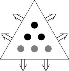
(b) $k=1$

Fig. 1: Element diagrams for $\tilde{\Sigma}_{k+1,h}^{(1)}$ in 2D
gray circle: conforming div-bubble; black circle: nonconforming div-bubble

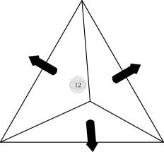
(a) $k=0$

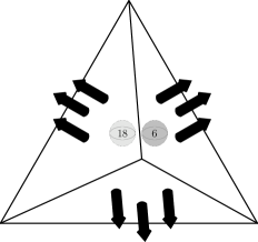
(b) $k=1$

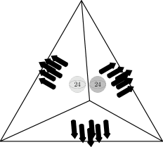
(c) $k=2$

Fig. 2: Element diagrams for $\tilde{\Sigma}_{k+1,h}^{(1)}$ in 3D
dark gray ball: conforming div-bubble; light gray ball: nonconforming div-bubble

For consistency, an interior penalty term is added to the bilinear form, which will improve the convergence order but not affect the stability. One main advantage of these finite elements is their convenience for implementation, since the basis functions of nonconforming face-bubble function spaces can be written explicitly in terms of the orthonormal polynomials. For the case that $k\leq n-1$, we prove that the nonconforming elements have to be applied in the framework that the degree of polynomials for stress are at most $k+1$.

Acknowledgement

The author would like to thank Professor Jun Hu for the helpful discussions and suggestions.

References

- [1] Scot Adams and Bernardo Cockburn, A mixed finite element method for elasticity in three dimensions, Journal of Scientific Computing, 25 (2005), pp. 515–521.
- [2] Mohamed Amara and Jean-Marie Thomas, Equilibrium finite elements for the linear elastic problem, Numerische Mathematik, 33 (1979), pp. 367–383.
- [3] Douglas Arnold and Gerard Awanou, Rectangular mixed finite elements for elasticity, Mathematical Models and Methods in Applied Sciences, 15 (2005), pp. 1417–1429.
- [4] Douglas Arnold, Gerard Awanou, and Ragnar Winther, Finite elements for symmetric tensors in three dimensions, Mathematics of Computation, 77 (2008), pp. 1229–1251.
- [5] , Nonconforming tetrahedral mixed finite elements for elasticity, Mathematical Models and Methods in Applied Sciences, 24 (2014), pp. 783–796.
- [6] Douglas Arnold, Jim Douglas Jr, and Chaitan Gupta, A family of higher order mixed finite element methods for plane elasticity, Numerische Mathematik, 45 (1984), pp. 1–22.
- [7] Douglas Arnold, Richard Falk, and Ragnar Winther, Mixed finite element methods for linear elasticity with weakly imposed symmetry, Mathematics of Computation, 76 (2007), pp. 1699–1723.
- [8] Douglas Arnold and Ragnar Winther, Mixed finite elements for elasticity, Numerische Mathematik, 92 (2002), pp. 401–419.
- [9] , Nonconforming mixed elements for elasticity, Mathematical Models and Methods in Applied Sciences, 13 (2003), pp. 295–307.
- [10] Gerard Awanou, A rotated nonconforming rectangular mixed element for elasticity, Calcolo, 46 (2009), pp. 49–60.
- [11] Ivo Babuška, Error-bounds for finite element method, Numerische Mathematik, 16 (1971), pp. 322–333.
- [12] Daniele Boffi, Franco Brezzi, and Michel Fortin, Reduced symmetry elements in linear elasticity, Commun. Pure Appl. Anal, 8 (2009), pp. 95–121.
- [13] Franco Brezzi, On the existence, uniqueness and approximation of saddle-point problems arising from lagrangian multipliers, Revue française d’automatique, informatique, recherche opérationnelle. Analyse numérique, 8 (1974), pp. 129–151.
- [14] Franco Brezzi and Michel Fortin, Mixed and hybrid finite element methods, no. 15 in springer series in computational mathematics, 1991.
- [15] Zhiqiang Cai and Xiu Ye, A mixed nonconforming finite element for linear elasticity, Numerical Methods for Partial Differential Equations, 21 (2005), pp. 1043–1051.
- [16] Long Chen, iFEM: An Integrated Finite Element Methods Package in MATLAB, technical report, University of California Irvine, 2008.
- [17] Shao-Chun Chen and Ya-Na Wang, Conforming rectangular mixed finite elements for elasticity, Journal of Scientific Computing, 47 (2011), pp. 93–108.
- [18] Bernardo Cockburn, Jayadeep Gopalakrishnan, and Johnny Guzmán, A new elasticity element made for enforcing weak stress symmetry, Mathematics of Computation, 79 (2010), pp. 1331–1349.
- [19] Mohamed Farhloul and Michel Fortin, Dual hybrid methods for the elasticity and the stokes problems: a unified approach, Numerische Mathematik, 76 (1997), pp. 419–440.
- [20] Michel Fortin and Roland Glowinski, Augmented Lagrangian methods: applications to the numerical solution of boundary-value problems, Elsevier, 2000.
- [21] Jayadeep Gopalakrishnan and Johnny Guzmán, Symmetric nonconforming mixed finite elements for linear elasticity, SIAM Journal on Numerical Analysis, 49 (2011), pp. 1504–1520.
- [22] , A second elasticity element using the matrix bubble, IMA Journal of Numerical Analysis, 32 (2012), pp. 352–372.
- [23] Jun Hu, Finite element approximations of symmetric tensors on simplicial grids in : the higher order case, Journal of Computational Mathematics, 33 (2015), pp. 1–14.
- [24] , A new family of efficient conforming mixed finite elements on both rectangular and cuboid meshes for linear elasticity in the symmetric formulation, SIAM Journal on Numerical Analysis, 53 (2015), pp. 1438–1463.
- [25] Jun Hu, Hongying Man, and Shangyou Zhang, A simple conforming mixed finite element for linear elasticity on rectangular grids in any space dimension, Journal of Scientific Computing, 58 (2014), pp. 367–379.
- [26] Jun Hu and Zhong-Ci Shi, Lower order rectangular nonconforming mixed finite elements for plane elasticity, SIAM Journal on Numerical Analysis, 46 (2007), pp. 88–102.
- [27] Jun Hu and Shangyou Zhang, A family of conforming mixed finite elements for linear elasticity on triangular grids, arXiv preprint arXiv:1406.7457, (2014).
- [28] Jun Hu and ShangYou Zhang, A family of symmetric mixed finite elements for linear elasticity on tetrahedral grids, Science China Mathematics, 58 (2015), pp. 297–307.
- [29] Jun Hu and Shangyou Zhang, Finite element approximations of symmetric tensors on simplicial grids in : The lower order case, Mathematical Models and Methods in Applied Sciences, 26 (2016), pp. 1649–1669.
- [30] Claes Johnson and Bertrand Mercier, Some equilibrium finite element methods for two-dimensional elasticity problems, Numerische Mathematik, 30 (1978), pp. 103–116.
- [31] Young-Ju Lee, Jinbiao Wu, Jinchao Xu, and Ludmil Zikatanov, On the convergence of iterative methods for semidefinite linear systems, SIAM journal on matrix analysis and applications, 28 (2006), pp. 634–641.
- [32] Hong-Ying Man, Jun Hu, and Zhong-Ci Shi, Lower order rectangular nonconforming mixed finite element for the three-dimensional elasticity problem, Mathematical Models and Methods in Applied Sciences, 19 (2009), pp. 51–65.
- [33] Weifeng Qiu and Leszek Demkowicz, Mixed hp-finite element method for linear elasticity with weakly imposed symmetry, Computer Methods in Applied Mechanics and Engineering, 198 (2009), pp. 3682–3701.
- [34] L Ridgway Scott and Shangyou Zhang, Finite element interpolation of nonsmooth functions satisfying boundary conditions, Mathematics of Computation, 54 (1990), pp. 483–493.
- [35] Son-Young Yi, Nonconforming mixed finite element methods for linear elasticity using rectangular elements in two and three dimensions, Calcolo, 42 (2005), pp. 115–133.
- [36] , A new nonconforming mixed finite element method for linear elasticity, Mathematical Models and Methods in Applied Sciences, 16 (2006), pp. 979–999.