Ab initio calculation of the shock Hugoniot of bulk silicon

Abstract

We describe a simple annealing procedure to obtain the Hugoniot locus (states accessible by a shock wave) for a given material in a computationally efficient manner. We apply this method to determine the Hugoniot locus in bulk silicon from ab initio molecular dynamics with forces from density-functional theory, up to $70\text{\;}\mathrm{G}\mathrm{P}\mathrm{a}$. The fact that shock waves can split into multiple waves due to phase transitions or yielding is taken into account here by specifying the strength of any preceding waves explicitly based on their yield strain. Points corresponding to uniaxial elastic compression along three crystal axes and a number of post-shock phases are given, including a plastically-yielded state, approximated by an isotropic stress configuration following an elastic wave of predetermined strength. The results compare well to existing experimental data for shocked silicon.

I Introduction

Shock waves are used extensively to study matter at conditions of extreme pressure and temperature, and have been used to obtain some of the highest laboratory-attained pressures. They are useful for equation of state determination and are important dynamic phenomena in their own right, arising in aerodynamics,Dolling (2001) reactive flowDlott (2011) and high-speed impact.Duvall and Graham (1977); Asay and Shahinpoor (1993)

Simulations of shock waves have a long history.Holian (2004) Direct simulations using empirical potentials are now feasible on a multi-billion atom scale on present hardware, which is large enough to observe detailed mechanisms of yield, plastic flow and shock interaction with nanostructures, directly.Kadau et al. (2006); Shekhar et al. (2013) Work with empirical potentials can give important insight and understanding, but a need for first-principles methods such as Density Functional Theory (dft) exists in providing predictive power and accuracy. These methods must use more modest system sizes, of hundreds or thousands of atoms in the case of dft.

Silicon has a rich phase diagram, with metallic dense phases rather different in character to the ambient diamond phase, making it an interesting and challenging object of simulation. In total, eleven stable or metastable phases of silicon are currently known.Mujica et al. (2003) Shock experiments have provided important data for constructing the phase diagram. The phase transition in silicon from the cubic diamond structure to the beta-tin structure, occurring at $12\text{\;}\mathrm{G}\mathrm{P}\mathrm{a}$ at room temperature, and undergoing a reduction in volume of 20%, has been well established by static loading experiments from the 1960s onward.Minomura and Drickamer (1962); Jamieson (1963) Evidence of at least one phase transition at similar pressures was then observed in shock-wave experiments, starting with Pavlovskii (. 1968)

If a shock wave is strong enough to cause a material to yield plastically or undergo a phase transition, the wave can split into two or more separate shock waves, and this has long been observed and understood.Duvall and Graham (1977) In this situation, the last shock takes the material to its final state, but the preceding shocks take the material to a cusp on the pressure-volume Hugoniot locus caused by a transition: either the Hugoniot elastic limit or the onset pressure of a phase transition. In silicon, Gust and Royce (1970, 1971) found a three-wave structure for samples shocked in the $\langle\text{100}\rangle$ crystal direction and a four-wave structure when shocked in the $\langle\text{110}\rangle$ or $\langle\text{111}\rangle$ directions. In the latter cases, these waves were attributed to: an initial elastic precursor to the Hugoniot elastic limit of $5.5\text{\;}\mathrm{G}\mathrm{P}\mathrm{a}$, followed by waves corresponding to a state of plastic yield and two successive phase transitions at $10\text{\;}\mathrm{G}\mathrm{P}\mathrm{a}$ and $13\text{\;}\mathrm{G}\mathrm{P}\mathrm{a}$. Along $\langle\text{100}\rangle$, the higher elastic limit of $9\text{\;}\mathrm{G}\mathrm{P}\mathrm{a}$ obscures the first transition wave, and a single wave takes the material simultaneously to a new phase and to a state of hydrostatic stress.

The work of Goto et al. (1982) largely confirmed the findings of Gust and Royce (, 1971) although they observed a three-wave structure, regardless of crystal orientation, consistent with only a single phase transition at $13\text{\;}\mathrm{G}\mathrm{P}\mathrm{a}$. Above the Hugoniot elastic limit, shock compression was found to result in a hydrostatic stress configuration, due to the complete loss of strength in the material.

More recently, and contrary to the earlier experimental work, Turneaure and Gupta (2007a, b) reported a single phase transition that is complete by $15.9\text{\;}\mathrm{G}\mathrm{P}\mathrm{a}$. Shocks to these pressures show a much greater volume compression than the points attributed to an extended mixed-phase region by both Gust and Royce (1971) and Goto et al. (1982) Here the phase transition is not complete until at least $30\text{\;}\mathrm{G}\mathrm{P}\mathrm{a}$. This discrepancy is explained by Turneaure and Gupta (2007b) as arising from the reflection of the first two shock waves propagating back into the material before the arrival of the third wave, and altering the peak state of the earlier experiments. They avoid this eventuality by backing the silicon with a window made from lithium fluoride, a material with a good impedance match to silicon.

The Imma phase of silicon is found intermediate between the beta-tin and simple hexagonal phases, and is stable between $13\text{\;}\mathrm{G}\mathrm{P}\mathrm{a}$ and $15\text{\;}\mathrm{G}\mathrm{P}\mathrm{a}$ at room temperature.McMahon et al. (1994) Theoretically, the energy and volume of these three phases are close.Mujica et al. (2003) A recent simulation of directly shocked silicon using an empirical potentialMogni et al. (2014) found a phase transition to an Imma phase with a modification of the Tersoff potentialTersoff (1986, 1988) of Erhart and Albe (. 2005)

In this paper, we give the Hugoniot loci according to Density Functional Theory for several pure phases of silicon, including cubic diamond under elastic compression along $\langle\text{100}\rangle$, $\langle\text{110}\rangle$ and $\langle\text{111}\rangle$, a hydrostat (resulting from either a single shock or a split-shock structure), beta-tin, simple hexagonal and the liquid, and report shock temperatures for these states.

Several approaches can been taken for the determination of a Hugoniot locus from molecular dynamics. The most straightforward, but computationally the most demanding, is to simulate a slab of atoms struck by an impactor directly, measuring the speed of any shock waves and post-shock average particle velocities as they arise from the simulation. From the Hugoniot relations, these velocities can be converted to a relationship between pressure and volume compression. For empirical potentials, a local stress is conveniently available, so this could also be taken directly from the simulation. This is the approach taken by, e.g. Kadau et al. (2007)

It is simple to check that a given equilibrium state lies on or close to the (single-shock) Hugoniot locus, which amounts to satisfying the Hugoniot relation

$$E-E_{0}=-\frac{1}{2}(\sigma^{33}+\sigma^{33}_{0})(V_{0}-V),$$ (1)

where $E$ is the internal energy, $V$ is the specific volume and $\sigma^{33}$ is the stress in the direction of the shock (and can be replaced with the pressure $p$ in a hydrostatic situation). The zero-subscripted variables are for the pre-shocked state. Other (equivalent) Hugoniot relations exist between any three of: internal energy, pressure, volume, shock velocity and particle velocity. It is therefore sufficient to sample several points that are chosen to bracket the Hugoniot locus, and the Hugoniot state then approximated by interpolation, or solved for iteratively. The former is the approach taken by Bonev et al. (2004) for shocked deuterium.

Swift et al. (2001) constructed a polymorphic equation of state for silicon, incorporating dft simulations of the cubic diamond and $\beta$-Sn phases, with the lattice-thermal contribution approximated by quasiharmonic phonons. The equation of state was constructed with a particular focus on simulating shock waves. The full equation of state was sampled and the Hugoniot locus could therefore be extracted as a one-dimensional path through it. The phase boundary and mixed phase region along the Hugoniot were found explicitly by minimizing the Helmholtz free energy computed from the quasiharmonic phonon approximation.

Alternatively, a Hugoniot state can be determined dynamically from within a single molecular dynamics simulation by some modified dynamics to constrain the state to satisfy eq. 1. This is the approach taken by the Hugoniostat methodsMaillet et al. (2000); Ravelo et al. (2004) and the technique of Reed et al. (2003) The former simulations use modified Nosé–Hoover dynamics while the latter uses coupled dynamics of the atoms and simulation cell, whose Lagrangian involves the computed instantaneous shock speed, and varies the simulation cell uniaxially. One aim of these dynamics is to work on timescales comparable to shock-passage times, without the overhead of dealing with a direct non-equilibrium simulation.

If we are interested only in the final post-shock state, and are not interested in the (modified) dynamics while the constraint is being applied, we are free to use a method based on simple velocity rescaling, analogous to the procedure of Berendsen,Berendsen et al. (1984) which is what we propose here due to its increased efficiency in reaching the final state.

II Computational Method

II.1 Density Functional Theory

The ab initio md simulations described here were performed with the Siesta method and implementation of Density Functional Theory, Soler et al. (2002) using the Perdew et al. (1996) gga functional.

Table 1: Basis parameters for silicon, according to the soft-confinement scheme of Junquera et al. (2001). For the purposes of basis generation, an effective ionic charge of -0.46 was used, which was also variationally optimized. The cutoff radii of the first and second zeta functions are $r(\zeta_{1})$ and $r(\zeta_{2})$, and $r_{i}$ is the confinement potential’s internal radius. $V_{0}$ is the soft-confinement prefactor.

$n$	$l$	$r_{i}$ ($a_{0}$)	$r(\zeta_{1})$ ($a_{0}$)	$r(\zeta_{2})$ ($a_{0}$)	$V_{0}$ (Ry)
3	0	4.97	7.00	4.38	15.43
3	1	3.83	7.00	4.09	04.70
3	2	0.03	4.55	-	11.97

The core electrons were described with a Troullier–Martins norm-conserving pseudopotentialTroullier and Martins (1991) with a matching radius in each angular momentum channel of $1.89\text{\;}\mathrm{a}_{\mathrm{0}}$. The valence electrons were described with a basis of numerical atomic orbitals of double-$\zeta$ polarized typeJunquera et al. (2001) (representing 13 orbitals per atom). The basis was generated by fixing the longest orbital cutoffs at $7.0\text{\;}\mathrm{a}_{\mathrm{0}}$ and variationally optimising the other parameters in bulk diamond-phase silicon—the final basis parameters are given in table 1.

The mesh used for integrals in real-space was well converged at a grid cutoff of $100\text{\;}\mathrm{R}\mathrm{y}$. The dense phases of silicon required several $k$-points to converge in energy, and in particular, for the cold compression curves of the various phases to converge in energy relative to one another. A $4^{3}$ Monkhorst–Pack grid of points was used on the 64 atom simulations, to give an effective cutoff length of $21\text{\;}\mathrm{\SIUnitSymbolAngstrom}$.

The electronic temperature used in the dft calculations should be consistent with the final temperature attained after the annealing process described below. The consistent forces for the ab initio molecular dynamics are the nuclear-position derivatives of the electronic free-energy as defined in Mermin’s dft.Mermin (1965) All of the simulations reported below are for an electronic temperature of $300\text{\;}\mathrm{K}$, except for the two points with highest temperatures, for which the electronic temperature was adjusted to coincide with the final (nuclear) temperature. The effect of the electronic temperature on the reported quantities was found to be quite small: the maximum difference in pressure for the hottest simulation between using a consistent electronic temperature and the initial $300\text{\;}\mathrm{K}$ is below 5%.

The integration of the dynamics used the Born-Oppenheimer approximation with a timestep of $1\text{\;}\mathrm{f}\mathrm{s}$.

II.2 Annealing to the Hugoniot Locus

We use a simple annealing procedure to find the state on the Hugoniot corresponding to a specified longitudinal strain. A Berendsen thermostatBerendsen et al. (1984) is used with a variable target temperature computed from the instantaneous difference in energy between the total energy of the system, and the total energy that would be required to satisfy the energy Hugoniot relation, eq. 1, exactly, given the current instantaneous longitudinal stress.

The procedure is given explicitly below. This may be combined with a further anneal to relax the pressure to a hydrostatic configuration if desired. Optionally, the box vectors may be gradually ramped between two states, which is most useful when the starting state of the simulation and the initial state of the Hugoniot locus are the same.

procedure HugoniotAnneal($E^{\text{tot}}_{0},V_{0},\sigma_{0}$)

     compute $E^{\text{tot}},\varsigma,\bm{F}_{n}$ from atomic positions $\bm{x}_{n}$

     for all atoms do $\triangleright$ velocity Verlet

         $\bm{v}_{n}\leftarrow\bm{v}_{n-1}+\dfrac{\mathrm{d}{}t}{2m}(\bm{F}_{n-1}+\bm{F}_{n})$

         $\bm{x}_{n+1}^{\text{(unc)}}\leftarrow\bm{x}_{n}+\mathrm{d}{}t\,\bm{v}_{n}+\dfrac{\mathrm{d}{}t^{2}}{2}\bm{F}_{n}/m$

     end for

     $\sigma\leftarrow\frac{1}{V}\sum_{\text{atoms}}m\,\bm{v}_{n}\otimes\bm{v}_{n}+\varsigma$ $\triangleright$ compute the stress

     $E^{\text{kin}}\leftarrow\sum_{\text{atoms}}\frac{1}{2}m\,\bm{v}_{n}\cdot\bm{v}_{n}$

$\triangleright$ compute the target energy

     $E^{\text{hug}}\leftarrow E^{\text{tot}}_{0}-\frac{1}{2}(\sigma^{33}+\sigma^{33}_{0})(V_{0}-V)$

     $E^{\text{kin}}_{\text{target}}\leftarrow E^{\text{kin}}+E^{\text{hug}}-E^{\text{tot}}$

     $r^{2}\leftarrow\left(1+\dfrac{\mathrm{d}{}t}{\tau_{\text{relax}}}\left(\dfrac{E^{\text{kin}}_{\text{target}}}{E^{\text{kin}}}-1\right)\right)$

     for all atoms do

         $\bm{v}_{n}^{\text{(sca)}}\leftarrow r\bm{v}_{n}$ $\triangleright$ scale the velocities

$\triangleright$ correct positions based on the scaled velocities

         $\bm{x}_{n+1}\leftarrow\bm{x}_{n+1}^{\text{(unc)}}+\mathrm{d}{}t\,(\bm{v}_{n}^{\text{(sca)}}-\bm{v}_{n})$

     end for

     $t\leftarrow t+\mathrm{d}{}t$, $n\leftarrow n+1$

end procedure

The meaning of the variables used is as follows. $E$ denotes an energy (refer to the sub and superscripts), $V$ is the unit cell volume, $\sigma$ is the stress, which is the sum of a kinetic term and the strain derivative of the total electronic energy $\varsigma$; $\bm{x}_{n}$, $\bm{v}_{n}$ and $\bm{F}_{n}$ are the atomic positions, velocities and forces at the $n$th timestep (‘unc’ stands for ‘uncorrected’ and ‘sca’ for scaled), $m$ is the mass of a given atom, $\tau_{\text{relax}}$ is the relaxation time, $t$ and $\mathrm{d}{}t$ are the current time and timestep, and anything with a subscript ‘$0$’ refers to its (time averaged) value in the unshocked state (which may be different from the starting state of the simulation).

Even though Berendsen thermo- and barostats do not reproduce canonical statistics,Harvey et al. (1998) it is well known that they are much more efficient at annealing to a given equilibrium state at a desired temperature or pressure compared with modified dynamics, such as Nosé–Hoover. The same applies here, compared to the related Hugoniostat for shocks, and this justifies their use, since we are interested only in the outcome of the anneal, not the intermediate dynamics. After the time-averaged state of the system closely satisfies the Hugoniot relation, the simulation can be restarted with Verlet dynamics to check if eq. 1 is indeed satisfied.

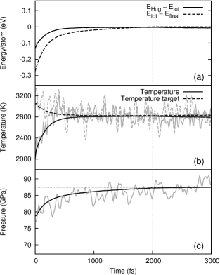
Figure 1: Response of (a) internal energy and the difference with the Hugoniot energy computed from eq. 1, (b) temperature and target temperature, and (c) pressure, to the Hugoniot anneal described here with a relaxation time of $100\text{\;}\mathrm{f}\mathrm{s}$. After $2000\text{\;}\mathrm{f}\mathrm{s}$, the anneal is switched off and the dynamics continued with Verlet integration. The response is averaged over $10\,000$ independent 216 atom Stillinger–Weber silicon systems, starting from a $2000\text{\;}\mathrm{K}$ liquid and annealed to the Hugoniot locus with an initial state of $300\text{\;}\mathrm{K}$ and zero stress. For comparison, the light grey lines are taken from a single trajectory—in the energy plot, this is indistinguishable from the mean.

Figure 1 shows the convergence in total energy, temperature and pressure of liquid Stillinger-Weber silicon to a state on the particular Hugoniot locus from an initial state of $300\text{\;}\mathrm{K}$ and zero pressure. This is an averaged result of $10\,000$ independent simulations, each starting in the liquid phase at $2000\text{\;}\mathrm{K}$. The relaxation time used was $100\text{\;}\mathrm{f}\mathrm{s}$. After $2000$ timesteps of $1\text{\;}\mathrm{f}\mathrm{s}$, the anneal is switched off and Verlet integration used for the remaining time. Note the slight relaxation of temperature and pressure away from their final values under the thermostat. For this case, it amounts to a temperature difference of within 1%.

III Results

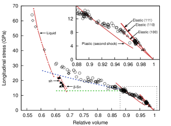
Figure 2: Pressure–volume Hugoniot loci for silicon. The solid red lines in the figure are the dft results from this work (with contained points indicating individual simulations), with an initial pre-shocked state of zero pressure and $300\text{\;}\mathrm{K}$, with the final state in the indicated phase (‘sh’ for simple hexagonal). Estimated error is less than 5% for the liquid and beta-tin phases, and is substantially smaller for the diamond phase. The symbols are experimental results from the literature: $\circ$ Gust and Royce (1971), $\diamond$ Goto et al. (1982), $\triangle$ Turneaure and Gupta (2007a), $\blacktriangle$ Turneaure and Gupta (2007b). The dashed lines are approximations to the mixed-phase portion of the Hugoniot, for cubic diamond to: liquid (upper blue line) and beta tin (lower green line).

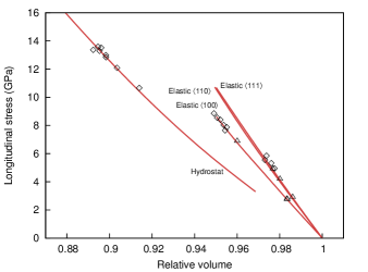
Figure 3: Pressure–volume Hugoniot loci for silicon. This is a similar plot to fig. 2, with the meaning of the symbols and lines the same, emphasizing the small strain region of the Hugoniot locus and with the results of Gust and Royce (1971) omitted due to their larger variance.

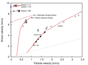
Figure 4: Particle velocity–shock velocity Hugoniot loci for silicon. The dft results (solid red lines and points) each correspond to an initial state of zero pressure and $300\text{\;}\mathrm{K}$, with the final state in the indicated phase. The dashed line is for a single-shock process whose final state has a hydrostatic stress configuration. The meaning of the symbols is the same as in fig. 2, with the blue diamonds on the axis the elastic and bulk wave speeds from Goto et al. (1982) The dotted base line indicates equal shock and particle velocity, below which no viable shock should be recorded.

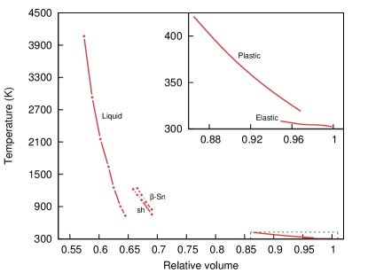
Figure 5: Post-shock temperature as a function of volume for several final states. The dft results (solid red lines) each correspond to an initial state of zero pressure and $300\text{\;}\mathrm{K}$, with the final state in the indicated phase. The ‘plastic’ curve does not include the temperature rise due to dissipative heating. The meaning of the symbols is the same as in fig. 2

The calculated pressure–volume and shock-velocity–particle-velocity Hugoniot loci for the pure phases are compared to results from several experiments in figs. 2, 3 and 4. The specific volume at zero pressure and $300\text{\;}\mathrm{K}$ for the pbe functional is $0.421\text{\;}\mathrm{c}\mathrm{m}^{3}\mathrm{/}\mathrm{g}$, which is smaller than the experimental value of $0.431\text{\;}\mathrm{c}\mathrm{m}^{3}\mathrm{/}\mathrm{g}$. The reduced volume is plotted in the figures: if the specific volume were plotted instead, the dft results would be offset by an amount corresponding to the difference in zero-pressure volume. The particle velocity–shock velocity Hugoniot is not greatly affected.

The curves for the elastic shocks are computed from a uniaxial box deformation along the indicated direction. The ‘plastic’ curve is for a split shock, with an elastic precursor to $6\text{\;}\mathrm{G}\mathrm{P}\mathrm{a}$, taking the material to a hydrostatic stress configuration: this supposes that the material has no residual strength. The hydrostat in fig. 4 is for an unphysical shock process that relaxes the material to hydrostatic stress behind a single, unsplit shock wave. This permits comparison with the bulk speed of sound (the shock velocity for this wave should extrapolate to the bulk speed of sound at zero particle velocity.)

When comparing the hydrostat and the ‘plastic’ curve to the yielded phase, we assume that the yielding serves only to remove the deviatoric stress, and that the bulk response of the material is unaffected. We neglect the dissipative heating due to this effect.

The agreement with the experimental data for the elastic and plastic shocks is good, with the compressibility along $\langle\text{100}\rangle$, $\langle\text{110}\rangle$ matching well in value and $\langle\text{111}\rangle$ showing the correct trend (although underestimating the value). The close match between the experimental plastic shock pressures and the hydrostatic plastic shock calculated here supports the observation that the material loses all of its strength after yield.

Table 2: Coefficients of a linear fit the shock velocity for the elastic waves, $U_{s}=c_{0}+su_{p}$, for this work and two sets of experimentally-determined values.

	$\langle\text{100}\rangle$		$\langle\text{110}\rangle$		$\langle\text{111}\rangle$		Bulk
	$c_{0}$	$s$	$c_{0}$	$s$	$c_{0}$	$s$	$c_{0}$	$s$
	($\mathrm{k}\mathrm{m}\mathrm{/}\mathrm{s}$)	(-)
This work	8.38	0.42	9.21	0.57	9.34	0.57	6.51	1.18
Ref. Goto et al.,1982	8.42	0.32	9.24	1.01	9.39	0.98	-
Ref. Hall,1967	8.43	-	9.13	-	9.34	-	6.48	-

The particle and shock velocities in fig. 4 are computed from the computed pressure and volume points using the Hugoniot relations

$$u_{p}^{2} =(p-p_{0})(v_{0}-v)$$ (2)

$$U_{s}^{2} =v_{0}^{2}(p-p_{0})/(v_{0}-v),$$ (3)

where $v_{0}$ and $v$ are the initial and final specific volumes. A linear fit to the elastic part of the shock-velocity–particle-velocity Hugoniot has coefficients given in table 2. The extrapolated value of the bulk sound speed of $6.51\text{\;}\mathrm{km}\text{\,}{\mathrm{s}}^{-1}$ agrees very well with the value of $6.48\text{\;}\mathrm{km}\text{\,}{\mathrm{s}}^{-1}$ calculated from the second order elastic constants.Gust and Royce (1971); Hall (1967)

The $\beta$-Sn and simple hexagonal curves each correspond to a three wave split shock structure, behind an elastic wave to the experimental elastic limit of $6\text{\;}\mathrm{G}\mathrm{P}\mathrm{a}$ and a secondary wave to the experimental location of the phase transition at $13.8\text{\;}\mathrm{G}\mathrm{P}\mathrm{a}$. For both of these waves, the computed volume for the $\langle\text{100}\rangle$ direction was used for the post-shock state. In general, it is quite insensitive to the precise location of the wave split, particularly for the elastic case, since the contribution to the energy change is much smaller than the 20% volume reduction across the phase change. The final stress was hydrostatic. Since the $c/a$-ratio is free in the $\beta$-Sn and simple hexagonal structures, an additional relaxation step was used on the simulation box to impose a hydrostatic distribution of stress while simultaneously annealing to the Hugoniot. The $\beta$-Sn and simple hexagonal curves are close in pressure, temperature and shock velocity, with the experimental values closest to the simple hexagonal dft Hugoniot. The computed pressures and temperatures of these points put them in stable region for the simple hexagonal structure on the silicon phase diagram.Kubo et al. (2008)

Part of the liquid Hugoniot corresponds to a three-wave shock structure, with the third wave reaching the final liquid state, behind a secondary wave to the onset of the melting transition and an elastic precursor wave. For the highest pressures, where the final wave has a velocity greater than that of the secondary wave of $6.83\text{\;}\mathrm{k}\mathrm{m}\mathrm{/}\mathrm{s}$, it instead corresponds to a two-wave structure (behind only the elastic precursor). The largest shock pressures closely match the calculated liquid Hugoniot, with the simulated liquid being systematically slightly too stiff.

The predicted post-shock temperatures (given in fig. 5) indicate that these highest pressure points are likely to be liquid phase. The sixfold coordinated liquid lies close in $p$–$v$ to the Hugoniot for the beta-tin phase, and so this phase transition does not exhibit the large mixed phase region as for the diamond to dense-phase silicon.

III.1 The Phase Transition

There is a considerable range of relative volume between the Hugoniot loci of the pure phases shown in fig. 2. The experimentally measured points in this region have a final state that is a mixture of two phases. Points on the mixed-phase region of the Hugoniot are on the intersection of the phase boundary for the two phases, as well as satisfying eq. 1.

Similar to the plastic shock, a pressure–volume Hugoniot is convex at the onset of a mixed phase region: if the change in slope is great enough, this causes the shock to split into a wave taking the material to the pressure at the onset of the phase transition, and a slower wave taking the material to its final state, which is a coexistence of the two phases.

The Hugoniot locus through the mixed phase region can be constructed by considering the jump condition in enthalpy across the shock from the point (‘1’) at the onset of the transition to a point (‘2’) on the mixed Hugoniot

$$H_{2}-H_{1}=E_{2}-E_{1}+p_{2}V_{2}-p_{1}V_{1},$$ (4)

and on substituting eq. 1 for the jump in internal energy, this reduces to

$$H_{2}-H_{1}=\frac{1}{2}(p_{2}-p_{1})(V_{2}+V_{1}).$$ (5)

The latent heat $L$ of the phase transition results in a change in enthalpy, written according to the Clausius–Clapeyron equation as

$$\lambda L=-T\frac{\mathrm{d}p}{\mathrm{d}T}(V_{1}-V_{2}),$$ (6)

where $\lambda$ is the mass fraction of the second phase and the derivative is along the phase line.

Since the mixed region is not at constant pressure, there is an additional contribution to the enthalpy change from the difference in pressure and volume between the onset of the transition and the post-shock state. This leads to a linearized equation relating the pressure and volume changes on the phase-transition shock,Duff and Minshall (1957)

$$p_{2}-p_{1}=(V_{1}-V_{2})\times\\ \left[\beta V_{1}+\left(\frac{1}{2T_{1}}(V_{1}-V_{2})-2\alpha V_{1}\right)\frac{\mathrm{d}T}{\mathrm{d}p}+\frac{C_{p}}{T_{1}}\left(\frac{\mathrm{d}T}{\mathrm{d}p}\right)^{2}\right]^{-1},$$ (7)

where $\beta$ is the isothermal compressibility, $\alpha$ is the volumetric thermal expansion coefficient and $C_{p}$ is the heat capacity at constant pressure. The derivative $\mathrm{d}{T}/\mathrm{d}{p}$ is once again along the phase boundary.

We require knowledge of the onset of the transition in the $p$–$V$ plane, which is not available from the single phase simulations alone (the simulated materials are capable of being substantially superheated or supercooled). This could be obtained from the point where the Hugoniot cuts the phase boundary obtained by some other method.

Table 3: Summary of values used at the onset of the cubic diamond to liquid phase transition. The phase line is as obtained by the experiment of Kubo et al. (2008). The other values are from Hull (1999), with $\alpha$ and $c_{p}$ at $1600\text{\;}\mathrm{K}$ and ambient pressure, and $\beta$ at $298\text{\;}\mathrm{K}$ and $13.8\text{\;}\mathrm{G}\mathrm{P}\mathrm{a}$.

$T$ ($\mathrm{K}$)	$dT/dP$ ($\mathrm{K}\mathrm{G}\mathrm{P}\mathrm{a}^{-1}$)	$\alpha$ ($\mathrm{K}^{-1}$)	$\beta$ ($\mathrm{G}\mathrm{P}\mathrm{a}^{-1}$)	$c_{p}$ ($\mathrm{J}\mathrm{g}^{-1}\mathrm{K}^{-1}$)
1683	62.4	$4.5\text{\times}{10}^{-6}$	0.024	1.0

We consider here two possible phase transitions starting from silicon in the cubic diamond structure: to a liquid, and to the beta-tin structure. In addition, we assume that the onset of either transition occurs at $13.8\text{\;}\mathrm{G}\mathrm{P}\mathrm{a}$, close to the observed experimental value. The phase lines are experimental values, obtained by Kubo et al. (2008) This gives the two dashed lines appearing in fig. 2. The lower, green dashed line for diamond structure to beta-tin is nearly at constant pressure, since its slope is dominated by the steep phase-line of the transition,Kubo et al. (2008) $dT/dp=$-1426\text{\;}\mathrm{K}\mathrm{/}\mathrm{G}\mathrm{P}\mathrm{a}$$. This is consistent with the experiment of Turneaure and Gupta (. 2007b) The upper, blue dashed line for melting the diamond structure is influenced most strongly by the compressibility $\beta$ of the cubic diamond phase at the pressure and temperature of the onset. Representative literature values for the constants appearing in the above expression for the liquid are summarized in table 3. This line underestimates the experimentally observed slope seen by Gust and Royce (1971) and Goto et al. (1982) While the simulated temperature at this pressure is much too low for melting, the simulations of the ‘plastically-yielded’ state do not include dissipative heating and this could cause a considerable temperature rise above those reported in fig. 5.

IV Conclusion

In conclusion, we have described a simple annealing method and shown that it may be used to obtain a state on the Hugoniot locus of a pure phase of a material with several condensed phases efficiently, from first-principles. An approximation relying on the slope of the phase boundary can be used to obtain the part of the Hugoniot corresponding to coexistence between two phases.

In the case of silicon, the results computed using this procedure with the forces described using density functional theory match existing experimental data very well for pressures up to $60\text{\;}\mathrm{G}\mathrm{P}\mathrm{a}$, the limit of available experimental data. We have provided a prediction of the shock temperatures of silicon over this pressure range. This study supports the conclusions of the experimental work in general, that silicon after yield supports no deviatoric stress, and of Turneaure and Gupta (, 2007b) that the first observed phase transition along the shock locus is likely to be to simple hexagonal.