Stellar Spiral Structures in Triaxial Dark Matter Haloes

Abstract

We employ very high resolution simulations of isolated Milky Way-like galaxies to study the effect of triaxial dark matter haloes on exponential stellar discs. Non-adiabatic halo shape changes can trigger two-armed grand-design spiral structures which extend all the way to the edge of the disc. Their pattern speed coincides with the inner Lindblad resonance indicating that they are kinematic density waves which can persist up to several Gyr. In dynamically cold discs, grand-design spirals are swing amplified and after a few Gyr can lead to the formation of (multi-armed) transient recurrent spirals. Stellar discs misaligned to the principal planes of the host triaxial halo develop characteristic integral shaped warps, but otherwise exhibit very similar spiral structures as aligned discs. For the grand-design spirals in our simulations, their strength dependence with radius is determined by the torque on the disc, suggesting that by studying grand-design spirals without bars it may be possible to set constraints on the tidal field and host dark matter halo shape.

1 Introduction

For many years spiral structures in galaxies have been the subject of extensive observational, theoretical and numerical studies, but their origin still remains unclear. While the morphologies of spiral structures vary considerably, they can be generally classified into two broad categories: ‘grand-design’ spirals with mostly two arms that extend over a large range of radii and ‘flocculent’ spirals that consist of many small fragments of arms. Both kinds of spirals are mostly trailing rather than leading.

Theories of formation and evolution of spirals fall into two categories: (a) self-induced spiral formation, in which spiral structures form due to gravitational interaction between finite number of stars, and (b) externally driven spiral formation, in which spiral structures form as a response to external perturbations.

Lindblad proposed a theory of quasi-stationary spiral structures for grand-design spirals (e.g. Lindblad, 1963). In his theory, spiral structures are in fact kinematic density waves with a pattern speed of $\Omega_{\mathrm{P}}=\Omega-\kappa/n$, where $\Omega$ is the corotation velocity, $\kappa$ is the epicyclic frequency and $n$ is the number of arms (typically equal to 2). In a frame moving with this pattern speed, the orbits of the epicyclic motion of the stars become ellipses without precession, which guarantees that the density field of the disc remains constant in this rotating frame. When orbits are arranged in a way that the highest density falls into a spiral-like shape (e.g. Kalnajs, 1973), constantly rotating stationary grand-design spiral structures can survive in the disc (Lindblad, 1956). Lin & Shu (1964) developed a theory of density waves of quasi-stationary spiral structures further. They regarded spiral structures as large-scale waves propagating through the disc in a linear regime (see also Bertin & Lin, 1996).

‘Flocculent’ spiral structures (and some of the ‘grand-design’ spirals) are considered to be caused by instabilities due to self-gravity. To form spiral structures of this kind, two important processes are needed: swing amplification of small perturbations and a feedback loop. The local stability of a razor-thin disc with respect to axisymmetric tightly wound perturbations is characterized by Toomre’s $Q$ parameter (Toomre, 1964). For stellar discs, we have

$$Q=\frac{\sigma_{R}\kappa}{3.36\,G\Sigma},$$ (1)

where $\sigma_{R}$ is the velocity dispersion in the radial direction and $\Sigma$ is the surface density. When $Q>1$, the disc is locally stable to axisymmetric perturbations, while for $Q<1$, the disc becomes locally unstable. Considering the case of non-axisymmetric perturbations, Julian & Toomre (1966) studied the stability of differentially rotating discs and showed that due to self-gravity, small perturbations can be greatly amplified. Toomre (1981) explored the theory further and showed that strong swing amplification can occur when $Q$ is slightly higher than 1, i.e. if the disc is locally stable but the self-gravity is still strong and the wavelength ratio $X$ is appropriate (typically between 1 and 3):

$$X=\frac{k_{\mathrm{crit}}R}{m}=\frac{\kappa^{2}R}{2\uppi G\Sigma m}\,,$$ (2)

where $R$ is the radius, $m$ is the number of arms and $k_{\mathrm{crit}}=\kappa^{2}/(2\uppi G\Sigma)$ is the critical wavelength of the swing amplification. In this process small leading waves are amplified to strong trailing waves and the amplification factor can be as high as 100. Toomre (1981) also demonstrated that swing amplification can act on global spiral patterns and greatly amplify their strength, though external torques, for example, are sufficient to form those patterns. Similarly, Grand et al. (2012a) showed that two-armed spiral structures in barred galaxies can be dominated by swing amplification.

Recent studies combining numerical and analytic efforts have further shown that stars interact with each other over long periods of time through resonances. Sellwood (2012) found that stars are scattered at the inner Lindblad resonance as the transient spiral structures form, leading to a re-distribution in the action space. When stars are rotated randomly to erase non-axisymmetric features without affecting the distribution in action space, spiral structures restore rapidly, indicating that the scattering at inner Lindblad resonance is more fundamental than the change in the density field. Such a scattering has been recently studied by Fouvry & Pichon (2015) using a dressed Fokker–Planck formalism, which offers a powerful tool to probe the evolution of discs as a function of their properties.

While a number of past numerical studies found that spirals fade out quickly over time (for a recent review see Dobbs & Baba, 2014, and references therein), recent studies showed that in a stellar disc with more than a few million particles spiral arms persist for longer periods of time, indicating that previous results were suffering from discreteness effects (e.g. Fujii et al., 2011; Grand et al., 2012b). D’Onghia et al. (2013) showed that with a sufficiently high number of particles (of the order of $10^{8}$), stellar discs with $Q$ slightly larger than $1$ can stay stable over a few galactic years. When, however, density perturbations are introduced in the disc (in the form of heavy particles), a transient spiral pattern forms which itself can act as the source of newly formed spiral arms. Sellwood & Carlberg (2014) studied the power spectra of such transient spirals, and found that they are superposition of several rigid rotating modes lying between the inner and the outer Lindblad resonance. They also found that such waves scatter particles towards new regions of a disc, thus changing the impedance of the disc, reflecting the waves and hence giving rise to new standing waves. In fact, Fouvry et al. (2015) showed that such simulations of spiral structures dominated by self-gravity in discrete discs can be characterized by the Balescu–Lenard equation, whose predictions on the properties of the secular orbital diffusion agree very well with simulations.

Taken together, these recent numerical works indicate that to study stellar spiral structures that may form in response to external perturbations, discs need to be represented with a very high number of resolution elements, to both minimize arteficial spiral heating and the Poisson noise in the initial conditions, ensuring that the growing time of transient spirals is long enough compared to the evolution of grand-design spirals.

For the triggering mechanism of the grand-design spiral structures, additionally to bars (e.g. Salo et al., 2010; Athanassoula, 2012) and close companions (e.g. Purcell et al., 2011), torques caused by the host dark matter halo have been invoked as well. Even though the properties of dark matter haloes, such as their exact shape and mass distribution (and the back-reaction of baryons), are still not precisely known, already early work (e.g. Binney, 1978; Barnes & Efstathiou, 1987; Frenk et al., 1988) have indicated that the haloes are generally triaxial. Follow-up studies with a variety of configurations, including dispersionless gravitational collapse models (Warren et al., 1992), self-interacting dark matter models (Yoshida et al., 2000), haloes formed in different cosmological models (Jing et al., 1995; Thomas et al., 1998), and more recent higher-resolution studies (e.g. Bryan et al., 2013; Zhu et al., 2016) all find that the dark matter haloes are triaxial. Several generalizations of analytical, spherical halo models that include halo triaxiality were also proposed Jing & Suto, 2002; Bowden et al., 2013. Analysing high resolution Aquarius simulations (Springel et al., 2008), Vera-Ciro et al. (2011) showed that due to the cosmic growth history of dark matter haloes, their triaxiality can change rapidly over time, implying that the disc will be subject to a time-dependent torque. It is generally believed that the inclusion of baryons leads to a reduction of halo triaxiality (Dubinski, 1994; D’Onghia et al., 2010; Zemp et al., 2012; Bryan et al., 2013; Zhu et al., 2016), with haloes becoming more oblate, especially in the central region. However, the resulting mildly triaxial halo mass distribution may still impart a significant torque on to the disc of the central galaxy.

In fact, DeBuhr et al. (2012) have found that the gravitational potential of a disc can flatten the halo, while in return bars and warps can develop in the disc under the influence of the flattened halo. For grand-design spiral structures, Dubinski & Chakrabarty (2009) studied the impact of external torque on the disc. In their simulations, it is assumed that while the inner part of the dark matter halo is aligned with the disc, the outer region is misaligned and tumbling, causing an external torque. Under such external torque, Dubinski & Chakrabarty (2009) found that grand-design two-armed spiral structures can develop in the disc, along with warps and bars. More recently, Khoperskov et al. (2013) found that grand-design spiral patterns can form in discs within haloes which are gradually turned from spherical into triaxial (see also Khoperskov & Bertin, 2015).

None the less, the relation between the triaxiality of dark matter haloes and the spiral structures in discs is still not fully understood. Therefore, a careful study employing very high resolution discs is needed to understand the influence of halo shapes on the disc structure which is the aim of this paper. Also since there are two different kinds of spiral structures, grand-design and flocculent ones, it is important to understand how they form in triaxial haloes.

The paper is organized as follows. In Section 2, we introduce the methodology together with galaxy and halo models we use. Our results are then presented in Section 3. In Section 3.1, we examine the numerical effects caused by the finite resolution of simulations which act as perturbations of the density field of stellar discs (see also Appendix A). In Section 3.2, we study the effect of how triaxial haloes are introduced into the system with very high resolution simulations, while in Section 3.3 we study spiral pattern generated by time-dependent triaxial haloes as predicted by cosmological simulations. We then focus on the impact of triaxial haloes of different shapes on the discs in Section 3.4. In Section 3.5, we discuss the nature of transient spirals that emerge out of grand-design spiral structures due to non-linear effects. The underlying mechanism of the grand-design spirals is then studied in Section 3.6 (for discs misaligned with the major axes of the halo, see Appendix B). Finally, in Section 4 we summarize our results.

2 Method

2.1 The Numerical Approach

Table 1: Numerical parameters for simulations with different number of star particles. For simulations listed below, the total mass of the stars is either $M_{\mathrm{*}}=1.9\times 10^{10}M_{\odot}$ (low-$Q$ discs) or $M_{\mathrm{*}}=9.5\times 10^{9}M_{\odot}$ (high-$Q$ discs). Number of star particles $N$, mass of a single star particle, $m$, and gravitational softening length, $\epsilon_{\mathrm{grav}}$, are listed below.

$M_{\mathrm{*}}(M_{\odot})$	$N$	$m(M_{\odot})$	$\epsilon_{\mathrm{grav}}(\mathrm{pc})$
$1.9\times 10^{10}$	$10^{5}$	$1.9\times 10^{5}$	$163$
$1.9\times 10^{10}$	$10^{6}$	$1.9\times 10^{4}$	$76$
$1.9\times 10^{10}$	$10^{7}$	$1.9\times 10^{3}$	$35$
$1.9\times 10^{10}$	$10^{8}$	$1.9\times 10^{2}$	$16$
$9.5\times 10^{9}$	$10^{5}$	$9.5\times 10^{4}$	$163$
$9.5\times 10^{9}$	$10^{6}$	$9.5\times 10^{3}$	$76$
$9.5\times 10^{9}$	$10^{7}$	$9.5\times 10^{2}$	$35$
$9.5\times 10^{9}$	$10^{8}$	$95$	$16$

We perform simulations of stellar discs embedded in different dark matter halo models with gadget-3, whose previous version gadget-2 is described in Springel (2005). gadget-3 is an $N$-body/smoothed particle hydrodynamics code. In the code, stars are represented by a finite number of stellar particles. Our choice of the number of star particles varies from $10^{5}$ to $10^{8}$, so for a Milky Way-like galaxy a single star particle in the simulation typically represents about $10^{6}$–$10^{3}$ stars. Their dynamics is simulated with the $N$-body algorithm.

Gaseous component is very important in the evolution of galactic discs. By interacting with the stars through gravity, gas can enhance the self-gravity of the disc. Also it can develop sharp shocks when placed in a gravitational potential caused by spiral structures (Gittins & Clarke, 2004; Dobbs & Bonnell, 2006, 2007). Moreover, new stars formed out of the high-density gas clumps can act as a cooling source to the dynamical temperature of the disc by lowering the velocity dispersion. However, modelling gas numerically is very difficult, given that complex cooling and heating processes need to be taken into account. Therefore, we do not include gaseous component in this work.

Analytic representation of dark matter haloes is employed in all of the simulations. Given that the total mass of the dark matter halo is much larger than the total mass of the disc, if we represent dark matter halo with particles, we need much more dark matter halo particles than star particles (a number that turns out to be prohibitively large!), so that the Poisson noise in the halo is comparable to that in the disc. In fact, for testing purposes, we ran a simulation of a live disc within a live halo, both of them with $10^{8}$ particles. In this simulation, strong transient spiral structures form almost instantly, making it impossible to study the possible effects of the halo shape on the disc. To avoid this effect, we would need much more dark matter particles. However, we are primarily interested in the behaviour of the disc rather than that of the dark matter halo. To make sure that the halo does not induce numerical artefacts to the system and to direct computational resources on the object we are interested in, we used analytic dark matter halo models rather than the dark matter particles. It is worth mentioning that with our methodology we cannot study the back-reaction of the disc on to the dark matter halo. To somewhat mitigate this issue, we study static dark matter haloes of different shapes.

For computation of the gravity, the gadget-3 code employs the TreePM method (Springel, 2005). The combination of the two methods, the Tree method and the Particle-Mesh (PM) method, gives us high efficiency in calculating gravitational forces with high accuracy. Constant gravitational softening length $\epsilon_{\mathrm{grav}}$ for star particles is used in all simulations. Typical values of $\epsilon_{\mathrm{grav}}$ used in our simulations are shown in Table 1.

2.2 Modelling of Stellar Discs

We set up our disc model following the description in Springel et al. (2005). The disc has an exponential surface density profile and an isothermal sheet profile vertically, described by

$$\rho_{\mathrm{*}}(R,z)=\frac{M_{\mathrm{*}}}{4\uppi z_{0}R_{\mathrm{S}}^{2}}\mathrm{sech}^{2}\left(\frac{z}{z_{0}}\right)\exp\left(-\frac{R}{R_{\mathrm{S}}}\right),$$ (3)

where $R_{\mathrm{S}}=3.13\,\mathrm{kpc}$ is the scalelength of the disc, $M_{\mathrm{*}}$ is the total mass of the stars and $z_{0}=0.1R_{\mathrm{S}}$ is the scaleheight. The total mass of the system, $M_{\mathrm{T}}=M_{*}+M_{\mathrm{dm}}$ is $9.5\times 10^{11}M_{\odot}$ in all our simulations. However, two kinds of discs with different disc mass ratios $m_{\mathrm{d}}=M_{\mathrm{*}}/M_{\mathrm{T}}$ are used: one with $m_{\mathrm{d}}=0.02$ and minimum Toomre’s $Q$ parameter $Q_{\mathrm{min}}\sim 1$ (hereafter referred to as the ‘low-$Q$’ disc), the other with $m_{\mathrm{d}}=0.01$ and $Q>1.3$ (hereafter referred to as the ‘high-$Q$’ disc). As shown by previous works (e.g. Vandervoort, 1970; Romeo, 1992), discs with finite thickness are more stable than razor-thin ones. Therefore, although for razor-thin discs, $Q\sim 1$ leads to violent axisymmetric perturbations, in our simulations with finitely thin discs such axisymmetric perturbations are weaker. The radial profiles of $Q$ parameter for different discs and as a function of time are shown in Fig. 18 in Appendix A. The circular velocity and velocity dispersion of the stars in the disc are worked out analytically based on the density distribution of the system (for further detail, see Springel et al. (2005)).

2.3 Spherical Dark Matter Haloes

Both Hernquist (Hernquist, 1990) and triaxial dark matter haloes derived from it are used as our halo models. The Hernquist profile of a halo is described by

$$\rho_{\rm HQ}(r)=\frac{M_{\rm dm}}{2\uppi}\frac{a}{r(r+a)^{3}}\,,$$ (4)

where $a=30\,\mathrm{kpc}$ is a scale length factor that controls the distribution of the mass. The potential of the Hernquist halo is given by

$$\Phi_{\rm HQ}(r)=-\frac{GM_{\rm dm}}{r+a}\,.$$ (5)

Here, the mass of the halo is $M_{\mathrm{dm}}=M_{\mathrm{T}}(1-m_{\mathrm{d}})$. The virial radius of the halo, $R_{\mathrm{200}}$, is set to be $160\,\mathrm{kpc}$.

Table 2: Halo models used in this work. $a$, $b$ and $c$ are major axis lengths of isodensity surface in the $x$, $y$ and $z$ direction. $p$ and $q$ are the ratios of $b$ to $a$ and $c$ to $a$. The suffixes of the two parameters, $0$ and $\infty$, indicate whether the parameter is for the inner or the outer limit. In model $T_{\rm O2}$, the discs do not lie in the $x$–$y$ plane. The position of the disc plane is defined with the first two Euler angles following the standard notation. In other words, it is decided by (1) setting coordinates $x^{\prime}$–$y^{\prime}$–$z^{\prime}$ to initially coincide with $x$–$y$–$z$ coordinates, (2) rotating $x^{\prime}$–$y^{\prime}$–$z^{\prime}$ coordinates along the $z^{\prime}$ axis for an angle $\alpha$, (3) rotating $x^{\prime}$–$y^{\prime}$–$z^{\prime}$ coordinates along the $x^{\prime}$ axis for an angle $\beta$ and (4) putting the disc in the $x^{\prime}$–$y^{\prime}$ plane.

Model	$p_{0}$	$q_{0}$	$p_{\infty}$	$q_{\infty}$	$\alpha$	$\beta$
$S$	1	1	1	1	0	0
$T_{1}$	0.6	0.4	1	1	0	0
$T_{2}$	0.95	0.85	0.6	0.5	0	0
$T_{3}$	0.85	0.85	0.85	0.85	0	0
$T_{\mathrm{\rm O2}}$	0.95	0.85	0.6	0.5	0	$\uppi/4$

2.4 Triaxial Dark Matter Haloes

To derive a triaxial halo from a Hernquist halo, we followed Bowden et al. (2013) and added two low-order spherical harmonic terms to the potential, i.e.

$$\Phi(r,\theta,\phi)=\Phi_{\rm HQ}(r)+\Phi_{\mathrm{T}}(r,\theta,\phi)\,,$$ (6)

with the triaxial part $\Phi_{\mathrm{T}}(r,\theta,\phi)$ being

$$\Phi_{\mathrm{T}}(r,\theta,\phi)=4\uppi G\frac{\rho_{1}r_{1}^{4}r}{(r+r_{1})^{3}}Y_{2}^{0}(\theta,\phi)-4\uppi G\frac{\rho_{2}r_{2}^{4}r}{(r+r_{2})^{3}}Y_{2}^{2}(\theta,\phi)\,,$$ (7)

where $\Phi_{\rm HQ}$ is the potential of the Hernquist profile and $Y_{2}^{0}(\theta,\phi)=\frac{3}{2}\cos^{2}\theta-\frac{1}{2}$, $Y_{2}^{2}(\theta,\phi)=3\sin^{2}\theta\cos 2\phi$ are spherical harmonic functions.

Hence,

$$\rho(r,\theta,\phi)=\rho_{\mathrm{HQ}}(r,\theta,\phi)-4\rho_{1}\frac{r_{1}^{4}(r_{1}^{2}+5r_{1}r+r^{2})}{(r+r_{1})^{5}r}Y_{2}^{0}(\theta,\phi)\\ +4\rho_{2}\frac{r_{2}^{4}(r_{2}^{2}+5r_{2}r+r^{2})}{(r+r_{2})^{5}r}Y_{2}^{2}(\theta,\phi).$$ (8)

Here $\rho_{1}$, $r_{1}$, $\rho_{2}$ and $r_{2}$ are four free parameters that can be used to control the shape of the halo in the inner and outer regions, i.e. the ratio of major axis lengths of the isodensity surface in the $y$ and $x$ direction at the inner and outer limit, $p_{0}=\lim_{r\rightarrow 0}b/a$ and $p_{\infty}=\lim_{r\rightarrow\infty}b/a$ and similarly in the $z$ and $x$ direction, $q_{0}=\lim_{r\rightarrow 0}c/a$ and $q_{\infty}=\lim_{r\rightarrow\infty}c/a$. Once shape parameters $p_{0}$, $q_{0}$, $p_{\infty}$ and $q_{\infty}$ are given, one can calculate the corresponding $\rho_{1}$, $r_{1}$, $\rho_{2}$ and $r_{2}$ following Bowden et al. (2013). For most of the simulations the disc lies in the $x$–$y$ plane, but we also ran several simulations in which the discs have a $45^{\circ}$ angle to the $x$–$y$ plane.

The names and parameters of all halo models are listed in Table 2. The $S$ model is the original spherical Hernquist halo. $T_{1}$ model is spherical outside and triaxial inside, while $T_{2}$ is the opposite. In $T_{3}$ model, the inner and outer limits of the major axis length ratios are $p_{0}=q_{0}=p_{\infty}=q_{\infty}=0.85$. However the major axis length ratios $p$ and $q$ are not constant throughout the halo. As shown in Fig. 10, the ratio $p$ is slightly lower than $0.85$ for $0<R<5R_{\mathrm{S}}$. This is due to the fact that we are using an analytical model for the triaxial halo, which only constrains the ratios of major axis lengths for the $r\rightarrow 0$ and the $r\rightarrow\infty$ limits. The parameters for $T_{2}$ are chosen to be comparable to the results of cosmological simulations described in Zemp et al. (2012).

3 Results

3.1 Finite Resolution Effects

We start by first investigating the finite resolution effects on the disc properties by using an increasing number of star particles to represent the disc. In total, we ran six simulations with the same $S$ halo, i.e. spherical Hernquist halo without any triaxial terms, but with different disc mass ratio $m_{\mathrm{d}}$ and different numbers of star particles in the disc. For two of these simulations, we used an $m_{\mathrm{d}}=0.01$ disc with $10^{6}$ and $10^{8}$ star particles. As mentioned before, in these disc models, Toomre’s $Q$ parameter is greater than $1.3$ throughout the disc. For the rest of the simulations, $m_{\mathrm{d}}$ is set to $0.02$ and we use from $10^{5}$ to $10^{8}$ star particles. For some regions in these discs, $Q\sim 1$, which means that the swing amplification is strong.

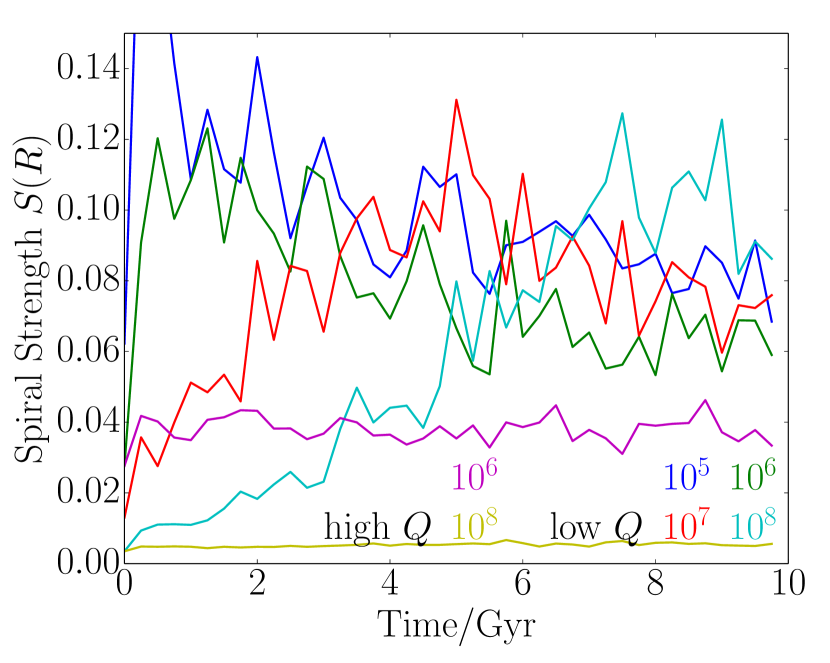
Figure 1: The growth of transient spiral structures with time for discs with $10^{5}$, $10^{6}$, $10^{7}$ and $10^{8}$ particles. Spiral strength $S(R)$ is defined in equations (9) and (10), where all $m\leq 12$ modes are taken into account. Spiral structures grow in all four low-$Q$ discs, but not in high-$Q$ discs. For the high-$Q$ disc with $10^{6}$ particles, the strength is higher than that of $10^{8}$ particles due to higher Poisson noise, but does not grow over time. The scale time for growing spirals is longer for simulations with more star particles. For simulation with $10^{5}$–$10^{7}$ star particles, spiral strength decreases after reaching the peak value due to the spiral heating.

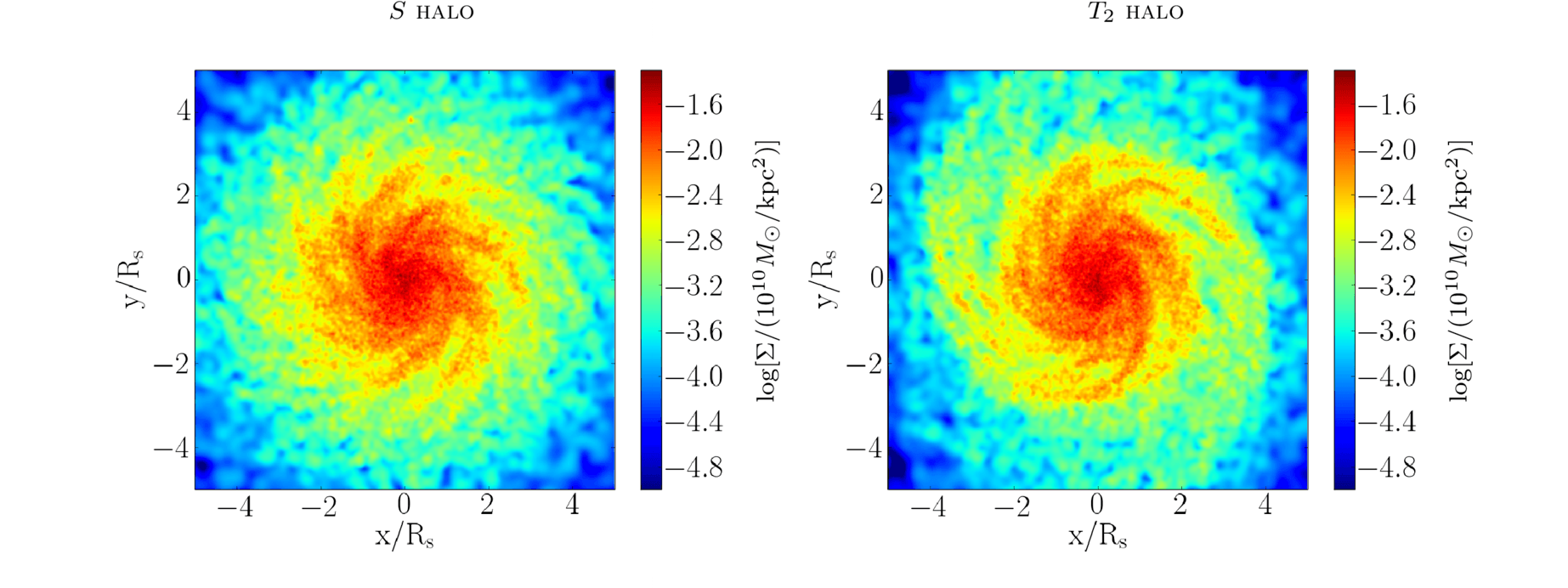
Figure 2: Surface density of a disc in the spherical and the $T_{1}$ triaxial halo at time $0.5\mathrm{Gyr}$. Values on the colour bar are $\mathrm{log}(\Sigma/10^{10}\mathrm{M}_{\rm\odot}\mathrm{kpc}^{-2})$, where $\Sigma$ is the surface density. In both simulations the disc has $10^{5}$ particles. The surface densities of the two discs are similar. This indicates that when the Poisson noise is significant, swing amplification of Poisson shot noise is the dominating factor over the influence of a triaxial halo.

In simulations with low-$Q$ discs, transient spiral structures develop. As shown in Fig. 17 in Appendix A, these spiral structures are multi-armed, typically from 7-armed to 10-armed. The strength of these spiral structures at radius $R$ can be quantified with

$$$S(R)$=\sqrt{\sum_{m=1}^{12}\left|\frac{\hat{\Sigma}_{m}(R)}{\hat{\Sigma}_{0}(R)}\right|^{2}}\,,$$ (9)

where $\hat{\Sigma}_{m}(R)$ is the Fourier transformation of the surface density $\Sigma(R,\theta)$ of the disc at fixed radius $R$ along the azimuthal coordinate $\theta$, i.e.

$$\hat{\Sigma}_{m}(R)=\frac{1}{2\uppi}\int_{\mathrm{-\uppi}}^{\uppi}\Sigma(R,\theta)\mathrm{e}^{-\mathrm{i}m\theta}\mathrm{d}\theta\,.$$ (10)

Here we sum over $m=1$–$12$ to include the effect of all spiral structures with $m\leq 12$. Structures with higher $m$, which represent smaller structures in the disc, are excluded because they are subject to random noise in the disc. The evolution of $S(R)$ over a time span of $10\,\mathrm{Gyr}$ at a fixed radius $R=2R_{\mathrm{S}}$ is shown in Fig. 1.

Strong spiral structures develop in all four simulations with low-$Q$ discs. The maximum spiral strength for these simulations is roughly the same regardless of the number of star particles. However, simulations with a higher number of particles take longer time to grow spiral structures, in agreement with the findings from Sellwood (2012) and Fujii et al. (2011). This shows that self-gravitating discrete discs in our simulation can be well characterized by Balescu–Lenard equation, whereby the time-scale of structure growth is inversely proportional to the number of particles in the system (Fouvry et al., 2015). In particular, it takes more than $7\mathrm{Gyr}$ for the simulation with $10^{8}$ star particles to fully develop spiral structures. Also note that spiral strength in simulations with $10^{5}$–$10^{7}$ particles decreases after reaching the maximum, because of spiral heating. For ‘dynamically hot’ discs with $Q>1.3$, the spiral strength is always comparable to the initial value, indicating that the swing amplification is weak, as expected.

To further study the resolution effects, we replace the spherical halo with triaxial haloes described in Table 2. Fig. 2 shows the surface density of a $10^{5}$ particle disc in the $T_{1}$ halo at time $t=0.5\,\mathrm{Gyr}$. $T_{1}$ halo is triaxial inside and spherical outside, which means that the non-axisymmetric force introduced by this halo in the central region of the disc is very high. However, the disc in the $T_{1}$ halo still develops a multi-armed transient spiral structure, though the distribution of the spiral arms is more asymmetric than the one in the spherical halo. This indicates that when the Poisson noise in the disc is very high, swing amplification of the disc dominates the whole process and external torques cannot significantly influence the strength of the arms. To study carefully the effects of triaxial haloes, swing amplification of Poisson noise caused by finite resolution needs to be suppressed. For the rest of this paper, we thus perform simulations with $10^{8}$ star particles, so that the growth of transient spiral structures caused by swing amplification of the Poisson noise in the initial conditions is sufficiently slow.

3.2 Time-dependent Triaxial Haloes

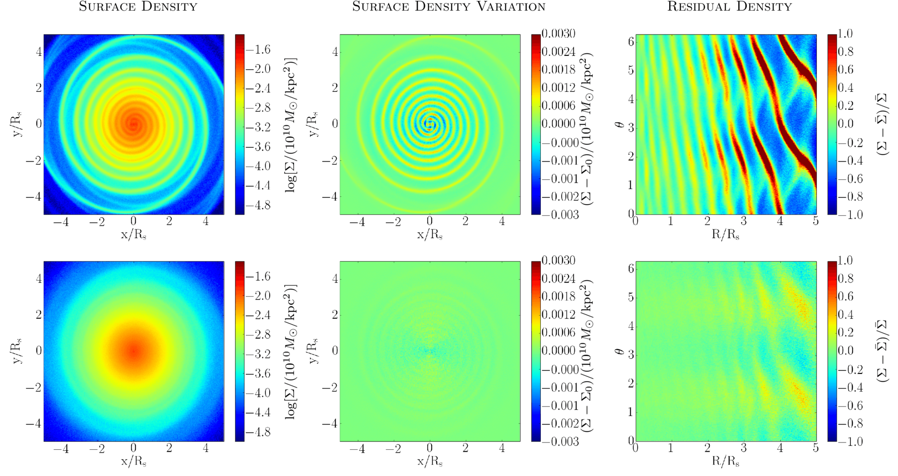
Figure 3: Surface density, i.e. $\mathrm{log}(\Sigma/10^{10}\mathrm{M}_{\rm\odot}\mathrm{kpc}^{-2})$, its variation to the initial conditions and residual density of high-$Q$ discs in a simulation with $10^{8}$ star particles in a $T_{2}$ halo at $t=3\mathrm{Gyr}$. Top row: simulation with a static $T_{2}$ halo. Bottom row: halo is initially spherical and then gradually turns into a $T_{2}$ halo with a scale time of $\tau=1\mathrm{Gyr}$. In the simulation with a static $T_{2}$ halo, strong two-armed spiral structures form. The spiral structures keep winding up after their formation. By the time $t=3\mathrm{Gyr}$, spirals are tightly wound up. With triaxiality of the halo introduced gradually, very weak spiral structures form in the disc, indicating that the spiral structures found in the simulation with a static triaxial halo are caused by the sudden change of the halo shape.

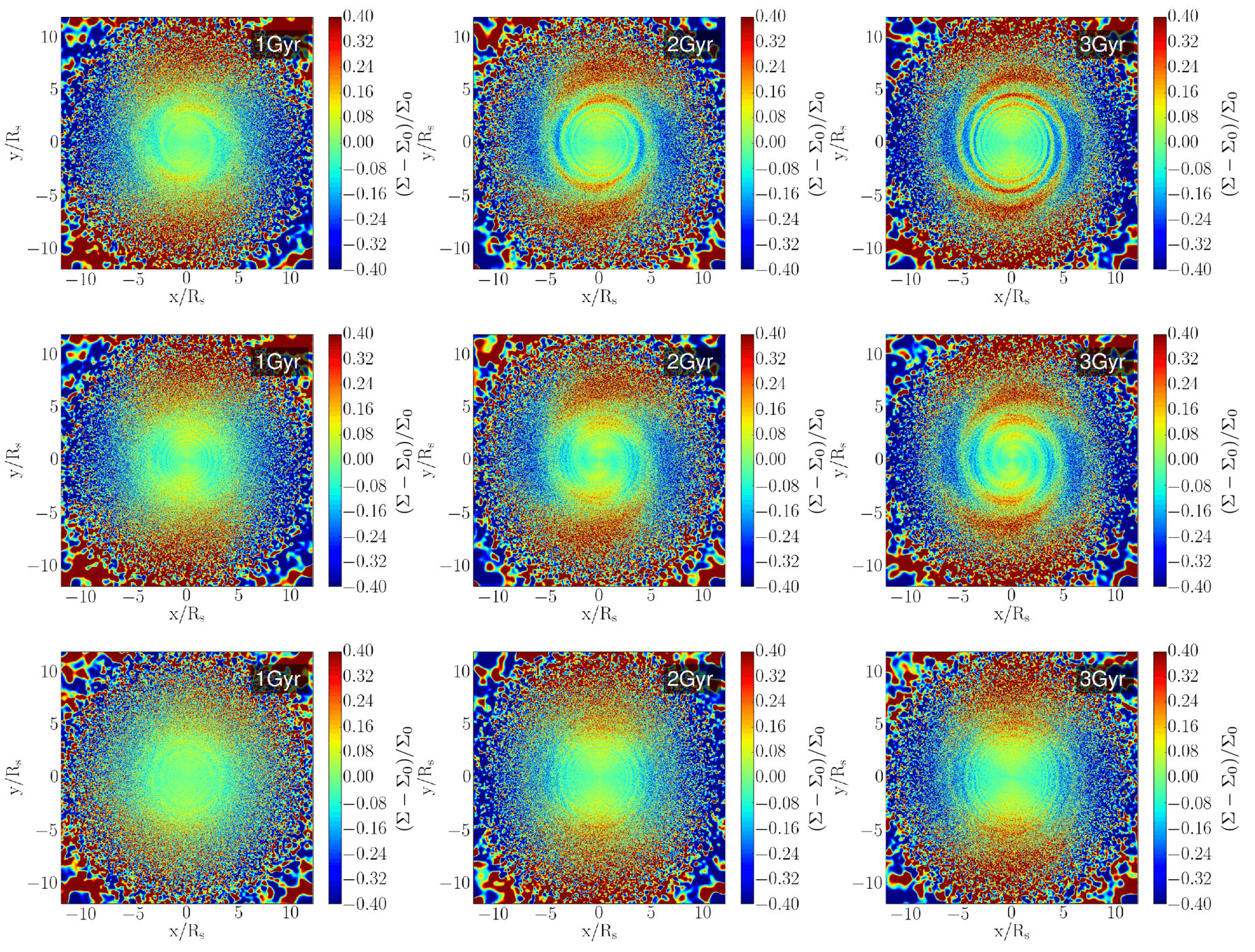
Figure 4: Discs in a $T_{2}$ halo with a gradually increasing triaxiality with time. The relative difference of surface density to the initial conditions is shown. Top: with self-gravity. Middle: without self-gravity. Bottom: with self-gravity and a smoother introduction of triaxiality in the halo, i.e. $f_{6}(t)$ as defined in equation (15). With self-gravity in the disc turned off, it can be clearly seen that a two-armed spiral structure forms outside and grows inwards. However, for the simulation with self-gravity, this spiral pattern interferes with rings that form due to the change of halo profile. When the triaxiality of the halo is introduced in a smoother way, no prominent spiral structures can be found. This indicates that discs can survive in triaxial haloes without developing spiral structures if the shape of the halo changes smoothly enough.

The top row of Fig. 3 shows the surface density, density variation with respect to the initial conditions and the residual density of the high-$Q$ disc with $10^{8}$ star particles in the $T_{2}$ halo at $3\mathrm{Gyr}$. Here residual density refers to the normalized density difference to the average surface density over azimuthal coordinate,

$$\Sigma_{\mathrm{res}}(R,\phi)=\frac{\Sigma(R,\phi)-\bar{\Sigma}(R)}{\bar{\Sigma}(R)}\,,$$ (11)

where $\bar{\Sigma}(R)$ is the average density at radius $R$, i.e. $\bar{\Sigma}(R)=\frac{1}{2\uppi}\int_{0}^{2\uppi}\Sigma(R,\phi)\mathrm{d}\phi$. We use a high-$Q$ disc to avoid the possible interference due to the swing amplification of the disc, which we study later on in Section 3.5. As shown in the top row of Fig. 3 strong grand-design two-armed spiral structures form. These spiral structures are very sharp, tightly wound up and global. Unlike the spiral structures formed due to swing amplification (see Fig. 17), which only exist in the intermediate part of the disc (i.e. for $1\lesssim R/R_{\mathrm{S}}\lesssim 3.5$), the spiral structures in triaxial halo extend to the edge of the disc. This agrees with Dubinski & Chakrabarty (2009) where an external torque due to the tumbling dark matter halo drives the formation of the spiral structures. However, it is unclear whether these spiral structures are caused by the triaxial halo alone or by the impulsive process of introducing triaxial haloes to the system with a disc that is initially in equilibrium with a spherical halo.

To fully understand the formation mechanism of these grand-design spiral structures, we run simulations in which the shape of the halo changes from spherical to triaxial gradually, so that initially the disc is in the equilibrium with the halo and no impulsive change to the system occurs. As shown in equations (6) and (7), the analytic potential we employed in our simulations consists of two parts: a spherical Hernquist potential and a triaxial part. We hereby extend equation (6) so that the triaxial part of the halo can be turned on and off gradually with a function $f(t)$,

$$\Phi(r,\theta,\phi)=\Phi_{\rm HQ}(r,\theta,\phi)+f(t)\Phi_{\rm T}(r,\theta,\phi)\,.$$ (12)

When $f(t)=0$, the dark matter halo is a purely spherical Hernquist halo, while when $f(t)=1$, the dark matter halo is a fully developed triaxial halo.

The bottom row of Fig. 3 shows the surface density and the residual density of a simulation with a gradually introduced $T_{2}$ halo. In this simulation the growth of the triaxial part of the potential is set to

$$f(t)=1-\exp(-t/\tau_{\rm I})\,,$$ (13)

where the scale time $\tau_{\mathrm{I}}=1\mathrm{Gyr}$. The time shown in Fig. 3 is $3\mathrm{Gyr}$, when the triaxial transformation of the halo is almost complete, with $f=0.95$. With the initially spherical halo growing slowly to triaxial, as shown in the residual density map in the rightmost panel, the spiral structure is very weak inside $3R_{\mathrm{S}}$, while relatively weak two-armed structures develop in the outer region.

The fact that only weak spiral structures develop when the triaxiality of the halo is introduced gradually indicates that triaxial halo alone does not necessarily lead to spiral structures. In fact, by comparing the orbital period $\tau_{\mathrm{O}}$ of the stars and the time-scale $\tau_{\mathrm{I}}$ of introducing the halo, we find that the time-scales of the two processes determine whether a strong spiral structure will develop. The orbital period $\tau_{\mathrm{O}}$ is very small in the innermost regions of the disc. The introduction of triaxiality has a much longer time-scale $\tau_{\mathrm{I}}=1\mathrm{Gyr}$, which can be seen as an adiabatic perturbation in the centre. $\tau_{\mathrm{O}}$ becomes longer at larger radii. At $R=3R_{\mathrm{S}}$, $\tau_{\mathrm{O}}=0.315\mathrm{Gyr}$, which is still shorter than the $\tau_{\mathrm{I}}$, but the introduction of the halo is starting to make an effect. At about $R=5R_{\mathrm{S}}$, $\tau_{\mathrm{O}}\sim 0.5\mathrm{Gyr}$. Now introduction of the triaxial halo can no longer be considered as adiabatic, and the change of halo shape starts to have a significant effect on the disc.

The spiral structures formed in this simulation on larger scales are shown in the first row of Fig. 4. Here the normalized density difference to the initial density

$$\overline{\Delta\Sigma}=\frac{\Sigma-\Sigma|_{t=0}}{\Sigma|_{t=0}}$$ (14)

is shown so that the structures in outer regions where density is significantly lower can be clearly seen. As shown in different columns (which are for $t=1,2$ and $3\,\mathrm{Gyr}$), structures form at larger radii and grow inwards. However, due to the changing of the halo potential, ring structures also form in the disc and to a certain extent interfere with the spiral structures, making it hard to distinguish genuine spiral structures from rings. We therefore run another simulation with self-gravity in the disc turned off, as shown in the middle row of Fig. 4. Two-armed grand-design spiral structures still form in this simulation, but rings do not interfere with spirals through self-gravity anymore. Instead, they superimpose with each other so that the rings are now seen as fine lines in each arm of the spiral structures. We therefore conclude that rings, though forming easily as a response to the change of the halo potential and modifying the shape of the spiral structures, are not essential for the spiral forming process.

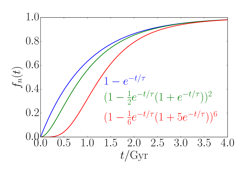
Figure 5: Time dependence of $f_{n}(t)$ for smoothing factor $n=1,2$ and $6$. $f_{n}(t)$ shows the same trend as $f_{0}(t)$ as $t\rightarrow\infty$. However higher $n$ indicates a smoother growth of $f_{n}$ at the beginning of the simulation.

We explore this problem further with a smoother $f(t)$ function. We generalized equation (13) to

$$f_{n}(t)=(1-\frac{1}{n}\mathrm{e}^{-t/\tau_{\mathrm{I}}}(1+(n-1)\mathrm{e}^{-t/\tau_{\mathrm{I}}}))^{n}\,,$$ (15)

where $n$ is the smoothing factor and $f_{1}(t)$ falls to the original form used in equation (13). This generalization satisfies $f_{n}(0)=0$ and $f_{n}(t)=f_{1}(t)$ to the first order in $\mathrm{e}^{-t/\tau_{\mathrm{I}}}$ as $t\rightarrow\infty$. As shown in Fig. 5, for a higher $n$, the growth of $f(t)$ at the early stage of the simulation is smoother. In practice we ran a simulation with $n=6$. Self-gravity is included in this simulation as well. The result of this simulation is shown in the bottom row of Fig. 4. No prominent spiral structures develop. This demonstrates that the triaxial shape of a halo itself does not necessarily lead to spiral structures. Rather, non-adiabatic change of the halo shape, i.e. halo changing on a time-scale shorter than or comparable to the orbital period of the stars, will cause grand-design spiral structures to form.

Khoperskov et al. (2013) have reported that in their simulations similar grand-design two-armed spiral structures form within a halo growing slowly enough from a spherical one to a triaxial one with a time-scale more than four times longer than the rotation periods of the stars at the outer part of the disc. In contrast, we have shown in Fig. 4 that with a carefully chosen growth function $f(t)$ of the triaxiality of the halo, the development of the spiral patterns is not necessary. We therefore conclude that the spiral structures formed in their simulations are also due to the fact that the introduction of the triaxiality is not adiabatic enough.

As also shown in the bottom row of Fig. 4, when the change of halo shape is adiabatic enough, the most prominent feature of the disc is its ellipticity. It has been shown that the ellipticity of the potential in the disc plane as well as the ellipticity of the disc itself can be constrained by the scatter of Tully–Fisher relation and by the photometry (Franx & de Zeeuw, 1992; Debattista et al., 2008). The potential ellipticity is defined as $\epsilon=b_{\Phi}/a_{\Phi}$ where $a_{\Phi}$ and $b_{\Phi}$ are the length of major and minor axis of the surface of a constant potential. In our $T_{2}$ model, it varies from $\epsilon=0.055$ to $0.075$ in the disc plane from the inside to the outside. The ellipticity of the disc, defined similarly by contours of disc surface density, is $\epsilon_{\mathrm{D}}=0.05$. Both of the ellipticities are consistent with $\epsilon<0.1$ and $\epsilon_{D}=0.06$ as suggested by Franx & de Zeeuw (1992).

To understand if triaxial haloes are needed for these grand-design spiral structures to survive for longer periods of time, we also run a simulation with the halo shape turning from triaxial to spherical abruptly, with

$$f(t)=\exp(-(t/\tau_{\rm D})^{2})\,,$$ (16)

with a time-scale $\tau_{\rm D}=0.2\mathrm{Gyr}$. In this simulation strong spiral structures form at the beginning of the simulation almost instantly, as expected. We run simulation further in time and find that the spiral structures can persist for much longer time. The surface density, its variation to the initial conditions and the residual density of the disc at $t=3\mathrm{Gyr}$ are shown in Fig. 6. The halo is extremely close to spherical as early as $t=0.5\,\mathrm{Gyr}$, with $f\sim 10^{-3}$. Spiral structures survive in this spherical halo for at least $2\mathrm{Gyr}$ and remain strong. Therefore, triaxial haloes, proven above not necessary for forming spiral structures, are not needed for persisting spiral structures either.

It is interesting to note that Toomre (1981) studied properties of a disc galaxy with an external torque turned on and off rapidly. Though both in Toomre’s and in our simulations, two-armed spiral structures form, they are different in at least two ways. First, in Toomre (1981), the Toomre’s $Q$ parameter and the wavelength ratio $X$ are both in the range that favours the swing amplification of $m=2$ modes, while in our simulation, for $m=2$ the wavelength ratio $X$ is too high for swing amplification to become significant. Actually in our simulations the modes for the $X$ to fall into the range $1<X<3$ that favours the swing amplification require $7\lesssim m\lesssim 10$, which are the typical number of arms for transient spiral structures seen in Fig. 17. Therefore, though the swing amplification plays an important role in the development of the grand-design spiral structures in Toomre (1981), it plays a minor role in our simulations. In fact, as shown later in Section 3.5, the swing amplification may destroy the grand-design spiral structures at later times. Secondly, Toomre (1981) found that the grand-design spiral structures in their simulation decay after several rotational periods, while in our simulations the grand-design spiral structures can survive for a longer time. While disc properties and simulation methodology in our work are quite different, this indicates that the formation mechanism of the spiral structures may be different in Toomre (1981) and our simulations. In fact, the spiral structures in our simulations can be well explained by the kinematic density wave theory, as shown in Section 3.5.

3.3 Time-dependent Triaxial Haloes from Cosmological Simulations

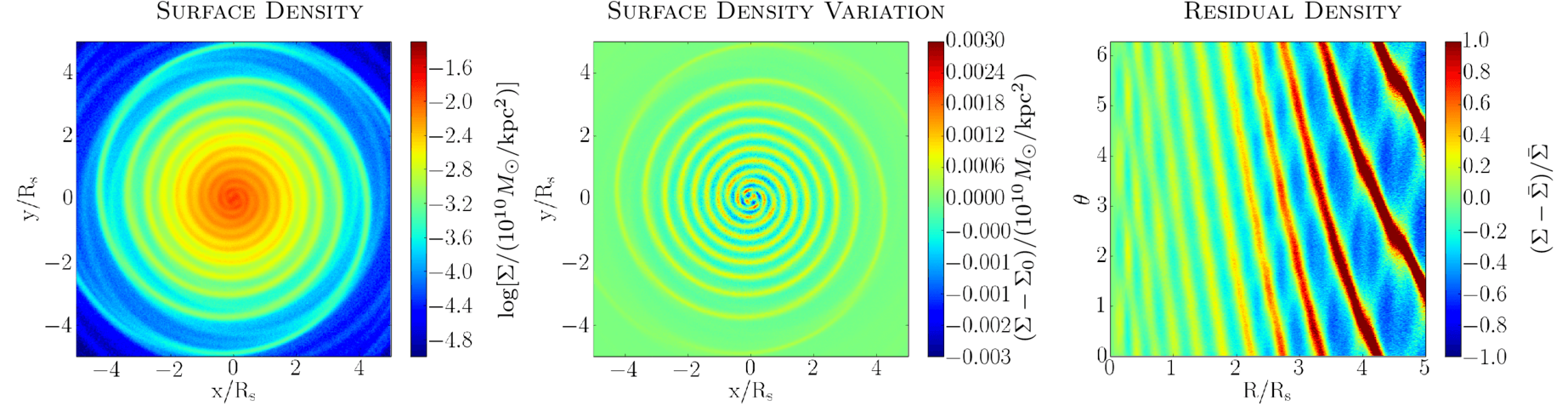
Figure 6: Simulated discs at $t=3\,\mathrm{Gyr}$ in a halo that has a time-dependent triaxiality. Halo starts as the $T_{2}$ halo, but is quickly turned into a spherical halo with a scale time of $\tau=0.2\mathrm{Gyr}$. The grand-design spiral structures still exist for a long time, indicating that once formed, grand-design spiral patterns can survive in a spherical halo.

Triaxiality Profile of the First Model

Triaxiality Profile of the Second Model

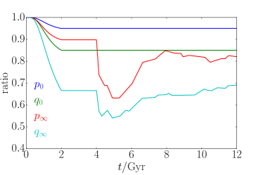
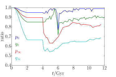
Figure 7: Time dependence of the major axial ratios of the halo isodensity surface. For both models, from 0 to $2\,\mathrm{Gyr}$, the halo grows from spherical to triaxial smoothly. At $2\,\mathrm{Gyr}$, the triaxiality of the outer halo is the same as that of the Aq-B-4 halo at $5.4\,\mathrm{Gyr}$ of the original simulation, as shown in fig. 5 of Vera-Ciro et al. (2011). The halo is kept static until $4\,\mathrm{Gyr}$, allowing the disc to fully relax. From $4\,\mathrm{Gyr}$, the outer side of the halo evolves similarly to the Aq-B-4 halo starting from $5.4\,\mathrm{Gyr}$ in the Aquarius simulation, while the limits of the major axial ratios as $r\rightarrow 0$ remain constant for the first model (left-hand panel), but evolve following a recalibration based on the Aq-B-4 simulation for the second model (right-hand panel).

As shown in the previous section, spiral structures only form when the axisymmetric change of halo potential is rapid enough. It is natural to ask whether this process is possible in a realistic halo. In fact, Vera-Ciro et al. (2011) found that haloes in self-consistent cosmological simulations like the Aquarius runs (Springel et al., 2008) can have very rapid change in triaxiality over time even when not experiencing very violent major mergers. To directly explore the impact of such realistic triaxiality changes on stellar discs, we set up two isolated halo models. For both models, the axial ratios $p=b/a$ and $q=c/a$ at the outer side of the halo follow Aquarius halo Aq-B-4 [see fig. 5 in Vera-Ciro et al. (2011) at $\sim 5.4\,\mathrm{Gyr}$ of their simulated time]. The first model we consider has constant axial ratios with time in the central region. The limit of triaxiality as $r\rightarrow 0$ is set to be $p_{0}=b/a|_{r\rightarrow 0}=0.95$ and $q_{0}=c/a|_{r\rightarrow 0}=0.85$ similar to the $T_{2}$ model (following Zemp et al., 2012), to account for the likely impact of baryonic matter.

This model is rather conservative as it does not account for any time variation of triaxiality in the innermost halo regions. Thus, for the second model, we directly calculate the time evolution of the inner triaxiality of the Aq-B-4 halo. Due to the possible influence of a baryonic component, which is not captured by the Aquarius simulation (as it contains dark matter only), we expect that the average inner triaxiality will be smaller, but that the time fluctuations of triaxiality triggered by mergers, for example, will be comparable as predicted by dark matter-only cosmological simulations. We hence impose inner halo triaxiality fluctuations as directly evaluated from the Aq-B-4 halo on top of more realistic $p_{0}=b/a|_{r\rightarrow 0}=0.95$ and $q_{0}=c/a|_{r\rightarrow 0}=0.85$ values, rather than taking the absolute Aq-B-4 inner triaxiality average values, which are in the range of $\sim 0.6$. With this “recalibration” our second model more closely reflects the possible inner triaxiality time evolution as would be obtained by very high resolution Aq-B-4 simulation which would include baryons. Thus the impact of halo triaxiality on the stellar disc should be more realistic than in our first model.

The time dependence of halo triaxiality of our models is shown in Fig. 7. We start from a spherical halo and change the triaxiality of the halo adiabatically to the configuration resembling the Aq-B-4 halo at $5.4\,\mathrm{Gyr}$ of the original simulation, and let the disc relax for $2\,\mathrm{Gyr}$ before the outer halo triaxiality starts to evolve similarly to the Aq-B-4 halo onwards in time. In the left-hand panel of Fig. 7 we show our first model where the inner halo triaxiality is kept constant, while in the right-hand panel, corresponding to our second model, realistic cosmological fluctuations of inner halo triaxiality are imposed (as measured from the Aq-B-4 simulation directly) on top of the same constant values as in the first model.

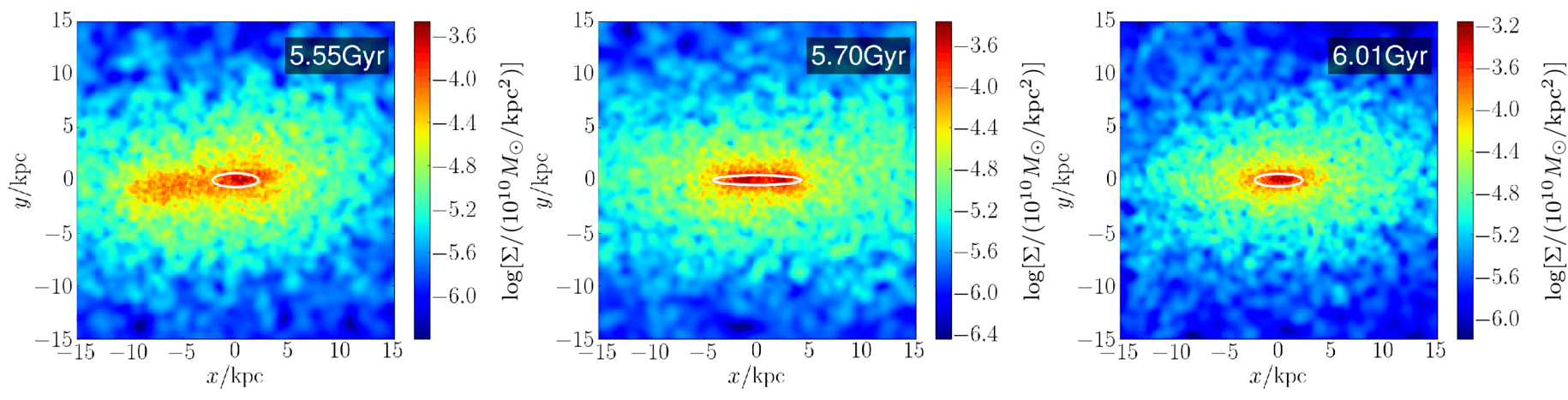
Figure 8: Time sequence of the central Aq-B-4 halo from $5.55$ to $6.01\,\mathrm{Gyr}$. The panels show the projected density of the dark matter halo. White ellipse represents the fit to the halo shape at $\sqrt[3]{abc}=1\,\mathrm{kpc}$, where $a,b$ and $c$ are the lengths of the three axes. A satellite merges with the Aq-B-4 halo during this period, which leads to a temporary but abrupt halo shape change.

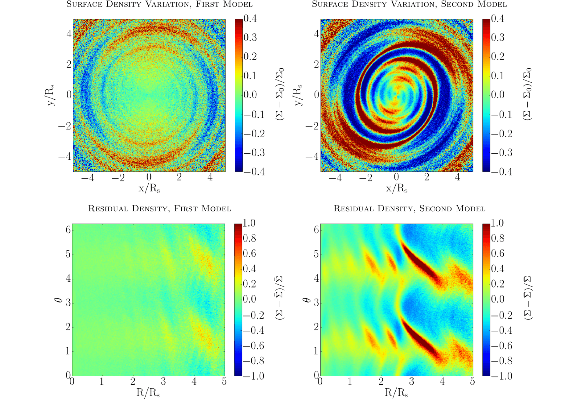
Figure 9: Surface density difference to the initial conditions (top) and residual densities (bottom) at $t=6\,\mathrm{Gyr}$ of discs evolved in simulations shown in Fig. 7. The halo starts to behave like Aq-B-4 halo after $t=4\,\mathrm{Gyr}$ in this simulation. At $t=6\,\mathrm{Gyr}$, clear spiral structures already develop for both simulations, while for the second model with varying inner triaxiality, the spiral strength is larger, and spirals form further in.

Ratio of Major Axes

Torque Strength

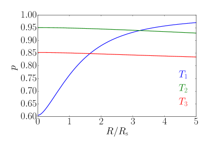
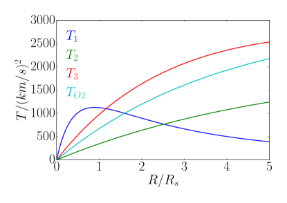
Figure 10: Shape and torque strength of the dark matter halo models as a function of $R/R_{\mathrm{S}}$. Left: ratio of major axes, $p=b/a$, as a function of $R/R_{\mathrm{S}}$ for halo models $T_{1}$, $T_{2}$ and $T_{3}$ listed in Table 2. Right: absolute value of the torque perpendicular to the disc plane that a star with azimuthal coordinate $\theta=\uppi/4$ and radius $R$ feels for simulations with halo models $T_{1}$, $T_{2}$, $T_{3}$ and $T_{\mathrm{O2}}$. The simulation with halo model $T_{\mathrm{O2}}$ is discussed later in Appendix B.

A prominent feature in the right-hand panel of Fig. 7 is a sharp dip at around $6\,\mathrm{Gyr}$. A minor merger is found to be the cause for such a sharp change, as illustrated in Fig. 8. We trace this merger event backwards in time, and find that the satellite that causes this merger event has initially $\sim 23\%$ of the mass of the Aq-B-4 halo. As it inspirals towards the centre of the Aq-B-4 halo, which lasts for about $3\,\mathrm{Gyr}$, it loses most of its mass gradually due to dynamical friction and tidal stripping. None the less, the core of the satellite disrupts the centre of the Aq-B-4 halo significantly as it finally merges with it.

For both models, as intended the disc shows no sign of spiral structures in the growing and relaxing phase over the first $4\,\mathrm{Gyr}$. However, when our halo triaxiality starts to evolve like that of the Aq-B-4 halo, clear spiral structures form in about $2\,\mathrm{Gyr}$, as shown in Fig. 9. The spiral structures persist and sharpen over time for at least another $3$–$4\,\mathrm{Gyr}$. The morphology of the spiral structures is very similar to those shown in Section 3.2. Generally, the spiral structures of the second model with changing inner triaxiality are much stronger than that of the first model. Also, for the second model the spiral strength is high all through the disc, while for the first model, the spiral structures are stronger in the outer part of the disc, which is expected since the inner limit of triaxiality is fixed. None the less, the spiral strength of the first model is still considerable as the relative surface density fluctuations reach $40\%$. We therefore conclude that in a realistic, cosmologically motivated case, changes in the halo triaxiality are abrupt enough to cause spiral structures, even when we assume a conservative evolution for the innermost halo. In reality, due to minor mergers, the inner shape of the halo may change in a way similar to our second model, therefore leading to strong spiral structures similar to the right-hand panels of Fig. 9. More detailed investigation of this issue, which depends on the complex interplay of baryons and inner halo triaxiality fluctuations with time is beyond the scope of this work and is left for a future study.

It is also possible that in reality the disc is misaligned with respect to the halo’s major plane. We explore this in Appendix B and find that the misaligned disc no longer stays in a plane as it evolves. Integral shaped warps form in the disc. Two-armed spiral structures still form and are similar to those formed in discs that lie in the $x$–$y$ plane of the triaxial haloes. However, the outer parts of the spiral structure are distorted, due to the fact that they are no longer in the disc plane.

3.4 Dependence of Spiral Strength on the Halo Shape

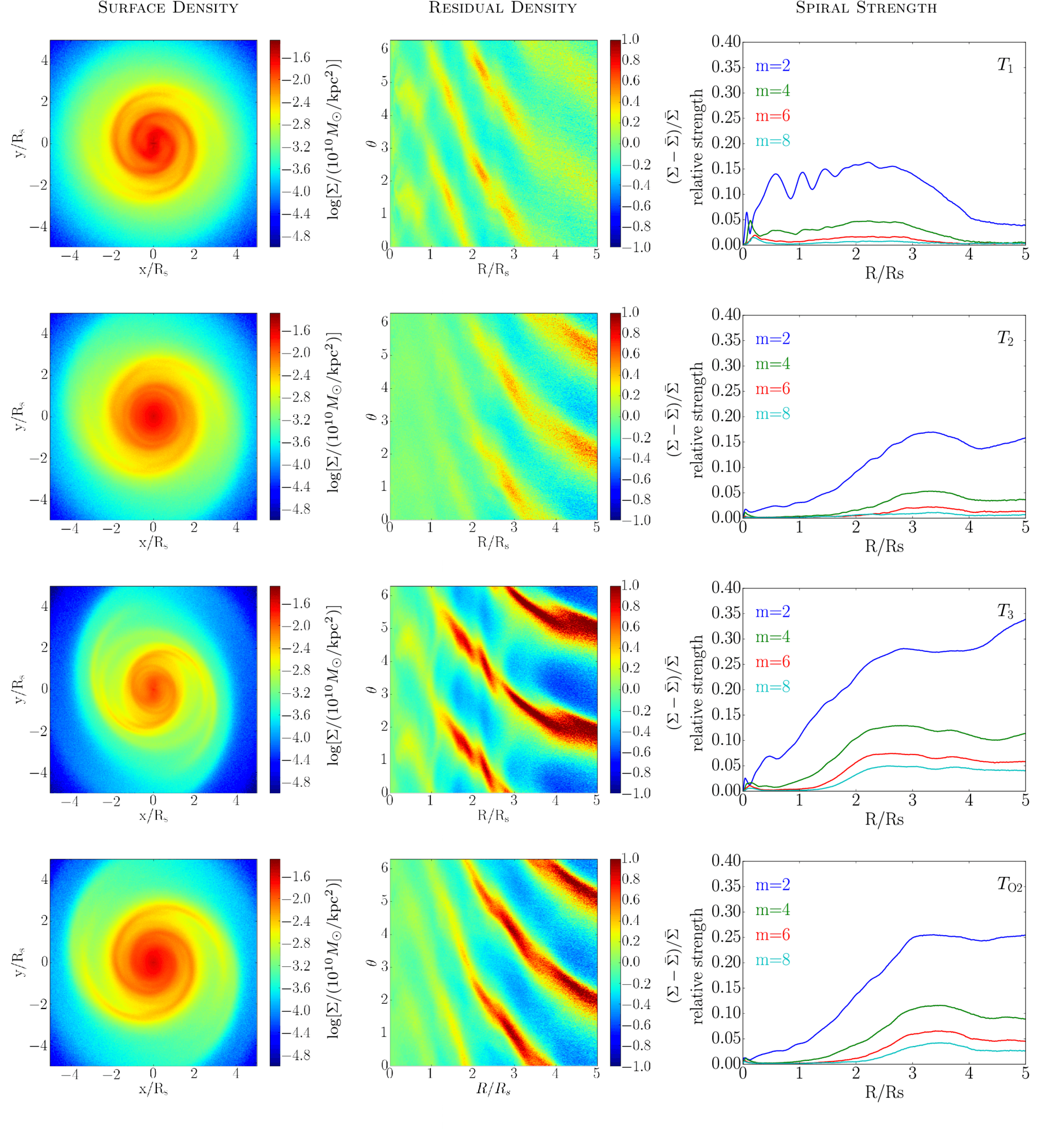
Figure 11: Surface density, residual density and spiral structure strength of discs in simulations with $T_{1}$, $T_{2}$, $T_{3}$ and $T_{\mathrm{O2}}$ haloes (from top to bottom). Left column: surface density in Cartesian coordinates at time $t=0.5\,\mathrm{Gyr}$. Central column: residual density in polar coordinates at time $t=0.5\,\mathrm{Gyr}$. Right column: spiral strength for different modes averaged over a time interval from $0.35$ to $0.85\,\mathrm{Gyr}$. This time interval in chosen so that the spiral structures are fully developed in the disc. Note that spiral strengths with the odd $m$ modes are not shown because they are much weaker. For the halo that is more triaxial inside ($T_{1}$), the spiral structure is stronger inside, while for the halo that is more triaxial outside ($T_{2}$), the spiral structure is also stronger outside. For $T_{3}$ halo which has $b/a\sim c/a\sim 0.85$, the spiral structure strength is generally higher than the other two simulations, expect for the central region where the spiral structure strength is lower than that of the $T_{1}$ halo. For the $T_{\mathrm{O2}}$ halo, the disc plane is determined by the direction of the total angular momentum, as discussed later in Appendix B.

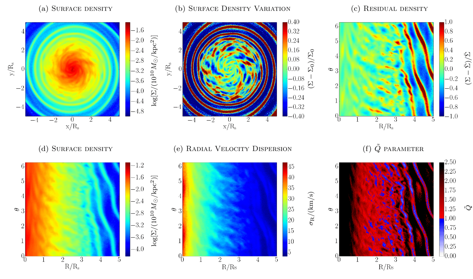
Figure 12: Maps of various quantities of a low-$Q$ stellar disc in the $T_{2}$ halo at time $3\,\mathrm{Gyr}$. Panel (a) shows the surface density in Cartesian coordinates. To show the structures throughout the disc more clearly, we subtracted the initial surface density $\Sigma_{0}$ from the surface density $\Sigma$ at $3\mathrm{Gyr}$ and then divided it by $\Sigma_{0}$. The result is shown in panel (b). Panel (c) shows the residual density map in polar coordinates. In panel (d), (e) and (f), surface density, dispersion of the velocity in the radial direction, $\sigma_{\mathrm{R}}$, and $\tilde{Q}$ parameter are shown in polar coordinates. Here $\tilde{Q}(R,\theta)=\frac{\sigma_{R}\kappa}{3.36\,G\Sigma}$. Toomre’s $Q$ parameter is the angular average of $\tilde{Q}$. $\tilde{Q}$ quantifies the local stability of the disc. Two different types of spiral structures co-exist in the disc. Outside $3.5R_{\mathrm{S}}$ is the grand-design two-armed spiral structure caused by the triaxial halo, while inside $3.5R_{\mathrm{S}}$ there are more arms and they are all transient.

We performed three additional simulations to further study the influence of different halo shapes on the spiral structure strength. In these simulations, we employ low-$Q$ discs and various static triaxial dark matter haloes. The disc is originally in equilibrium with a spherical halo. An abrupt introduction of the triaxiality in the halo is the cause of spiral structures, as shown in Section 3.2.

Three halo models, $T_{1}$, $T_{2}$ and $T_{3}$, introduced in Table 2, are used in these simulations. The ratio of major axes, $p=b/a$, of these haloes at different radii is shown in the left-hand panel of Fig. 10. $T_{1}$ model is more triaxial inside, $T_{2}$ model is more triaxial outside, and the ratio of the major axis of the halo in the $T_{3}$ model is equal at the innermost and the outermost limits, and slightly lower in between. In all three simulations, spiral structures develop instantly in response to the abrupt change of the halo shape from the spherical one. Surface density $\Sigma$, residual density $\Sigma_{\mathrm{res}}$ and the relative spiral strength of different $m$ modes, $S_{m}$, of the discs in these simulations are shown in Fig. 11. Here the relative spiral strength $S_{m}$ is defined as

$$S_{m}(R)=\left|\hat{\Sigma}_{m}(R)/\hat{\Sigma}_{0}(R)\right|\,,$$ (17)

where $\hat{\Sigma}_{m}(R)$ is the Fourier transformation of the surface density of the disc at radius $R$ along the azimuthal coordinate, as defined in equation (10). In practice, the spiral strength fluctuates over time at a given radius. To show the mean trend of the strength with respect to the radius, we therefore plot the averaged spiral strength over a time interval from $0.35$ to $0.85\,\mathrm{Gyr}$.

As shown in the top three rows of Fig. 11, two-armed spiral structures form in all three simulations. The spiral strength for $m=2,4,6$ and $8$ has a similar radial profile within each simulation, indicating that the spiral strength measured for higher $m$ modes is largely due to the two-armed spiral structures. However, for different simulations, the relative spiral strength, $S_{m}$, varies differently with radius $R$. Generally, spiral strength depends on the halo triaxiality. This can be understood by comparing the torque generated by the triaxial halo, as shown in the right-hand panel of Fig. 10. The torque and the strength of the spiral structures show almost identical trends as a function of radius for all three simulations, i.e. by comparing different simulations, one can find that the strength of the spiral structures at a given radius is higher for the simulation where the torque at that radius is stronger, and vice versa.

3.5 Swing Amplification of Spiral Fragments

As shown in Fig. 1, for a low-$Q$ disc with $10^{8}$ star particles located in a spherical halo, transient spiral structures develop in several $\mathrm{Gyr}$ due to swing amplification. To explore if this process will also take place in simulations with a triaxial halo, we run the simulation with a $T_{2}$ halo for a longer time.

As shown previously in Fig. 11, at first only two-armed spiral structures develop in the disc. However after some time transient multi-armed spiral structures gradually form in the central region of the disc. Various properties of the disc in this simulation at $t=3\,\mathrm{Gyr}$ are shown in Fig. 12. It can be seen from the surface density of the disc that two kinds of spiral structures co-exist in the disc, with transient spiral arm structures dominating the inner region of the disc, and two-armed grand-design spiral structures taking up the outer region.

Generally, the swing amplification is strong when the $Q$ parameter is close to unity. Fig. 12 shows that regions with low $\tilde{Q}(R,\theta)=\frac{\sigma_{R}\kappa}{3.36\,G\Sigma}$ value (note that Toomre’s $Q$ parameter is the angular average of $\tilde{Q}$) lie perfectly within the spiral structures. This indicates that the spiral arms, with their higher density, can attract more stars into the spiral arms, hence magnifying the strength of the spiral structures. Also, in the part of the disc with $R_{\mathrm{S}}<R<3.5R_{\mathrm{S}}$, the $\tilde{Q}$ parameter is generally slightly higher than $1$ outside of the spiral structures. This explains why transient spiral structures form in this region due to swing amplification, while for $R>3.5R_{\mathrm{S}}$ azimuthally averaged $\tilde{Q}$ value is significantly higher than $1$.

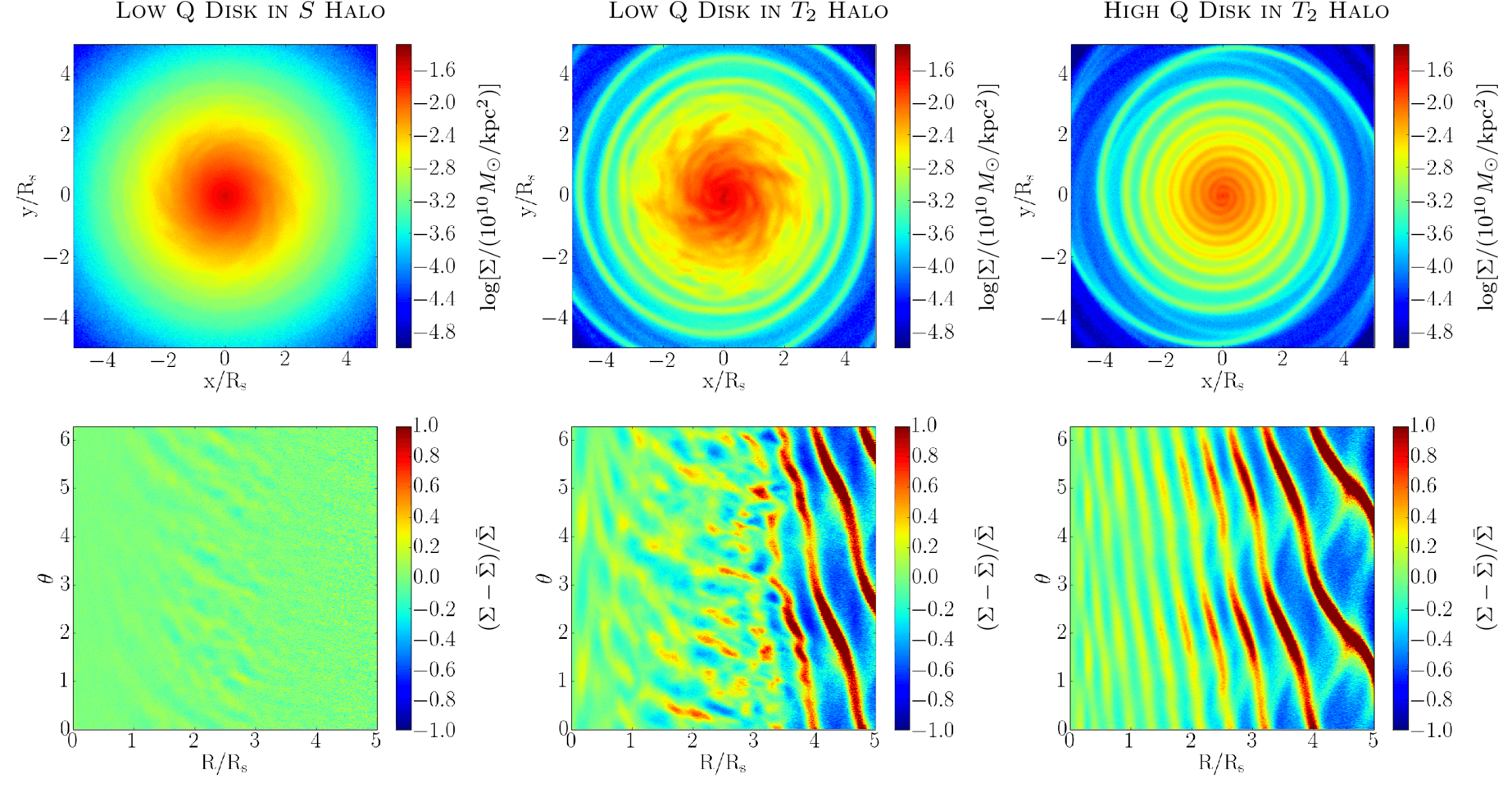
Figure 13: Surface density (top row) and residual density (bottom row) for discs in three different simulations at time $t=3\,\mathrm{Gyr}$. By comparing the left and the middle column we find that the strength of the transient spiral structures is stronger for the disc in a triaxial halo, although they are both formed due to swing amplification. As shown in the right column, transient multi-armed spiral structures do not form with a high-$Q$ disc.

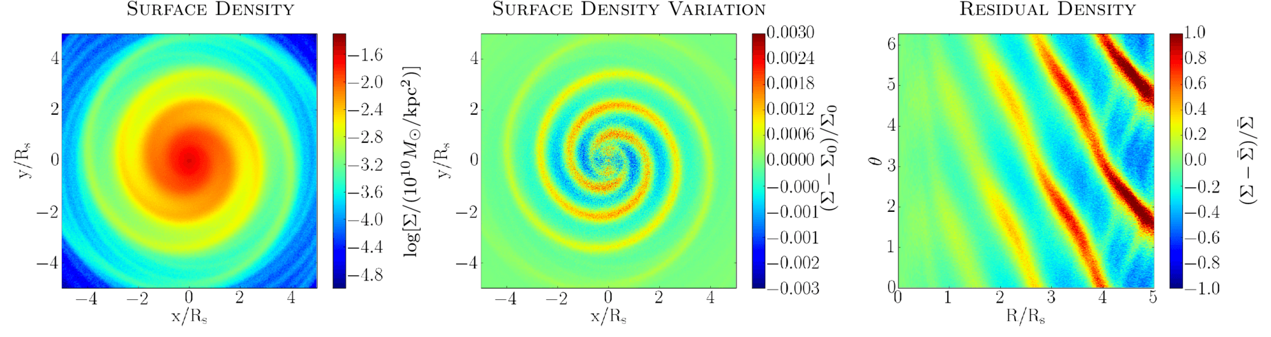
Figure 14: Simulation of low-$Q$ disc in $T_{2}$ halo without self-gravity at time $t=3\mathrm{Gyr}$. Without self-gravity, transient spiral structures no longer form, while the grand-design spiral structures still persist.

To further explore the interaction between grand-design spiral structures and swing amplification, we compare the discs formed in three different simulations: one with a low-$Q$ disc in a $T_{2}$ halo, one with a low-$Q$ disc in a spherical halo, and one with a high-$Q$ disc in a $T_{2}$ halo. The surface density and residual density of the discs in these simulations at $t=3\,\mathrm{Gyr}$ are shown in Fig. 13. By comparing the simulations with low-$Q$ and high-$Q$ disc in $T_{2}$ haloes, one can see that the transient arms do not form in the simulation with the high-$Q$ disc, where the swing amplification is very weak. This proves that the swing amplification is the reason for the formation of the transient spiral structures seen in the central regions of the low-$Q$ disc.

We additionally performed a simulation with self-gravity of the disc turned off with a low-$Q$ disc in a $T_{2}$ halo, whose result is shown in Fig. 14. No transient spiral structures form in this simulation, although two-armed grand-design spiral structures still form. Without self-gravity, there is no swing amplification process in the disc. This further demonstrates that transient arms are caused by the swing amplification, while two-armed grand-design spiral structures are not formed due to the swing amplification.

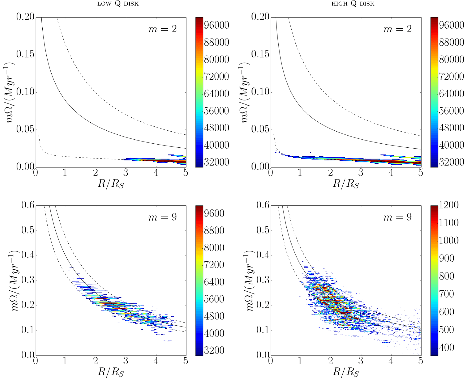
Figure 15: Power spectra of the low-$Q$ disc (left) and the high-$Q$ disc (right) for a time interval $2$–$7.5\,\mathrm{Gyr}$ in $T_{2}$ haloes for $m=2$ modes (top) and $m=9$ modes (bottom). In each panel, black solid curve indicates corotation line with pattern speed $\Omega_{\rm P}=\Omega$, where $\Omega$ is the angular velocity of the stars, while black dashed curves are inner and outer Lindblad resonances with $\Omega_{\rm P}=\Omega\pm\kappa/2$, with $\kappa$ being the epicyclic frequency. For $m=2$, the dominating feature corresponds to the grand-design spiral structures. For the low-$Q$ disc this structure only exists in the outer region, because the grand-design spiral structures are distorted by swing amplification. For the high-$Q$ disc where swing-amplification is weak, the grand-design spiral modes extend down to the innermost regions. The grand-design spiral structures lie at the inner Lindblad resonance. The dominating features of $m=9$ modes are the horizontal structures crossing the corotation line, which are the typical structures of swing amplified modes. The strength of these modes in high-$Q$ disc is roughly an order of magnitude lower than in the low-$Q$ disc, as can be seen from the colour bar. Other high-$m$ modes are not shown, as they are all qualitatively similar to the $m=9$ power spectra.

We also compare the simulations with low-$Q$ discs in $S$ and $T_{2}$ haloes as shown in Fig. 13. Transient spiral structures form in both cases. However, the transient spiral structures formed in the $T_{2}$ halo are significantly stronger than that formed in the $S$ halo. For the simulation with the $T_{2}$ halo, two-armed spiral structures formed in the central region of the disc at early times are gradually swing amplified and form the first generation of transient spiral structures later, while for the simulation with the $S$ halo, transient spiral structures form due to the swing amplification of the Poisson noise in the initial conditions. With $10^{8}$ particles in the disc, the Poisson noise is much weaker perturbation to the density field of the disc than grand-design spiral structures. Therefore, transient spiral structures formed in a $T_{2}$ halo are much stronger than that in an $S$ halo.

3.6 Formation Mechanism of Two-Armed Spiral Structures

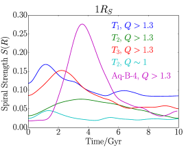
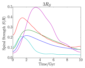
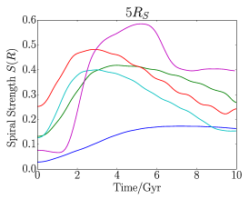
Figure 16: The strength of the $m=2$ spiral structures as a function of time for radii $R=1R_{\mathrm{S}},3R_{\mathrm{S}}$ and $5R_{\mathrm{S}}$ in various simulations. For simulations with $T_{1}$, $T_{2}$, and $T_{3}$, the halo is static and triaxial, while for the simulation with the Aq-B-4 halo (second model), the halo shape changes over time as in the right-hand panel of Fig. 7. For better comparison the time of the Aq-B-4 simulation has been shifted so that $t=0$ corresponds to $t=4\,\mathrm{Gyr}$ in Fig. 7. Curves have been smoothed with a Hann function over a $\sim 2\,\mathrm{Gyr}$ time span to show the general trends more clearly. For simulations with high-$Q$ discs, spiral strengths peak at $1$–$4\,\mathrm{Gyr}$ and then gradually decrease over several Gyr. In the $T_{2}$ halo with low-$Q$ disc the strength of grand-design spirals is affected by transient spirals after $1-2\,\mathrm{Gyr}$. Simulation with the Aq-B-4 halo shows stronger spiral strength due to its higher triaxiality and fluctuating evolution.

To understand the formation mechanism of two-armed spiral structures, we study the modes of spiral structures following Sellwood & Carlberg (2014), by measuring the power spectra of the discs in $T_{2}$ haloes. The surface density $\Sigma$ of the disc at time $t$, radius $R$ and azimuthal angle $\theta$ can be expressed by the summation of a series of waves

$$\Sigma(R,\theta,t)=\sum_{\Omega_{f}}\sum_{m}A(R,m,\Omega_{f})\mathrm{e}^{\mathrm{i}(\Omega_{f}t+m\theta)}\,,$$ (18)

where $m$ is the number of arms and $\Omega_{f}=m\Omega_{\mathrm{P}}$ is $m$ times the pattern speed $\Omega_{\mathrm{P}}$. In other words, $\Sigma$ is the Fourier transform of the power $A$. Values of $A(R,m,\Omega_{f})$ are complex numbers, as they are a combination of $\cos$ and $\sin$ waves. We are more interested in the absolute value $|A(R,m,\Omega_{f})|$, which is the total strength of the mode of $m$ and $\Omega_{f}$ at $R$. The power spectra are a good tool to study the waves in the disc, as they show the dominant rotational modes across the disc. In our simulations, since the surface density in the central region is much higher than that in the outer region, small fluctuations in the centre can have a higher power than the spiral structures located further out. In order to show the power spectra of the spirals clearly, we calculate power spectra of the residual surface density instead of the surface density.

Power spectra of low-$Q$ and high-$Q$ discs in $T_{2}$ haloes for a time interval from $2$ to $7.5\,\mathrm{Gyr}$ are shown in Fig. 15. For the power spectra of $m=2$ modes, the highest power lies at the inner Lindblad resonance where the pattern speed is $\Omega_{\mathrm{P}}=\Omega-\kappa/2$, with $\Omega$ being the rotation speed of the stars and $\kappa$ being the epicyclic frequency. Since the high power values occur within a narrow region across the disc, there is only one dominating rotating mode in the disc, with rotating speed of $\Omega-\kappa/2$. The high-power region in the power spectra of the $m=2$ modes of the high-$Q$ disc spans throughout the disc, but the high-power region for the low-$Q$ disc is located only at the outer region of the disc. This is because the inner region of the low-$Q$ disc is disrupted by the swing amplification, as previously shown in Fig. 13. We have also checked the $m=2$ power spectra of the simulation with self-gravity turned off. The high-power region lies at the inner Lindblad resonance similarly to the simulation of high-$Q$ disc with self-gravity, indicating that self-gravity plays a minor role here. For the power spectra of $m=9$ modes, the power strength of the low-$Q$ disc is more than five times higher than that of the high-$Q$ disc, because the latter does not form prominent transient multi-armed spiral structures. Horizontal structures present in the power spectra for the $m=9$ modes of the low-$Q$ disc are shown to be the characteristic features of the transient spiral structures due to the swing amplification by Sellwood & Carlberg (2014).

The fact that the regions of the highest power of $m=2$ modes lie at the inner Lindblad resonance with and without self-gravity indicates that the two-armed grand-design spiral structures are indeed kinematic density waves, as proposed by Lindblad (1956). For a large region in the disc, the value of $\Omega-\kappa/2$ in our simulations can be regarded as roughly constant. Due to the epicyclic motion of the stars, in a frame rotating with this angular speed, stars have stationary elliptical orbits. Therefore, in such a frame if the orbits of the stars are arranged to be more crowded in some regions than the others initially, the crowded regions will remain crowded. Seen from a rest frame, this corresponds to a pattern moving with the pattern speed $\Omega_{\mathrm{P}}=\Omega-\kappa/2$. In our simulations, such arrangement of the orbits is caused by sudden introduction of triaxial haloes. Once formed, such patterns can survive in the disc for several Gyr (see also Fig. 6 and discussion in Section 3.2). It is also worth noticing that the curve of $\Omega-\kappa/2$ is not perfectly flat, as it slightly decreases with radius. Because of this, the pattern speed of the spiral structures is slightly decreasing with radius as well, which explains the winding of the spirals at later times, as shown in e.g. Fig. 3.

The lifetimes of grand-design spirals are shown in Fig. 16. Here we plot the strength of the $m=2$ modes as a function of time for radii $R=1R_{\mathrm{S}},3R_{\mathrm{S}}$ and $5R_{\mathrm{S}}$. For simulations with high-$Q$ discs, in general, spiral strengths peak at $1\sim 4\,\mathrm{Gyr}$ and then gradually decline. Spiral strengths larger than $0.1$ can persist for up to $5-10\,\mathrm{Gyr}$, depending on the radius probed. The peak values correlate strongly with the torque strength shown in Fig. 10, i.e. the peak value of the spiral strength is stronger when the torque strength is stronger. For the simulation with a low-$Q$ disc and a $T_{2}$ halo, at the beginning, the growth of the spiral strength is similar to the simulation with the same halo but with a high-$Q$ disc, but the strength of the spirals in the low-$Q$ disc starts to decrease earlier, in $1$–$2\,\mathrm{Gyr}$. This is the time when the low-$Q$ disc starts to develop transient spiral structures due to swing amplification, which favours spiral structures with higher $m$ modes. Simulation with the halo which traces the Aq-B-4 triaxiality with time (second model) generally shows a similar trend as the simulations with static haloes, though it has a higher peak strength. This is caused by two effects: (a) the ratio of the axes of the Aq-B-4 halo is generally lower and (b) the ratio is fluctuating.

4 Conclusions

In this paper, we used very high resolution $N$-body simulations to investigate the influence of triaxial haloes on to stellar discs, especially on the formation of spiral structures. In our simulations, the haloes are implemented as analytic potentials rather than dark matter particles to minimize possible numerical artefacts caused by Poisson noise and to allow us to perform many very high resolution simulations of the stellar discs, which are represented with up to $10^{8}$ particles. While high-$Q$ discs are stable against spiral structures in spherical haloes, we found that two-armed grand-design spiral structures form in such discs if they are abruptly embedded within triaxial haloes. These spiral structures extend all the way to the edge of the disc. Their strength dependence with radius is determined by the torque from the triaxial halo experienced by the disc. We further showed that these spiral structures have the following features.

• They do not form when the halo turns from spherical to triaxial adiabatically. This indicates that the impulsive introduction of triaxial haloes leads to the grand-design two-armed spiral structures.

• Realistic fluctuations in halo triaxiality with time, as predicted by cosmological simulations, also lead to very prominent grand-design two-armed spirals, as we have explicitly demonstrated using the Aquarius simulations (Springel et al., 2008; Vera-Ciro et al., 2011).

• They form in discs that have $Q>1.3$, i.e. when the swing amplification process is weak in the disc. This demonstrates that swing amplification is not necessary for the formation for these spiral structures.

• They form even if the self-gravity of the disc is turned off, which again excludes swing amplification as the essential formation mechanism.

• Once formed, they can survive in spherical haloes. Triaxial haloes are therefore not necessary for maintaining the spiral structure.

• Their power spectra peak at the inner Lindblad resonance that satisfies $\Omega_{\mathrm{P}}=\Omega-\kappa/2$, which is almost flat for a large region of the disc in our model, in agreement with the kinematic density wave theory proposed by Lindblad (1956). This offers a way to test the occurrence of this grand-design arm formation mechanism by comparing to the observed pattern speeds.

Furthermore, we showed that the swing amplification process and the time variation of the halo triaxiality can in fact interfere with each other. When the time-scale of the growth of transient spiral structures due to the swing amplification is very short, which in our case occurs when the number of the star particles used in the simulation is low, only transient arms form, while their distribution becomes more asymmetric in a triaxial halo. When the process of swing amplification is slow enough, two-armed grand-design spiral structures form in the first place. However, these spiral structures break up and get swing amplified into transient arms at later times. Moreover, at a given resolution spiral structures formed in this way grow faster than those formed in a spherical halo where the Poisson noise in the initial conditions is the only source for the swing amplification.

The sudden introduction of triaxiality into an initially spherical halo in equilibrium with the stellar disc is clearly a very idealized setup and is not directly applicable to observed systems. However, we have shown that similar spiral structures develop as long as the time-scale of the gravitational potential perturbation is shorter than the orbital period of stars. Self-consistent cosmological simulations indicate that both inner and outer halo triaxiality can change rapidly and significantly on short time-scales as massive satellite flybys, mergers, large-scale inflows and tumbling triaxial haloes are known to alter gravitational potentials rapidly and to introduce torques. The formation of spiral structures in these cases shares a similar underlying mechanism with our simplified simulations, as we have verified explicitly, where the strength of arms formed depends on the gravitational torques, and where grand-design arms form. Furthermore, if stellar discs are subject to swing amplification, additional rapid perturbations in gravitational potentials and torques might be conducive to the development of transient arms.

Appendix A Disc Stability in Spherical Halo

Figure 17: Surface density of the low-$Q$ and high-$Q$ stellar disc at time $t=2.5\mathrm{Gyr}$. For low-$Q$ discs, four simulations with increasing number of particles, ranging from $10^{5}$ to $10^{8}$, are shown. Strong spiral structures develop when the particle number is lower than $10^{8}$, while for the disc with $10^{8}$ particles, very weak spiral structures can also be seen. For $10^{5}$ particles, the spiral structures initially present fade away before $t=2.5\mathrm{Gyr}$. For high-$Q$ discs, simulations with $10^{6}$ and $10^{8}$ star particles are shown. No prominent spiral structures can be found in such simulations.

Fujii et al. (2011), Sellwood (2012), D’Onghia et al. (2013) and several other works have found that the Poisson noise in the disc due to a low number of star particles can be greatly swing amplified causing transient spiral structures to form. As stated in Section 3.1, we performed several simulations to study this effect. Two competing factors, the initial Poisson noise level set by the number of particles $N$ and the gravitational stability of the disc quantified by Toomre’s $Q$ parameter, are considered. Our simulations include two runs with a high-$Q$ disc containing $10^{6}$ and $10^{8}$ star particles and four runs with low-$Q$ discs containing $10^{5}$, $10^{6}$, $10^{7}$ and $10^{8}$ star particles. Surface densities of discs at $2.5\,\mathrm{Gyr}$ are shown in Fig. 17. For high-$Q$ discs, no spiral structures form. For discs with low-$Q$, strong spiral structures form in simulation with $10^{6}$ and $10^{7}$ star particles, while very weak spiral structures are present in simulation with $10^{8}$ star particles. For the simulation with low-$Q$ with $10^{5}$ star particles, the spiral structures can barely be seen due to two reasons: (a) as shown in Fig. 1, the strength of spiral structures in this simulation decreases after several hundred million years, (b) number of particles is too low to show weak spiral structures.

For simulations with low-$Q$ discs with $10^{6}$–$10^{8}$ star particles, the spiral structures are most prominent in the region $R_{\mathrm{S}}<r<3R_{\mathrm{S}}$. We checked the evolution of such spiral arms and found that each single arm is not long-lived. The arms break up quickly and new arms emerge from the fragments of the old arms. The stars in the disc are rotating anticlockwise; therefore, the spiral structures are trailing, which is in the agreement with the prediction of the swing amplification mechanism.

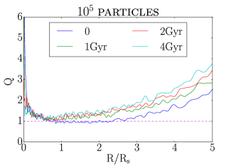
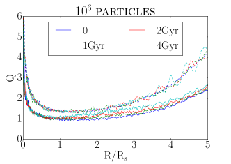
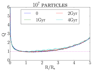
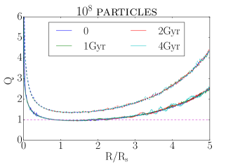
Figure 18: Toomre’s $Q$ parameter as a function of radius. Plots for four identical low-$Q$ discs simulated with different number of particles (from $10^{5}$ to $10^{8}$) are shown with solid lines, while high-$Q$ discs with $10^{6}$ and $10^{8}$ particles are shown with dashed lines in the right-hand panels. Lines of different colour stand for different times, as annotated in legends. In particular, blue lines in each plot denote the $Q$–$r$ relation at the initial time. The swing amplification is strong if $Q$ is close to 1. As spiral structures develop, the ‘temperature’ of the disc raises for low particle numbers, i.e. $10^{5}$ and $10^{6}$, resulting in an increase of $Q$ at later times. This increase of $Q$ coincides with the decrease of spiral strength of corresponding models shown in Fig. 1. For high-$Q$ discs, no prominent spiral structures develop, leading to hardly any changes in $Q$ profile.

The average $Q$ value as a function of radius is shown in Fig. 18. Blue lines denote the $Q$ value in the initial conditions. $Q$ parameter for simulations with low-$Q$ discs is shown with solid curves. For low-$Q$ discs, in the region of $R_{\mathrm{S}}<r<3R_{\mathrm{S}}$, the $Q$ parameter is either less than $1$ or slightly over $1$. Due to the fact that discs are not razor-thin, they are stable to axisymmetric perturbations even when $Q$ is slightly lower than 1, but the swing amplification is still strong. This explains why transient spiral structures are strongest in this region. For simulation with a lower number of particles, $Q$ value grows faster over time. At later times, $Q$ is so high that swing amplification is no longer strong, which leads to the decreasing of spiral strength. In simulations with discs with $Q>1.3$, $Q$ parameter is higher than $1.3$ all through the disc, as shown in the right-hand panels of Fig. 18 with dashed curves. Due to a high $Q$, spiral structures do not grow prominently in the disc.

In conclusion, the growth of self-induced spirals depends on two factors: the initial Poisson noise level and the gravitational stability of the disc. The initial Poisson noise level sets the initial strength of perturbations that are amplified later. The higher number of particles, the longer time it takes to grow perturbations to a prominent level. The stability of the disc decides the actual growth rate of the perturbation. For a highly stable disc, it may take very long time to grow perturbations in a self-induced manner.

Appendix B Discs in Misaligned Triaxial Haloes

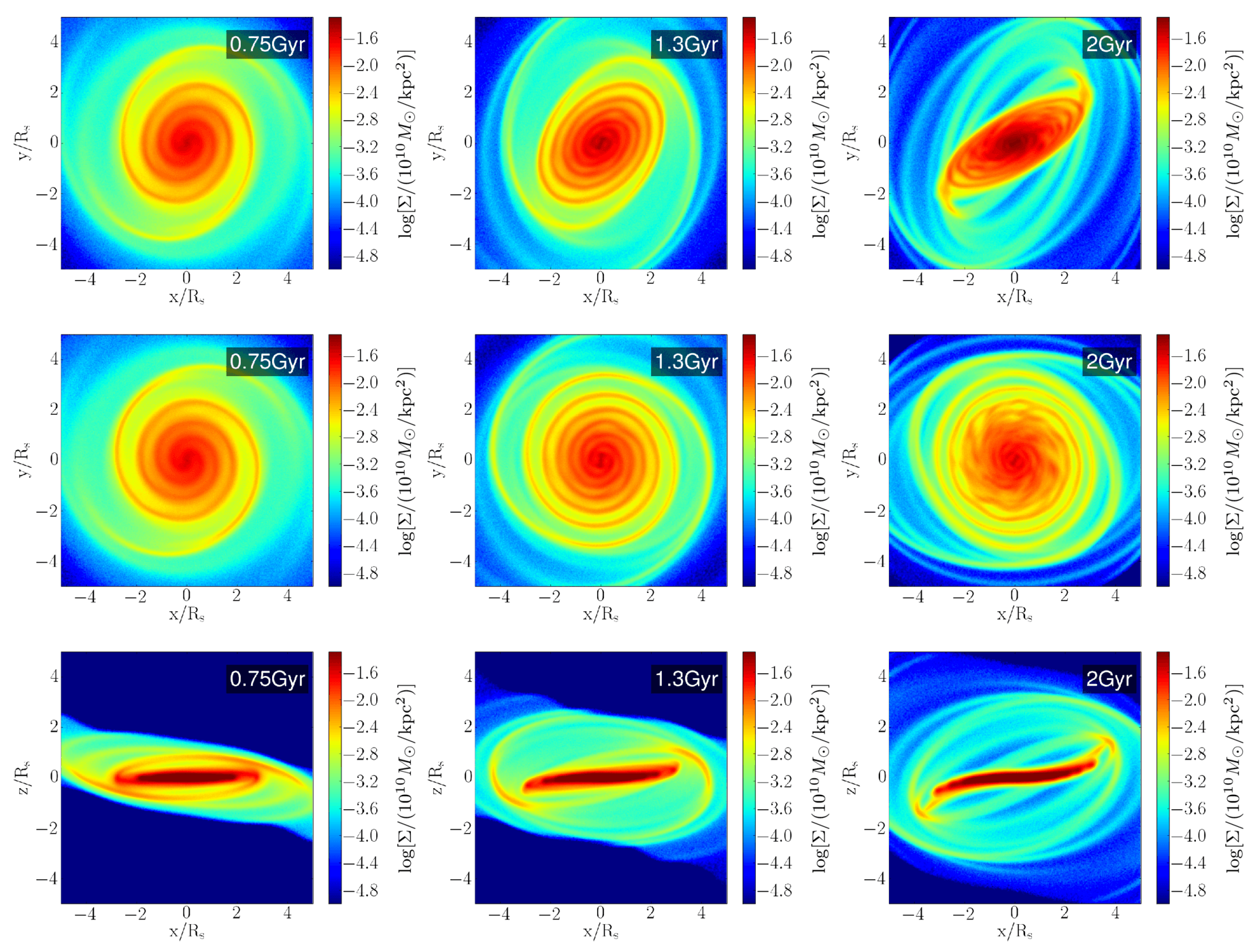
Figure 19: Evolution of a disc in a misaligned triaxial halo. Top: projection of density on the initial plane. Middle: projection of density on the disc plane, whose normal direction is defined by the total angular momentum. Bottom: edge-on column density of the disc. Grand-design two-armed spiral structures still form in this case, while the orientation of the disc is changing as well. It can be also seen from the edge-on plot that warps develop in the disc at later times.

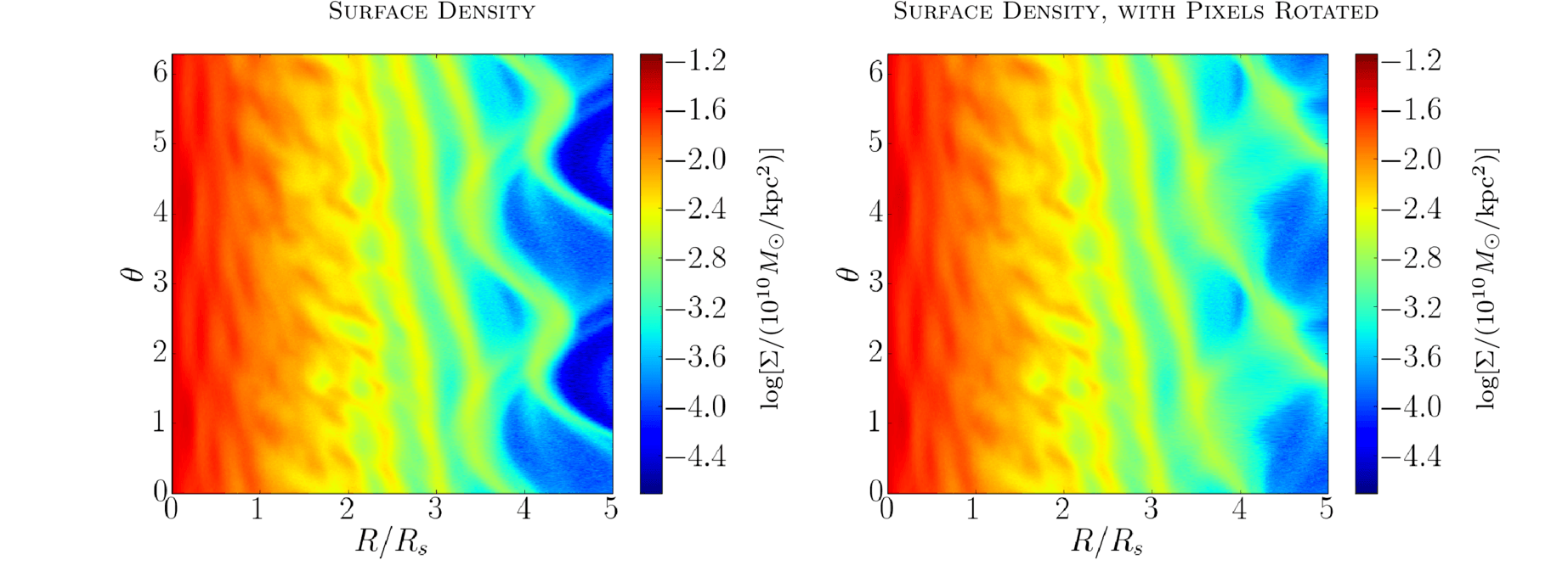
Figure 20: Surface density of a disc in a misaligned triaxial halo at $2\,\mathrm{Gyr}$ in polar coordinates. The outer part of the disc is not in the plane defined by the angular momentum of the disc. The spiral arms are distorted if the density is directly projected on to the disc plane (left). However, if we rotate every pixel on to the disc plane (right), the morphology of the spiral structure becomes similar to the simulations with discs within the $x$–$y$ plane of the haloes.

We now focus on to the influence of triaxial haloes if the disc does not lie in the $x$–$y$ plane of the halo. Even though for isolated systems it has been shown that the inner part of the halo realigns on a dynamical time with the disc (Binney et al., 1998), in cosmological simulations large misalignments are found (e.g. Hahn et al., 2010; Debattista et al., 2013; van de Voort et al., 2015), indicating that discs in misaligned haloes need to be studied. The top row of Fig. 19 shows the projection of the disc on to its initial plane in the simulation with a $T_{\mathrm{O2}}$ halo, i.e. a halo that is more triaxial outside with the disc plane that initially has a 45^∘ angle with respect to the $x$–$y$ plane of the halo, at three different times, $t=0.7,1.3$ and $2\,\mathrm{Gyr}$. At $0.7\,\mathrm{Gyr}$, the overall shape of the projection starts to be compressed. This compression becomes stronger over time. At around $t=2\,\mathrm{Gyr}$, the projection of the disc is strongly compressed in one direction. This compression of the projection on to a fixed plane indicates that the inclination of the disc is changing. In a triaxial halo, the gravity force does not always point directly to the centre. It does not even lie in the disc plane if the disc plane does not coincide with the $x$–$y$, $x$–$z$ or $y$–$z$ plane of the halo. The perpendicular component of the gravity force results in a non-zero torque that is not in the direction of angular momentum, which leads to the change of the disc’s inclination.

We can infer the normal direction of the disc with the direction of the angular momentum vector, as long as the stars stay roughly in a plane. To achieve, this we calculate the total angular momentum

$$\bm{L}=\sum_{i}m\bm{r}_{i}\times\bm{v}_{i}$$ (19)

at each timestep, where $m$ is the mass of a single particle, $\bm{r}_{i}$ and $\bm{v}_{i}$ are the position and velocity vector of the $i$-th star particle.

The middle row of Fig. 19 shows the projection of the disc onto the plane that is perpendicular to the total angular momentum vector. We can see that the morphology of the spiral structures is similar to the disc that is not misaligned with respect to the $x$–$y$ plane of the halo, for example similar to the disc shown in Fig. 12. However, in the outer parts of the disc the shape of the spiral arms is distorted.

We can understand the distortion of the disc by looking at it edge-on. As shown in the bottom row of Fig. 19, the disc develops an integral shape warp at later times, indicating that the disc no longer stays in a plane. Also more and more mass spreads along the $z$ direction. It is also worth noticing that though the warping of the disc shows a trend for the disc to become aligned with the major axis of the halo, which is $45^{\circ}$ from the initial normal direction of the disc, in fact most of the mass of the disc stays in roughly the same initial plane at time $t=2\,\mathrm{Gyr}$.

The warp of the disc before $0.75\,\mathrm{Gyr}$ is very weak. Therefore we can compare the strength of the spiral structures at early times, e.g. $0.5\,\mathrm{Gyr}$, in this simulation with the simulations where the discs lie in the $x$–$y$ plane of the triaxial halo, as shown in the bottom row of Fig. 11 and the right-hand panel of Fig. 10. The strength of the spiral structures in this simulation also matches with the gravitational torque caused by the triaxial halo. In fact, the strength of the torque in this simulation lies between the simulations with $T_{2}$ and $T_{3}$ haloes, as well as the corresponding strength of the spiral structures.

At later times, the outer part of the disc no longer stays in the disc plane. As shown in the middle row of Fig. 19, the outer part of the spiral structures is distorted. We plot the density projection of the disc in polar coordinates, as illustrated in the left-hand panel of Fig. 20. For $R/R_{\mathrm{S}}>3.5$, radius of the spiral structures no longer increases strictly as the angle goes anticlockwise. To investigate if this is due to the warp of the disc, we rotate every pixel in this plot on to the disc plane again while keeping the azimuthal coordinate $\theta$ unchanged, so that the spiral structure all through the disc can be compared on the same plane. This is done by changing the radius $R$ of each pixel to $\sqrt{R^{2}+\overline{z}^{2}}$, where

$$\overline{z}=\frac{1}{\Sigma(R,\theta)}\int_{-\infty}^{\infty}\rho(R,\theta,z)z\mathrm{d}z\,,$$ (20)

is the mean height of the mass at $(R,\theta)$. The result in shown in the right-hand panel of Fig. 20. The radius of the spiral structures increases strictly anticlockwise, as is the case for the spiral structures in all other simulations with discs in the $x$–$y$ plane of the halo. This indicates that the distortion of the outer part of the spiral structures is simply due to the projection.

In conclusion, when the disc is misaligned with the halo, the spiral structures still grow in response to the torque. Their strength corresponds to the strength of the torque, similar to the simulations with discs lying in the halo plane. Even though warps develop at later times, they interfere very little with the spiral structures. The morphology of the spiral structures is unaffected as long as the radii of the spiral structures are calculated with the height from the disc taken into account.

References

- Athanassoula (2012) Athanassoula E., 2012, MNRAS, 426, L46
- Barnes & Efstathiou (1987) Barnes J., Efstathiou G., 1987, ApJ, 319, 575
- Bertin & Lin (1996) Bertin G., Lin C. C., 1996, Spiral Structure in Galaxies a Density Wave Theory. Cambridge, MA MIT Press
- Binney (1978) Binney J., 1978, MNRAS, 183, 779
- Binney et al. (1998) Binney J., Jiang I.-G., Dutta S., 1998, MNRAS, 297, 1237
- Bowden et al. (2013) Bowden A., Evans N., Belokurov V., 2013, MNRAS, 435, 928
- Bryan et al. (2013) Bryan S. E., Kay S. T., Duffy A. R., Schaye J., Dalla Vecchia C., Booth C. M., 2013, MNRAS, 429, 3316
- Debattista et al. (2008) Debattista V. P., Moore B., Quinn T., Kazantzidis S., Maas R., Mayer L., Read J., Stadel J., 2008, ApJ, 681, 1076
- Debattista et al. (2013) Debattista V. P., Roškar R., Valluri M., Quinn T., Moore B., Wadsley J., 2013, MNRAS, 434, 2971
- DeBuhr et al. (2012) DeBuhr J., Ma C.-P., White S. D., 2012, MNRAS, 426, 983
- Dobbs & Baba (2014) Dobbs C., Baba J., 2014, Publ. Astron. Soc. Australia, 31, 35
- Dobbs & Bonnell (2006) Dobbs C. L., Bonnell I. A., 2006, MNRAS, 367, 873
- Dobbs & Bonnell (2007) Dobbs C. L., Bonnell I. A., 2007, MNRAS, 376, 1747
- D’Onghia et al. (2010) D’Onghia E., Springel V., Hernquist L., Keres D., 2010, ApJ, 709, 1138
- D’Onghia et al. (2013) D’Onghia E., Vogelsberger M., Hernquist L., 2013, ApJ, 766, 34
- Dubinski (1994) Dubinski J., 1994, ApJ, 431, 617
- Dubinski & Chakrabarty (2009) Dubinski J., Chakrabarty D., 2009, ApJ, 703, 2068
- Fouvry & Pichon (2015) Fouvry J.-B., Pichon C., 2015, MNRAS, 449, 1982
- Fouvry et al. (2015) Fouvry J. B., Pichon C., Magorrian J., Chavanis P. H., 2015, A&A, 584, A129
- Franx & de Zeeuw (1992) Franx M., de Zeeuw T., 1992, ApJ, 392, L47
- Frenk et al. (1988) Frenk C. S., White S. D., Davis M., Efstathiou G., 1988, ApJ, 327, 507
- Fujii et al. (2011) Fujii M. S., Baba J., Saitoh T. R., Makino J., Kokubo E., Wada K., 2011, ApJ, 730, 109
- Gittins & Clarke (2004) Gittins D. M., Clarke C., 2004, MNRAS, 349, 909
- Grand et al. (2012a) Grand R. J. J., Kawata D., Cropper M., 2012a, MNRAS, 426, 167
- Grand et al. (2012b) Grand R. J. J., Kawata D., Cropper M., 2012b, MNRAS, 421, 1529
- Hahn et al. (2010) Hahn O., Teyssier R., Carollo C. M., 2010, MNRAS, 405, 274
- Hernquist (1990) Hernquist L., 1990, ApJ, 356, 359
- Jing et al. (1995) Jing Y., Mo H., Börner G., Fang L., 1995, MNRAS, 276, 417
- Jing & Suto (2002) Jing Y., Suto Y., 2002, ApJ, 574, 538
- Julian & Toomre (1966) Julian W. H., Toomre A., 1966, ApJ, 146, 810
- Kalnajs (1973) Kalnajs A., 1973, in Proceedings of the Astronomical Society of Australia Vol. 2, Spiral structure viewed as a density wave. p. 174
- Khoperskov et al. (2013) Khoperskov A. V., Khoperskov S. A., Zasov A. V., Bizyaev D. V., Khrapov S. S., 2013, MNRAS, 431, 1230
- Khoperskov & Bertin (2015) Khoperskov S. A., Bertin G., 2015, MNRAS, 451, 2889
- Lin & Shu (1964) Lin C., Shu F. H., 1964, ApJ, 140, 646
- Lindblad (1956) Lindblad B., 1956, Stockholms Observatoriums Annaler, 19, 7
- Lindblad (1963) Lindblad B., 1963, Stockholms Observatoriums Annaler, 22, 5
- Purcell et al. (2011) Purcell C. W., Bullock J. S., Tollerud E. J., Rocha M., Chakrabarti S., 2011, Nature, 477, 301
- Romeo (1992) Romeo A. B., 1992, MNRAS, 256, 307
- Salo et al. (2010) Salo H., Laurikainen E., Buta R., Knapen J. H., 2010, ApJ, 715, L56
- Sellwood (2012) Sellwood J. A., 2012, ApJ, 751, 44
- Sellwood & Carlberg (2014) Sellwood J. A., Carlberg R. G., 2014, ApJ, 785, 137
- Springel (2005) Springel V., 2005, MNRAS, 364, 1105
- Springel et al. (2005) Springel V., Di Matteo T., Hernquist L., 2005, MNRAS, 361, 776
- Springel et al. (2008) Springel V., Wang J., Vogelsberger M., Ludlow A., Jenkins A., Helmi A., Navarro J. F., Frenk C. S., White S. D., 2008, MNRAS, 391, 1685
- Thomas et al. (1998) Thomas P. A., Colberg J. M., Couchman H. M., Efstathiou G. P., Frenk C. S., Jenkins A. R., Nelson A. H., Hutchings R. M., Peacock J. A., Pearce F. R., et al., 1998, MNRAS, 296, 1061
- Toomre (1964) Toomre 1964, ApJ, 139, 1217
- Toomre (1981) Toomre 1981, in Structure and Evolution of Normal Galaxies Vol. 1, What amplifies the spirals. pp 111–136
- van de Voort et al. (2015) van de Voort F., Davis T. A., Kereš D., Quataert E., Faucher-Giguère C.-A., Hopkins P. F., 2015, MNRAS, 451, 3269
- Vandervoort (1970) Vandervoort P. O., 1970, ApJ, 161, 87
- Vera-Ciro et al. (2011) Vera-Ciro C. A., Sales L. V., Helmi A., Frenk C. S., Navarro J. F., Springel V., Vogelsberger M., White S. D. M., 2011, MNRAS, 416, 1377
- Warren et al. (1992) Warren M. S., Quinn P. J., Salmon J. K., Zurek W. H., 1992, ApJ, 399, 405
- Yoshida et al. (2000) Yoshida N., Springel V., White S. D., Tormen G., 2000, ApJLetters, 544, L87
- Zemp et al. (2012) Zemp M., Gnedin O. Y., Gnedin N. Y., Kravtsov A. V., 2012, ApJ, 748, 54
- Zhu et al. (2016) Zhu Q., Marinacci F., Maji M., Li Y., Springel V., Hernquist L., 2016, MNRAS, 458, 1559