The Epsilon Eridani System Resolved by Millimeter Interferometry

Abstract

We present observations of $\epsilon$ Eridani from the Submillimeter Array (SMA) at 1.3 millimeters and from the Australia Telescope Compact Array (ATCA) at 7 millimeters that reach an angular resolution of $\sim 4\arcsec$ (13 AU). These first millimeter interferometer observations of $\epsilon$ Eridani, which hosts the closest debris disk to the Sun, reveal two distinct emission components: (1) the well-known outer dust belt, which, although patchy, is clearly resolved in the radial direction, and (2) an unresolved source coincident with the position of the star. We use direct model-fitting of the millimeter visibilities to constrain the basic properties of these two components. A simple Gaussian shape for the outer belt fit to the SMA data results in a radial location of $64.4^{+2.4}_{-3.0}$ AU and FWHM of $20.2^{+6.0}_{-8.2}$ AU (fractional width $\Delta R/R=0.3$). Similar results are obtained taking a power law radial emission profile for the belt, though the power law index cannot be usefully constrained. Within the noise obtained (0.2 mJy beam^-1), these data are consistent with an axisymmetric belt model and show no significant azimuthal structure that might be introduced by unseen planets in the system. These data also limit any stellocentric offset of the belt to $<9$ AU, which disfavors the presence of giant planets on highly eccentric ($>0.1$) and wide (10’s of AU) orbits. The flux density of the unresolved central component exceeds predictions for the stellar photosphere at these long wavelengths, by a marginally significant amount at 1.3 millimeters but by a factor of a few at 7 millimeters (with brightness temperature $13000\pm 1600$ K for a source size of the optical stellar radius). We attribute this excess emission to ionized plasma from a stellar corona or chromosphere.

1 Introduction

Debris disks, composed of planetesimals remaining after planet formation and circumstellar disk dispersion, represent the end-stage of protoplanetary disk evolution (see reviews by Backman & Paresce, 1993; Wyatt, 2008; Matthews et al., 2014). While these remnant planetesimals cannot be observed directly, they are ground down through ongoing collisions into smaller and smaller dust grains that scatter starlight and produce detectable thermal emission. Observations of this dusty debris at millimeter wavelengths are especially critical to our understanding of the most readily accessible systems. The large grains that dominate emission at these long wavelengths do not travel far from their origin and therefore reliably trace the underlying planetesimals distribution, unlike the small grains that are rapidly removed by stellar radiation and winds (Wyatt, 2006). Since planets, if present, will inevitably perturb the dust-producing planetesimals, the millimeter emission morphology encodes information on the architecture and dynamical evolution of these systems. For example, the outward migration of a planet can confine planetesimals in a belt between its resonances (Hahn & Malhotra, 2005), or trap planetesimals into mean motion resonances outside its orbit (Kuchner & Holman, 2003; Wyatt, 2003; Deller & Maddison, 2005). A planet can also sculpt out sharp edges in a belt (Quillen, 2006; Chiang et al., 2009), or force planetesimals onto eccentric or inclined orbits (Wyatt et al., 1999).

At a distance of only 3.22 pc (van Leeuwen, 2007), the $400-800$ Myr-old (Mamajek & Hillenbrand, 2008) main-sequence K2 star $\epsilon$ Eridani hosts the closest debris disk to the Sun, originally identified through the detection of far-infrared emission by IRAS (Aumann, 1985). Pioneering observations with JCMT/SCUBA resolved a nearly face-on belt of emission at 850 $\mu$m, peaking at 60 AU ($18\arcsec$) radius, with several brightness enhancements or clumps (Greaves et al., 1998). Analysis by Greaves et al. (2005) of JCMT images spanning 5 years offered tentative evidence that some of these clumps are stationary, and so likely background galaxies, while others appear to be co-moving with the star, and so are likely associated with the disk. Subsequent single-dish observations from 250 to 1200 $\mu$m have confirmed the basic belt morphology, but not all of the low significance asymmetries (Schütz et al., 2004; Backman et al., 2009; Greaves et al., 2014; Lestrade & Thilliez, 2015). A warmer dust component, reaching to several AU from the star, can be explained in modeling the spectral energy distribution by an additional dust belt (Backman et al., 2009; Greaves et al., 2014), or by inward transport from the outer belt (Reidemeister et al., 2011). In addition, precision radial velocity observations suggest the presence of a Jupiter-mass planet with semi-major axis of 3.4 AU ($1^{\prime\prime}$) (Hatzes et al., 2000), although the reality of this planet signal remains controversial (Anglada-Escudé & Butler, 2012). Because $\epsilon$ Eridani is so nearby, it is a key template for understanding debris disk phenomena around Sun-like stars, and detailed study of its debris disk provides essential context for the interpretation of more distant, less accessible systems.

We present observations of $\epsilon$ Eridani at 1.3 mm and at 7 mm, using the Submillimeter Array (SMA) and the Australia Telescope Compact Array (ATCA), respectively, using the most compact, lowest angular resolution ($4^{\prime\prime}-10^{\prime\prime}$) configurations of these telescopes. While even higher resolution may be desirable, these interferometric observations are conservatively tuned to provide a first look at structures below the resolution of previous single dish observations. For these arrays at these wavelengths, the primary beam field of view encompasses the entire emission region from the outer debris belt, enabling efficient observations of the full disk with a single pointing. Section 2 describes these observations of the $\epsilon$ Eridani system. Section 3 describes the modeling procedure and the results. Section 4 discusses the implications of the model fits for the outer dust belt properties, azimuthal asymmetries, and the nature of an inner component of excess millimeter emission.

2 Observations

2.1 Submillimeter Array

We observed $\epsilon$ Eridani in July, August and November 2014 with the SMA (Ho et al., 2004) on Mauna Kea, Hawaii at a wavelength of 1.3 mm in the subcompact configuration. Table 1 summarizes the essentials of these observations, including the dates, baseline lengths, and atmospheric opacity. Six tracks were obtained, all with 7 operational antennas in the array. The weather conditions were very good for observations at this wavelength (225 GHz opacities from 0.07 to 0.12). The total bandwidth available was 8 GHz consisting of two sidebands of 4 GHz width spanning $\pm 4$ to 8 GHz from the local oscillator (LO) frequency of 225.5 GHz ($217.5-221.5$ GHz and $229.5-233.5$ GHz). The phase center was located at $\alpha=03^{\text{h}}32^{\text{m}}54\fs 9024$, $\delta=-09\arcdeg 27\arcmin 29\farcs 4486$ (J2000), corresponding to the position of the star corrected for its proper motion of (-975.17,19.49) mas yr^-1 (van Leeuwen, 2007) as of July 1, 2014 . At the LO frequency, the field of view is $\sim 52\arcsec$, set by the primary beam size of the 6-m diameter array antennas.

The data from each track were calibrated independently using the IDL-based MIR software package. Time-dependent complex gains were determined from observations of two nearby quasars, J0339-017 ($7\fdg 9$ away) and J0423-013 ($14\fdg 9$ away), interleaved with observations of $\epsilon$ Eridani in a 16 minute cycle. The passband shape was calibrated using available bright sources, mainly 3C84 or 3C454.3. Observations of Uranus or Callisto during each track were used to derive the absolute flux scale with an estimated accuracy of $\sim 10\%$. Imaging and deconvolution were performed with the clean task in the CASA software package. A variety of visibility weighting schemes were used to explore compromises in imaging between higher angular resolution and better surface brightness sensitivity. With natural weighting, the beam size is $6\farcs 0\times 5\farcs 5$ ($19\times 18$ AU) and the rms noise level is 0.17 mJy beam^-1. The longest baselines in the dataset probe size scales of $\sim 4^{\prime\prime}$ (13 AU).

2.2 Australia Telescope Compact Array

We observed $\epsilon$ Eridani in late June and early August 2014 with the ATCA, located near Narrabri, NSW, at a wavelength of 7 mm using the compact H75 and H168 configurations of the array. Table 2 summarizes the essentials of these observations. Four tracks were obtained in each of the two antenna configurations, all with 6 operational antennas. The winter weather provided good atmospheric phase stability for this ATCA high frequency band (rms path typically $<150$ microns from the seeing monitor), especially for the short baselines of interest, except for the last track in the H168 configuration (2014 July 28), which proved to be unusable due to high winds and relatively poor seeing. Data from the stationary sixth antenna of the array, located $\sim 6$ km from the others, was discarded, given the large gap from the rest of the antennas and less stable phase on the much longer baselines. The bandwidth provided by the Compact Array Broadband Backend was 8 GHz, with 2 GHz wide bands centered at 43 GHz and at 45 GHz, in two polarizations (Wilson et al., 2011). The phase center was identical to the contemporaneous SMA observations. The field of view is $\sim 70\arcsec$, set by the primary beam size of the 22-m diameter array antennas.

The data from the seven usable tracks were calibrated independently using the miriad software package. Time-dependent complex gains were determined using the nearby quasar 0336-019 ($7\fdg 8$ away), interleaved with observations of $\epsilon$ Eridani in a 12 minute cycle. The passband shape was calibrated using the available bright sources 1921-293 or 0537-441. Observations of 1934-638 and Uranus during each track were used to derive the absolute flux scale. Comparison of the derived fluxes for 0336-019 for each of the seven nights shows a maximum difference of 6%, and we conservatively estimate the flux scale accuracy is better than $10\%$. Imaging and deconvolution were performed with the standard routines invert, clean, and restor in the miriad software package.

3 Results and Analysis

3.1 Continuum Emission

Figure 1 shows an SMA 1.3 mm image and ATCA 7 mm image of $\epsilon$ Eridani, together with the Herschel/SPIRE 250 $\mu$m image extracted from the Herschel Science Archive for reference (Greaves et al., 2014). For the 1.3 mm image, the synthesized beam size, obtained with natural weighting and a modest taper to improve surface brightness sensitivity is $9\farcs 2\times 8\farcs 7$ ($30\times 28$ AU), position angle $68\arcdeg$. The rms noise is 0.20 mJy beam^-1. This image reveals emission from a compact central source at the stellar position ($\sim 7\sigma$) together with patchy emission from the nearly face-on belt of cold dust located $\sim 18^{\prime\prime}$ from the star. For the 7 mm image, the synthesized beam size obtained with natural weighting is $9\farcs 2\times 7\farcs 0$ ($30\times 23$ AU), position angle $83\arcdeg$. The rms noise is $7$ $\mu$Jy beam^-1. A central peak is clearly detected ($\sim 10\sigma$). Unlike the 1.3 mm image, the 7 mm image shows little sign of emission from the outer dust belt. In both images, the position of the central peak is consistent with the predicted stellar position, within the uncertainty dictated by the synthesized beam size, $\theta$, and the signal-to-noise ratio, $SNR$ of $\sim 0.5\theta/{SNR}\approx 0\farcs 6$ (see Reid et al., 1988).

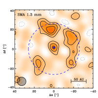
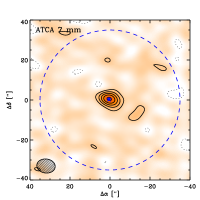
Figure 1: (left) Herschel/SPIRE 250 $\mu$m image of $\epsilon$ Eridani, from the Herschel Science Archive (see also Greaves et al., 2014). The ellipse in the lower left indicates the $\sim 19\arcsec$ beam size. (center) SMA image of the 1.3 millimeter continuum emission from $\epsilon$ Eridani. The contour levels are in steps of $2\times 0.2$ mJy, the rms noise level. The ellipse in the lower left corner indicates the $9\farcs 2\times 8\farcs 7$ (FWHM) synthesized beam size. The dashed blue circle indicates the $\sim 52\arcsec$ SMA primary beam (FWHM) at the LO frequency (225.5 GHz). (right) ATCA image of the 7 millimeter continuum emission from $\epsilon$ Eridani. The contour levels are in steps of $2\times 7$ $\mu$Jy, the rms noise level. The ellipse in the lower left corner indicates the $9\farcs 2\times 7\farcs 0$ (FWHM) synthesized beam size. The dashed blue circle indicates the $\sim 70\arcsec$ ATCA primary beam (FWHM) at 44 GHz. In all three panels, the star symbol marks the position of the stellar photosphere, corrected for proper motion. For the center and right panels, the stellar position is: $\alpha=03^{\text{h}}32^{\text{m}}54\fs 9024$, $\delta=-09\arcdeg 27\arcmin 29\farcs 4486$ (J2000).

3.2 Emission Modeling Procedure

To characterize the 1.3 mm emission from $\epsilon$ Eridani, we used the procedure described by MacGregor et al. (2013, 2015) that employs a Markov Chain Monte Carlo (MCMC) method to fit simple parametric models to the observed visibilities. We fit the visibility data directly both to avoid the non-linear effects of deconvolution and to take advantage of the full range of spatial frequencies in the observations that are not necessarily represented well in the images. We assume that the emission arises from a geometrically thin, axisymmetric belt, where we consider two different parametric shapes for the surface brightness profile, $I_{\nu}(r)$: (1) an annulus with $R_{\text{in}}<r<R_{\text{out}}$ and power law slope, $I_{\nu}(r)\propto r^{x}$, and (2) a Gaussian, $I_{\nu}(r)\propto\text{exp}[-((r-R_{\text{cen}})/\sqrt{2}\sigma)^{2}]$, where $R_{\text{cen}}$ is the position of the belt, $\sigma$ is the width, and the FWHM $=\Delta R=2\sqrt{2\text{ln}(2)}\times\sigma$. The limited signal-to-noise of the dataset precludes exploring more complicated, but physically plausible, surface brightness shapes, such as multiple rings or a broken power law. The belt emission normalization is defined by a total flux density, $F_{\text{belt}}=\int I_{\nu}d\Omega$, and the belt center is given by offsets relative to the pointing center $\{\Delta\alpha,\Delta\delta\}$. The central peak coincident with the stellar position is described by a point source with total flux, $F_{\text{cen}}$, and the offsets of this point source relative to the belt center are given by two additional parameters $\{\Delta\alpha_{\text{star}},\Delta\delta_{\text{star}}\}$. The previous imaging observations show that the belt is viewed close to face-on ($i=30\arcdeg$, Greaves et al., 2014). We fit the SMA data directly for an inclination angle, $i$, and also an orientation on the sky described by a position angle, $PA$, east of north.

The $\epsilon$ Eridani disk spans a large angle on the sky, approaching (or possibly exceeding) the half power field of view of the SMA. As a result, the primary beam response has the potential to affect the properties derived for the outer regions of the millimeter emission belt. To account for this in the analysis, we multiply each belt model by an accurate, frequency-dependent beam model, normalized to unity at the beam center. Appendix A provides a detailed discussion of the SMA primary beam shape. For ATCA, with its larger field of view at the observed wavelength, the effects of the primary beam shape are much less important, and a simple Gaussian provides an adequate description.

For each set of model parameters, we use the miriad uvmodel task to compute two synthetic visibility sets sampled at the same spatial frequencies as our SMA observations, corresponding to the two spectrally averaged sidebands (218.9 and 230.9 GHz). The fit quality is characterized by a likelihood metric, $\mathcal{L}$, determined from the $\chi^{2}$ values computed using the real and imaginary components at all spatial frequencies (ln$\mathcal{L}=-\chi^{2}/2$). This modeling scheme is implemented using the affine-invariant ensemble MCMC sampler proposed by Goodman & Weare (2010) and realized in Python by Foreman-Mackey et al. (2013). A MCMC approach allows us to more effectively characterize the multidimensional parameter space of this model and to determine the posterior probability distribution functions for each parameter. We assumed uniform priors for all parameters, with reasonable bounds imposed to ensure that the model was well-defined: $F_{\text{belt}}\geq 0$ and $0\leq R_{\text{in}}<R_{\text{out}}$. In addition, we constrained the four offset parameters $\{\Delta\alpha,\Delta\delta,\Delta\alpha_{\text{star}},\Delta\delta_{\text{star}}\}$ that describe the belt center and stellar position to be within $5\arcsec$ of the offsets predicted from the stellar proper motion; this constraint very generously accommodates the uncertainties in the proper motion and the absolute astrometry of the observations.

For the ATCA 7 mm observations, where the $\epsilon$ Eridani emission belt is not visible in the image, we simplified the model substantially. We fix all of the model parameters to the best-fit values from the analysis of the SMA data, except the total belt flux ($F_{\text{belt}}$), the total flux for the central peak ($F_{\text{cen}}$), and two position offsets $\{\Delta\alpha,\Delta\delta\}$. In essence, we fix the shape of the emission structure to that found from analysis of the SMA data, and we determine the 7 mm fluxes for the central component and for the belt component, allowing for the possibility of a small positional shift between the SMA and ATCA datasets. We do not constrain $F_{\text{belt}}$ to be positive as for the SMA observations

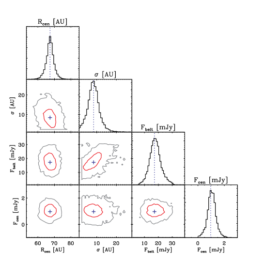
Figure 2: A sample of the output from a run of $\sim 10^{4}$ MCMC trials for the 4 best-fit Gaussian belt geometry parameters ($R_{\text{cen}}$, $\sigma$, $F_{\text{belt}}$, and $F_{\text{cen}}$). The diagonal panels show the 1D histogram for each parameter marginalized over all other parameters considered in the model. For each parameter, the peak of each histogram is taken to be the best-fit value. The remaining panels show contour plots of the $1\sigma$ (red) and $2\sigma$ (gray) regions for each pair of parameters, with the blue crosses marking the best-fit values.

3.3 Results of Model Fits

Table 3 lists the resulting best-fit parameter values and their $68\%$ uncertainties determined from the marginalized posterior probability distributions for both the power law and Gaussian belt models fit to the SMA 1.3 mm data. Figure 2 shows a sample of the output for the main Gaussian belt parameters, including the marginalized posterior probability distributions. The $1\sigma$ and $2\sigma$ regions are determined by assuming normally distributed errors, where the probability that a measurement has a distance less than $a$ from the mean value is given by $\text{erf}\left(\frac{a}{\sigma\sqrt{2}}\right)$. Both of these functional forms provide good fits to the observed visibilities, with reduced $\chi^{2}$ values of about $1.4$ (59,924 independent data points, 11 and 10 free parameters for the power law and Gaussian models, respectively) for each. Figure 3 shows the best-fit models of the 1.3 mm data in the image plane, at the full resolution of the models, and imaged like the SMA data, both without noise and with the noise level obtained by the observations, which results in patchy outer belt emission very similar to the SMA image in Figure 1. The imaged residuals are also shown in Figure 3, and these are mostly noise (see Section 4.1.5 for further discussion of the residuals from these axisymmetric models).

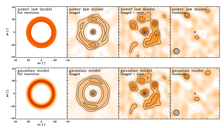
Figure 3: Images of the best-fit models to the SMA 1.3 mm emission. (Upper): (left) the best-fit power law disk model at full resolution, pixel scale $\sim 0\farcs 2$ (0.8) AU, and (center, left) image of the best-fit power law disk model with no noise, (center, right) the best-fit power law disk model with simulated noise, and (right) the imaged residuals from the power law disk model, made using the same imaging parameters as in Figure 1. (Lower): (left) the best-fit Gaussian disk model at full resolution, and (center, left) image of the best-fit Gaussian disk model, (center, right) image with simulated noise of the best-fit Gaussian disk model, and (right) the imaged residuals from the Gaussian disk model, again made using the same imaging parameters as in Figure 1. The contour levels are at 0.4 mJy beam^-1 ($2\sigma$) intervals in all panels. The ellipse in the lower left corner of the residual images indicates the $9\farcs 2\times 7\farcs 0$ (FWHM) synthesized beam size.

A useful way of visualizing the interferometric data and model fits is through the deprojected visibility function, which takes advantage of (near) axisymmetry to reduce the dimensionality (Lay et al., 1997). In particular, the real part of the complex visibilities are averaged in concentric annuli of deprojected $(u,v)$ distance, $\mathcal{R}_{uv}$, from the center of the emission structure. Figure 4 shows this view of the SMA 1.3 mm data together with the best-fit power law and Gaussian belt models. The result is a function with a zero-crossing null and several subsequent oscillations. Although these SMA observations are missing the short $(u,v)$ spacings needed to sample the peak of the visibility function, the overall shape matches nicely that expected for a narrow annulus of emission, plus a small and constant positive offset contribution from an unresolved central source. Figure 4 also shows the single dish flux measurements at the zero-spacing of the deprojected visibility function (with small offsets from zero for clarity). It is remarkable that the simple axisymmetric belt models of the SMA data appear to provide a very good estimate of the total flux, despite the lack of shorter baseline data. This consistency provides indirect support for the basic model of the emission distribution.

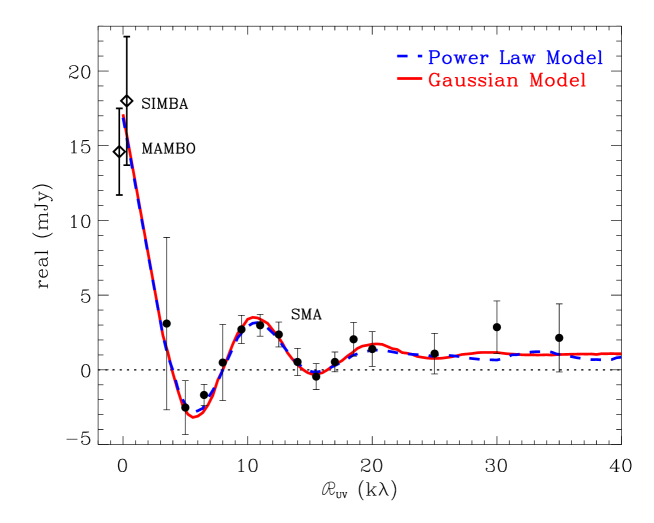
Figure 4: The real part of the SMA 1.3 mm visibilities averaged in bins of deprojected (u,v) distance from the disk center, compared to the best-fit power law (dashed blue) and Gaussian (solid red) disk models plus a central point-source. The single dish MAMBO-2/IRAM (Lestrade & Thilliez, 2015) and SIMBA fluxes (Schütz et al., 2004) extrapolated from 1.2 mm to 1.3 mm are plotted at $\mathcal{R}_{uv}=0$ k$\lambda$ (slightly offset from zero, for viewing clarity).

Table 4 lists the best-fit parameter values from the modeling and their $68\%$ uncertainties for the 7 mm data. This model again provides a good fit to the data, with reduced $\chi^{2}=1.32$ (151,976 independent data points, 4 free parameters). We note that the best-fit belt flux at 7 mm is positive, albeit with low statistical significance; this positive value suggests the presence of emission below the detection threshold in individual beams in the image. The position offsets between the ATCA and SMA data are small, consistent with zero.

4 Discussion

We have performed interferometric observations of the $\epsilon$ Eridani system at 1.3 mm and 7 mm with the SMA and the ATCA, respectively, with baselines that sample to $\sim 4^{\prime\prime}$ (13 AU) resolution. The 1.3 mm image reveals emission from a resolved outer dust belt located $\sim 18\arcsec$ (60 AU) from the star, and a compact source coincident with the stellar position. The 7 mm image shows only a central peak, detected with greater significance than in the 1.3 mm image. We modeled the visibility data assuming two emission components, an outer belt with a power law or Gaussian radial surface brightness profile, and a central point source. Both functional forms provide good fits to the 1.3 mm data, and we used the best-fit emission shape parameters to obtain constraints on the component flux densities from the 7 mm data. We now use the new information about these emission components to discuss implications for the debris disk and to compare to claims derived from previous millimeter and submillimeter observations with lower angular resolution.

4.1 Outer Belt

Several basic properties of the outer emission belt are strongly constrained by the SMA 1.3 mm observations, including its flux, radial location and width, viewing geometry, and departures from axisymmetry. These new constraints bear on the possible presence of unseen planets in the system.

4.1.1 Belt Flux

The total flux density of the best-fit power law and Gaussian models, is constrained to be $F_{\text{belt}}=16.9^{+3.9}_{-5.6}$ mJy and $17.2^{+5.1}_{-4.5}$ mJy, respectively. These values are consistent with each other, within the uncertainties. They are also consistent with previous single-dish mapping measurements in this atmospheric window, accounting for minor differences in effective wavelength due to the broadband nature of bolometer detectors. Lestrade & Thilliez (2015) obtained a total flux density of $17.3\pm 3.5$ mJy using MAMBO-2 on the IRAM 30-m telescope and Schütz et al. (2004) measured a total flux density of $21.4\pm 5.1$ mJy using SIMBA with the SEST 15-m telescope. If we extrapolate these measurements using the spectral index of $\sim 2.14$ derived for $\epsilon$ Eridani at submillimeter wavelengths (Gáspár et al., 2012), we find close agreement with the values obtained from the SMA analysis. In particular, extrapolating the IRAM/MAMBO-2 observation to 1.3 mm gives $14.6\pm 2.9$ mJy, while the older SIMBA observation gives $18.0\pm 4.3$ mJy (see Figure 4).

4.1.2 Belt Location and Width

For the best-fit power law model, the outer radius of the millimeter emission belt is determined to be $R_{\text{out}}=80.2^{+3.0}_{-7.1}$ AU. Previous imaging studies of $\epsilon$ Eridani provide estimates of the outer radius between $70-90$ AU, in good agreement with this determination (Greaves et al., 1998, 2005, 2014; Backman et al., 2009). Additionally, we constrain the inner radius of the power law model, $R_{\text{in}}=53.4^{+6.1}_{-5.0}$ AU. This value agrees most closely with analysis of 160 $\mu$m Herschel observations by Greaves et al. (2014), which also suggest an inner radius of the outer belt of $\sim 54$ AU. Other single-dish observations indicated that the belt extends further inward towards the star, $R_{\text{in}}=35-40$ AU (Greaves et al., 1998, 2005; Backman et al., 2009). The model fits to the SMA 1.3 mm data do not support such a wide belt with an inner radius so close to the star.

The best-fit Gaussian model is characterized by a radial location, $R_{\text{cen}}=64.4^{+2.4}_{-3.0}$ AU, and a width, $\sigma=8.55^{+2.54}_{-3.46}$ AU, or FWHM $=\Delta R=2\sqrt{2\text{ln}(2)}\times\sigma=20.2^{+6.0}_{-8.2}$ AU. These parameters are most directly comparable to the belt parameters derived by Lestrade & Thilliez (2015) using IRAM/MAMBO-2 observations at 1.2 mm with a telescope FWHM beam size of $10\farcs 7$; they fit a Gaussian shape to the disk emission radial profile and obtain a central radius $R_{\text{cen}}=57\pm 1.3$ AU, FWHM $=12\arcsec\pm 1\arcsec$, and infer $8\leq\Delta R\leq 22$ AU. This central radius is slightly smaller than that derived from the SMA data, but plausibly consistent within the mutual uncertainties. Since the lower limit on the width is narrower than implied by the fit to the SMA data at the 68% confidence interval, we examine this potential discrepancy more closely.

The effect of changing the belt location ($R_{\text{cen}}$) and width ($\sigma$) is dramatic on the null locations in the deprojected visibility function. We expressed our Gaussian model using a surface brightness profile of the form $I_{\nu}(r)=A\times\text{exp}[-((r-R_{\text{cen}})/\sqrt{2}\sigma)^{2}]$. The Fourier transform of a radially symmetric function like this can be expressed by a Hankel transform:

$$F(\rho)=2\pi A\int_{0}^{\infty}I_{\nu}(r)J_{0}(\rho r)rdr,$$ (1)

where, $\rho=2\pi\sqrt{u^{2}+v^{2}}=2\pi\mathcal{R}_{uv}$. For a Gaussian ring, there is an exact solution to this integral involving an infinite series of hypergeometric functions that can be evaluated numerically to find the exact locations of the visibility nulls. Fortunately, there is also an approximate solution to the Hankel transform using a generalized shift operator (described in Baddour, 2009) that yields the values of the null locations to within 1% of the exact solution,

$$F(\rho)=2\pi A\sigma^{2}\times\text{exp}[-(\rho\sqrt{2}\sigma)^{2}/4]\times J_{0}(\rho R_{\text{cen}}),$$ (2)

From this simple expression, we can see immediately that for a fixed belt width, decreasing the belt radius (inward towards the star) moves the zero-crossing null locations towards larger $\mathcal{R}_{uv}$. For a fixed belt location, decreasing the belt width moves the zero-crossing null locations towards slightly smaller $\mathcal{R}_{uv}$ (and increases the amplitude of subsequent oscillations). The best-fit Gaussian model to the SMA data, $R_{\text{cen}}=64$ AU, $\sigma=8.6$ AU yields nulls at $\mathcal{R}_{uv}\approx 4$, 8, and 14 k$\lambda$. By comparison, a Gaussian model with $R_{\text{cen}}=57$ AU and $\Delta R=8$ AU ($\sigma\sim 4$ AU), at the lower limit of width suggested by Lestrade & Thilliez (2015), results in nulls at $\mathcal{R}_{uv}\approx 5$, 9, and 16 k$\lambda$, which are significantly offset from the data. The differences between these fit results may stem from the oversimplified assumption of a strict Gaussian shape for the emission, perhaps exacerbated by deconvolution of the synthesized beam resulting from the shift-and-add procedure used to restore the MAMBO map from the chopped observations of the $\epsilon$ Eridani field.

The presence of planets can affect the widths of planetesimal belts, through dynamical interactions. Given the best-fit Gaussian belt parameters, we can constrain the fractional belt width of the $\epsilon$ Eridani debris disk to $\Delta R/R=0.31^{+0.09}_{-0.13}$. This fractional width lies within the range of $0.1\leq\Delta R/R\leq 0.4$ obtained by Lestrade & Thilliez (2015). For comparison, the classical Kuiper Belt in our Solar System appears radially confined between 40 and 48 AU ($\Delta R/R\sim 0.18$), filling the region between the 3:2 and 2:1 resonances with Neptune, likely the result of its outward migration (Hahn & Malhotra, 2005). A narrow ring of millimeter emission in the Fomalhaut debris disk (FWHM $\sim 16$ AU and $\Delta R/R\sim 0.1$) has been attributed to confinement by shepherding planets orbiting inside and outside the ring (Boley et al., 2012). The best-fit value of the fractional width of the $\epsilon$ Eridani belt is wider than the Fomalhaut belt and the classical Kuiper Belt, but not as wide as the belt surrounding the Sun-like star HD 107146, which also shows hints of a more complex radial structure (Ricci et al., 2015).

The SMA 1.3 mm data do not place any strong constraints on the sharpness of the belt edges. This is evidenced by the comparable fit quality for both the sharp-edged power law and smoother Gaussian surface density profiles. Sharp edges in the underlying planetesimal distribution might be expected from planetary interactions, as regions within chaotic zone boundaries are rapidly cleared. For example, the sharp inner edge of the Fomalhaut debris disk seen in scattered light has long suggested sculpting by a planet (Quillen, 2006; Chiang et al., 2009). In contrast, “self-stirred” debris disks are not expected to show sharp edges. In these models, the formation of Pluto-sized bodies initiate collisions that propagate outward to radii of several tens of AU over Gyr timescales (Kenyon & Bromley, 2008). This process tends to produce a radially extended planetesimal belt, with an outwardly increasing gradient. The specific models of Kennedy & Wyatt (2010) predict an $r^{7/3}$ profile for the belt optical depth. Given the limits of the resolution and sensitivity of the SMA data, model fitting does not provide a strong constraint on the power law gradient of the belt emission, $x=1.92^{+0.18}_{-2.94}$. However, if we take this best-fit exponent at face value and assume that the emitting dust is in radiative equilibrium with stellar heating, which gives a temperature gradient close to $T\propto r^{-0.5}$, then this value implies a rising surface density profile, $\Sigma\propto r^{2.4}$ (with large uncertainty). This is similar to the rising surface density profile, $\Sigma\propto r^{2.8}$ found from millimeter observations of the AU Mic debris disk (MacGregor et al., 2013), as well as the rising surface density towards the outer edge of the HD 107146 debris disk (Ricci et al., 2015). Since the surface density of protoplanetary accretion disks decreases with radius, this small but growing sample of debris disks with rising gradients may point to support for self-stirred models of collisional excitation.

4.1.3 Belt Viewing Geometry

In addition to the belt parameters, the data place constraints on the disk viewing geometry through the inclination and position angle parameters. The position angles from both the power law and Gaussian belt models are consistent with $PA=0\arcdeg$, as previous observations have found (Lestrade & Thilliez, 2015). The inclinations determined from the SMA models are $i=17.9^{+10.2}_{-15.3}$ (power law) and $i=17.3^{+14.2}_{-14.2}$ (Gaussian), lower than but consistent with claims of $i\approx 25\arcdeg$ from analysis of most other far-infrared and submillimeter images (Greaves et al., 1998, 2005; Lestrade & Thilliez, 2015). Greaves et al. (2014) fit a flat ring model to Herschel 160 $\mu$m data and obtain a higher inclination value, $i=30\arcdeg\pm 5\arcdeg$, still compatible with the fits to the SMA 1.3 mm data within the uncertainties. However, this difference could be a sign of background confusion affecting the inferences from the far-infrared images, or perhaps a wavelength dependence of this parameter due to the emission sampling different grain size populations. To assess whether or not such a higher inclination could affect the other belt parameters in the SMA analysis, we fixed $i=30\arcdeg$ and re-ran the MCMC model fitting procedure; the best-fit parameters are hardly changed ($<3\%$).

4.1.4 Limits on Belt Stellocentric Offset

The model fits show no significant centroid offset between the belt and central component, as might result from the secular perturbations of a planet in an eccentric orbit interior to the belt. For planet induced eccentricities, the displacement of the belt centroid from the star should be $\sim ae$, where $a$ is the semi-major axis of the belt and $e$ is the forced eccentricity (e.g. Chiang et al., 2009). Our modeling allows us to place a robust $3\sigma$ upper limit on the displacement, $\Delta r_{\text{cen}}\lesssim 2\farcs 7=8.7$ AU. Based on a possible far-infrared north-south flux asymmetry attributed to pericenter glow (enhanced emission at periapse), Greaves et al. (2014) raise the possibility of an additional planet in the $\epsilon$ Eridani system with semi-major axis within the outer belt $a=16-54$ AU and eccentricity $e\approx 0.03-0.3$. Given the constraint on the centroid offset from the SMA data, the presence of a giant planet on a wide orbit of several 10’s of AU with a large eccentricity, $e\gtrsim 0.1$ is disfavored. This is in accord with direct imaging constraints at infrared wavelengths that preclude planets of about 1 Jupiter mass beyond 30 AU (Janson et al., 2015). However, the effects of a Uranus or Neptune-like planet with lower orbital eccentricity is still easily accommodated within the limits.

4.1.5 Limits on Belt Azimuthal Structure

The azimuthal structure of the $\epsilon$ Eridani debris disk has been the subject of much debate. The first JCMT/SCUBA 850 $\mu$m image of the disk showed a non-uniform brightness distribution with several peaks of modest signal-to-noise ratio (Greaves et al., 1998). Follow-up JCMT/SCUBA observations from up to 5 years later suggested that three of the peaks in the original image appear to move with the stellar proper motion, and in fact showed tentative evidence of counterclockwise rotation of $\sim 1\arcdeg$ yr^-1 (Greaves et al., 2005). Several other peaks did not appear to move with the star and were presumed to be background features. Lestrade & Thilliez (2015) claim from IRAM/MAMBO-2 observations that the disk shows a similar azimuthal structure, with four peaks, in the northeast, southeast, southwest, and northwest. However, CSO observations at 350 $\mu$m did not confirm the same peaks (Backman et al., 2009), and Herschel observations at 250 $\mu$m (albeit at lower resolution) show a relatively smooth emission distribution, with the southern end $\sim 10\%$ brighter than the northern end (Greaves et al., 2014).

The interest in determining the robustness of the $\epsilon$ Eridani clump structure stems from the suggestion that the outward migration of a planet could trap planetesimals outside of its orbit in mean motion resonances. A variety of numerical simulations show that the pattern of clumps observed in a disk depends on the planet mass and the resonances involved (e.g. Kuchner & Holman, 2003; Wyatt, 2003; Deller & Maddison, 2005). Thus, the emission morphology of a debris belt can be diagnostic of the presence of a planet and its migration history. However, other numerical simulations suggest that all azimuthal asymmetries should be effectively erased by collisions within debris disks as dense as $\epsilon$ Eridani (Kuchner & Stark, 2010), which would imply that any clumps are spurious, or perhaps background sources. Background sources seem particularly problematic to the east of $\epsilon$ Eridani in wide field Herschel submillimeter images, which likely contributed to confusion at earlier epochs when the disk was superimposed on them.

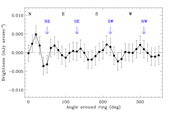
Figure 5: Azimuthal profile of the residual emission after subtracting our best-fit Gaussian model from the 1.3 mm continuum emission. The four clumps discussed by Greaves et al. (2005) and Lestrade & Thilliez (2015) are marked by the blue arrows.

The SMA 1.3 mm data probes structure at higher angular resolution than the previous single dish observations. Moreover, the interferometer naturally provides spatial filtering that serves to highlight the presence of any compact emission peaks. After removing azimuthally symmetric models from the SMA data, any significant azimuthal structure should be readily apparent in the imaged residuals. Figure 5 shows the azimuthal profile of the residual image obtained after subtracting the best-fit Gaussian belt model from the data. Each point represents the mean brightness calculated in a small annular sector with opening angle of $10\arcdeg$ and radial range of $10\arcsec$ to $30\arcsec$. Uncertainties are the image rms noise divided by the square root of the number of beams in each sector. The only potentially significant feature is a peak at $20\arcdeg$, which is visible at the $\sim 4\sigma$ level in the residual images of Figure 3 (right panels). The locations of the previously claimed four clumps (Greaves et al., 2005; Lestrade & Thilliez, 2015) are marked with arrows in Figure 5. While the azimuthal profile of the imaged residuals shows roughly four low significance peaks, these are not aligned well with the previously claimed clumps, and the separations cannot be readily attributed to the previously claimed rotation. However, the signal-to-noise of these residuals is still lacking. The signature of the four clumps discussed in Lestrade & Thilliez (2015), if they do exist, have been weakened in the fitting procedure by using an azimuthally uniform ring as the model. A more definitive statement about low level clumps will require high resolution observations with higher sensitivity.

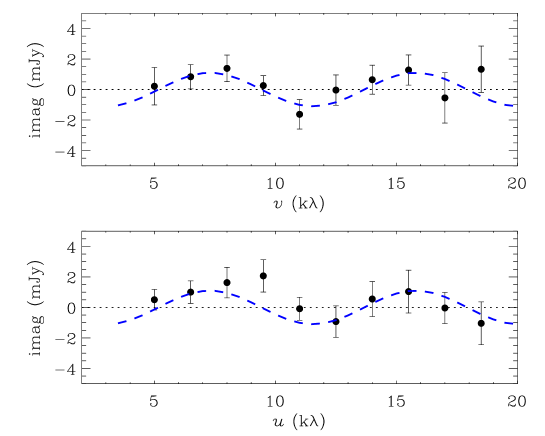
Figure 6: Complex visibilities of the 1.3 mm emission binned along the $v$-axis (top) and the $u$-axis (bottom). Model visibilities generated by inserting a 1 mJy point source at the position of the $4\sigma$ peak seen in the residual map are shown by the blue dashed lines.

The imaginary part of the visibilities is very sensitive to the presence of asymmetries in the emission structure. Indeed, the effect of the marginally significant peak in the residual images is apparent. Figure 6 shows the imaginary part of the visibilities binned along the $u$-axis and along the $v$-axis of the Fourier plane. For a symmetric structure, the imaginary part of the visibilities should be zero; however, both of these views show hints of a low amplitude, sinusoidal oscillation. This structure in the visibilities arises naturally from a single, offset emission peak. The Fourier transform of a point source with amplitude, $A$, offset from the center of the image in the $u$ and $v$ directions by $x_{0}$ and $y_{0}$, respectively, is given by $G(u,v)=A\times\text{exp}[-2\pi(x_{0}u+y_{0}v)]$ (making use of the shift theorem, whereby a shift in the position of a function by an amount $x_{0}$ corresponds to a phase change in its Fourier transform by exp$(i2\pi x_{0}u)$, e.g. Isella et al. (2013)); the imaginary part of this expression is $\mathcal{I}(G(u,v))=A\times\text{sin}[2\pi(x_{0}u+y_{0}v)]$. That is, a point source offset from $(0,0)$ introduces a simple sinusoidal oscillation in the imaginary part of the visibilities. As shown in Figure 6, if we insert a 1 mJy point source at the location of the $4\sigma$ peak in the residual image ($x_{0}\approx 15\arcsec$, $y_{0}\approx 25\arcsec$) into the visibilities, the resulting imaginary visibility curve matches very well the shape and scale of the residuals. Thus, this single residual feature can account for most of the structure in the imaginary visibilities, or most of the detected asymmetry. This feature does not match up with any of the clumps previously identified in single dish images. Also, it is positioned clockwise from the northeast feature, which is not consistent with the counterclockwise rotation suggested by Greaves et al. (2005). The exact nature of this marginally significant peak is uncertain. If it is a background galaxy, then the proper motion of the star will move the debris disk away from it, and this should become evident in interferometric observations at future epochs. An extragalactic source should also appear compact at the arcsecond level. Recent deep ALMA surveys (Hodge et al., 2013; Karim et al., 2013) have built up statistics describing the number counts of submillimeter galaxies expected in a given field of view. At 1.3 mm, the expected number of sources with flux $\geq 1$ mJy expected in the $52\arcsec$ primary beam of the SMA is $0.41^{+0.25}_{-0.15}$ (Ono et al., 2014). Hence the presence of a background submillimeter galaxy in the image at this flux level is not a rare event. Verification and characterization of any asymmetric structure in the millimeter emission from the belt requires observations with higher resolution and sensitivity.

4.1.6 Belt Spectral Index

The long wavelength spectral index of the continuum belt emission reflects the underlying dust opacities and provides a constraint on the size distribution of the emitting grains in the debris disk (Ricci et al., 2012), which can be related to collisional models.

For optically thin dust emission, the flux density is given by $F_{\nu}\propto B_{\nu}(T_{\text{dust}})\kappa_{\nu}M_{\text{dust}}/d^{2}$, where $B_{\nu}(T_{\text{dust}})$ is the Planck function at the dust temperature $T_{\text{dust}}$, $\kappa_{\nu}\propto\nu^{\beta}$ is the dust opacity, expressed as a power law at these long wavelengths, $M_{\text{dust}}$ is the dust mass, and $d$ is the distance. At long millimeter wavelengths, for sufficiently high temperatures, the Planck function reduces to the Rayleigh-Jeans approximation $B_{\nu}(T_{\text{dust}})\propto\nu^{\alpha_{\text{Pl}}}$ with $\alpha_{\text{Pl}}=2$. Thus, $\alpha_{\text{mm}}\approx\alpha_{\text{Pl}}+\beta$, where $\alpha_{\text{mm}}$ is the millimeter spectral index. Draine (2006) derived a relation between $\beta$, the dust opacity power law index, and $q$, the grain size distribution parameter: $\beta\approx(q-3)\beta_{s}$, where $\beta_{s}=1.8\pm 0.2$ is the dust opacity spectral index in the small particle limit for interstellar grain materials, valid for $3<q<4$ and size distributions that follow a power law over a broad enough interval. Combining these relationships provides a simple expression for the slope of the grain size distribution, $q$, as a function of $\alpha_{\text{mm}}$, $\alpha_{\text{Pl}}$, and $\beta_{s}$: $q=(\alpha_{\text{mm}}-\alpha_{\text{Pl}})/\beta_{s}+3$.

For $\epsilon$ Eridani, the fit to the ATCA 7 mm data places an upper limit on the belt flux density of $F_{\text{belt}}<310$ $\mu$Jy ($3\sigma$). Combining this 7 mm limit with the SMA 1.3 mm measurement provides a long lever arm in wavelength that largely overcomes systematic uncertainties and constrains the millimeter spectral index, $\alpha_{\text{mm}}>2.39$. This limit on the spectral index results in a limit on the grain size distribution power-law index $q>3.22$.

The derived limit on the grain size distribution power-law index is consistent with the classical prediction of $q=3.5$ for a steady-state collisional cascade (Dohnanyi, 1969). Ricci et al. (2012) obtained a similar result from analysis of the millimeter spectrum of the Fomalhaut debris disk, $q=3.48\pm 0.14$. This standard collisional cascade assumes that collisions in the disk occur between bodies of identical tensile strength and velocity dispersion, regardless of size. Pan & Schlichting (2012) revisited the theory by relaxing the assumption of a single velocity dispersion and solving self-consistently for a size-dependent velocity distribution in steady-state. This more complex analysis yields steeper size distributions, with $q\approx 4$. Since the $\epsilon$ Eridani spectral index is only a lower limit, a steeper grain size distribution cannot be ruled out. We note that the best-fit value for the 7 mm flux density ($F_{\text{belt}}=110~{}\mu$Jy) yields $q=3.55\pm 0.36$, still shallower than predicted by models with size-dependent velocity dispersions. This result, and the more robust measurement for Fomalhaut, do not support the steeper size distributions predicted by the collisional models with velocity distribution variations. But spectral indices need to be determined for a much larger sample of debris disks to draw a definitive conclusion.

4.2 Central Component

A central source is clearly detected in the SMA 1.3 mm image and ATCA 7 mm image, coincident with the position of the star at the time of observation. The source size is below the resolution limit of these observations, most clearly evidenced by the lack of fall off at long baselines in Figure 4. The 1.3 mm flux density of this source is $F_{\text{cen}}=1.08^{+0.19}_{-0.41}$ mJy. Lestrade & Thilliez (2015) report a similar value in MAMBO-2/IRAM 1.2 mm data, detecting a central source with flux density $1.2\pm 0.3$ mJy. These measurements are only marginally compatible with expectations for the stellar photosphere at these long wavelengths. The effective temperature of $\epsilon$ Eridani is $T_{\text{eff}}=5039\pm 126$ K (Baines & Armstrong, 2012), and a Kurucz stellar atmosphere model (see Backman et al., 2009) predicts a 1.3 mm flux density of 0.53 mJy (with 2% uncertainty). The ATCA 7 mm flux density of this same central source is $F_{\text{cen}}=66.1^{+6.9}_{-10.5}$ $\mu$Jy, substantially in excess of the stellar photoshere model flux prediction of 18 $\mu$Jy. The central source persists at a consistent intensity in all of the 8 days of ATCA observations, showing no significant variability. The mean flux density is $66.5\pm 9.5$ $\mu$Jy and $65.9\pm 7.0$ $\mu$Jy for the June and August observations, respectively.

In principle, the central 1.3 mm excess emission could be explained by thermal dust emission from a warm inner belt. This small 1.3 mm excess, together with Spitzer 24 $\mu$m and Herschel 70 and 160 $\mu$m inner excesses, are consistent with emission from a $70-100$ K blackbody, similar to previous inferences by Backman et al. (2009) and Greaves et al. (2014) from the infrared spectrum alone. For reasonable grain sizes, this blackbody emission corresponds to a (very narrow) inner dust belt at $2-10$ AU, consistent with the size constraint from the SMA observations. However, this same blackbody model produces negligible emission at 7 mm. While previous infrared measurements indicate that there is clearly some warm dust present in the system (unresolved in our observations), no inner dust belt scenario can also match the substantial 7 mm excess from the ATCA observations.

We consider it likely that the unresolved excess emission from the central source arises from an additional stellar component, either an ionized corona or chromosphere. The absence of variability on the month to month timescale suggests a thermal origin. In particular, the millimeter wavelength emission from $\epsilon$ Eridani is reminiscent of the nearby solar-type stars $\alpha$ Cen A and B (spectral types G2V and K2V) recently reported by Liseau et al. (2015) and attributed to heated plasma, similar to the Sun’s chromosphere. Following Liseau et al. (2013), we calculate the Planck brightness temperature for $\epsilon$ Eridani at 1.3 mm and 7 mm, assuming the photospheric radius of the star is sufficiently similar at optical and radio wavelengths to introduce negligible errors. Optical interferometry of $\epsilon$ Eridani gives a precise measure of the stellar radius, $R_{\text{phot}}=0.74\pm 0.01R_{\odot}$ (Baines & Armstrong, 2012). At 1.3 mm, this radius and the excess emission implies $T_{\text{B}}=7800\pm 1400$ K, somewhat higher than the optical effective temperature. At 7 mm, however, $T_{\text{B}}=13000\pm 1600$ K, very much in excess of the photospheric prediction. Indeed, the $\epsilon$ Eridani emission follows the same trend with increasing wavelength as found for $\alpha$ Cen A and B from ALMA observations. Liseau et al. (2015) measure spectral indices between 0.87 mm and 3.1 mm of $1.62$ and $1.61$ for $\alpha$ Cen A and B, respectively. From the SMA and ATCA data, the spectral index of the central component of $\epsilon$ Eridani between 1.3 mm and 7 mm is very similar, $1.65\pm 0.23$ (where we have added in quadrature the $\sim 10\%$ flux scale uncertainties at both wavelengths with the $1\sigma$ errors from model fits). The stellar spectrum clearly starts to deviate strongly from a simple optically thick photosphere with a Rayleigh-Jeans spectral index of 2.0, and the contrast between the photosphere and the putative chromosphere increases at longer wavelengths. While observations of $\epsilon$ Eridani at centimeter wavelengths have so far provided only upper limits, $<80~{}\mu$Jy at 3.6 cm (Gudel, 1992) and $<105~{}\mu$Jy at 6 cm (Bower et al., 2009), much more sensitive observations are now possible with the upgraded Karl G. Jansky Very Large Array, and this would be useful to help constrain the plasma properties.

5 Conclusions

We present SMA 1.3 mm and ATCA 7 mm observations of $\epsilon$ Eridani, the first millimeter interferometric observations of this nearby debris disk system, probing to $4^{\prime\prime}$ (13 AU) scales. These observations resolve the outer dust emission belt surrounding the star, and they reveal a compact emission source coincident with the stellar position. We use MCMC techniques to fit models of the emission structure directly to the visibility data in order to constrain the properties of the two components. The main results are:

1. The outer belt is located precisely and resolved radially. Gaussian and power law emission profiles each fit the SMA 1.3 mm data comparably well. For the best-fit Gaussian model, the belt radial location is $R_{\text{cen}}=64.4^{+2.4}_{-3.0}$ AU and $\text{FWHM}=20.2^{+6.0}_{-8.2}$ AU, corresponding to a fractional belt width $\Delta R/R=0.31^{+0.09}_{-0.13}$. This width is at the high end of inferences from previous single dish millimeter observations, and wider than the classical Kuiper Belt in our Solar System.

2. The outer belt shows no evidence for significant azimuthal structure that might be attributed to gravitational sculpting by planets. After subtracting a symmetric model from the SMA 1.3 mm data, imaging shows only one low significance peak, and its location does not correspond to any clumps identified in previous millimeter and submillimeter observations of $\epsilon$ Eridani. The presence of this feature is consistent with source counts for the extraglactic background in the field of view. In addition, the SMA 1.3 mm data constrains any centroid offset of the belt from the star to $<9$ AU, which limits the presence of giant planet perturbers on wide and eccentric orbits in the system.

3. A central source coincident with the star is clearly detected in both the SMA 1.3 mm image and the ATCA 7 mm image, and the flux densities of this source exceed extrapolations from shorter wavelengths for the stellar photosphere. While the excess is marginal at 1.3 mm, it is highly significant– about a factor of three– at 7 mm. The stellar spectrum clearly departs from an optically thick photosphere at these long wavelengths, with spectral index $1.65\pm 0.23$ between 1.3 mm and 7 mm. This spectrum cannot be explained by an inner warm dust belt and plausibly results from heated plasma in a stellar chromosphere, by analogy with the Sun and $\alpha$ Cen. The high brightness temperature at 7 mm of $13000\pm 1600$ K for a source of stellar size lends additional credence to this conclusion.

4. Combining the SMA 1.3 mm measurement of the belt flux density with the ATCA 7 mm upper limit constrains the spectral index of the emission, $\alpha_{\text{mm}}>2.39$. For conventional assumptions about the dust grains, this spectral index corresponds to a limit on the slope of the power law grain size distribution in the belt, $q>3.22$, consistent with the classical prediction of $q=3.5$ for a self-similar steady-state collisional cascade. This slope is also consistent with the steeper distributions predicted by collisional models that allow for size-dependent velocities and strengths.

These SMA and ATCA millimeter wavelength observations provide the highest resolution view of the outer dust belt surrounding $\epsilon$ Eri at the longest wavelengths to date. But deeper observations are still needed to measure radial gradients in the debris disk and to reveal substructure due to planets, if present, in order to further constrain scenarios for the evolution of planetesimals surrounding this very nearby star.

Appendix A Primary Beam Structure of the SMA

The SMA is composed of eight essentially identical antennas, each 6 meters in diameter. The SMA primary beam is thus the power pattern of one antenna. While the primary beam shape is often assumed to be a simple Gaussian, the actual shape is determined by illumination with a 10 dB taper at the edge of the primary dish, as well as blockage due to the secondary mirror. With these considerations, the beam power as a function of offset (in arcseconds) from the beam center is given by

$$P=\left[\int^{R_{s}}_{R_{p}}2\pi rJ_{0}\left(\frac{2\pi rx}{\lambda}\right)J_{0}\left(\frac{1.840839r}{R_{p}}\right)\right]^{2}$$ (3)

where, $R_{p}$ is the radius of the primary dish in meters, $R_{s}$ is the radius of the secondary dish in meters, and $x$ is the offset from the dish center in radians. A complete profile of the beam power can be built up using Equation 3 at discrete offset positions. Note that this expression does not take into account additional practical factors, such as receiver alignment, pointing jitter, and departures from perfect focus, which act to distort the primary beam shape.

Since the emission extent of the $\epsilon$ Eridani disk is comparable to the half power size of the SMA primary beam pattern, we constructed a complete beam model for use in our modeling procedure. The FWHM of accurate beam models for the LSB (218.9 GHz) and USB (230.9 GHz) are $53\farcs 6$ and $50\farcs 8$, respectively. For comparison, the FWHM for a uniformly illuminated circular aperture antenna is given by $1.22\lambda/D_{A}$, where $D_{A}$ is the antenna diameter. For the SMA antennas, this predicts $50\farcs 4$ and $47\farcs 4$, for the LSB and USB, respectively, narrower than the FWHM of the accurate beam models. Note that tasks within the miriad software package assume a Gaussian beam for the SMA with a FWHM given by a uniformly illuminated circular aperture.

Table 1: Submillimeter Array Observations of $\epsilon$ Eridani

Observation	Array	Projected	HA	225 GHz atm.
Date	Config.	Baselines (m)	Range	Opacity${}^{\text{a}}$
2014 July 28	Subcompact	$6-35$	$-3.6,3.3$	$0.09$
2014 July 29	Subcompact	$6-35$	$-3.7,2.8$	$0.07$
2014 July 30	Subcompact	$6-35$	$-3.5,7.1$	$0.08$
2014 Aug 5	Subcompact	$6-35$	$-3.5,2.2$	$0.12$
2014 Nov 19	Subcompact	$6-56$	$-3.6,4.3$	$0.07$

Note. — ${}^{\text{a}}$ characteristic value for the track measured at the nearby Caltech Submillimeter Observatory. The LO frequency for all observations was 225.5 GHz.

Table 2: Australia Telescope Compact Array Observations of $\epsilon$ Eridani

Observation	Array	Projected	HA	Seeing rms
Date	Config.	Baselines (m)	Range	(microns)${}^{\text{a}}$
2014 June 25	H168	$36-180$	$-3.6,3.6$	$150$
2014 June 26	H168	$36-180$	$-3.6,3.6$	$60$
2014 June 27	H168	$31-180$	$-4.0,3.6$	$70$
2014 June 28	H168	$31-180$	$-4.1,0.0$	$250$
2014 Aug 2	H75	$22-84$	$-4.7,3.9$	$80$
2014 Aug 3	H75	$22-84$	$-4.4,4.0$	$80$
2014 Aug 4	H75	$22-84$	$-4.6,4.0$	$150$
2014 Aug 5	H75	$22-84$	$-3.8,4.0$	$130$

Note. — ${}^{\text{a}}$ characteristic value for the track measured by the ATCA seeing monitor, an interferometer on a 230 m east-west baseline that tracks the 30.48 GHz beacon on the geostationary communications satellite, OPTUS-B3, at an elevation of $60\arcdeg$. (Middelberg et al., 2006). The LO frequency for all observations was 44 GHz.

Table 3: SMA Model Parameters

Parameter	Description	Power Law	Gaussian
		Best-Fit	Best-Fit
$F_{\text{belt}}$	Belt flux density (mJy)	$16.9(+3.9,-5.6)$	$17.2(+5.1,-4.5)$
$F_{\text{cen}}$	Central source flux (mJy)	$1.08(+0.19,-0.41)$	$1.06(+0.34,-0.34)$
$R_{\text{in}}$	Belt inner radius (AU)	$53.4(+6.1,-5.0)$	$-$
$R_{\text{out}}$	Belt outer radius (AU)	$80.2(+3.0,-7.1)$	$-$
$x$	Belt radial power law index	$1.92(+0.18,-2.94)$	$-$
$R_{\text{cen}}$	Belt center radius (AU)	$-$	$64.4(+2.4,-3.0)$
$\sigma$	Belt width (AU)	$-$	$8.55(+2.54,-3.46)$
$i$	Belt inclination $(^{\circ})$	$17.9(+10.2,-15.3)$	$17.3(+14.2,-14.2)$
$PA$	Belt position angle $(^{\circ})$	$3.42(+23.3,-23.4)$	$1.66(+6.70,-6.70)$
$\Delta\alpha$	R.A. offset of belt center $(\arcsec)$	$0.01(+0.65,-1.03)$	$0.02(+0.80,-0.80)$
$\Delta\delta$	Decl. offset of belt center $(\arcsec)$	$1.63(+0.86,-0.86)$	$1.63(+0.70,-1.01)$
$\Delta\alpha_{\text{star}}$	R.A. offset of star from belt center $(\arcsec)$	$-1.18(+0.65,-1.40)$	$-1.22(+0.87,-1.26)$
$\Delta\delta_{\text{star}}$	Decl. offset of star from belt center $(\arcsec)$	$0.11(+0.90,-1.29)$	$0.11(+1.10,-1.10)$

Table 4: ATCA Model Parameters

Parameter	Description	Best-Fit
$F_{\text{belt}}$	Belt flux density ($\mu$Jy)	$110.(+65.,-117.)$
$F_{\text{cen}}$	Central source flux ($\mu$Jy)	$66.1(+6.9,-10.5)$
$\Delta\alpha$	R.A. offset of belt center $(\arcsec)$	$-0.87(+0.72,-0.87)$
$\Delta\delta$	Decl. offset of belt center $(\arcsec)$	$0.38(+0.86,-0.62)$

References

- Anglada-Escudé & Butler (2012) Anglada-Escudé, G., & Butler, R. P. 2012, ApJS, 200, 15
- Aumann (1985) Aumann, H. H. 1985, PASP, 97, 885
- Backman et al. (2009) Backman, D., et al. 2009, ApJ, 690, 1522
- Backman & Paresce (1993) Backman, D. E., & Paresce, F. 1993, in Protostars and Planets III, ed. E. H. Levy & J. I. Lunine, 1253–1304
- Baddour (2009) Baddour, N. 2009, Journal of the Optical Society of America A, 26, 1767
- Baines & Armstrong (2012) Baines, E. K., & Armstrong, J. T. 2012, ApJ, 744, 138
- Boley et al. (2012) Boley, A. C., Payne, M. J., Corder, S., Dent, W. R. F., Ford, E. B., & Shabram, M. 2012, ApJ, 750, L21
- Bower et al. (2009) Bower, G. C., Bolatto, A., Ford, E. B., & Kalas, P. 2009, ApJ, 701, 1922
- Chiang et al. (2009) Chiang, E., Kite, E., Kalas, P., Graham, J. R., & Clampin, M. 2009, ApJ, 693, 734
- Deller & Maddison (2005) Deller, A. T., & Maddison, S. T. 2005, ApJ, 625, 398
- Dohnanyi (1969) Dohnanyi, J. S. 1969, J. Geophys. Res., 74, 2531
- Draine (2006) Draine, B. T. 2006, ApJ, 636, 1114
- Foreman-Mackey et al. (2013) Foreman-Mackey, D., Hogg, D. W., Lang, D., & Goodman, J. 2013, PASP, 125, 306
- Gáspár et al. (2012) Gáspár, A., Psaltis, D., Rieke, G. H., & Özel, F. 2012, ApJ, 754, 74
- Goodman & Weare (2010) Goodman, J., & Weare, J. 2010, Commun. Appl. Math. Comput. Sci., 5, 65
- Greaves et al. (1998) Greaves, J. S., et al. 1998, ApJ, 506, L133
- Greaves et al. (2005) —. 2005, ApJ, 619, L187
- Greaves et al. (2014) —. 2014, ApJ, 791, L11
- Gudel (1992) Gudel, M. 1992, A&A, 264, L31
- Hahn & Malhotra (2005) Hahn, J. M., & Malhotra, R. 2005, AJ, 130, 2392
- Hatzes et al. (2000) Hatzes, A. P., et al. 2000, ApJ, 544, L145
- Ho et al. (2004) Ho, P. T. P., Moran, J. M., & Lo, K. Y. 2004, ApJ, 616, L1
- Hodge et al. (2013) Hodge, J. A., et al. 2013, ApJ, 768, 91
- Isella et al. (2013) Isella, A., Pérez, L. M., Carpenter, J. M., Ricci, L., Andrews, S., & Rosenfeld, K. 2013, ApJ, 775, 30
- Janson et al. (2015) Janson, M., Quanz, S. P., Carson, J. C., Thalmann, C., Lafrenière, D., & Amara, A. 2015, A&A, 574, A120
- Karim et al. (2013) Karim, A., et al. 2013, MNRAS, 432, 2
- Kennedy & Wyatt (2010) Kennedy, G. M., & Wyatt, M. C. 2010, MNRAS, 405, 1253
- Kenyon & Bromley (2008) Kenyon, S. J., & Bromley, B. C. 2008, ApJS, 179, 451
- Kuchner & Holman (2003) Kuchner, M. J., & Holman, M. J. 2003, ApJ, 588, 1110
- Kuchner & Stark (2010) Kuchner, M. J., & Stark, C. C. 2010, AJ, 140, 1007
- Lay et al. (1997) Lay, O. P., Carlstrom, J. E., & Hills, R. E. 1997, ApJ, 489, 917
- Lestrade & Thilliez (2015) Lestrade, J.-F., & Thilliez, E. 2015, ArXiv e-prints
- Liseau et al. (2013) Liseau, R., et al. 2013, A&A, 549, L7
- Liseau et al. (2015) —. 2015, A&A, 573, L4
- MacGregor et al. (2015) MacGregor, M. A., Wilner, D. J., Andrews, S. M., & Hughes, A. M. 2015, ApJ, 801, 59
- MacGregor et al. (2013) MacGregor, M. A., et al. 2013, ApJ, 762, L21
- Mamajek & Hillenbrand (2008) Mamajek, E. E., & Hillenbrand, L. A. 2008, ApJ, 687, 1264
- Matthews et al. (2014) Matthews, B. C., Krivov, A. V., Wyatt, M. C., Bryden, G., & Eiroa, C. 2014, Protostars and Planets VI, 521
- Middelberg et al. (2006) Middelberg, E., Sault, R. J., & Kesteven, M. J. 2006, PASA, 23, 147
- Ono et al. (2014) Ono, Y., Ouchi, M., Kurono, Y., & Momose, R. 2014, ApJ, 795, 5
- Pan & Schlichting (2012) Pan, M., & Schlichting, H. E. 2012, ApJ, 747, 113
- Quillen (2006) Quillen, A. C. 2006, MNRAS, 372, L14
- Reid et al. (1988) Reid, M. J., Schneps, M. H., Moran, J. M., Gwinn, C. R., Genzel, R., Downes, D., & Roennaeng, B. 1988, ApJ, 330, 809
- Reidemeister et al. (2011) Reidemeister, M., Krivov, A. V., Stark, C. C., Augereau, J.-C., Löhne, T., & Müller, S. 2011, A&A, 527, A57
- Ricci et al. (2015) Ricci, L., Carpenter, J. M., Fu, B., Hughes, A. M., Corder, S., & Isella, A. 2015, ApJ, 798, 124
- Ricci et al. (2012) Ricci, L., Testi, L., Maddison, S. T., & Wilner, D. J. 2012, A&A, 539, L6
- Schütz et al. (2004) Schütz, O., Nielbock, M., Wolf, S., Henning, T., & Els, S. 2004, A&A, 414, L9
- van Leeuwen (2007) van Leeuwen, F. 2007, A&A, 474, 653
- Wilson et al. (2011) Wilson, W. E., et al. 2011, MNRAS, 416, 832
- Wyatt (2003) Wyatt, M. C. 2003, ApJ, 598, 1321
- Wyatt (2006) —. 2006, ApJ, 639, 1153
- Wyatt (2008) —. 2008, ARA&A, 46, 339
- Wyatt et al. (1999) Wyatt, M. C., Dermott, S. F., Telesco, C. M., Fisher, R. S., Grogan, K., Holmes, E. K., & Piña, R. K. 1999, ApJ, 527, 918