We complement the analysis of the anomalous top–Higgs coupling effects on the secondary lepton distributions in the associated production of the top-quark pair and Higgs boson in proton–proton collisions at the LHC of the former work by one of the present authors by taking into account the quark–antiquark production mechanism. We also present simple arguments which explain why the effects of the scalar and pseudoscalar anomalous couplings on the unpolarized cross section of the process are completely insensitive to the sign of either of them.

1 Introduction

Determination of the coupling of the recently discovered Higgs boson [1] to the top quark currently belongs to one of the most challenging tasks of the high energy experimental physics. Measurement of the associated production of the top quark pair and Higgs boson in the clean experimental environment of $e^{+}e^{-}$ collisions was considered in this context already more than two decades ago [2], [3], but different projects of the high energy $e^{+}e^{-}$ collider [4]–[11], despite some of them being more or less intensively discussed for years, are still at a rather early stage of TDR. However, if the LHC performance in next runs is as excellent as it was in run 1 we may expect that the process

$$pp\;\rightarrow\;t\bar{t}H$$ (1)

the search for which, based on run 1 data, were already reported by both the CMS [12] and ATLAS [13] collaborations, will be measured quite precisely. This is why in the past few years the associated production of the top quark pair and Higgs boson has invoked quite some interest also from a theoretical side, see, e.g., [14]–[21].

It was shown in Ref. [15] that the distributions in rapidity and angles of the secondary lepton that can be produced in the decay of $\bar{t}$-quark of process (1) are quite sensitive to modifications of the top–Higgs coupling. Actually, only the gluon fusion mechanism of $t\bar{t}H$ production, which is dominant at the LHC energies, and one specific decay channel: $t\to bW^{+}\to bu\bar{d}$, $\bar{t}\to\bar{b}W^{-}\to\bar{b}\mu^{-}\bar{\nu}_{\mu}$ and $h\to b\bar{b}$, were taken into account in Ref. [15], i.e., the following hard parton scattering processes

$$gg\;\rightarrow\;bu\bar{d}\,\bar{b}\mu^{-}\bar{\nu}_{\mu}b\bar{b},$$ (2)

was considered. There are $67\,300$ Feynman diagrams of process (2) already in the leading order (LO) of the standard model (SM) in the unitary gauge, if the Cabibbo-Kobayashi-Maskawa mixing and masses smaller than the $b$-quark mass $m_{b}$ are neglected. At the same time there are only 32 Feynman diagrams which contribute to the signal cross section of $t\bar{t}H$ production, two of which are shown in Fig. 1. The remaining 30 signal diagrams are obtained from those depicted by attaching the Higgs boson line of $Hb\bar{b}$-vertex to the other $t$- or $\bar{t}$-quark line, or interchanging the $b$ and $\bar{b}$ quarks in Figs. 1(a) and 1(b) and interchanging the two gluons in Fig. 1(b). The diagrams with the Higgs boson line of $Hb\bar{b}$-vertex attached to either the $b$- or $\bar{b}$-quark line are not counted here, as their contribution to the $t\bar{t}H$ production signal is suppressed by the mass ratio $m_{b}/m_{t}$. The effects caused by modifications of the scalar and pseudoscalar couplings of the Higgs boson to top quark were clearly visible in the $t\bar{t}H$ production signal cross section, but they were to large degree obscured by the interference of the $t\bar{t}H$ production signal diagrams with the diagrams of irreducible off resonance background.

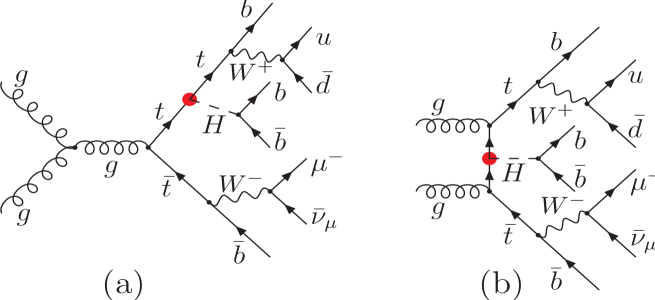
Figure 1: Feynman diagrams of $t\bar{t}H$ production in process (2). Blobs indicate the Higgs–top coupling.

In the present work, we complement the analysis of the influence of the anomalous Higgs boson coupling to top quark on the secondary lepton distributions in the process of associated production of the top quark pair and Higgs boson in proton–proton collisions at the LHC of Ref. [15] by taking into account the quark–antiquark annihilation hard scattering processes with the same final state as that of process (2):

$$q\bar{q}\;\to\;bu\bar{d}\,\bar{b}\mu^{-}\bar{\nu}_{\mu}b\bar{b},$$ (3)

with $q=u,d$. To be more specific, we take into account $u\bar{u}$-, $\bar{u}u$-, $d\bar{d}$- and $\bar{d}d$-scattering processes. Under the same assumptions as those made above for process (2), there are $78\,068$ Feynman diagrams in the LO of SM for each of the $q\bar{q}$-scattering processes considered. However, only $24$ of them contribute to the signal of the $t\bar{t}H$ production. Examples of the signal diagrams of the process of $u\bar{u}$-scattering to the final state of process (3) are shown in Fig. 2.

Figure 2: Feynman diagrams of $t\bar{t}H$ production in the process $u\bar{u}\;\to\;bu\bar{d}\bar{b}\mu^{-}\bar{\nu}_{\mu}b\bar{b}$. Blobs indicate the Higgs–top coupling.

The other signal diagrams can be obtained by attaching the Higgs boson line of the $Hb\bar{b}$-vertex to the other $t$- or $\bar{t}$-quark line or interchanging the $b$- and $\bar{b}$-quark lines in the diagrams of Fig. 2. Let us note that another $24$ diagrams which contain the Feynman propagators of the $t$-, $\bar{t}$-quark and the Higgs boson at a time can be obtained from the signal diagrams just described by the exchange of the $u$-quark lines between the initial and final state. However, they are not treated as the signal diagrams here, because they contain the gluon, $Z^{0}$ or photon propagator in the $t$- or $u$-channel and their contribution to the signal cross section is negligible anyway, which has been checked by direct computation.

The rest of the article is organized in the following way. The possible effect of the anomalous top–Higgs coupling on the unpolarized cross section of the process of $t\bar{t}H$ production at the LHC are analyzed in Section 2, our results are presented in Section 3 and, finally, some concluding remarks are contained in Section 4.

2 Effects of the anomalous top–Higgs coupling

The most general top–Higgs coupling is given by the following Lagrangian [22]:

$$\mathcal{L}_{t\bar{t}H}=-g_{t\bar{t}H}\bar{t}(f+if^{\prime}\gamma_{5})th,$$ (4)

where $g_{t\bar{t}H}=m_{t}/v$, with $v=(\sqrt{2}G_{F})^{-1/2}\simeq 246$ GeV, is the top–Higgs Yukawa coupling and the real couplings $f$ and $f^{\prime}$ describe, respectively, the scalar and pseudoscalar departures from the purely scalar top–Higgs Yukawa coupling of SM, which is reproduced for $f=1$ and $f^{\prime}=0$. The allowed regions of the $(f,f^{\prime})$ plane, according to the analysis of Ref. [16] performed at the 68 and 95% confidence level, are plotted in Fig. 1 of Ref. [17]. They are derived from the constraints on the $Hgg$ and $H\gamma\gamma$ couplings from the Higgs boson production and its decay into $\gamma\gamma$, which among others involve assumptions on the Higgs boson couplings to other fermions and bosons, and hence are model dependent. Therefore, we will not stick to them in the next section, where we will illustrate the effects of $f^{\prime}$ on the process of associated production of the top quark pair and Higgs boson from which the direct constraints on $f$ and $f^{\prime}$ can be derived.

Let us try to predict the possible effect of the top–Higgs coupling given by Eq. (4) on the unpolarized cross section of the process $u\bar{u}\;\to\;bu\bar{d}\bar{b}\mu^{-}\bar{\nu}_{\mu}b\bar{b}$. To this end, let us consider the amplitudes of two dominant diagrams of the $t\bar{t}H$ production: $M_{a}^{(1)}$ of the diagram depicted in Fig. 2(a) and $M_{a}^{(2)}$ of the diagram obtained from that of Fig. 2(a) by attaching the Higgs boson line to the $\bar{t}$-quark. They have the following form:

$$M_{a}^{(1)} = g_{t\bar{t}H}h\,\bar{u}(f+if^{\prime}\gamma_{5})\;\frac{p_{t}\!\!\!\!/+q\!\!\!/+M}{(p_{t}+q)^{2}-M^{2}}\;g_{s}\varepsilon\!\!\!/\,v,$$ (5)

$$M_{a}^{(2)} = g_{t\bar{t}H}h\,\bar{u}g_{s}\varepsilon\!\!\!/\;\frac{-p_{\bar{t}}\!\!\!\!/-q\!\!\!/+M}{(p_{\bar{t}}+q)^{2}-M^{2}}\;(f+if^{\prime}\gamma_{5})\,v,$$ (6)

where $h$ is a scalar representing a product of the Higgs boson propagator carrying the four momentum $q$ with the $Hb\bar{b}$-vertex, $u$ ($v$) is the Dirac spinor representing the off-shell $t$-quark ($\bar{t}$-quark) of the four momentum $p_{t}$ ($p_{\bar{t}}$) that decays into the $b$-quark ($\bar{b}$-quark) and off-shell $W^{+}$ ($W^{-}$)-boson, $\varepsilon$ is a polarization four vector representing the gluon propagator contracted with the $u\bar{u}g$-vertex, $g_{s}$ is the strong coupling constant and $M=\sqrt{m_{t}^{2}-im_{t}\Gamma_{t}}\approx m_{t}-\frac{i}{2}\Gamma_{t}$ is a complex mass parameter that replaces the mass $m_{t}$ in the top quark propagator in order to regularize the pole arising if its denominator approaches zero. After some simple algebra Eqs. (5) and (6) can be written in the following form:

$$M_{a}^{(1)} = \frac{g_{t\bar{t}H}g_{s}h}{(p_{t}+q)^{2}-M^{2}}\left[f\bar{u}(p_{t}\!\!\!\!/+M)\varepsilon\!\!\!/v+if^{\prime}\bar{u}(-p_{t}\!\!\!\!/+M)\gamma_{5}\,\varepsilon\!\!\!/v+\bar{u}(f+if^{\prime}\gamma_{5})q\!\!\!/\varepsilon\!\!\!/v\right],$$ (7)

$$M_{a}^{(2)} = \frac{g_{t\bar{t}H}g_{s}h}{(p_{\bar{t}}+q)^{2}-M^{2}}\left[f\bar{u}\,\varepsilon\!\!\!/(-p_{\bar{t}}\!\!\!\!/+M)v+if^{\prime}\bar{u}\varepsilon\!\!\!/\gamma_{5}(p_{\bar{t}}\!\!\!\!/+M)v-\bar{u}\varepsilon\!\!\!/q\!\!\!/(f+if^{\prime}\gamma_{5})v\right].$$ (8)

Now, let us note that, as in the process of $t\bar{t}H$ production in $e^{+}e^{-}$ collisions that was considered in Ref. [14], the dominant contribution to the cross section comes from the phase space region, where both the $t$-quark and $\bar{t}$-quark are close to their mass shells and hence the off-shell spinors $u$ and $v$ should satisfy the following approximate equations:

$$\bar{u}(p_{t}\!\!\!\!/-m_{t})\approx 0, \qquad\bar{u}(p_{t}\!\!\!\!/+m_{t})\approx 2m_{t},$$ (9)

$$(p_{\bar{t}}\!\!\!\!/+m_{t})v\approx 0, \qquad(p_{\bar{t}}\!\!\!\!/-m_{t})v\approx-2m_{t}.$$ (10)

Using Eqs. (9) in (7) and (10) in (8), and neglecting terms $\sim\Gamma_{t}$ in the numerators, we get the following approximate expressions for the amplitudes:

$$M_{a}^{(1)} \approx c\left[2m_{t}f\bar{u}\varepsilon\!\!\!/v+\bar{u}(f+if^{\prime}\gamma_{5})q\!\!\!/\varepsilon\!\!\!/v\right],\qquad{\rm with}\qquad c=\frac{g_{t\bar{t}H}g_{s}h}{(p_{t}+q)^{2}-M^{2}},$$ (11)

$$M_{a}^{(2)} \approx \bar{c}\left[2m_{t}f\bar{u}\varepsilon\!\!\!/v-\bar{u}\varepsilon\!\!\!/q\!\!\!/(f+if^{\prime}\gamma_{5})v\right],\qquad{\rm with}\qquad\bar{c}=\frac{g_{t\bar{t}H}g_{s}h}{(p_{\bar{t}}+q)^{2}-M^{2}}$$ (12)

and for a sum of the two:

$$M_{a}=M_{a}^{(1)}+M_{a}^{(2)}\approx(c+\bar{c})\left[2m_{t}f\bar{u}\varepsilon\!\!\!/v-\bar{u}\varepsilon\!\!\!/q\!\!\!/(f+if^{\prime}\gamma_{5})v\right]+c\;2q\cdot\varepsilon\bar{u}(f+if^{\prime}\gamma_{5})v.$$ (13)

In order to calculate the sum over polarizations of the squared module of the matrix element $\sum_{\rm pol.}\left|M_{a}\right|^{2}$, we take into account the approximate completeness relations for the spinors $u$ and $v$:

$$\sum_{\rm pol.}u\otimes\bar{u}\approx p_{t}\!\!\!\!/+m_{t},\qquad\sum_{\rm pol.}v\otimes\bar{v}\approx p_{\bar{t}}\!\!\!\!/-m_{t}.$$ (14)

and note that the off-shell polarization four vectors $\varepsilon$ are real, as they are defined in the following way:

$$\varepsilon^{\mu}\equiv\frac{-g^{\mu\nu}}{(p_{1}+p_{2})^{2}}g_{s}\bar{v}(\vec{p}_{1},\lambda_{1})\gamma_{\nu}u(\vec{p}_{2},\lambda_{2}),$$ (15)

where the helicity spinors $v(\vec{p}_{1},\lambda_{1})$ and $u(\vec{p}_{2},\lambda_{2})$ of, respectively, the $\bar{u}$- and $u$-quark in initial state, which are calculated according to Eqs. (5) and (6) of Ref. [25], are real if the momenta $\vec{p}_{1}$ and $\vec{p}_{2}$ are antiparallel. Thus

$$\sum_{\rm pol.}\left|M_{a}\right|^{2} \approx \left|(c+\bar{c})\right|^{2}\left\{4m_{t}^{2}f^{2}{\rm Tr}[(p_{\bar{t}}\!\!\!\!/-m_{t})\varepsilon\!\!\!/(p_{t}\!\!\!\!/+m_{t})\varepsilon\!\!\!/]\right.$$ (16)

$$\qquad\qquad+{\rm Tr}[(p_{\bar{t}}\!\!\!\!/-m_{t})(f+if^{\prime}\gamma_{5})q\!\!\!/\varepsilon\!\!\!/(p_{t}\!\!\!\!/+m_{t})\varepsilon\!\!\!/q\!\!\!/(f+if^{\prime}\gamma_{5})]$$

$$\qquad\qquad-\left.4m_{t}f{\rm Re}{\rm Tr}[(p_{\bar{t}}\!\!\!\!/-m_{t})\varepsilon\!\!\!/(p_{t}\!\!\!\!/+m_{t})\varepsilon\!\!\!/q\!\!\!/(f+if^{\prime}\gamma_{5})]\right\}$$

$$+ 4|c|^{2}(q\cdot\varepsilon)^{2}{\rm Tr}[(p_{\bar{t}}\!\!\!\!/-m_{t})(f+if^{\prime}\gamma_{5})(p_{t}\!\!\!\!/+m_{t})(f+if^{\prime}\gamma_{5})]$$

$$+ 4(q\cdot\varepsilon){\rm Re}\left\{c^{*}(c+\bar{c})\left[2m_{t}f{\rm Tr}[(p_{\bar{t}}\!\!\!\!/-m_{t})(f+if^{\prime}\gamma_{5})(p_{t}\!\!\!\!/+m_{t})\varepsilon\!\!\!/]\right.\right.$$

$$\left.\left.\qquad\qquad-{\rm Tr}[(p_{\bar{t}}\!\!\!\!/-m_{t})(f+if^{\prime}\gamma_{5})(p_{t}\!\!\!\!/+m_{t})\varepsilon\!\!\!/q\!\!\!/(f+if^{\prime}\gamma_{5})]\right]\right\}.$$

More simplified analytic form of Eq. (16) is irrelevant, as the calculation of the cross section will be performed numerically anyway, but let us note that only the terms on the r.h.s. of Eq. (16) that contain $\gamma_{5}$ may be proportional to the product $ff^{\prime}$. However, if we use the relation $\varepsilon\!\!\!/p_{t}\!\!\!\!/\,\varepsilon\!\!\!/=-\varepsilon^{2}p_{t}\!\!\!\!/+2(p_{t}\cdot\varepsilon)\varepsilon\!\!\!/$ in the second and third term and the relation $q\!\!\!/p_{t}\!\!\!\!/\,q\!\!\!/=-q^{2}p_{t}\!\!\!\!/+2(p_{t}\cdot q)q\!\!\!/$ in the second term, and then use the relation

$${\rm Tr}[p_{\bar{t}}\!\!\!\!/\;(f+if^{\prime}\gamma_{5})p_{t}\!\!\!\!/\;\varepsilon\!\!\!/q\!\!\!/(f+if^{\prime}\gamma_{5})]=(f^{2}+f^{\prime 2}){\rm Tr}[p_{\bar{t}}\;\!\!\!\!/p_{t}\!\!\!\!/\;\varepsilon\!\!\!/q\!\!\!/],$$ (17)

in the last term on the r.h.s. of Eq. (16), we see that the dependence on $ff^{\prime}$, and thus a sensitivity to the sign of either $f$ or $f^{\prime}$, disappears in the unpolarized cross section of the hard scattering process $u\bar{u}\;\to\;bu\bar{d}\bar{b}\mu^{-}\bar{\nu}_{\mu}b\bar{b}$. Let us note, that the same arguments can be easily repeated for the amplitudes of the Feynman diagrams of Fig. 1, which dominate the $t\bar{t}H$ production through the gluon fusion process (2). We would like to stress here that all the above approximations are used for the sake of the argument in this section only and are not used to obtain the full results presented in Section 3.

3 Results

The calculation is performed in the framework of the SM, supplemented with the top–Higgs coupling derived from Lagrangian (4), with the use of carlomat [23], a general purpose program for the MC computation of the lowest order cross sections. The differential cross section of the process

$$pp\to bu\bar{d}\,\bar{b}\mu^{-}\bar{\nu}_{\mu}b\bar{b}$$ (18)

is calculated with the use of the following factorization formula

$$d\sigma_{pp\to bu\bar{d}\,\bar{b}\mu^{-}\bar{\nu}_{\mu}b\bar{b}}(s)=\sum_{i,j}\int dx_{1}dx_{2}\>f_{i}(x_{1},Q^{2})\>f_{j}(x_{2},Q^{2})\>d\sigma_{ij\to bu\bar{d}\,\bar{b}\mu^{-}\bar{\nu}_{\mu}b\bar{b}}(s^{\prime}),$$ (19)

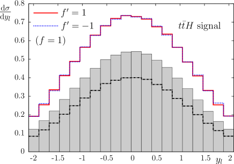
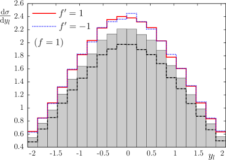
Figure 3: The differential cross section in fb of process (18) at $\sqrt{s}=14$ TeV as a function of the lepton rapidity computed with the $t\bar{t}H$ signal diagrams (left panel) and with all the LO diagrams (right panel). The SM cross section is plotted with grey shaded boxes and the contribution of the gluon fusion to it with the dashed-dotted line and the cross sections in the presence of the anomalous pseudoscalar coupling $f^{\prime}=1$ ($f^{\prime}=-1$) are plotted with the solid (dotted) line.

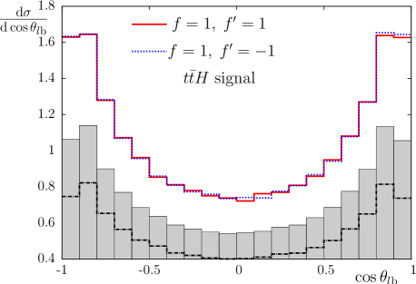
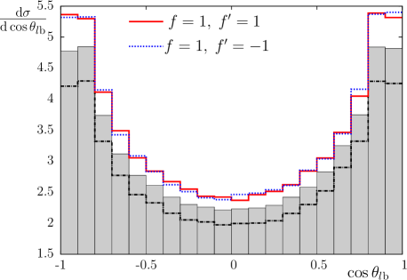
Figure 4: Same as Fig. 3 but as a function of the cosine of the lepton angle with respect to the beam.

where $x_{1}$ and $x_{2}$ are the proton momentum fractions carried by partons $i$ and $j$, respectively, $s^{\prime}=x_{1}x_{2}s$ is the reduced center of mass energy squared, $Q$ is the factorization scale and we take into account the following pairs of partons $(i,j)$: $(g,g)$, $(u,\bar{u})$, $(\bar{u},u)$, $(d,\bar{d})$, $(\bar{d},d)$ in the sum. We use MSTW LO parton distribution functions [24] at the factorization scale $Q=\sqrt{m_{t}^{2}+\sum_{j}p_{Tj}^{2}}$, where $p_{Tj}$ is the transverse momentum of the final state quark or antiquark of process (18). The calculation is performed separately for the gluon fusion (2) and each of the quark–antiquark hard scattering processes (3). We use the same physical input parameters and cuts (3.2)–(3.7), with $m_{bb}^{\rm cut}=20$ GeV in (3.7), as in Ref. [15], and three different combinations of the scalar and pseudoscalar couplings of Lagrangian (4): $(f,f^{\prime})=(1,0),(1,1),(1,-1)$. The first combination corresponds to the SM and the other two are chosen, just for the sake of illustration, beyond the allowed 95% CL regions of the $(f,f^{\prime})$ plane which, as discussed in the first paragraph of Section 2, are model dependent anyway. The cross sections of the hard scattering processes considered are added afterwards, if necessary.

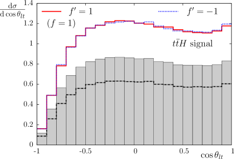
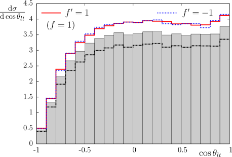
Figure 5: Same as Fig. 3 but as a function of the cosine of the lepton angle with respect to the top quark in the top quark rest frame.

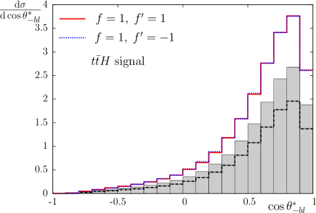
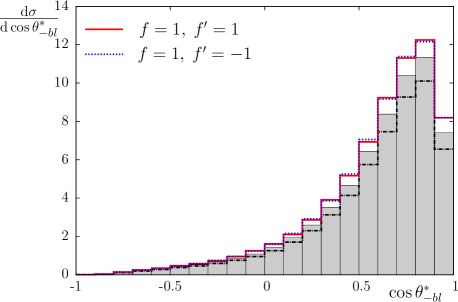
Figure 6: Same as Fig. 3 but as a function of the cosine of the lepton angle with respect to the inverse momentum of the $b$-quark in the top quark rest frame.

Let us note, that in order to calculate the total cross section of process (18), a 20-fold phase space integral and a 2-fold integral over parton density functions must be performed, not to mention the additional 9-fold Monte Carlo (MC) integral that replaces the sum over particle helicities, without which the computation would not have been feasible in practice.

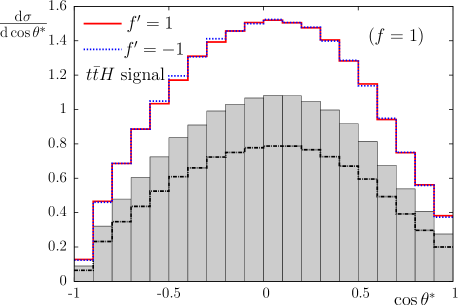
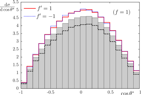
Figure 7: Same as Fig. 3 but as a function of the cosine of the lepton angle with respect to the inverse momentum of the $b$-quark in the $W^{-}$ boson rest frame.

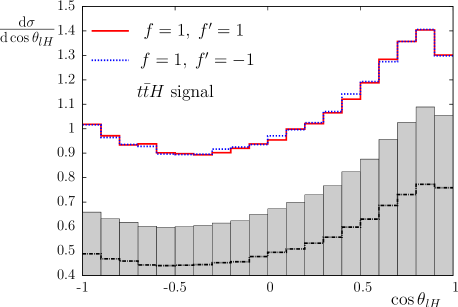
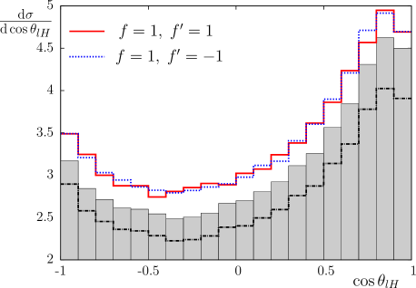
Figure 8: Same as Fig. 3 but as a function of the cosine of the lepton angle with respect to the Higgs boson in the LAB frame.

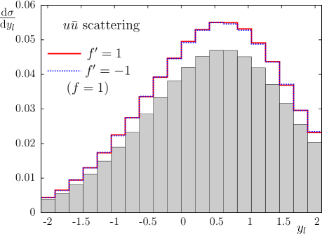
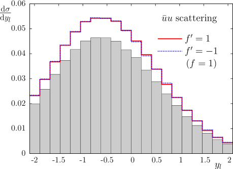
Figure 9: The differential cross section in fb of process (18) at $\sqrt{s}=14$ TeV as a function of the lepton rapidity computed with the $t\bar{t}H$ signal diagrams of the $u\bar{u}$- (left panel) and $\bar{u}u$-hard-scattering processes (right panel). The corresponding SM cross section is plotted with grey shaded boxes.

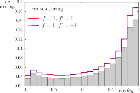
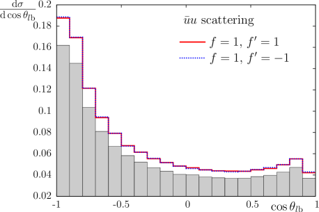
Figure 10: Same as Fig. 9 but as a function of the cosine of the lepton angle with respect to the beam.

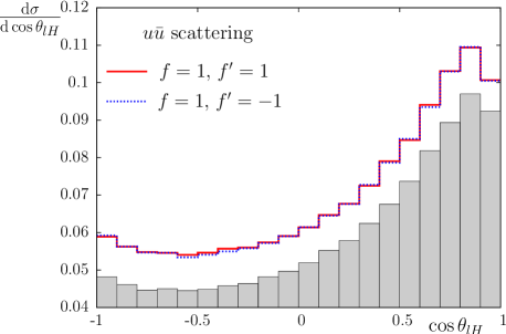
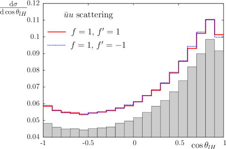
Figure 11: Same as Fig. 9 but as a function of the cosine of the lepton angle with respect to the Higgs boson in the LAB frame.

The differential cross sections of process (18) at the proton–proton center of mass energy of 14 TeV are plotted in Figs. 3–8 as functions of the rapidity and different angular variables of the final state muon, being referred to as the lepton. In Figs. 3–8, the left panels show the signal cross sections, which are computed with the signal $t\bar{t}H$ production diagrams of the hard scattering processes (2) and (3), as described in the previous sections, and the right panels show the complete LO cross sections, which are computed with the complete set of the LO Feynman diagrams of each of the hard scattering processes considered. In each of the figures, the SM cross section of process (18) is plotted with grey shaded boxes and the contribution of the gluon fusion to it with the dashed-dotted line and the cross sections in the presence of the anomalous pseudoscalar coupling $f^{\prime}=1$ ($f^{\prime}=-1$) are plotted with the solid (dotted) line. Thus, the shaded area above the dashed-dotted line shows the contribution of the quark–antiquark hard scattering processes to either the $t\bar{t}H$ signal or complete SM cross section. The effects of the anomalous pseudoscalar coupling $f^{\prime}=\pm 1$ are quite sizable in the signal cross sections which become by about 50% bigger than in the SM. If all the LO Feynman diagrams are taken into account the effects remain the same in absolute terms, but their relative size is substantially smaller, as the anomalous top–Higgs coupling (4) practically does not alter the off resonance background contributions which substantially increase the cross section of process (18). The shape of each of the differential cross sections plotted in Figs. 3–8 is hardly changed in the presence of the anomalous coupling $f^{\prime}=\pm 1$. Moreover, the cross sections for $f^{\prime}=1$ and $f^{\prime}=-1$ look almost identical, which means that the process is practically insensitive to a sign of $f^{\prime}$, in accordance with the discussion of Section 2.

The individual contributions of the $u\bar{u}$- and $\bar{u}u$-hard-scattering processes to the $t\bar{t}H$ signal differential cross sections of process (18) at $\sqrt{s}=14$ TeV are plotted in Figs. 9, 10 and 11, as functions of the lepton rapidity, cosine of the lepton angle with respect to the beam and cosine of the lepton angle with respect to the Higgs boson in the laboratory (LAB) frame, respectively. The relative effects of the anomalous pseudoscalar coupling $f^{\prime}$ in the plots of Figs. 9, 10 and 11 are approximately the same as in the full signal cross sections plotted in the right panels of Figs. 3, 4 and 8, respectively, and again there is practically no sensitivity to the sign of $f^{\prime}$. Taking into account the off resonance background contributions to any of the quark–antiquark hard scattering processes does not change this conclusion either, i. e., the shapes and relative effect of the anomalous coupling $f^{\prime}$ remain practically the same for all the distributions considered.

4 Conclusions

We have complemented the analysis of the influence of the anomalous Higgs boson coupling to top quark on the secondary lepton distributions in the process of associated production of the top quark pair and Higgs boson in the proton–proton collisions at the LHC of Ref. [15] by taking into account contributions of the quark–antiquark annihilation hard scattering processes. Although, the gluon fusion mechanism dominates the $t\bar{t}H$ production through process (18) at $\sqrt{s}=14$ TeV, the contribution of quark–antiquark hard scattering processes (3) is quite substantial and, therefore, should be taken into account in the analyses of data. Moreover, we have explained why the effects of the scalar and pseudoscalar anomalous couplings in the unpolarized cross section of the process are completely insensitive to the sign of either of them.

References

-
[1]
G. Aad et al. [ATLAS collaboration],
Phys. Lett. B 716 (2012) 1 [arXiv:1207.7214 [hep-ex]];
S. Chatrchyan et al. [CMS collaboration], Phys. Lett. B 716 (2012) 30 [arXiv:1207.7235 [hep-ex]]. - [2] A. Djouadi, J. Kalinowski, P.M. Zerwas, Mod. Phys. Lett. A 7 (1992) 1765.
- [3] A. Djouadi, J. Kalinowski, P.M. Zerwas, Z. Phys. C 54 (1992) 255.
- [4] James Brau, Yasuhiro Okada, Nicholas Walker, et al. [ILC collaboration], ILC reference design report: ILC global design effort and world wide study, arXiv:0712.1950 [physics.acc-ph].
- [5] J.A. Aguilar-Saavedra et al. [ECFA/DESY LC Physics Working Group Collaboration], TESLA: the superconducting electron positron linear collider with an integrated x-ray laser laboratory. Technical design report. Part 3. Physics at an linear collider, arXiv:hep-ph/0106315.
- [6] T. Abe et al., [American Linear Collider Working Group collaboration], Linear collider physics resource book for Snowmass 2001 – Part 2: Higgs and supersymmetry studies, arXiv:hep-ex/0106056.
- [7] K. Abe et al. [ACFA Linear Collider Working Group collaboration], Particle physics experiments at JLC, arXiv:hep-ph/0109166.
- [8] CLIC Study <http://clic-study.web.cern.ch/clic-study/>.
- [9] FCC-ee design study, <http://tlep.web.cern.ch/>.
- [10] M. Ahmad et al. [CEPC-SPPC Study Group], CEPC-SPPC Preliminary Conceptual Design Report: Volume I - Physics and Detector, <http://cepc.ihep.ac.cn/preCDR/volume.html>.
- [11] A. Apyan et al. [CEPC-SPPC Study Group], CEPC-SPPC Preliminary Conceptual Design Report: Volume II - Accelerator, <http://cepc.ihep.ac.cn/preCDR/volume.html>.
- [12] CMS Collaboration, JHEP 09 (2014) 087 [arXiv:1408.1682 [hep-ex]].
-
[13]
ATLAS Collaboration,
ATLAS-CONF-2015-007;
ATLAS Collaboration, arXiv:1503.05066 [hep-ex]. -
[14]
K. Kołodziej, S. Szczypiński, Acta Phys. Pol. B 38 (2007) 2565
[hep-ph/0612183];
K. Kołodziej, S. Szczypiński, Nucl. Phys. B 801 (2008) 153 [arXiv:0803.0887 [hep-ph]];
K. Kołodziej, S. Szczypiński, Eur. Phys. J. C 64 (2009) 645 [arXiv:0903.4606 [hep-ph]]. - [15] K. Kołodziej, JHEP 07 (2013) 083 [arXiv:1303.4962 [hep-ph]].
- [16] J. Ellis and T. You, JHEP 06 (2013) 103 [arXiv:1303.3879 [hep-ph]].
- [17] J. Ellis, D.S. Hwang, K. Sakurai, M. Takeuchi, JHEP 04 (2014) 004 [arXiv:1312.5736 [hep-ph]].
- [18] F. Demartin, F. Maltoni, K. Mawatari, B. Page, M. Zaro, Eur. Phys. J. C74 (2014) 3065 [arXiv:1407.5089 [hep-ph]].
- [19] F. Maltoni, D. Pagani, I. Tsinikos, arXiv:1507.05640 [hep-ph].
- [20] S. Khatibi, M.M. Najafabadi, Phys. Rev. D 90 (2014) 074014 [arXiv:1409.6553 [hep-ph]].
- [21] M.R. Buckley, D. Goncalves, arXiv:1507.07926 [hep-ph].
- [22] J.A. Aguilar-Saavedra, Nucl. Phys. B 821 (2009) 215 [arXiv:0904.2387 [hep-ph]].
- [23] K. Kołodziej, Comput. Phys. Commun. 185 (2014) 323 [arXiv:1305.5096 [hep-ph]].
- [24] A.D. Martin, W.J. Stirling, R. S. Thorne, G. Watt, Eur. Phys. J. C 63 (2009) 189-285 [arXiv:0901.0002].
- [25] F. Jegerlehner, K. Kołodziej, Eur. Phys. J. C 12 (2000) 77.