Unified functional network and nonlinear time series analysis for complex systems science: The pyunicorn package

Abstract

We introduce the pyunicorn (Pythonic unified complex network and recurrence analysis toolbox) open source software package for applying and combining modern methods of data analysis and modeling from complex network theory and nonlinear time series analysis. pyunicorn is a fully object-oriented and easily parallelizable package written in the language Python. It allows for the construction of functional networks such as climate networks in climatology or functional brain networks in neuroscience representing the structure of statistical interrelationships in large data sets of time series and, subsequently, investigating this structure using advanced methods of complex network theory such as measures and models for spatial networks, networks of interacting networks, node-weighted statistics or network surrogates. Additionally, pyunicorn provides insights into the nonlinear dynamics of complex systems as recorded in uni- and multivariate time series from a non-traditional perspective by means of recurrence quantification analysis (RQA), recurrence networks, visibility graphs and construction of surrogate time series. The range of possible applications of the library is outlined, drawing on several examples mainly from the field of climatology.

Network theory and nonlinear time series analysis provide powerful tools for the study of complex systems in various disciplines such as climatology, neuroscience, social science, infrastructure or economics. In the last years, combining both frameworks has yielded a wealth of new approaches for understanding and modeling the structure and dynamics of such systems based on the statistical analysis of network or uni- and multivariate time series. The pyunicorn software package (available at https://github.com/pik-copan/pyunicorn) facilitates the innovative synthesis of methods from network theory and nonlinear time series analysis in order to develop novel integrated methodologies. This paper provides an overview of the functionality provided by pyunicorn, introduces the theoretical concepts behind it and provides examples in the form of selected use cases mainly in the fields of climatology and paleoclimatology.

I Introduction

Complex network theory (Albert and Barabási, 2002; Newman, 2003; Boccaletti et al., 2006; Cohen and Havlin, 2010; Newman, 2010) and nonlinear time series analysis (Abarbanel, 1996; Sprott, 2003; Kantz and Schreiber, 2004) provide two complementary perspectives on the structure and dynamics of complex systems. Historically, the investigation of complex networks has focussed on the structure of interactions (links or edges) between the possibly large number of subsystems (nodes or vertices) of a complex system, e.g. searching for universal properties like scaling behavior or identifying specific classes of nodes such as bottlenecks that are particularly important transmitters for flows on the network. In contrast, nonlinear time series analysis emphasized dynamical aspects such as predictability, chaos, dynamical transitions or bifurcations in the observed or modeled time-dependent state variables of complex systems. For a long time, these communities were mostly disconnected and, particularly, applied distinct software tools such as igraph (Csárdi and Nepusz, 2006) or networkx (Schult and Swart, 2008) for analyzing complex networks and the classical TISEAN package for nonlinear time series analysis (Hegger, Kantz, and Schreiber, 1999).

In the last several years, two strands of research have been taken advantage of the synergies obtained by combining complex network theory and nonlinear time series analysis. On the one hand, the analysis of functional networks put forward in neuroscience (Zhou et al., 2006, 2007; Bullmore and Sporns, 2009) and climatology (Tsonis and Roebber, 2004; Tsonis and Swanson, 2008; Yamasaki, Gozolchiani, and Havlin, 2008; Donges et al., 2009a, b, 2015a) as well as other application areas such as economics and finance (Huang, Zhuang, and Yao, 2009), applies methods from linear and nonlinear time series analysis to construct networks of statistical interrelationships among a set of time series and, subsequently, studies the resulting functional networks by means of methods from complex network theory. On the other hand, network-based time series analysis investigates the dynamical properties of complex systems’ states based on uni- or multivariate time series data using methods from network theory (Donner et al., 2011a). Various types of time series networks have been proposed for performing this type of analysis, including recurrence networks based on the recurrence properties of phase space trajectories (Xu, Zhang, and Small, 2008; Marwan et al., 2009; Donner et al., 2010; Donges et al., 2012), transition networks encoding transition probabilities between different phase space regions (Nicolis, Garciá Cantú, and Nicolis, 2005) and visibility graphs representing visibility relationships between data points in a time series (Lacasa et al., 2008; Donner and Donges, 2012; Donges, Donner, and Kurths, 2013).

The purpose of this paper is to introduce the Python software package pyunicorn, which implements methods from both complex network theory and nonlinear time series analysis, and unites these approaches in a performant, modular and flexible way. Thereby, pyunicorn allows to easily apply recently developed techniques combining these perspectives, such as functional networks and network-based time series analysis. Furthermore, the software allows to conveniently generate new syntheses of existing concepts and methods from both fields that can lead to novel methodological developments and fruitful applications in the future. While in this tutorial paper, the work flow of using pyunicorn is mainly illustrated drawing upon examples from climatology, the package is applicable to all fields of study where the analysis of (big) time series data is of interest, e.g. neuroscience (Bullmore and Sporns, 2009; Subramaniyam and Hyttinen, 2014; Subramaniyam, Donges, and Hyttinen, 2015). In this paper, while we aim to give a practical overview on the functionality and possibilities of pyunicorn, we cannot provide a comprehensive reference or handbook due to space constraints. For such a reference, see the pyunicorn API documentation (Sup, ) (see pyunicorn website for newest version).

This article is structured as follows: After a general introduction of pyunicorn and a discussion of the philosophy behind its implementation, software structure and related computational issues (Sect. I), pyunicorn’s capabilities for analyzing and modeling complex networks are described including general networks, spatial networks, networks of interacting networks or multiplex networks and node-weighted networks (Sec. II). Building on this, Sect. III presents methods for constructing and analyzing functional networks from fields of multiple time series, including use cases demonstrating the application of climate network and coupled climate network analysis. Section IV describes pyunicorn’s methods for performing nonlinear time series analysis using recurrence plots, recurrence networks and visibility graphs. Methods for generating surrogate time series, which are useful for both functional network and network-based time series analysis, are introduced in Sect. V. Finally, conclusions are drawn and some perspectives for future further development of pyunicorn are outlined (Sect. VI).

I.1 Implementation philosophy

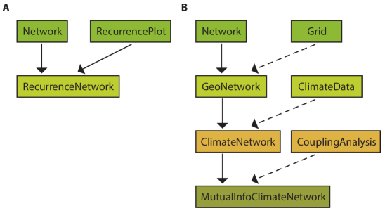
Figure 1: Examples for the software architecture of pyunicorn displayed as a Unified Modeling Language (UML) diagram of class relationships: ancestry of the (A) timeseries.RecurrenceNetwork (Sect. IV.1.2) and (B) climate.MutualInfoClimateNetwork classes (Sect. III.2). Inheritance (class B inherits from class A, solid arrows) and object composition relationships (class B contains class A, dashed arrows) are indicated.

pyunicorn is intended as an integrated container for a host of conceptionally related methods which have been developed and applied by the involved research groups for many years. Its aim is to establish a shared infrastructure for scientific data analysis by means of complex networks and non-linear time series analysis and it has greatly taken advantage from the backflow contributed by users all over the world. The code base has been fully open sourced under the BSD 3-Clause license.

With a focus on complex network methods, this software is a valuable complement to traditional non-linear time series analysis tools such as TISEAN (Hegger, Kantz, and Schreiber, 1999). Its main mode of operation is to import, generate and export complex networks from time series or fields thereof, and to compute appropriate measures on these networks in order to derive insights into the causal structure and dynamical regimes of underlying processes. While pyunicorn’s development has mostly accompanied advances in climatology and paleoclimatology, the generality of the network approach and its implementation of extensions to standard complex networks like spatio-temporal networks, node weighted measures, coupled functional networks and recurrence networks render the software widely applicable in numerous fields, e.g. medicine, neuroscience, sociology, economics and finance. Great care has been taken in linking to relevant publications from the method descriptions contained in the code and API documentation (Sup, ).

As the name suggests, the language chosen for the implementation is Python, which is very well established in scientific computing (Oliphant, 2007; Millman and Aivazis, 2011). Due to the multiplicity of useful combinations of methods, there are no executables in pyunicorn, but the library is intended to be used by small Python scripts. Its object-oriented software architecture allows for clean and flexible code representing the logical interrelationships and dependencies between the various concepts and methods (Sect. I.2). For example, the class RecurrenceNetwork (Sect. IV.1.2) inherits from both the Network (Sect. II.1) and RecurrencePlot classes (Sect. IV.1.1), thus reflecting the mathematical definition and historical development of recurrence network analysis (Fig. 1A). Following a similar reasoning behind the implementation of a class hierarchy, the climate network class MutualInfoClimateNetwork (Sect. III.2) inherits from the Network class via the intermediate parent classes GeoNetwork (Sect. II.2) and ClimateNetwork (Sect. III.2), additionally including several object composition relationships on the way (Fig. 1B).

While ensuring accessibility and maintainability among scientists in the disciplines mentioned above, this design facilitates fully flexible use of the package, from interactive local sessions in IPython (Pérez and Granger, 2007) to massively parallel computations on cluster architectures. For several years now, pyunicorn has been successfully deployed on Linux, Mac OS X and Windows systems as well as UNIX high performance clusters.

Besides Numpy (van der Walt, Colbert, and Varoquaux, 2011) and Scipy (Jones et al., 2001), which are among the most widely spread libraries for scientific computing in Python, pyunicorn’s only hard dependency is the igraph network analysis package (Csárdi and Nepusz, 2006). pyunicorn does not possess its own graphical interface, but where visual output is meaningful, helper methods exist for plotting with matplotlib (Hunter, 2007), which is especially convenient in IPython. Interfaces to tools for advanced network visualization focussing on spatial networks (Nocke et al., 2015) such as CGV (Tominski, Abello, and Schumann, 2009; Tominski, Donges, and Nocke, 2011) are provided via pyunicorn’s input-output capabilities. Commented examples for typical use cases are provided by the extensive software documentation.

I.2 Software structure

Table 1: Structure of the pyunicorn software package listing the most important classes belonging to each submodule (selection for brevity).

core	funcnet	climate	timeseries	utils
(Sect. II)	(Sect. III)	(Sects. III.2, III.3)	(Sects. IV, V)	(Sect. I)
Network	CouplingAnalysis	ClimateNetwork	RecurrencePlot	mpi
GeoNetwork	CouplingAnalysisPurePython	CoupledClimateNetwork	CrossRecurrencePlot	navigator
InteractingNetworks		TsonisClimateNetwork	JointRecurrencePlot
ResNetwork		SpearmanClimateNetwork	RecurrenceNetwork
Data		MutualInfoClimateNetwork	InterSystemRecurrenceNetwork
Grid		ClimateData	JointRecurrenceNetwork
			VisibilityGraph
			Surrogates

The pyunicorn library is fully object-oriented and its inheritance and composition hierarchy reflects the relationships between the analysis methods in use (Fig. 1). It consists of five subpackages (Tab. 1):

core

This name space contains the basic building blocks for general network analysis and modeling and is accessible after calling import pyunicorn (Sect. II). The backbone Network class provides numerous standard and advanced complex network statistics, measures and generative models as well as import and export capabilities to GraphML, GML, NCOL, LGL, DOT, DIMACS and other formats. Grid and GeoNetwork extend these functionalities with respect to spatio-temporally embedded networks, which can be imported from and exported to ASCII and NetCDF files via the Data class. InteractingNetworks provides advanced methods designed for networks of networks (or multiplex networks), while ResNetwork specializes in power grids transporting electric currents and related infrastructure networks.

funcnet

Advanced tools for construction and analysis of general (non-climate) functional networks will be accommodated here. So far, CouplingAnalysis calculates cross-correlation, mutual information, mutual sorting information and their respective surrogates for large arrays of scalar time series (Sect. III).

climate

Building on top of GeoNetwork and Data, the ClimateNetwork class and its children facilitate the construction and analysis of functional networks representing the statistical interdependency structure within a field of time series, based on similarity measures such as lagged linear Pearson or Spearman correlation and mutual information (Sect. III.2). CoupledClimateNetwork extends this capability to the study of interrelationships between two distinct fields of observables (Sect. III.3).

timeseries

This subpackage provides various tools for the analysis of non-linear dynamical systems and uni- and multivariate time series (Sect. IV). Apart from visibility graphs with time-directed measures (VisibilityGraph class), the focus lies on recurrence-based methods derived from the RecurrencePlot class. These include single, joint and cross-recurrence plots as well as standard, joint and inter-system recurrence networks, supporting time-delay embedding and several phase space metrics and are equipped with common measures of recurrence quantification analysis. Surrogates allow testing for the statistical significance of similarity measures by generating surrogate data sets under miscellaneous constraints from observable time series (Sect. V).

utils

Currently this includes MPI parallelization support and an experimental interactive network navigator.

I.3 General computational issues

Most network measures are defined as aggregates of local information obtained from topology, node weights and link attributes. Since pyunicorn internally represents networks as sparse adjacency matrices, it can handle large data sets. Until streaming algorithms are implemented for all measures, the available amount of working memory (RAM) limits the size of networks which can be processed. Presently, many advanced methods are defined only for undirected networks. As sensible generalizations and applications come up, they are gradually incorporated into the code base.

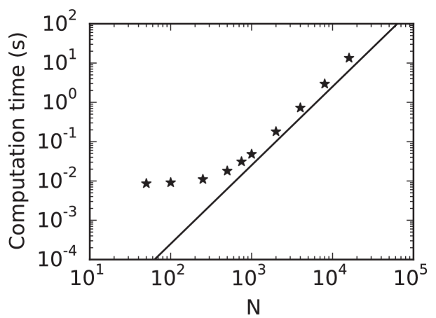
Figure 2: Dependence of computation time for constructing recurrence networks (represented by RecurrenceNetwork objects) of varying size $N$ constructed from state vectors randomly drawn from the Lorenz attractor (see Fig. 15) on a dual-core Intel Core i5 CPU with 2.4 GHz running Mac OS X (star symbols). For larger $N$, computation time is proportional to $N^{2}$ (solid line) as expected for the straightforward algorithm implemented for calculating the $N\times N$ recurrence matrix $\mathbf{R}$. Note that fast neighbor search algorithms, currently not implemented in pyunicorn, can reduce the number of required computations to $\mathcal{O}(N\log N)$ or even $\mathcal{O}(N)$ under certain conditions (Hegger, Kantz, and Schreiber, 1999).

As is usually the case with Python libraries, pyunicorn is designed to provide simple interfaces and clear architecture, while delegating the heavy lifting to specialized tools for performance. Basic network measures and generative models are inherited from igraph. Wherever possible, numerically intensive computations are expressed as combinations of highly optimized linear algebra methods from Numpy and Scipy, and otherwise implemented in embedded Cython (Behnel et al., 2011) code. Thus all costly computations are performed in compiled C, C++ or FORTRAN code. Parallelization is mostly not implemented on the algorithm level, but can be achieved using the built-in MPI helper for repetitive tasks, e.g. computing measures on recurrence networks for different time windows of an observable. As the required RAM size is mostly dependent on the volume of data to be analyzed, a modern laptop processor with a single core suffices to perform most of the computations described later on for currently typical data sets in a matter of seconds to an hour. As an example, the recurrence network displayed in Fig. 15 takes approximately 0.03 seconds to compute on a dual-core Intel Core i5 CPU with 2.4 GHz running Mac OS X. For illustration, a more systematic study of the performance of recurrence network construction, a common task of using pyunicorn, is displayed in Fig. 2. GPU computations are currently not supported.

II Complex network analysis

pyunicorn provides methods for analyzing and modeling various types of complex networks, including general networks (Sect. II.1), spatial networks (Sect. II.2), networks of interacting networks (Sect. II.3) and node-weighted networks (Sect. II.4). In the following, the corresponding classes and methods are described together with a brief introduction of the underlying theory. Selected use cases illustrate the associated functionality of pyunicorn.

II.1 General complex networks

The class Network in the submodule core serves as a parent to all other network-related classes in pyunicorn (see, e.g. Fig. 1) and represents general undirected and directed networks or graphs $G=(V,E)$ consisting of a set of nodes $V=\{1,\dots,N\}$ and a set of (directed) links $E\subseteq V\times V$ without dublicates. Networks of this type can be described by an adjacency matrix $\mathbf{A}$ with elements

$$A_{pq}=\begin{cases}1&(p,q)\in E\\ 0&\text{otherwise}.\end{cases}$$ (1)

Hence, $A_{pq}=1$ iff nodes $p$ and $q$ are connected by a (directed) link and $A_{pq}=0$ iff they are unconnected. In pyunicorn, instances of the Network class can be initialized using such dense adjacency matrices, but also based on sparse matrices or link lists. Link and node weights (see Sect. II.4) can be represented by link and node attributes and are accessible through the Network.set_link_attribute and Network.set_node_attribute methods, respectively.

Many standard complex network measures, network models and algorithms are supported, e.g. degree, closeness and shortest-path betweenness centralities, clustering coefficients and transitivity, community detection algorithms and network models such as Erdős-Rényi, Barabasi-Albert or configuration model random networks (Cohen and Havlin, 2010; Newman, 2010). Several of these measures provided by pyunicorn can take into account directed links and link weights (directed and weighted networks) if this information is present. However, the remainder of this article focusses on undirected networks, reflecting the current state of the pyunicorn implementation.

Moreover, a number of less common network statistics such as Newman’s (Newman, 2005) or Arenas’ (Arenas et al., 2003) random walk betweenness can be computed. Reading and saving network data from and to many common data formats such as GraphML (Brandes et al., 2002) is possible for storage and information exchange with other software for network analysis and visualization (Nocke et al., 2015) such as networkx (Schult and Swart, 2008) or gephi (Bastian, Heymann, and Jacomy, 2009).

II.2 Spatially embedded networks

Many, if not most, complex networks of interest are spatially embedded (Barthélemy, 2011). Consider, for example, social networks, infrastructure networks such as the internet, road and other transportation networks (Fig. 3) or functional networks in neuroscience and climatology (Fig. 8). pyunicorn includes measures and models specifically designed for spatially embedded networks (or simply spatial networks) via the GeoNetwork class that inherits from the Network class (Fig. 1B). Characteristics of the nodes’ spatial embedding, such as all longitudinal and latitudinal coordinates, are stored in the Grid class. In particular, this class then provides methods for computing and evaluating spatial distances between all pairs of nodes via the methods Grid.angular_distance, Grid.euclidean_distance and Grid.geometric_distance_distribution. Additionally, functionality for loading and saving the grid from and to common file formats such as ASCII is provided.

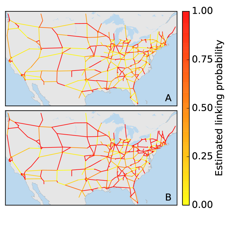
Figure 3: Effects of spatial embedding of nodes on network structure: (A) Probability for links in the US interstate network to be also present under the application of GeoModel1 computed over an ensemble of $100$ surrogate networks using GeoNetwork.randomly_rewire_geomodel_I. (B) The same under the application of GeoModel2 provided by GeoNetwork.randomly_rewire_geomodel_II.

II.2.1 Measures and models for spatial networks

Measurements on the network’s spatial embedding are performed by using the class GeoNetwork which is initialized with an existing instance of the Grid class (Fig. 1B). Generally, all standard network measures, like the degree or clustering coefficient, can be computed in an area-weighted variant taking into account the network’s spatial embedding and, hence, avoiding biases caused by the potentially widely different surface areas or volumes that nodes may represent (see Sec. IID for details). In addition, the distribution of the links’ spatial lengths are evaluated using the method GeoNetwork.link_distance_distribution. For each node in the network the lengths of its emerging links can be assessed via the methods GeoNetwork.average_link_distance, GeoNetwork.total_link_distance and GeoNetwork.max_link_distance which all give a notion of the spatial distance between a specific node and its neighbors. In the application to climate sciences, where links in the network typically represent interdependencies of statistical significance between climate observables taken at different locations on the Earth’s surface, the above mentioned measures are of crucial importance when investigating the presence of long-ranging teleconnections (Donges et al., 2009b; Tsonis and Roebber, 2004; Tsonis, Swanson, and Wang, 2008) in the climate network (Sect. III.2).

In addition to the evaluation of a spatially embedded network’s topological structure, the GeoNetwork class also provides random network models to construct spatially embedded networks under the same spatial constraints, i.e. with the same spatial distribution of nodes, as the network under study. These spatial network surrogates allow to assess to what degree certain properties of an observed network are consistent with those expected from a structural null model that is encoded in the construction rules for the network surrogates. In particular, the method GeoNetwork.set_random_links_by_distance constructs a random network in which the probability for the presence of a link between two nodes decays exponentially with the geographical distance between them. Furthermore, three different GeoModels are implemented in pyunicorn which construct random network surrogates of a given network by iteratively rewiring its links under different conditions: (i) GeoModel1 (GeoNetwork.randomly_rewire_geomodel_I) creates a random network with the same link-length distribution and link density as the one represented by the respective instance of GeoNetwork. (ii) GeoModel2 (GeoNetwork.randomly_rewire_geomodel_II) additionally preserves the local link-length distribution and degree of each node, and (iii) GeoModel3 (GeoNetwork.randomly_rewire_geomodel_III) additionally sustains the degree-degree correlations (or assortativity) of the original network (Wiedermann et al., 2015a).

II.2.2 Use case: US interstate network

We illustrate the application of these random spatial network models by constructing $100$ surrogate networks of the US interstate network (Gastner and Newman, 2006) utilizing GeoModel1 and GeoModel2, respectively. One way to quantify how well the network under study is represented by each of the two models is to compute the probability that each of its links is also present in the ensemble of random surrogates (Fig. 3). We find that GeoModel1 already reproduces well many of the original links in the US interstate network (Fig. 3A), implying that its structure is already well determined by its global link length distribution. Additionally preserving the local link length distributions and degree sequence improves the results further: most links of the original network are present in the surrogate networks with high probability (Fig. 3B).

II.3 Networks of interacting networks

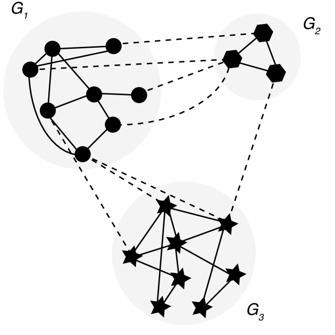
Figure 4: A network of interacting networks consisting of three subnetworks $G_{i}$ that can be represented and analyzed using the class core.InteractingNetworks. Nodes are represented by geometric symbols, while internal and cross-links are indicated by solid and dashed lines, respectively.

The structure of many complex systems can be described as a network of interacting or interdependent networks (Donges et al., 2011a; Wiedermann et al., 2013), e.g. the densely entangled infrastructures for communication and energy distribution (Buldyrev et al., 2010; Gao et al., 2012). Constituting a specific but important subclass of multiplex or multilayer networks (Boccaletti et al., 2014), these networks of networks can be represented by decomposing a network $G=(V,E)$ into a collection of $M$ subnetworks $G_{i}=(V_{i},E_{ii})$ (Fig. 4). Here, $V_{i}$ denote the disjunct sets of nodes corresponding to each subnetwork and the internal links sets $E_{ii}$ contain information on the connections within a subnetwork such that $\bigcup_{i=1}^{M}V_{i}=V$. Additionally, disjunct sets of cross-links $E_{ij}$ connect nodes in different subnetworks with $\bigcup_{i,j=1}^{M}E_{ij}=E$. Alternatively, a network of networks (multiplex network) of this type can be represented by a standard adjacency matrix $\mathbf{A}$ with block structure (Donges et al., 2011a). Depending on the problem at hand, the decomposition into subnetworks can be given a priori, as in the example of interdependent communication and electricity grids, or may be obtained from solutions of a community detection algorithm applied to a complex network of interest (Girvan and Newman, 2002; Newman, 2006; Fortunato, 2010).

II.3.1 Measures and models for networks of networks

The InteractingNetworks class in the submodule core provides a rich collection of network measures and models specifically designed for investigating the structure of networks of networks (Donges et al., 2011a; Wiedermann et al., 2013). Relevant examples include the cross-link density of connections between different subnetworks (InteractingNetworks.cross_link_density)

$$\rho_{ij}=\frac{|E_{ij}|}{|V_{i}||V_{j}|},$$ (2)

the cross-degree or number of neighbors of node $v\in V_{i}$ in a different subnetwork $G_{j}$ (InteractingNetworks.cross_degree)

$$k_{v}^{ij}=\sum_{q\in V_{j}}A_{vq},$$ (3)

or the cross-shortest path betweenness (InteractingNetworks.cross_betweenness) defined for all nodes $w\in V$:

$$b_{w}^{ij}=\sum_{p\in V_{i},q\in V_{j};p,q\neq w}\frac{\sigma_{pq}(w)}{\sigma_{pq}}$$ (4)

quantifying the importance of nodes for mediating interactions between different subnetworks, where $\sigma_{pq}$ denotes the total number of shortest paths from $p\in V_{i}$ to $q\in V_{j}$ and $\sigma_{pq}(w)$ counts the number of shortest paths between $p$ and $q$ that include $w$. The InteractingNetworks class also contains node-weighted versions of most of the provided statistical measures (see Sect. II.4).

Surrogate models of interacting networks allow the researcher to assess the degree of organization in the cross-connectivity between subnetworks and its effects on other network properties of interest such as (cross-) clustering and (cross-) transitivity or shortest-path based measures such as (cross-) average path length or (cross-) betweenness (Donges et al., 2011a). Specifically, pyunicorn currently supports two types of interacting network models that conserve (i) the number of cross-links or the cross-link density between a pair of subnetworks (InteractingNetworks.RandomlySetCrossLinks), analogously to the Erdős-Rényi model (Erdős and Rényi, 1959) for general complex networks, and (ii) the cross-degree sequences between a pair of subnetworks (InteractingNetworks.RandomlyRewireCrossLinks), corresponding to the configuration model for standard networks (Newman, 2003).

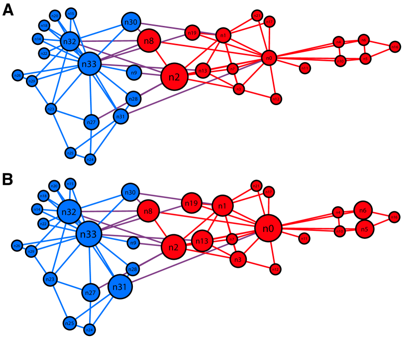
Figure 5: Visualization of the Zachary karate club network with node colors indicating the two groups emerging after fission that were lead by individuals 0 (subnetwork $G_{1}$, red nodes) and 33 (subnetwork $G_{2}$, blue nodes), respectively (note that the original node numbering of Zachary (1977) can be obtained by adding 1 to these indices). Node size is scaled according to the (A) cross-degree and (B) cross-betweenness (log-scale) measures of interacting networks analysis. Internal links are colored in red and blue, while cross-links are displayed in violet.

In the context of time series analysis, the interacting network representation has been applied for studying the structure of statistical interrelationships between different climatological fields with coupled climate networks (Donges et al., 2011a; Wiedermann et al., 2015b) (Sect. III.3) as well as for detecting the direction of coupling between complex dynamical systems using inter-system recurrence networks (Feldhoff et al., 2012) (Sect. IV.1).

II.3.2 Use case: Zachary karate club network

For illustrating interacting networks analysis based on a simple and commonly studied example, we choose the classical Zachary karate club social network that describes friendship relationships between 34 members of a karate club at a US university (Zachary, 1977). During the course of the study, a disagreement developed between some of the members and the club split up into two parts. Here, we represent the groups after fission by two subnetworks $G_{1}$ (lead by individual 0) and $G_{2}$ (lead by individual 33) with internal and cross-links set according to the friendship ties revealed in the original study (Fig. 5). The groups emerging after fission are clearly reflected in the social network structure as was also found using various community detection algorithms (Girvan and Newman, 2002; Newman, 2006). The cross-link density $\rho_{12}\approx 0.04$ is significantly smaller than the internal link densities $\rho_{11}\approx 0.26$ and $\rho_{22}\approx 0.24$, underlining the conceptual similarities between interacting network characteristics such as cross-link densities or cross-degree sequences and measures of modularity used for community detection (Newman, 2006).

Furthermore, studying local interacting network measures yields insights into the roles of nodes with respect to interactions between the two groups. For example, nodes on the interface between both groups such as individuals 2, 8 and 30 tend to have large cross-degree and cross-betweenness values compared to other nodes on the groups’ peripheries, because they serve as important connectors between the groups (Fig. 5). Focussing on the two group leaders, it is interesting to note that individual 0 (the instructor) has a low cross-degree (just one cross-link to $G_{2}$, $k_{0}^{1\,2}=1$) compared to individual 33 (the administrator, $k_{33}^{2\,1}=3$), while both leaders have comparable first and second largest values of cross-betweenness, $b_{0}^{1\,2}\approx 148$ and $b_{33}^{1\,2}\approx 94$, respectively. This observation indicates that cross-betweenness is a more reliable indicator for leadership with respect to the groups’ interaction structure in this case.

II.4 Node-weighted networks and node-splitting invariance

The nodes of many real-world networks, e.g. firms, countries, grid cells, brain regions etc., are of heterogeneous size, represent different shares of an underlying complex system, or are of different prior relevance to the research question at hand. As a specific example, in climate networks on regular latitude-longitude grids (see below and Fig. 6), nodes in polar regions represent a significantly smaller fraction of the Earth’s surface than do nodes in the tropics. If this heterogeneity can be expressed in a vector of node weights $w_{v}\geq 0$ with $v\in V$, a node-weighted network analysis seems appropriate. Because many complex systems allow for network representations of different granularity, the results of such a node-weighted network analysis should be consistent across scales (Heitzig et al., 2012). pyunicorn provides node-weighted variants of most standard and many non-standard measures for networks (Network class) as well as interacting networks (InteractingNetworks class).

II.4.1 Measures for node-weighted networks

The theory of node-splitting invariant (n.s.i.) network measures (Heitzig et al., 2012; Rheinwalt et al., 2012; Radebach et al., 2013; Wiedermann et al., 2013; Molkenthin et al., 2014a; Zemp et al., 2014a, b; Feldhoff et al., 2015; Lange et al., 2015; Rheinwalt et al., 2015) has derived variants of many classical network measures that take into account node weights in a consistent way. For example, the n.s.i. adjacency matrix $A^{+}_{pq}$, degree $k^{\ast}_{v}$, local and global clustering coefficients $\mathcal{C}^{\ast}_{v},\mathcal{C}^{\ast}$ are defined as

$$A^{+}_{pq} =A_{pq}+\delta_{pq}, \mathcal{C}^{\ast}_{v} =\frac{\sum_{p,q\in V}A^{+}_{vp}w_{p}A^{+}_{pq}w_{q}A^{+}_{qv}}{(k^{\ast}_{v})^{2}},$$

$$k^{\ast}_{v} =\sum_{p\in V}A^{+}_{vp}w_{p}, \mathcal{C}^{\ast} =\sum_{v\in V}w_{v}\mathcal{C}^{\ast}_{v}/\sum_{v\in V}w_{v}.$$ (5)

In contrast to their unweighted counterparts, these and all other n.s.i. measures have the following consistency property: When a node $v$ and its weight $w_{v}$ are split into two interlinked nodes $v^{\prime},v^{\prime\prime}$ with weights $w_{v^{\prime}}+w_{v^{\prime\prime}}=w_{v}$ that are connected to the same nodes as $v$ was, then all n.s.i. measures of nodes other than $v$, $v^{\prime}$, and $v^{\prime\prime}$ remain unchanged (e.g. the n.s.i. clustering coefficient of some neighbour $p$ of $v$ remains unchanged while the ordinary clustering coefficient of $p$ would increase). This scale consistency comes at the price that in the special case where all weights are equal to unity, $w_{v}\equiv 1$, n.s.i. measures do not simply reduce to their unweighted counterparts but return slightly different values. For this reason, there exist also corrected n.s.i. measures that additionally take into account an overall typical weight $\omega\geq 0$ and have the property that in the special case where all node weights equal $\omega$, the corrected n.s.i. measure equals its unweighted counterpart (Heitzig et al., 2012) . For example, the corrected n.s.i. degree $k^{\ast\omega}_{v}$ and local clustering coefficient $\mathcal{C}^{\ast\omega}_{v}$ are

$$k^{\ast\omega}_{v} =\textstyle\frac{k^{\ast}_{v}}{\omega}-1, \mathcal{C}^{\ast\omega}_{v} =\textstyle\frac{\sum_{p,q\in V}A^{+}_{vp}w_{p}A^{+}_{pq}w_{q}A^{+}_{qv}-3k^{\ast\omega}_{v}-1}{k^{\ast\omega}_{v}(k^{\ast\omega}_{v}-1)}.$$ (6)

In pyunicorn, n.s.i. measures are available in the Network and InteractingNetworks classes (method prefix nsi_), e.g.:

    nsi_arenas_betweenness,
    nsi_average_neighbors_degree,
    nsi_average_path_length,
    nsi_betweenness,
    nsi_closeness,
    nsi_degree.

Their syntax is the same as that of their unweighted counterparts, and some have an additional optional keyword parameter typical_weight via which the corrected n.s.i. measures can be requested. To use these methods, one has to provide node weights before, either manually via the Network property node_weights, the keyword parameter node_weights of the class constructor, or automatically via the keyword parameter node_weight_type of the constructor of the derived class GeoNetwork.

II.4.2 Use case: spatial network structures in polar region

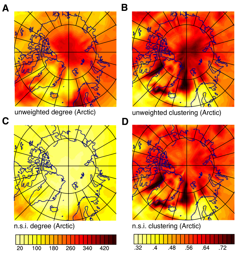
Figure 6: Comparison of unweighted and weighted (n.s.i.) versions of degree (A,C) and local clustering coefficient (B,D) in the northern polar region (Lambert equal area projection) of a global climate network representing correlations in temperature dynamics. The high values at the pole in (A,B) turn out to be an artifact of the increasing grid density toward the pole, as demonstrated by (C,D). Reproduced with permission from Eur. Phys. J. B 85, 38 (2012) Heitzig et al. (2012). Copyright 2012 European Physical Society and Springer-Verlag.

Figure 6 presents an application of n.s.i. degree and local clustering coefficient to the functional climate network of surface air temperature dynamics in the northern polar region (Heitzig et al., 2012). A ClimateNetwork object net was generated as described in Sect. III.2, with nodes placed on a regular latitude-longitude grid on the Earth’s surface. To reflect that grid’s varying node density depending on latitude, the node weights were set to the cosine of latitude by using the ClimateNetwork constructor’s keyword parameter node_weight_type="surface" (inherited from GeoNetwork, see Fig. 1B). Then all nodes’ n.s.i. degree and local clustering coefficient were computed via

    kstarvector = net.nsi_degree()
    Cstarvector = net.nsi_local_clustering()

and plotted using the package matplotlib. When comparing the resulting node-weighted measures (Fig. 6C,D) to the unweighted degree and local clustering coefficient (Fig. 6A,B), one realizes that the latter measures’ high values around the pole (dark spots) are actually artifacts of the relatively higher node density, an effect that is compensated for in the n.s.i. measures.

III Functional networks: construction and analysis

Functional networks provide a powerful generalization of standard methods of bi- and multivariate time series analysis by allowing to study the dynamical relationships between subsystems of a high-dimensional complex system based on spatio-temporal data and using the tools of network theory. pyunicorn provides classes for the construction and analysis of functional networks representing the statistical interdependency structure within and between sets (fields) of time series using various similarity measures such as lagged Pearson correlation and mutual information (Sect. III.1). Building on these similarity measures, climate networks allow for the analysis of single fields of climatological time series, e.g. surface air temperature observed on a grid covering the Earth’s surface (Sect. III.2). Moreover, coupled climate networks focus on studying the interrelationships between two or more fields of climatological time series, e.g. sets of time series capturing sea surface temperature and atmospheric geopotential height variability (Sect. III.3). Functional network analysis is illustrated drawing upon several examples from climatology, including the detection of spatio-temporal regime shifts in the atmosphere and ocean. While pyunicorn provides some functionality specific to climate data (such as the climate.ClimateData class), the methods for general functional network analysis can also be applied to other sources of time series such as general fluid dynamical and pattern formation systems (Molkenthin et al., 2014b), neuroscience (e.g. functional magnetic resonance imaging, fMRI, and electroencephalogram [EEG] data; Bullmore and Sporns (2009)) or finance (e.g. stock market indices; Huang, Zhuang, and Yao (2009)).

III.1 Coupling analysis

The timeseries.CouplingAnalysis class provides methods to estimate matrices of (optionally lagged) statistical similarities $\mathbf{S}$ between time series including on the linear Pearson product-moment correlation and measures from information theory such as mutual information and extensions thereof. These matrices can be thresholded to obtain directed or undirected adjacency matrices for further network analysis with pyunicorn, e.g. as input to the climate.ClimateNetwork (Sect. III.2) and climate.CoupledClimateNetwork (Sect. III.3) classes. The similarity values can also be used in link-weighted network measures such as those provided by the Network class.

III.1.1 Similarity measures for time series

While standard measures such as the classical linear Pearson product-moment correlation are only briefly discussed, this section focusses on more innovative measures based on information theory that are provided by the CouplingAnalysis class. The latter include bivariate mutual information as well as its multivariate extensions allowing to reduce the effects of common drivers or indirect couplings (Fig. 7A) on estimates of information transfer between two processes $X,\,Y$ ($X$ and $Y$ represent time series at nodes $p$ and $q$, respectively).

All methods share the parameters tau_max, the maximum time lag, and lag_mode, which can be set to ’all’ to obtain a 3-dimensional Numpy array of shape $(\texttt{N},\,\texttt{N},\,\texttt{tau\_max + 1})$ containing lagged similarities between all pairs of nodes, or to ’max’ to return two $(\texttt{N},\,\texttt{N})$ Numpy arrays indicating the lag positions and values of the absolute similarity maxima.

Lagged cross-correlation

The lagged Pearson product-moment correlation coefficient (CC) of two zero-mean time series variables $X,\,Y$, implemented in CouplingAnalysis.cross_correlation, is given by

$$\rho_{XY}(\tau)=\frac{\left<X_{t-\tau},Y_{t}\right>}{\sigma_{X}\sigma_{Y}},$$ (7)

which depends on the covariance $\left<X_{t-\tau},Y_{t}\right>$ and standard deviations $\sigma_{X},\,\sigma_{Y}$. Lags $\tau>0$ correspond to the linear association of past values of $X$ with $Y$, and vice versa for $\tau<0$. In analogy, the auto-correlation is defined as $\rho_{YY}(\tau)$ for $\tau>0$. The choice lag_mode=’max’ returns the value and lag at the absolute maximum for each ordered pair $(i,j)$, which can be positive or negative. CC is computed using the standard sample covariance estimator. It can be estimated for comparably small sample sizes. However, by definition, it does not allow to quantify nonlinear associations between time series and can produce misleading results in the presence of strongly nonlinear relationships.

Lagged mutual information

Information theory (Cover and Thomas, 2006) provides a genuine framework to capture also nonlinear associations. While Shannon entropy (Shannon, 1948) is a measure of the uncertainty about outcomes of one process, mutual information (MI) is a measure of its reduction if another process is known. The Shannon-type MI can be expressed as

$$I(X;Y) =H(Y)-H(Y|X)=H(X)-H(X|Y),$$ (8)

i.e. as the difference between the uncertainty in $Y$ and the remaining uncertainty if $X$ is already known (and vice versa). MI is symmetric in its arguments, non-negative and zero iff $X$ and $Y$ are statistically independent. The lagged cross-MI for two time series, implemented in CouplingAnalysis.mutual_information, is given by

$$I^{\rm MI}_{XY}(\tau)=I(X_{t-\tau};Y_{t}).$$ (9)

For $\tau>0$, one measures the information in the past of $X$ that is contained in $Y$, and vice versa for $\tau<0$. Correspondingly, the auto-MI is defined as $I(Y_{t-\tau};Y_{t})$ for $\tau>0$.

Three different estimators are provided reflecting different trade-offs between number of samples required, bias and variance of the estimator, and computational requirements:

• estimator=’binning’: A very simple method is to quantize or partition the observation space into a set of bins (parameter bins). Here, we use equi-quantile bins where the bin intervals are chosen such that the marginal distributions are uniform (Paluš, 1996). While this estimator is consistent for infinite sample size, for common sample sizes of the order $10^{3}$, many bins are not populated sufficiently resulting in heavily biased values of MI (Hlaváčková-Schindler et al., 2007). For example, for independent time series the estimated MI values do not center around zero.

• estimator=’knn’: A more advanced estimator for continuously valued variables, recommended here, is based on nearest-neighbor statistics (Kraskov, Stögbauer, and Grassberger, 2004). This estimator is discussed in its conditional form below.

• estimator=’gauss’: If only the linear part of an association is desired, assuming a bivariate Gaussian distribution, the MI is simply given by

  $$I^{\rm Gauss}_{XY}(\tau)=-\tfrac{1}{2}\ln\left(1-\rho_{XY}(\tau)^{2}\right),$$ (10)

  where $\rho_{XY}(\tau)$ is again the Pearson correlation coefficient.

Lagged information transfer

While lagged MI can be used to quantify whether information in $Y$ has already been present in the past of $X$, this information could also stem from the common past of both processes and, therefore, is not necessarily a sign of a transfer of unique information from $X$ to $Y$. A first step toward a notion of directionality (the more demanding causality problem is discussed at the end of this section) is to assess a bivariate notion of information transfer between two time series (Runge et al., 2012a; Hlinka et al., 2013) in order to exclude this common past. Here, we consider two measures to achieve this goal, implemented in CouplingAnalysis.information_transfer. These are based on conditional mutual information (CMI) defined as

$$I(X;Y|Z) =H(Y|Z)-H(Y|X,Z)$$ (11)

which can be phrased as the mutual information between $X$ and $Y$ that is not contained in a third, possibly multivariate variable $Z$. CMI shares the properties of MI and is zero iff $X$ and $Y$ are independent conditionally on $Z$.

Following Runge et al. (2012a), the bivariate information transfer to Y (ITY), obtainable via the parameter cond_mode=’ity’, is defined as

$$I_{X\to Y}^{\rm ITY}(\tau) =I(X_{t-\tau};Y_{t}|Y_{t-1},\ldots,Y_{t-p}).$$ (12)

It excludes the past of the ‘driven variable’ $Y$ up to a maximum lag $p$ (parameter past). ITY can be seen as a lag-specific transfer entropy (Schreiber, 2000). A more rigorous way to exclude commonly shared past is to additionally condition out the past of the ‘driver’ variable $X$. The bivariate momentary information transfer (MIT), called via cond_mode=’mit’, can be defined as

$$I^{\rm MIT}_{X{\to}Y}(\tau)=$$

$$I(X_{t-\tau};Y_{t}|Y_{t-1},\ldots,Y_{t-p},X_{t-\tau-1},\ldots,X_{t-\tau-p})$$ (13)

The attribute momentary (Pompe and Runge, 2011) is used because MIT measures the information of the “moment” $t-\tau$ in $X$ that is transferred to $Y_{t}$. MIT can also be interpreted as a measure of causal strength as discussed in Runge et al. (2012a), where the multivariate versions of ITY and MIT are defined. On the downside, it is higher-dimensional resulting in a larger bias for the nearest-neighbor estimator.

Two estimators are available:

• estimator=’gauss’: Like in Eq. (10), the CMI for multivariate Gaussians can be expressed in terms of the partial correlation, where the Pearson correlation $\rho_{XY}$ is replaced by $\rho_{XY|Z}$.

• estimator=’knn’: A nearest-neighbor CMI estimator has been developed by Frenzel and Pompe (2007). This estimator is computed by choosing a parameter $k$ (knn) as the number of neighbors in the joint space of $(X,\,Y,\,Z)$ around a sample at time $t$. The maximum-norm distance to the $k$-th nearest neighbor then defines a hypercube of length $2\epsilon_{t}$ for each joint sample. Then the numbers of points $k_{z,t}$, $k_{xz,t}$ and $k_{yz,t}$ in the subspaces with distance less than $\epsilon_{t}$ are counted, and the CMI is estimated as

  $$\widehat{I}(X;Y|Z)=\psi(k)+\frac{1}{T}\sum_{t=1}^{T}\left[\psi(k_{z,t})-\psi(k_{xz,t})-\psi(k_{yz,t})\right],$$ (14)

  where $\psi$ is the Digamma function and $T$ is the number of samples. Smaller values of $k$ result in smaller cubes and, since as assumed in the estimator’s derivation, the density is approximately constant inside these, the estimator has a low bias. Conversely, for large $k$ the bias is stronger, but the variance is smaller. Note, however, that for independent processes the bias is approximately zero, i.e. $\widehat{I}(X;Y|Z)\approx 0$, and large $k$ are therefore better suited for (conditional) independence tests, e.g. on whether a link exists between two time series.

III.1.2 Use case: coupled stochastic processes

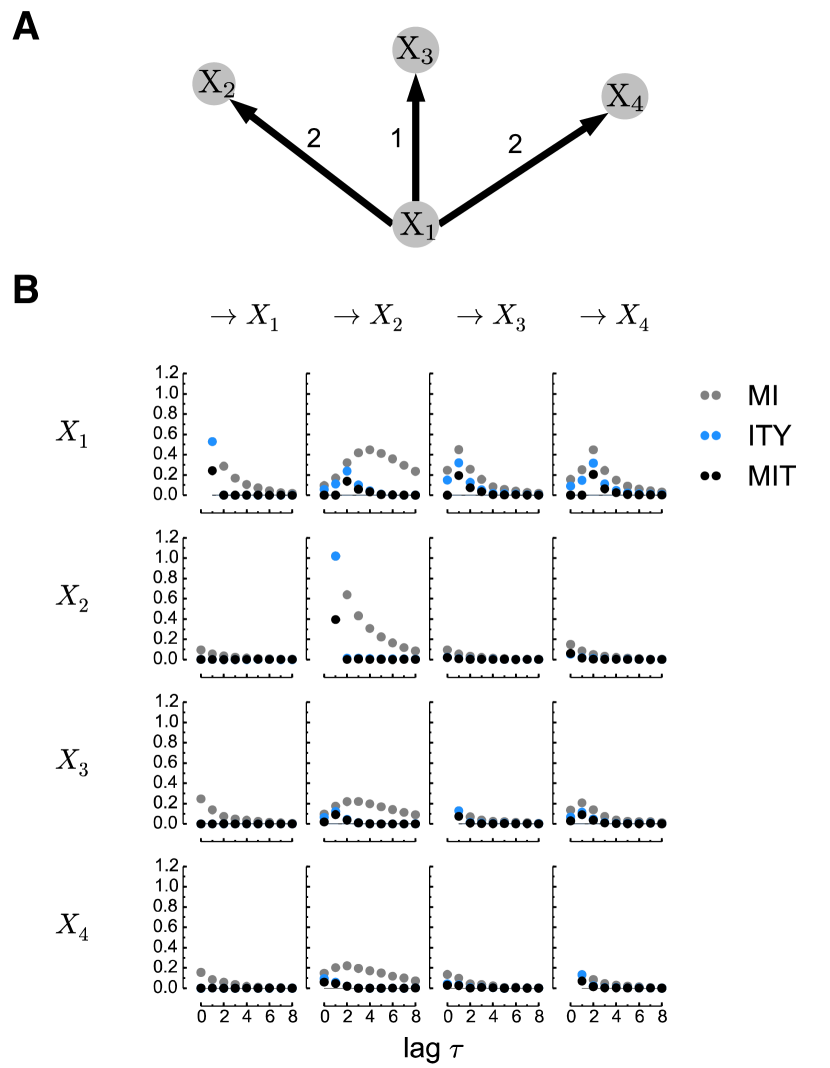
Figure 7: (A) Process graph and (B) matrix of lag functions for similarity measures MI, ITY, and MIT (the latter two with past-history parameter $p=1$) for a realization of example process (Eq. (III.1.2)). All methods implemented in CouplingAnalysis have a parameter lag_mode, which can be set to ’all’ to return all lagged similarities between all pairs of nodes (shape $(\texttt{N},\,\texttt{N},\,\texttt{tau\_max + 1})$, or to ’max’ to return two $(\texttt{N},\,\texttt{N})$-matrices of the value at the absolute maximum of each panel and the corresponding lags. Note that this results in an asymmetric matrix which can be symmetrized by taking the maximum of each pair $(i,j)$ and $(j,i)$ with the method CouplingAnalysis.symmetrize_by_absmax.

Consider the following simple four dimensional process to illustrate the different measures (Fig. 7A):

$$X_{1}(t) =0.8X_{1}(t-1)+\eta_{1}(t)$$

$$X_{2}(t) =0.8X_{2}(t-1)+0.5X_{1}(t-2)+\eta_{2}(t)$$

$$X_{3}(t) =0.7X_{1}(t-1)+\eta_{3}(t)$$

$$X_{4}(t) =0.7X_{1}(t-2)+\eta_{4}(t)\,,$$ (15)

where $\eta_{i}$ are independent zero-mean and unit variance Gaussian innovations. Here $X_{1,2}$ are auto-correlated and $X_{1}$ drives $X_{2}$ at a lag of 2, $X_{3}$ at a lag of 1, and $X_{4}$ at a lag of 2. Figure 7B shows the lag functions for all pairs of variables. We illustrate in the following, how the different measures MI (similar to CC), ITY, and MIT can be used to reconstruct an adjacency matrix of a functional network. Regarding a directed link between $X_{1}$ and $X_{2}$, both directions $X_{1}\to X_{2}$ and $X_{2}\to X_{1}$ have non-zero MI values, making it hard to conclude on a direction. Further, the peak of the MI function in $X_{1}\to X_{2}$ is at lag $\tau=4$, even though the driving lag is only 2. The ambiguity in interpreting the value of MI is discussed in (Runge et al., 2012a) and the problem that coupling delays cannot be properly inferred with MI because the peak of the lag function is shifted for strong auto-correlations is analyzed in Runge, Petoukhov, and Kurths (2014). These shortcomings can be overcome with ITY and MIT. Both measures feature a much sharper peak at the correct lag $\tau=2$. The value of MIT is smaller because it also excludes the effect due to the auto-correlation of the driving variable.

Still, all these bivariate lagged measures show non-zero values even if NO physical coupling is present in Eq. (III.1.2), e.g. in the lower two rows in Fig. 7B from $X_{3}$ and $X_{4}$ to the other processes. These artifacts are due to indirect links and common drivers (Fig. 7A), e.g. $X_{1}$ driving $X_{3}$, and $X_{4}$ leading to a spurious peak at $X_{3}\to X_{4}$. MI and the bivariate versions of ITY and MIT discussed here are also not able to reliably identify the correct coupling lags when multiple lags are present.

III.1.3 Discussion and extensions

Generally, networks reconstructed from bivariate similarity measures can be used to study statistical properties of associations between time series, but cannot be interpreted in a causal context. Based purely on observational data, a notion of a causal network can be defined within the framework of time series graphs (Eichler, 2012; Runge et al., 2012b), which can be efficiently estimated by causal discovery algorithms in a linear framework with partial correlation (Runge, Petoukhov, and Kurths, 2014; Schleussner et al., 2014) or with non-parametric information-theoretic estimators as implemented in the causal algorithm proposed in Runge et al. (2012b). Based on these causal graphs, multivariate versions of ITY and MIT can be used to quantify the links’ strength at the correct causal lag (Runge et al., 2012a). These methods are available in the software package tigramite, which can be obtained from the website http://tocsy.pik-potsdam.de/tigramite.php as a complement to pyunicorn. Note, however, that reliable causal analyses, especially with information-theoretic estimators, require much more samples than classical bivariate analysis, which typically restricts their applicability to much smaller networks (Balasis et al., 2013). An alternative to classical path-based network measures is discussed in Runge et al. (2015); Runge (2015) and introduces quantifiers of information transfer through causal pathways.

III.2 Climate networks

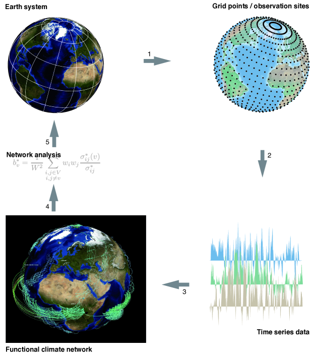
Figure 8: Workflow of functional network analysis illustrated for climate networks (modified from Donges (2012)). In step 1, a discretized time series representation $\{x_{v}(t)\}_{v=1}^{N}$ of the climatological field(s) of interest is chosen that is usually prescribed by the available gridded or station data. Step 2 includes time series preprocessing and the computation of similarity measures $S_{ij}$ for quantifying statistical interdependencies between pairs of climatological time series. In step 3, the construction of a climate network from the similarity matrix $\mathbf{S}$ typically involves some thresholding criterion (see Tominski, Donges, and Nocke (2011); Nocke et al. (2015) for details on the climate network shown here that was visualized using the software CGV (Tominski, Abello, and Schumann, 2009)). In step 4, the obtained climate network is investigated drawing on the tools of complex network theory. Finally, in step 5, the results of this analysis need to be interpreted in terms of the underlying dynamical Earth system.

As a typical application of functional networks, climate network analysis is a versatile approach for investigating climatological data and can be seen as a generalization and complementary method to classical techniques from multivariate statistics such as eigen analysis (e.g. empirical orthogonal function or maximum covariance analysis) (Donges et al., 2015a). It has been already successfully used in a wide variety of applications, ranging from the complex structure of teleconnections in the climate system (Tsonis and Roebber, 2004; Tsonis, Swanson, and Wang, 2008; Donges et al., 2009a), including backbones and bottlenecks (Donges et al., 2009b; Runge et al., 2015), to dynamics and predictability of the El Niño-Southern Oscillation (ENSO) (Radebach et al., 2013; Ludescher et al., 2013, 2014).

Climate networks (class climate.ClimateNetwork) represent strong statistical interrelationships between time series and are typically reconstructed by thresholding the matrix of a statistical similarity measure $\mathbf{S}$ (Fig. 8) such as those derived from coupling analysis (Sect. III.1):

$$A_{pq}=\begin{cases}\Theta\left(S_{pq}-\beta\right)&\text{if}\,\,\,p\neq q,\\ 0&\text{otherwise},\end{cases}$$ (16)

where $\Theta(\cdot)$ is the Heaviside function, $\beta$ denotes a threshold parameter, and $A_{pp}=0$ is set for all nodes $p$ to exclude self-loops. The threshold parameter can be fixed following considerations of statistical significance given a prescribed null hypotheses (ClimateNetwork.set_threshold), set individually to $\beta_{pq}$ for each pair of time series or chosen to achieve a desired link density in the resulting climate network (ClimateNetwork.set_link_density).

Certain types of time series preprocessing such as calculation of climatological anomaly values (by subtracting phase averages to reduce the first-order effects of the annual cycle) are provided by the climate.ClimateData class included in ClimateNetwork. The classes derived from ClimateNetwork (Fig. 1B) apply different types of similarity measures for network construction, e.g. TsonisClimateNetwork for linear Pearson correlation at zero lag or MutualInfoClimateNetwork for nonlinear mutual information at zero lag. Note that for climate network analysis of large data sets with more than one million time series the par$@$graph software (Ihshaish et al., 2015) can be used, offering methods and measures comparable to that of the TsonisClimateNetwork class.

In the following, we present two use cases of studying fields of single climatological observables using climate networks (Sects. III.2.1, III.2.2) and one use case of investigating the coupling structure between two climatological fields using coupled climate networks (Sect. III.3).

III.2.1 Use case: climate networks for detecting climate transitions

Climate networks (CNs) based on spatial correlations of time series have recently been introduced to develop early warning indicators for climate transitions. Two types of CNs have mainly been used: Pearson Correlation Climate Networks (PCCN), where the Pearson correlation (Eq. 7) is applied to measure connectivity in the network, and Mutual Information Climate Networks (MICN), where mutual information (Eq. 8) is applied (Feng and Dijkstra, 2014). PCCNs and MICNs can be reconstructed by the pyunicorn classes climate.TsonisClimateNetwork and climate.MutualInfoClimateNetwork, respectively.

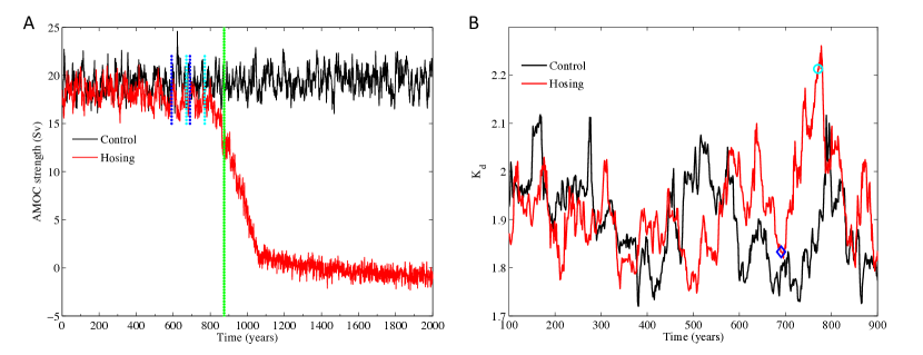
Figure 9: (A) Time series of the annual mean MOC (in Sv, 1 Sv = 10⁶ m³s^-1) at 26^∘N and 1000m depth in the Atlantic for the control simulation (black curve) and the hosing simulation (red curve) of the FAMOUS model. The green line indicates the collapse time $\tau_{c}=874$ years. (B) The kurtosis indicator $K_{d}$ gives an early warning signal of the collapse at 738 years and lasts for 44 years. The blue diamond marker shows the $K_{d}$ value for the window of years 591–690 as indicated by blue dashed lines in panel (A), and the cyan marker shows $K_{d}$ for years 671–770 as indicated by cyan dashed lines in panel (A).

One climate transition of crucial interest is the possible collapse of the Atlantic Meridional Overturning Circulation (MOC) (Mheen et al., 2013; Feng, Viebahn, and Dijkstra, 2014) as is occurring in simulations of the Fast Met Office/UK Universities Simulator (FAMOUS) climate model (Hawkins et al., 2011). Figure 9A shows time series of annual mean Atlantic MOC strength for both the control simulation (black curve) and the hosing simulation (red curve), at the location where the maximum MOC occurs (at latitude 26^∘N and 1000 m depth). The hosing simulation performed using the FAMOUS model is a freshwater-perturbed experiment, in which the freshwater influx over the extratropical North Atlantic is increased linearly from 0.0 Sv to 1.0 Sv (1 Sv = 10⁶ m³s^-1) over 2000 years (Hawkins et al., 2011). One can see that the MOC values of the control simulation are statistically stationary over the 2000-year integration period, while the MOC values for the hosing simulation show a rapid decrease between the years 800 and 1050. Based on a threshold criterium it was found that the MOC collapses at $\tau_{c}=874$ years (Feng, Viebahn, and Dijkstra, 2014), as is shown by the green line in Fig. 9A.

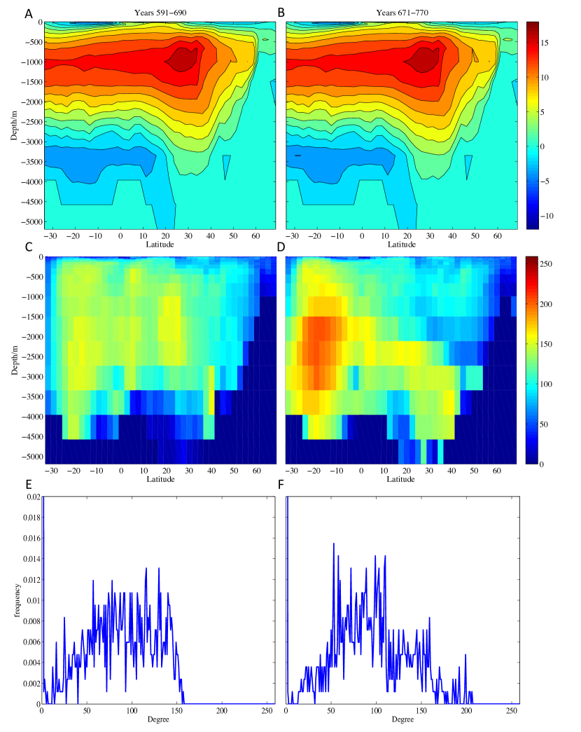
Figure 10: (A,B) Mean MOC stream function pattern over two 100 year windows (years 591–690 and years 671–770). (C,D) Degree field of the Pearson Correlation Climate Network (PCCN) constructed from the MOC data over each window using a threshold value of $\tau=0.5$. (E,F) Degree frequency distribution for both cases.

In Feng, Viebahn, and Dijkstra (2014), PCCNs were reconstructed from the MOC field of the FAMOUS model using a 100-year sliding window (with a time step of one year). It was found that the kurtosis $K_{d}$ of the climate network’s degree distribution (TsonisClimateNetwork.degree_distribution) is a useful early warning indicator for the collapse. The values of $K_{d}$ for the hosing simulation (red curve) and for the control simulation (black curve) are plotted in Fig. 9B. For the hosing simulation, there is indeed a strong increase of $K_{d}$ significantly exceeding the values for the control simulation at 738 years. The classical critical slowdown indicators like variance and lag-1 auto-correlation based on the same MOC data (using the same sliding window) do not show any early warning signal of the MOC transition before the collapse time $\tau_{c}$ (Feng, Viebahn, and Dijkstra, 2014).

To see why the kurtosis $K_{d}$ of the degree distribution of PCCNs is an effective indicator for the Atlantic MOC collapse, we show in Fig. 10 the mean MOC fields (A,B), the degree fields of the PCCNs (C,D) and the degree distribution (E,F) for two 100-year windows (years 591–690 and years 671–770) near the transition. Although the MOC is gradually weakening with the freshwater inflow, the changes in the MOC pattern are relatively minor. However, the changes in the degree field are substantial and when the freshwater inflow is increased, high degrees in the network appear at nodes in the deep ocean (at about 1000 m depth) at mid-latitudes, especially in the South Atlantic. The histograms of the degree fields (the degree distributions) for these windows (Fig. 10E,F) show a tendency towards high degree, which is successfully captured by the kurtosis $K_{d}$.

The collapse of the Atlantic MOC has been identified as one of the important tipping points in the climate system (Lenton et al., 2008), as it will lead to a significantly reduced northward heat transport (Bryan, 1986; Rahmstorf, 2000). With the tools of pyunicorn, we have provided a novel early warning indicator based on climate networks. The particular advantage of such an indicator, in contrast to the indicators based on a single-point time series, is that it reflects spatial correlations. When applied to data from the FAMOUS model, our results show that this kurtosis indicator $K_{d}$ provides a strong early warning signal at least 100 years before the transition.

III.2.2 Use case: seasonal and evolving climate network analysis of monsoon variability

Temporal and spatial variability of climate, and thus climate network structure, are of increasing interest considering ongoing environmental changes. Functional climate networks evolving in time are a promising and useful tool for analyzing spatial and temporal transitions in climate and various other climatic phenomena (Rehfeld et al., 2012; Radebach et al., 2013; Gozolchiani et al., 2008). In particular, evolving climate networks have been used to study seasonal and annual variability of the Indian Monsoon system as one of the major global climatic subsystems affecting life and prosperity of 1/4th of the world’s human population (Malik et al., 2011; Stolbova et al., 2014; Tupikina et al., 2014). On seasonal time scales, it is crucial to identify spatial structures of synchronicity of extreme rainfall events over the Indian monsoon domain, as extreme rainfall events are the main cause of devastating floods on the subcontinent. On annual time scales, variability of the surface air temperature (SAT) field is of great interest, as it influences the total amount of rainfall and its spatial distribution during the monsoon season.

Data and methodology for network construction

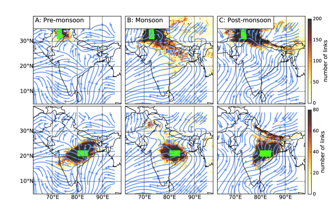
Figure 11: Maps of the number of outgoing undirected links (indicated by color scale) from a set of 153 reference grid points (green rectangles), representing synchronization of extreme rainfall events, and the mean surface wind vector (seasonal, 1998–2012), the latter indicated by blue arrows. The reference regions are: North Pakistan (top panels) and the Eastern Ghats (bottom panels).

In order to study seasonal extreme rainfall variability, we used observational satellite daily rainfall data for the period 1998 – 2012 (TRMM 3B42V7 (Huffman et al., 2007; TRMM, 2012) with a spatial resolution of 0.25^∘ $\sim$ 25 km, extracted for the South Asian region (62.375–97.125^∘ E, 5.125–39.875^∘ N)). First, we defined time series of extreme rainfall events by considering daily precipitation above the 90th-percentile for each rainfall time series as extreme. Then, we constructed seasonal climate networks for three time periods: pre-monsoon (March–May), monsoon (June–September) and post-monsoon seasons (October–December) using event synchronization (Quian Quiroga, Kreuz, and Grassberger, 2002; Boers et al., 2014) – a measure of synchronicity of extreme rainfall events between a pair of geographical locations (climate.EventSynchronizationClimateNetwork class).

For the analysis of annual SAT variability over the Asian monsoon domain we used daily temperature anomaly data (NCEP/NCAR reanalysis (Kistler et al., 2001) for the Asian monsoon region 57.5–122.5^∘ E, 2.5–42.5^∘ N) and construct yearly climate networks for the period 1970–2010 based on Pearson correlation at zero lag using the climate.TsonisClimateNetwork class. We consider a set of 40 static networks obtained from thresholded correlation matrices as one time evolving temporal climate network of the Asian Monsoon domain.

Temporal network measures

For analyzing the annual variability of climate networks of the Asian monsoon domain, we use standard network measures  (Newman, 2003) for quantifying changes in time evolving networks (Holme and Saramäki, 2012), as described in Radebach et al. (2013); Tupikina et al. (2014). Specifically, we calculate average path length $\mathcal{L}$ (TsonisClimateNetwork.average_path_length) and transitivity $\mathcal{T}$ (TsonisClimateNetwork.transitivity) for each time step in the temporal climate network.

Results

Analysis of seasonal networks of extreme rainfall events revealed two key regions, North Pakistan and the Eastern Ghats, which influence the distribution and propagation of extreme rainfall over the Indian subcontinent (Fig. 11). The Eastern Ghats region was previously known by climatologists as an area influencing rainfall over the Indian subcontinent due to its topography, causing orographic rainfall. However, the complex climate network approach allows us to obtain new insights into the climatology of extreme rainfall events and to detect a previously unknown influential region: North Pakistan. This finding pinpoints the strong influence of climatological phenomena such as western disturbances on extreme rainfall events over the Indian subcontinent. It opens new possibilities to account for North Pakistan as a key region for inferring interactions between the Indian Summer Monsoon system and western disturbances, and based on this information, to improve the forecasting of extreme rainfall events over the Indian subcontinent (Stolbova et al., 2014).

Analysis of the annual variability of the evolving Asian monsoon SAT climate network allows us to conclude that a highly non-random, deterministic general structure is present in the network on which the inter-annual variability is imprinted (Radebach et al., 2013; Molkenthin et al., 2014a; Tupikina et al., 2014). The annual climate network variability could be explained by a dominant influence of the topography of the region on the climate network as well as regular monsoon effects, or by dominant climatic events such as El Niño or La Niña (Gozolchiani et al., 2008; Tsonis and Swanson, 2008; Berezin et al., 2012). Observing the changes in temporal climate network properties such as average path length $\mathcal{L}$ and transitivity $\mathcal{T}$ allows to investigate this question further (Fig. 12). Most of the peaks of $\mathcal{L}$ correspond to big El Niño (EN) years, while troughs of $\mathcal{T}$ correspond to La Niña years according to classification of EN in Kug et al. (2009). This coincides well with results concerning the annual variability of global temporal climate networks (Radebach et al., 2013) and indicates the presence of teleconnections between El Niño and Indian Monsoon region.

Figure 12: Evolving average path length $\mathcal{L}$ (A) and transitivity $\mathcal{T}$ (B) network measures calculated for each yearly time step in the temporal climate network constructed for the period (1970–2010). Most of the peaks of $\mathcal{L}$ correspond to big El Niño (EN) years (red vertical bars), troughs of $\mathcal{T}$ correspond to La Niña events (blue vertical bars) where color intensity of the bar corresponds to EN event strength. The data has spatial resolution $2.5^{\circ}\times 2.5^{\circ}$ covering the area between 2.5^∘S to $42.5^{\circ}$N and 57.5^∘E to 122.5^∘, i.e. 468 nodes.

Conclusions

Understanding the variability and evolution of the Indian monsoon and its interactions with ENSO remains one of the most vital questions in climatology. Using the pyunicorn toolbox we were able to analyze these phenomena and their interactions from a climate network perspective. Following this approach revealed the influence of western disturbances and westerlies on the synchronicity, spatial structure and seasonal dynamics of extreme rainfall events over the Indian subcontinent and yielded insights into the annual evolution of temperature climate networks over the Indian monsoon domain, and the influence of ENSO on the Indian monsoon system.

III.3 Coupled climate networks

Coupled climate networks (Donges et al., 2011a; Feng et al., 2012) generalize climate network analysis to the statistical interdependency structures between two or more fields of climatological observables as a network of interacting networks (Fig. 4) and, hence, provide a complementary approach and generalization of classical methods of eigen analysis such as maximum covariance analysis (Donges et al., 2015a). pyunicorn provides the functionality to construct and analyze coupled climate networks via the CoupledClimateNetwork class, which inherits from ClimateNetwork and InteractingNetworks. In accordance with the n.s.i. framework (Sect. II.4), weighted versions of all measures are also available in these classes, e.g. allowing for an area-weighted computation of all interacting network measures (Wiedermann et al., 2013). This is particularly useful when studying coupled climate networks that cover areas close to the poles, as in most cases the density of nodes in these areas varies strongly due to the regular gridding of many climate data sets (e.g. Fig. 6).

We have applied the coupled climate networks framework to study ocean-atmosphere interactions in the Northern hemisphere based on the monthly HAD1SST sea-surface temperature (SST) (Rayner et al., 2003) and the 500 mbar geopotential height (HGT) fields from the ERA40 reanalysis project (Uppala et al., 2005) for all nodes northward of $30^{\circ}$N latitude and using the linear Pearson correlation coefficient at zero lag (Wiedermann et al., 2015b).

Local interacting network measures allow for the detection of regions in one field that couple with the other field and additionally provide a notion of the resulting coupling strength and structure (Fig. 13). The n.s.i.  cross-degree density

$$\kappa_{v}^{ij\ast} =\frac{1}{W_{j}}\sum_{q\in V_{j}}w_{q}A_{vq}^{+}$$ (17)

$$=\frac{1}{W_{j}}k_{v}^{ij\ast}$$ (18)

measures the weighted share of nodes in another subnetwork $V_{j}$ that each node $v\in V_{i}$ is connected with. It is obtained by normalizing the n.s.i.  cross-degree $k_{v}^{ij\ast}$ (InteractingNetworks.nsi_cross_degree) by the sum over all node weights in the opposite subnetwork $W_{j}=\sum_{q\in V_{j}}w_{q}$ such that its values range between 0 and 1. Thus, high values indicate a strong localized coupling between the fields or climate subnetworks. Figure 13A shows the n.s.i. cross-degree density $\kappa_{v}^{si\ast}\equiv\kappa_{v}^{i\ast}$ for nodes in the SST field (subnetwork index $s$). We find several localized areas in the Atlantic as well as the Pacific that show strong coupling with the HGT field (subnetwork index $i$). In contrast, the n.s.i cross-degree density $\kappa_{v}^{is\ast}\equiv\kappa_{v}^{s\ast}$ for nodes in the HGT field shows large areas of pronounced coupling with the SST field (Fig. 13B). It should be noted, however, that this measure by definition does not contain any information on the interactions within each of the fields.

Additionally, the n.s.i. local cross-clustering coefficient

$$\mathcal{C}_{v}^{ij\ast} =\frac{\sum_{p,q\in V_{j}}A^{+}_{vp}w_{p}A^{+}_{pq}w_{q}A^{+}_{qv}}{(k_{v}^{ij\ast})^{2}}$$ (19)

indicates whether two neighbors in subnetwork $V_{j}$ of a considered node $v\in V_{i}$ are also mutually connected and, hence, measures the weighted share of triangular structures between both subnetworks. It is computed using the method InteractingNetworks.nsi_cross_local_clustering. We note that generally the n.s.i. cross-local clustering coefficient takes lower values for nodes in the SST field ($\mathcal{C}_{v}^{si\ast}\equiv\mathcal{C}_{v}^{i\ast}$, Fig. 13C) then for nodes in the HGT field ($\mathcal{C}_{v}^{is\ast}\equiv\mathcal{C}_{v}^{s\ast}$, Fig. 13D) implying that nodes in the SST field couple preferably with nodes in the HGT field, which are themselves dynamically dissimilar and, hence, disconnected.

In fact, we find that the ocean-to-atmosphere interaction in the Northern hemisphere follows a hierarchical structure (Ravasz and Barabási, 2003), meaning that larger areas of dynamically similar nodes in the SST field couple with several dynamically dissimilar areas in the HGT field (Wiedermann et al., 2015b). This feature may be attributed to large-scale ocean currents interacting with different parts of the atmosphere along their respective directions of flow.

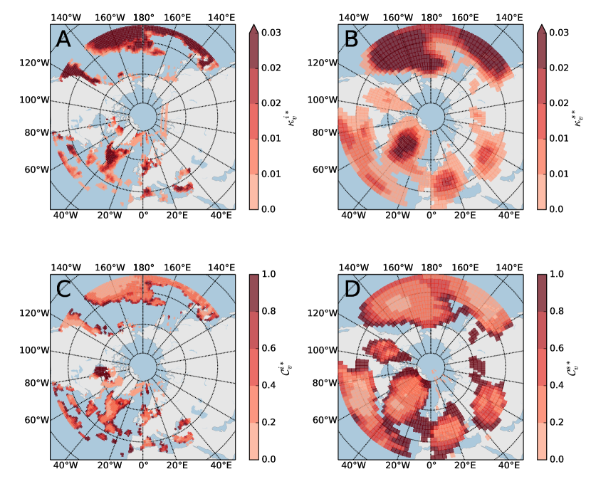
Figure 13: Coupled climate network analysis of ocean-atmosphere interactions northward of 30^∘ N: N.s.i. cross-density (A) for nodes in the sea surface temperature field and (B) for nodes in the geopotential height field at 500 mbar. (C, D) The same for the n.s.i. local cross-clustering coefficient.

IV Network-based time series analysis

Network-based methodologies provide valuable novel approaches to nonlinear time series analysis that have manifold applications ranging from studying the detailed geometrical structure of a dynamical system in phase space to detecting critical transitions or tipping points in observational time series (Xu, Zhang, and Small, 2008; Donner et al., 2011a). While time series networks can reflect the dynamical properties of time series obtained from a complex system in a smorgasbord of different ways, pyunicorn focusses on two complementary approaches: (i) Recurrence networks (Marwan et al., 2009; Donner et al., 2010), an approach closely related to recurrence quantification analysis of recurrence plots, are random geometric graphs (Dall and Christensen, 2002; Donges et al., 2012) representing proximity relationships (links) of state vectors (nodes) in phase space (Sect. IV.1). (ii) Visibility graphs encode visibility relations between data points in the one-dimensional time domain (Sect. IV.2; Lacasa et al. (2008); Donner and Donges (2012)). Hence, while recurrence networks allow to investigate geometric properties of the system such as the transitivity dimension (Donner et al., 2011b), visibility graphs can be applied to investigate purely temporal features such as long-range correlations (Lacasa et al., 2009) or time-reversal asymmetry (Donges, Donner, and Kurths, 2013). Network-based time series analysis is demonstrated by discussing two use cases from paleoclimatology that aim at detecting regime shifts or tipping points in climate dynamics on longer time-scales.

IV.1 Recurrence analysis

Recurrence is a fundamental property of many dynamical systems and is used by several approaches in order to investigate a system’s dynamics. A basic tool of nonlinear time series analysis is the binary recurrence matrix (Marwan et al., 2007)

$$R_{pq}(\varepsilon)=\Theta(\varepsilon-||\mathbf{x}(p)-\mathbf{x}(q)||),$$ (20)

where $\mathbf{x}(p)$ is a state vector at time $p=1,\ldots,N$, $N$ the number of states, $\Theta(\cdot)$ again the Heaviside function, and $\varepsilon$ the recurrence threshold. A graphical representation, the recurrence plot, provides visual, qualitative impressions about the dynamics of even high-dimensional systems. Quantitative approaches based on this matrix have been developed for studying different aspects of complex systems, particularly based on univariate and multivariate time series data (Marwan et al., 2007). Recurrence quantification analysis (RQA) and recurrence network analysis (RNA) allow to classify different dynamical regimes in time series and to detect regime shifts, dynamical transitions or tipping points, among many other applications (Marwan and Kurths, 2015). Bivariate methods such as joint recurrence plots/networks, cross-recurrence plots or inter-system recurrence networks can be used to investigate the coupling structure between two dynamical systems based on their time series, including methods to detect the directionality of coupling (Romano et al., 2007; Zou et al., 2011; Feldhoff et al., 2012). Recurrence analysis is applicable to general time series data from many fields such as climatology, medicine, neuroscience or economics (Marwan, 2008). These applications range from using recurrence analysis as a classifier for monitoring health states in medicine and engineering (Ramírez Ávila et al., 2013) to detecting continental-scale nonlinear regime shifts in the Asian monsoon system during the Holocene (Donges et al., 2015b).

IV.1.1 Recurrence quantification analysis

Recurrence of a dynamical system is usually studied in phase space. A standard approach is to use time-delay embedding for reconstructing the appropriate phase space representation from a measured time series (Packard et al., 1980).

The class timeseries.RecurrencePlot can be used to generate recurrence plots and perform recurrence quantification analysis. The parameters dim and tau can be used to set the parameters of the time-delay embedding, whereas threshold or recurrence_rate as well as metric configure the recurrence criteria (i.e. used recurrence norm and threshold $\varepsilon$). The method RecurrencePlot.embedding can be used to get the reconstructed phase space vectors resulting from the specified embedding parameters. For example, a recurrence plot can be computed from a given scalar time series $x(t)$ using the following code:

rp = RecurrencePlot(x, recurrence_rate=0.05,
dim=3, tau=30)

The recurrence matrix $\mathbf{R}$ (Eq. 20) can be extracted as the property RecurrencePlot.R and can be plotted (Fig. 14), e.g. using matplotlib, or used for subsequent analysis.

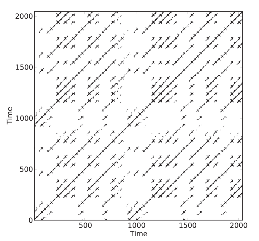
Figure 14: Recurrence plot of a time series generated by the Lorenz ’63 system in a chaotic regime (Lorenz, 1963).

The simplest quantifier in recurrence analysis is the probability that any recurrence will occur, i.e. the fraction positive entries in $\mathbf{R}$, called recurrence rate (RecurrencePlot.recurrence_rate). However, information about dynamical properties of the system is represented by the diagonal and vertical lines apparent in the recurrence plot. The line length distributions are, thus, the foundation for statistical, quantitative analysis of the recurrence matrix $\mathbf{R}$ (Eq. (20)), called recurrence quantification analysis (Marwan et al., 2007). Moreover, the empty vertical spaces in $\mathbf{R}$, apparent as white vertical lines in the recurrence plot, correspond to recurrence times. Several measures of complexity using these line distributions (diagonal, vertical, and white lines) are available as methods in the RecurrencePlot class, e.g. maximal diagonal line length (max_diaglength), determinism (determinism), laminarity (laminarity), diagonal line entropy (diag_entropy) or mean recurrence time (mean_recurrence_time). The distributions of diagonal and vertical lines (diagline_dist and vertline_dist) can be useful for further quantifications, e.g. by looking at the scaling behavior, which is related to the $K_{2}$ entropy (Marwan et al., 2007). Resampled instances of both types of line distributions can be generated using the methods resample_diagline_dist and resample_vertline_dist for estimating confidence bounds for RQA measures following the permutation-based method proposed by (Schinkel et al., 2009).

pyunicorn furthermore supports multivariate extensions of RQA such as joint (timeseries.JointRecurrencePlot) and cross recurrence plots (timeseries.CrossRecurrencePlot) that both inherit from the RecurrencePlot class.

IV.1.2 Recurrence network analysis

The striking similarity of the binary square recurrence matrix (Eq. 20) with the adjacency matrix (Eq. 1) of an unweighted and undirected network has lead to a complementary kind of recurrence analysis by measures from complex network studies (Marwan et al., 2009; Donner et al., 2010). More formally, the recurrence networks (Fig. 15) defined in this way by their adjacency matrix

$$A_{pq}(\varepsilon)=R_{pq}(\varepsilon)-\delta_{pq},$$ (21)

where $\delta_{pq}$ is Kronecker’s delta introduced to avoid self-loops in the networks, can be understood as random geometric graphs (Fig. 15) that capture rich information on the geometrical structure of a dynamical system’s invariant density in phase space (Dall and Christensen, 2002; Donges et al., 2012). The nodes in a recurrence network represent state vectors and the links indicate proximity relationships between them. Recurrence networks are represented by the timeseries.RecurrenceNetwork class inheriting from Network and RecurrencePlot (Fig. 1A).

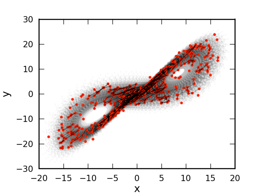
Figure 15: Recurrence network as a random geometric graph generated from $N=750$ state vectors (red filled circles) drawn from the invariant density of the Lorenz ’63 system in a chaotic regime (Lorenz, 1963). In this example, state vectors (nodes) with a distance smaller than $\varepsilon=2$ according to the supremum norm are connected by a link.

This approach opens up the wealth of measures, models and algorithms from complex network theory for time series analysis. Network measures such as average path length (Network.average_path_length), global clustering coefficient (Network.global_clustering), transitivity (Network.transitivity) or assortativity (Network.assortativity) characterize the geometrical properties of the dynamical system trajectories in phase space and can be used to differentiate between dynamical regimes,e.g. periodic and chaotic (Marwan et al., 2009; Donner et al., 2010; Zou et al., 2010). In particular, the transitivity

$$\mathcal{T}(\varepsilon)=\frac{\sum_{v,p,q\in V}A_{vp}(\varepsilon)A_{pq}(\varepsilon)A_{vq}(\varepsilon)}{\sum_{v,p,q\in V}A_{vp}(\varepsilon)A_{vq}(\varepsilon)}$$ (22)

is appropriate because it can be linked to the geometry of the phase space trajectory (Donner et al., 2011b; Donges, 2012). Specifically, it can be logarithmically transformed to yield the single-scale transitivity dimension

$$D_{\mathcal{T}}(\varepsilon)=\frac{\log\mathcal{T}(\varepsilon)}{\log(3/4)},$$ (23)

a global dimension-like measure of the geometric organization of the available set of state vectors in phase space (RecurrenceNetwork.transitivity_dim_single_scale). Analogously, a transformed local clustering coefficient yields a local dimension-like measure that is defined on every node or state vector (RecurrenceNetwork.local_clustering_dim_single_ scale).

Analogously to multivariate RQA (Sect. IV.1.1), multivariate extensions of recurrence network analysis have been applied to investigate directions of coupling between dynamical systems (Feldhoff et al., 2012) and complex synchronization scenarios including generalized synchronization (Feldhoff et al., 2013). The corresponding methodologies are represented by the classes timeseries.InterSystemRecurrenceNetwork and timeseries.JointRecurrenceNetwork, respectively.

IV.1.3 Use case: identification of transitions in paleoclimate variability

A relevant application of recurrence analysis is the detection of dynamical transitions in complex systems captured by model or observational time series (Marwan et al., 2009; Donges et al., 2011b). Detecting such dynamical transitions, regime shifts or tipping points (Lenton et al., 2008; Rockström et al., 2009) is of great interest in studying past climate variability to gain a deeper understanding of the Earth’s climate system also on geological time scales (Donges et al., 2011c, 2015b). In the following we discuss a typical example from paleoclimate research following Marwan and Kurths (2015) that focusses on investigating interactions between sea-surface temperature (SST) and the dynamics of specific climate subsystems, such as the Asian monsoon system or the Atlantic thermohaline circulation, as well as regime shifts therein.

Diverse types of geological archives are used in paleoclimatology to reconstruct and study climate conditions of the past, such as lake (Marwan et al., 2003) and marine sediments (Herbert et al., 2010; Donges et al., 2011b, c) or speleothems (Kennett et al., 2012; Donges et al., 2015b). Alkenone remnants in the organic fraction of marine sediments, produced by phytoplankton, can be used to reconstruct SSTs of the past (alkenone paleothermometry), which allows to investigate past oceanic temperature variability (Herbert, 2001; Li et al., 2011). In this use case, we analyze an SST reconstruction for the South China Sea covering the past 3 Ma that is derived from alkenone paleothermometry of the Ocean Drilling Programme (ODP) site 1143 drill core (Li et al., 2011) (Fig. 16A). The South China Sea is strongly connected to the East Asian Monsoon (EAM) system encompassing a winter monsoon season with strong winds and a summer monsoon season with particularly high precipitation.

We generate RecurrenceNetwork objects and compute the measures determinism DET (RecurrenceNetwork.determinism) and transitivity $\mathcal{T}$ (RecurrenceNetwork.transitivity) for sliding windows of length 410 ka (containing a varying number of data points due to the time series’ irregular sampling) and a step size of 20 ka (Fig. 16B). For reconstructing the phase space by time-delay embedding (Packard et al., 1980), we select an embedding dimension of $6$ (as suggested by the false nearest neighbors criterion (Kennel, Brown, and Abarbanel, 1992)). The selection of the time-delay parameter is guided by the auto-correlation function. As a result, it is approximated as 20 ka for all time windows based on the median sampling time within each window. The recurrence threshold is chosen to preserve a prescribed recurrence rate of 7.5% (Marwan et al., 2007; Donges et al., 2011c).

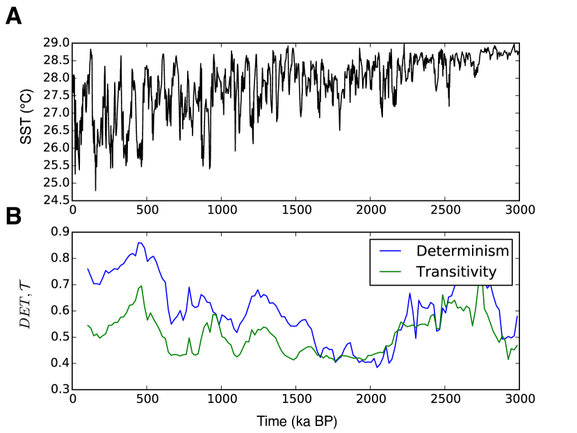
Figure 16: Studying dynamical transitions in paleoclimate data using recurrence analysis: (A) Alkenone paleothermometry based SST estimates for the South China Sea and (B) corresponding determinism DET and transitivity $\mathcal{T}$.

During the past 3 Ma, several major and many smaller climate changes occurred on regional, but also global scales. Particularly pronounced climate shifts have been related to Milankovich cycles (Haug and Tiedemann, 1998; Medina-Elizalde and Lea, 2005; An et al., 2014) and major changes in ocean circulation patterns (Karas et al., 2009). Following a transition towards obliquity-driven climate variability with a 41 ka period around 3.0 Ma BP (before present), a long period of globally warm climate ended and Northern hemisphere glaciations started after 2.8–2.7 Ma BP (Haug and Tiedemann, 1998; Herbert et al., 2010; An et al., 2014). This transition is revealed by a significant increase of DET and $\mathcal{T}$ between 2.8 and 2.2 Ma signifying an increased regularity of SST dynamics during this period. From detailed studies of loess sediments it is known that around 1.25 Ma BP, the intensity of the EAM winter monsoon season started to be strongly coupled to global ice-volume change (An et al., 2014). Around this time also marking the beginning of a transition phase towards glacial-interglacial cycles of 100 ka period (eccentricity-dominated period of the Milankovich cycles), DET and $\mathcal{T}$ increase markedly again. Dominance of the 100 ka period was well established after 0.6 Ma and is clearly indicated by increased DET and $\mathcal{T}$ values between 0.6 and 0.2 Ma BP (Sun et al., 2010). It is also known from loess sediments that the EAM summer monsoon weakened between 2.0 and 1.5 Ma BP and around 0.7 Ma BP. During these periods, DET and $\mathcal{T}$ assume lower values and, hence, more irregular SST variability, than during the previously discussed epochs.

In this way, recurrence analysis by means of the measures DET and $\mathcal{T}$ confirms earlier findings of strong links between the EAM and Milankovich cycles. Furthermore, the analysis of recurrence properties allows for deeper insights, such as that dominant Milankovich cycles and periods of major climate transitions from one to another regime go along with increased and reduced regularity in the (regional) climate dynamics in the East Asian Monsoon system (as reflected by the South China Sea SST and for the considered time scales).

IV.2 Visibility graphs

Visibility graph (VG) methods represent an alternative approach for transforming time series into complex networks (Lacasa et al., 2008), which draws upon analogies between height profiles in physical space and the profile of a time series graph. Originally utilized in fields like architecture and robot motion planning, VGs are based on the existence or non-existence of lines of sight between well-defined objects.

IV.2.1 Theory of time series visibility graphs

In a time series context, these objects are the sampling points of a (univariate) time series graph, which are uniquely characterized by pairs $(t_{v},x_{v})$ with $x_{v}=x(t_{v})$. From a practical perspective, we can identify each node $v$ of a standard visibility graph with a given time point $t_{v}$. For $t_{v}<t_{p}$ (and, hence, $v<p$) a link between the nodes $v$ and $p$ exists iff

$$x_{q}<x_{v}+\frac{x_{p}-x_{v}}{t_{p}-t_{v}}(t_{q}-t_{v})\ \forall\ v<q<p.$$ (24)

Put differently, the topological properties of VGs are closely related to the roughness of the underlying time series profile.

As a notable algorithmic variant, horizontal visibility graphs (HVGs) facilitate analytical investigations of the graph profile (Luque et al., 2009). In this case, Eq. (24) is replaced by the simpler condition

$$x_{q}<\min\{x_{v},x_{p}\}\ \forall\ v<q<p.$$ (25)

One easily convinces oneself that the latter condition is more restrictive, and that the link set of a HVG is a subset of that of the standard VG. In turn, the classical VG is invariant under arbitrary affine transformations of a time series, whereas the HVG retains this invariance only for uniform translations and rescaling of the original data.

In pyunicorn, VG and HVG can be generated from any time series object via the timeseries.VisibilityGraph class. The decision on which of the two variants is used is mediated via the Boolean parameter horizontal, which can be set to False (standard VG, default value) or True (HVG). Additional information on the timings of individual observations as well as missing values can be provided via supplementary optional parameters.

The distinctively different construction mechanism of (H)VGs in comparison to recurrence networks (Sect. IV.1.2) implies a completely different interpretation of the resulting networks. First, recurrence networks are equally applicable to uni- and multivariate time series, whereas VGs are tailored for applications to univariate records. So far, there is no way to unambiguously generalize the VG concept to bi- or multivariate time series.

Second, both types of time series networks are spatial networks (Sect. II.2) in an abstract sense - recurrence networks’ nodes being characterized by the positions of the associated state vectors in the dynamical system’s phase space, and those of VGs being fixed along the time axis representing some abstract one-dimensional space. This fact implies strong restrictions to the resulting graph properties (Donner and Donges, 2012), including potentially severe biases of (especially path-based) network properties due to the absence of information prior to the first, as well as after the last sampling point of the time series. To this end, simplified functionalities correcting for such effects have been implemented for the case of degree and closeness centrality measures (boundary_corrected_degree and boundary_corrected_closeness, respectively). An improved treatment is planned for future releases of pyunicorn, but still requires further analytical understanding of the VG properties.

Third, while power-law degree distributions of recurrence networks are related with specific singularities of the probability density of states (Zou et al., 2012), they are a widely observable feature of VGs that arises from the presence of long-range correlations (Lacasa et al., 2009; Ni, Jiang, and Zhou, 2009). Specifically, under the assumption of a fractional Brownian motion or related stochastic process, the characteristic scaling exponent of the degree distribution of a VG can be directly related with the Hurst exponent of the series, whereas there are no similar unique relationships for recurrence networks (Zou et al., 2012). However, given the multiplicity of existing estimators of the latter quantity, the practical advantage of using VGs and HVGs for this purpose has not yet been convincingly demonstrated.

Finally, given the direct association between nodes and time points, VGs and HVGs provide a means to discriminate the statistical properties of a graph when looking forward and backward in time, respectively, from a given observation point. This gives birth to a new class of time series irreversibility tests (Lacasa et al., 2012; Donges, Donner, and Kurths, 2013), which allow to evaluate the null hypothesis of linearity since irreversibility is a common hallmark of nonlinear dynamics (Theiler et al., 1992). Specifically, local (node-wise) graph properties can be decomposed into contributions from either past or future observations (retarded (backward) vs. advanced (forward)), as well as such combining information from past and future (trans). Corresponding features are implemented in pyunicorn for a variety of network properties, including degree (retarded_degree vs. advanced_degree), local clustering coefficient (retarded/advanced_local_clustering), closeness (retarded/advanced_closeness) and betweenness (retarded/advanced/trans_betweenness).

IV.2.2 Use case: time irreversibility in glacial-deglacial dynamics

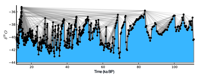
Figure 17: Visibility graph of the GISP2 ice core $\delta^{18}O$ record (2m resolution) from Greenland during the last glacial (Grootes and Stuiver, 1997). Black dots indicate observations (nodes). Links are added between mutually visible observations (gray lines).

VG-based tests for time series irreversibility have been successfully applied to discriminate between different dynamical regimes in EEG recordings from healthy and epileptic patients (Donges, Donner, and Kurths, 2013). It is instructive to also apply this methodology to study regime shifts in paleoclimate dynamics (Schleussner et al., 2015), particularly for investigating in depth the important differences between interglacial and glacial climate variability and the nature of the transitions between those regimes (Donges, 2012). As an example, we study the 2 m resolution $\delta^{18}O$ isotope record from the GISP2 ice core from Greenland (Grootes and Stuiver, 1997) convering both the Holocene and the last glacial period (Fig. 17). The boundary between the last glacial and the Holocene is defined by the Younger Dryas-Preboreal transition at about 11,650 years BP (Grootes and Stuiver, 1997).

We apply the test for time irreversibility proposed in Donges, Donner, and Kurths (2013), which is based on comparing the distributions of time-directed degree (VisibilityGraph.retarded/advanced_degree)

$$k_{v}^{r} =\sum_{p\in V:p<v}A_{vp},$$ (26)

$$k_{v}^{a} =\sum_{p\in V:p>v}A_{vp}$$ (27)

and time-directed local clustering coefficient (VisibilityGraph. retarded/advanced_local_clustering)

$$\mathcal{C}_{v}^{r} ={k_{v}^{r}\choose 2}^{-1}\sum_{p,q\in V:p,q<v}A_{vp}A_{pq}A_{qv},$$ (28)

$$\mathcal{C}_{v}^{a} ={k_{v}^{a}\choose 2}^{-1}\sum_{p,q\in V:p,q>v}A_{vp}A_{pq}A_{qv}.$$ (29)

using the Kolmogorov-Smirnov test. To ensure the robustness of the results, a $k$-leave-out cross-validation is conducted by generating ensembles of $100$ realizations for each record by bootstrapping 80% of the data points without changing their time ordering and, subsequently, performing the test to each ensemble member. Following this protocol for the Holocene and the last glacial period time series segments separately, we find that the null hypothesis of reversibility can be quite safely rejected for the last glacial, whereas this is not the case for the Holocene (Tab. 2). Since the conditions for the deposition of ice and snow at the drilling site are argued to have remained more or less constant throughout the entire time span covered by the record, these results point at a strong signature of nonlinear climate dynamics during the last glacial, which is not detected for the Holocene, consistently with results for Holocene speleothem records (Donges, 2012). One visually directly accessible piece of evidence for the indicated irreversible dynamics during the last glacial period are the frequently occurring Dansgaard-Oeschger events that are characterized by rapid warming (change towards more positive $\delta^{18}O$ values) and subsequent slower cooling (change towards more negative $\delta^{18}O$ values) of Greenland climate (Fig. 17). Note that the sampling times increase with age for the GISP2 as for all ice core proxy records (in GISP2, the average sampling time is $14.2\pm 6.3$ a for the Holocene, while it is $175.8\pm 119.6$ a during the last glacial period), because the ice column is compressed by ice and snow deposited on top of it over the years. It remains to be tested in future research whether this nonstationarity has a strong impact on the results of the VG test for time irreversibility.

Table 2: Results of the visibility graph-based tests for time irreversibility of the GISP2 ice core $\delta^{18}O$ record from Greenland (Grootes and Stuiver, 1997). The number of data points in each time series segment is denoted by $M$, while $q_{k}$ and $q_{\mathcal{C}}$ give the rate of rejection for the null hypothesis of time reversibility (at a 95% significance level) during a $k$-leave-out cross-validation for degree and clustering-based tests, respectively.

Period	Time span (ka BP)	M	$q_{k}$	$q_{\mathcal{C}}$
Last glacial	110.98 – 11.65	$566$	$0.93$	$0.82$
Holocene	11.65 – today	$824$	$0.00$	$0.00$

V Surrogate time series

As mentioned in several contexts above and analogously to random network models (see, e.g. Sect. II.2 on random surrogate models for spatial networks and Sect. II.3 on surrogate models for networks of networks), surrogate time series are a useful methodology for testing the statistical significance of observed time series properties such as those derived from functional networks or network-based time series analysis based on various null hypotheses (Schreiber and Schmitz, 2000). The idea behind this approach is to generate surrogate time series that conserve certain properties of observed time series such as the amplitude distribution or auto-correlation function, but are random otherwise. pyunicorn can be used to generate several commonly used types of time series surrogates (timeseries.Surrogates class): white noise surrogates, Fourier surrogates, amplitude adjusted Fourier transform surrogates (Schreiber and Schmitz, 2000) or twin surrogates (Thiel et al., 2006). White noise surrogates correspond to randomly shuffled copies of a time series $x(t)$ and, hence, retain only the amplitude distribution of the original data (Surrogates.white_noise_surrogates). In contrast, Fourier surrogates are generated by randomizing the phase components of $x(t)$ in Fourier space and conserve the time series’ power spectrum (and thus also its linear auto-correlation function via the Wiener-Chintschin theorem), but not the amplitude distribution (Surrogates.correlated_noise_surrogates). This potential drawback is addressed by amplitude adjusted Fourier transform (AAFT) surrogates that only approximate the power spectrum but conserve the amplitude distribution (Surrogates.AAFT_surrogates). An even closer match is provided by iteratively refined AAFT surrogates (Surrogates.refined_AAFT_surrogates). Finally, twin surrogates approximate the recurrence structure of the original time series and, hence, have the potential to additionally conserve certain nonlinear properties of $x(t)$ such as the auto-mutual information function (Surrogates.twin_surrogates). Note that the surrogate types supported by pyunicorn only conserve certain properties of single time series, whereas multivariate surrogate methods (Schreiber and Schmitz, 2000) conserving properties of pairs of time series such as the linear cross-correlation function are currently not implemented.

When computing functional networks, surrogate time series can be used to include links in the network based on a fixed significance level instead of a fixed threshold or link density in terms of the considered similarity measure from coupling analysis (see, e.g. Paluš et al. (2011)). In network-based time series analysis, surrogate time series provide a means to test the statistical significance of results obtained for the data at hand based on a hierarchy of null hypotheses, for example, when searching for dynamical transitions and regime shifts (Donges et al., 2011b, c) or when studying the directionality of coupling or synchronization between time series (Feldhoff et al., 2012, 2013).

VI Conclusions and perspectives

In this article, we have described the pyunicorn software package, which facilitates the study of various types of complex networks as well as a detailed investigation of time series data using modern methods of functional network and network-based nonlinear time series analysis. pyunicorn is written in the programming language Python and, hence, is conveniently applicable to research domains in science and society as different as neuroscience, infrastructure and climatology. Most computationally demanding algorithms are implemented in fast compiled languages on sparse data structures, allowing the performant analysis of large networks and time series data sets. The software’s modular and object-oriented architecture enables the flexible and parsimonious combination of data structures, methods and algorithms from different fields. For example, combining complex network theory (core.Network class) and recurrence plots (timeseries.RecurrencePlot class) yields recurrence network analysis (timeseries.RecurrenceNetwork class), a versatile framework that opens new perspectives for nonlinear time series analysis and the study of complex dynamical systems in phase space. Another example are climate networks (climate.ClimateNetwork class), an approach bringing together ideas and concepts from complex network theory and classical eigen analysis of climatological data (e.g. empirical orthogonal function analysis) (Donges et al., 2015a).

Along these lines, pyunicorn has the potential to facilitate future methodological developments in the fields of network theory, time series analysis and complex systems science by synthesizing existing elements and by adding new methods and classes that interact with or build upon preexisting ones. Nonetheless, we urge users of the software to ensure that such developments are theoretically well-founded and explicable as well as motivated by well-posed and relevant research questions to produce high-quality research.