A Simple Model of Dynamical Supersymmetry Breaking with the Generation of Soft Mass(es)

Abstract

We introduce a simple model of dynamical supersymmetry breaking. It is like a supersymmetric version of a Nambu–Jona-Lasinio model with a spin one composite. The simplest version of the model as presented here has a single chiral superfield (multiplet) with a four-superfield interaction. The latter has the structure of the square of the superfield magnitude square. A vacuum condensate of the latter is illustrated to develop giving rise to supersymmetry breaking with a soft mass term for the superfield. We report also the effective theory picture with a real superfield composite, illustrating the matching effective potential analysis and the vacuum solution conditions for the components. The nature of its fermionic part as the Goldstone mode is presented. Phenomenological application to the supersymmetric standard model is plausible.

I Introduction

Our group has recently re-visited supersymmetric versions of the classic model of dynamical symmetry breaking — the Nambu–Jona-Lasinio (NJL) model NJL . We have formulated an approach to derive the gap equation(s) for the supersymmetric mass parameter(s) including supersymmetry breaking parts 042 . Applying it with a supergraph calculation, we have succeeded in obtaining the model gap equations for both the old supersymmetric Nambu–Jona-Lasinio (SNJL) model BL ; BE and the new holomorphic version (dubbed HSNJL model) we proposed as the alternative supersymmetrization 034 . Along the line of the NJL model idea, the supersymmetric models have dimension five or six four-superfield interactions which in the regime of large enough coupling induce the formation of two-superfield condensates that break some part of the model symmetry and generate masses. In all such cases soft supersymmetry breaking masses are needed. Exact supersymmetry would otherwise protect the model against any dynamical symmetry breaking.

Here in this letter, we report on an even more interesting possibility for the physics of the kind of four-superfield interactions — dynamical breaking of supersymmetry itself with the generation of soft supersymmetry breaking mass(es).

Interesting simple models of spontaneously breaking of supersymmetry are difficult to find rev . A simple model that has the supersymmetry broken dynamically is even more valuable. Apart from of theoretical interest, model of soft supersymmetry breaking could be relevant for TeV scale phenomenology as a background model behind a softly broken supersymmetric standard model (SSM) soft . We have shown that a HSNJL model is a phenomenological viable version of the SSM with the Higgs superfields as dynamical composites of quark superfields 034 . It will be more interesting if the required soft supersymmetry breaking (squark) masses themselves could be the result of the kind of dynamical supersymmetry breaking. A model incorporating such a mechanism may be possible with or even without a single extra superfield beyond that of the (minimal) SSM. In contrast, models in the literature usually require the construction of elaborated supersymmetry breaking and mediating sectors to accomplish the generation of the soft supersymmetry breaking terms soft . The new model mechanism reported here hence provides an interesting alternative with plausible implications for searches at the LHC.

In this letter, we focus on the first step, presenting a prototype model of such a dynamical supersymmetry breaking with a SNJL type four-superfield interaction. We skip most of the details of the calculations here to focus on the key formulational aspects and the main results. For the skipped details and more general analysis, please see our companion long paper 063 . A brief discussion on its possible phenomenological applications will be given at the end.

II The model and the soft mass gap equation

The SNJL model has the four-superfield interaction BL ; BE ; 042

$$g^{2}\int\!\!d^{4}\theta\,\Phi_{+a}^{\dagger}\Phi_{-}^{a\dagger}\Phi_{+}^{b}\Phi_{-b}\,(1-\tilde{m}_{\!\scriptscriptstyle C}^{2}\theta^{2}{\bar{\theta}}^{2})\;,$$ (1)

in which $a$ and $b$ represent the color indices explicitly shown here. As the two-superfield condensate $\left\langle\left.\Phi_{+a}^{\dagger}\Phi_{-}^{a\dagger}\right|_{F}\right\rangle$ develops, Dirac mass for $\Phi_{+}^{b}\Phi_{-b}$ is resulted. Now consider a similar but supersymmetric interaction with an alternative color index contraction as given by

$$g^{2}\int\!\!d^{4}\theta\,\Phi_{+a}^{\dagger}\Phi_{-}^{b\dagger}\Phi_{+}^{a}\Phi_{-b}\;.$$ (2)

One can easily see that if the two-superfield condensate $\left\langle\left.\Phi_{+a}^{\dagger}\Phi_{+}^{a}\right|_{D}\right\rangle$ develops, we will obtain a soft supersymmetry breaking mass for $\Phi_{-}^{b\dagger}\Phi_{-b}$ ( $|_{D}$ denote the component $D$-term, i.e. the $\theta^{2}{\bar{\theta}}^{2}$ part, as commonly used in supersymmetric theories). We analyze here the scenario in the simplest case with only one chiral superfield multiplet, in relation to the question of dynamical supersymmetry breaking. The very naive looking model actually gives a highly nontrivial and not very conventional model Lagrangian in terms of component fields.

Suppressing the color index, the simple model is given with kinetic term, mass term, and the dimension six interaction, i.e. as

$${\cal{L}}=\int d^{4}\theta\,\left[\Phi^{\dagger}\Phi\,+\frac{m}{2}\Phi\Phi\delta^{2}(\bar{\theta})+\frac{m^{*}}{2}\Phi^{\dagger}\Phi^{\dagger}\delta^{2}(\theta)-\frac{g^{2}}{2}\left(\Phi^{\dagger}\Phi\right)^{2}\right]\;.$$ (3)

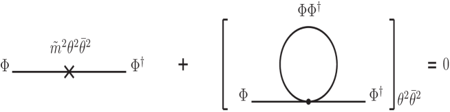
Figure 1: The soft mass gap equation. Only the $\theta^{2}\bar{\theta}^{2}$ component of the superfield amplitude for the second part is to be taken. The other way, to look at it is to see the first part as a $\tilde{m}^{2}$ insertion for $AA^{*}$ and the second part as the $\Phi$-loop amplitude for $AA^{*}$.

 

It is supersymmetric. Note that the four-superfield interaction is written with a sign opposite to that of the old SNJL model, the reason behind which will surface below. Otherwise, one may also look at much of the analysis without restricting to a positive $g^{2}$. The first step of the self-consistent Hartree approximation is to add the interested soft mass term $-\int d^{4}\theta\Phi^{\dagger}\Phi\tilde{m}^{2}\theta^{2}\bar{\theta}^{2}$ to the free field part and re-subtract it as a mass-insertion type interaction. The formal gap equation can be illustrated diagrammatically as in Fig.1, with the analytical expression given by

$$\tilde{m}^{2}=\left.\Sigma_{\tilde{m}}^{\tiny(loop)}(p)\right|_{\mbox{\tiny on-shell}}\equiv-\left.\Sigma^{({\mbox{\tiny}loop})}_{\Phi\Phi^{\dagger}}(p;\theta^{2},\bar{\theta}^{2})\right|_{\theta^{2}\bar{\theta}^{2},\mbox{\tiny on-shell}}\;.$$ (4)

where we have, in accordance with the formulation discussed in Ref.042 , introduced the superfield two-point proper vertex $\Sigma_{\Phi\Phi^{\dagger}}(p;\theta^{2},\bar{\theta}^{2})$ with both supersymmetric and supersymmetry breaking parts. The full superfield theoretical description of the model gap equation will be addressed in Sec. IV below. One may go to the component field Lagrangian to evaluate $\left.\Sigma_{\tilde{m}}^{\tiny(loop)}(p)\right|_{\mbox{\tiny on-shell}}$. However, the proper self-energy of the scalar $A$ has also a part that gives a wavefunction renormalization. The latter is supersymmetric, showing up also for the proper self-energy of the fermion and the auxiliary components. That is exactly the supersymmetric part of $-\left.\Sigma^{({\mbox{\tiny}loop})}_{\Phi\Phi^{\dagger}}(p;\theta^{2},\bar{\theta}^{2})\right|_{\mbox{\tiny on-shell}}$. The correct gap equation result for $\tilde{m}^{2}$ can be obtained after careful treatment of the wavefunction renormalization. A direct supergraph evaluation of $\left.\Sigma^{({\mbox{\tiny}loop})}_{\Phi\Phi^{\dagger}}(p;\theta^{2},\bar{\theta}^{2})\right|_{\mbox{\tiny on-shell}}$, can then be performed. The gap equation result for the soft mass reads

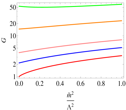
Figure 2: Numerical plot of nontrivial solutions to the soft mass gap equation. Coupling parameter $G$ is plotted against the normalized soft mass parameter $s\;\left(=\frac{\tilde{m}^{2}}{\Lambda^{2}}\right)$ for $t\;\left(=\frac{{|m|}^{2}}{\Lambda^{2}}\right)$ values of $0$ (red), $0.1$ (blue), $0.2$ (pink), $0.4$ (orange), $0.5$ (green), from the lowest to the highest curves, respectively. Notice that the critical coupling increases from $G=1$ for nonzero values of the input supersymmetric mass $m$.

 

$$\tilde{m}^{2}={g^{2}}I(m^{2},\tilde{m}^{2},\Lambda^{2})\;,$$ (5)

where

$$I(m^{2},\tilde{m}^{2},\Lambda^{2}) = \int^{\scriptscriptstyle E}\frac{d^{4}k}{(2\pi)^{4}}\frac{\tilde{m}^{2}(k^{2}-m^{2})}{(k^{2}+m^{2})(k^{2}+m^{2}+\tilde{m}^{2})}$$ (6)

$$= \frac{1}{16\pi^{2}}\left[\Lambda^{2}\tilde{m}^{2}+2m^{4}\ln{\frac{\Lambda^{2}+m^{2}}{m^{2}}}\right.$$

$$\left.\hskip 50.58878pt-(2m^{4}+3m^{2}\tilde{m}^{2}+\tilde{m}^{4})\ln{\frac{(\Lambda^{2}+m^{2}+\tilde{m}^{2})}{(m^{2}+\tilde{m}^{2})}}\right]\;,$$

in which the (Euclidean) momentum loop integral is evaluated with the cut-off $\Lambda$. To check for nontrivial solution, we re-write the equation in dimensionless variables normalized to $\Lambda$

$$\frac{1}{G}=1+\frac{2t^{2}}{s}\ln\left[1+\frac{1}{t}\right]-\left(\frac{2t^{2}}{s}+3t+s\right)\ln\left[1+\frac{1}{t+s}\right]$$ (7)

where $G=\frac{g^{2}\Lambda^{2}}{16\pi^{2}}$, $s=\frac{\tilde{m}^{2}}{\Lambda^{2}}$, and $t=\frac{m^{2}}{\Lambda^{2}}$. Nontrivial solution for the soft mass ($0<s<1$) can be resulted for a large enough coupling, as illustrated numerically in Fig. 2.

It is interesting to note that at the $m=0$ limit, the gap equation reduces to the condition that the momentum integral of the Feynman propagator $\Delta_{\!\scriptscriptstyle F}(k^{2},\tilde{m}^{2})$ equals $\frac{1}{g^{2}}$ or

$$g^{2}\int^{\scriptscriptstyle E}{\Delta_{\!\scriptscriptstyle F}}(k^{2},\tilde{m}^{2})=1\;,$$ (8)

which is the same as the basic NJL model one except with the soft mass $\tilde{m}^{2}$ replacing the (Dirac) fermionic mass (see for example Ref.BE ) if we take $\frac{g^{2}}{2}$ as the four-fermion coupling in the model. This is the $t=0$ case, with critical coupling $G=1$. Nontrivial solution requires bigger and bigger critical coupling as the $m$ increases, and become impossible beyond a limit. Obviously, a $N$ factor is to be multiplied to $g^{2}$ in the gap equation if $\Phi$ is a $N$-multiplet, or $G$ taken as $\frac{Ng^{2}\Lambda^{2}}{16\pi^{2}}$.

III Component Field and Effective Theory Picture

Let us take a look at the component field picture of the model, expanding $\Phi$ as $A+\sqrt{2}\theta\psi+\theta^{2}F$. For simplicity, we drop any reference of a nontrivial ‘color’ factor in the analysis below and pretend that $\Phi$ is just a single superfield. The Lagrangian is given by

$${\cal L} = i\partial_{\mu}\bar{\psi}\bar{\sigma}^{\mu}\psi+\partial^{\mu}A^{*}\partial_{\mu}A+F^{*}F\,+\left(mAF-\frac{m}{2}\psi\psi+h.c.\right)-\frac{g^{2}}{2}|2FA-\psi\psi|^{2}$$ (9)

$$+2g^{2}A^{*}A\,\partial^{\mu}A^{*}\partial_{\mu}A-2g^{2}i\partial_{\mu}\bar{\psi}\bar{\sigma}^{\mu}\psi A^{*}A-2g^{2}i\bar{\psi}\bar{\sigma}^{\mu}\psi A\partial_{\mu}A^{*}\,.$$

Notice that the model has a $U(1)_{\scriptscriptstyle R}$ symmetry under which $A$ and $F$ have charge $+1$ and $-1$. If $m=0$, there will also be a $U(1)$ $\Phi$-number symmetry. From the equation of motion for the auxiliary field $F^{*}$, we have

$$F=-\frac{(m^{*}+g^{2}\psi\psi)A^{*}}{1-2g^{2}|A|^{2}}\;.$$ (10)

The somewhat complicated fractional form of $F$ means that the component field Lagrangian with $F$ eliminated would have less than conventional interaction terms. Naively, the scalar potential is given by

$$-V_{s}=F^{*}F-2g^{2}A^{*}AF^{*}F+mAF+m^{*}A^{*}F^{*}\;.$$ (11)

Eliminating $F$ gives, however,

$$V_{s}=\frac{(|m|^{2}-g^{4}\psi\psi\bar{\psi}\bar{\psi})|A|^{2}}{1-2g^{2}|A|^{2}}\;$$ (12)

which formally no longer involves only the scalar. It is suggestive of a bifermion condensate which fits in the general picture of the NJL setting. It is interesting to note that for $m=0$ the model actually has no pure scalar part in $V_{s}$, for any coupling $g^{2}$. On the other hand, if one neglects the fermion field part in the above, the potential looks simple enough, $V_{s}=\frac{|m|^{2}|A|^{2}}{1-2g^{2}|A|^{2}}$, with a supersymmetric minimum at zero $A$. For positive $g^{2}$, however, it blows up at $|A|=1/\sqrt{2}g$. For a perturbative coupling, one expect $1/g$ bigger than the model cut-off scale $\Lambda$, hence the potential is well behaved within the cut-off. With strong coupling $g^{2}$, one cannot be so comfortable. In fact, for $|A|>1/\sqrt{2}g$, the potential goes negative, contradicting our expectation for a supersymmetric model. The analysis so far suggests compatibility with the superfield gap equation results. Let us go on with the introduction of the effective theory having the composite.

Assuming we do have the composite formation as indicated by the superfield gap equation, the model can also be appreciated with the following effective theory picture, again along the line of NJL-type models. We use parameters $m_{o}$ and $g_{o}$ in the place of $m$ and $g$ in the original Lagrangian to which we add

$$\mathcal{L}_{s}=\int d^{4}\,\theta\frac{1}{2}(\mu U+g_{o}\bar{\Phi}\Phi)^{2}\;,$$ (13)

where $U$ is an ‘auxiliary’ real superfield and mass parameter $\mu$ taken as real and positive (for $g_{o}^{2}>0$). The equation of motion for $U$, from the full Lagrangian $\mathcal{L}+\mathcal{L}_{s}$ gives

$$U=-\frac{g_{o}}{\mu}\bar{\Phi}\Phi\;,$$ (14)

showing it as a superfield composite of $\bar{\Phi}$ and $\Phi$. The condition says the model with $\mathcal{L}+\mathcal{L}_{s}$ is equivalent to that of $\mathcal{L}$ alone. Expanding the term in $\mathcal{L}_{s}$, we have a cancellation of the dimension six interaction in the full Lagrangian, giving it as

$$\mathcal{L}_{ef\!f}\equiv\mathcal{L}+\mathcal{L}_{s}=\int d^{4}\theta\left[\bar{\Phi}\Phi+\frac{\mu^{2}}{2}U^{2}+\mu g_{o}U\bar{\Phi}\Phi+\frac{m_{o}}{2}\Phi^{2}\delta(\bar{\theta})+\frac{m_{o}^{*}}{2}\bar{\Phi}^{2}\delta(\theta)\right]\;.$$ (15)

Obviously, if $\left.U\right|_{D}$ develops a vacuum expectation value (VEV), supersymmetry is broken spontaneously and the superfield $\Phi$ gains a soft supersymmetry breaking mass of $-\mu g_{o}\left\langle\left.U\right|_{D}\right\rangle$. The above looks very much like the standard features of NJL-type model. Notice that while $U$ does contain a vector component, its couplings differ from that of the usually studied ‘vector superfield’ which is a gauge field supermultiplet. That is in addition to having $\mu$ as like a supersymmetric mass for $U$, which can be compatible only with a broken gauge symmetry. As such, model with superfield $U$ is not usually discussed. The superfield can be seen as two parts, as illustrated by the following component expansion,

$$U(x,\theta,\bar{\theta}) = \frac{C(x)}{\mu}+\sqrt{2}\theta\frac{\chi(x)}{\mu}+\sqrt{2}\bar{\theta}\frac{\bar{\chi}(x)}{\mu}+\theta\theta\frac{N(x)}{\mu}+\bar{\theta}\bar{\theta}\frac{{N^{*}}(x)}{\mu}$$ (16)

$$\;\;\;+\sqrt{2}\theta\sigma^{\mu}\bar{\theta}v_{\mu}(x)+\sqrt{2}\theta\theta\bar{\theta}\bar{\lambda}(x)+\sqrt{2}\bar{\theta}\bar{\theta}\theta\lambda(x)+\theta\theta\bar{\theta}\bar{\theta}D(x)\;,$$

where the components $C$, $\chi$, and $N$ is the first part which has the content of like a chiral superfield with however $C$ being real. The $\mu$ factor is put to set the mass dimensions right. The rest is like the content of a superfield for the usual gauge field supermultiplet, with $D$ and $v_{\mu}$ real. Note that $N$, $\chi$ and $\lambda$ carry $U(1)_{\scriptscriptstyle R}$ charges -2, -1 and +1, respectively. The effective Lagrangian in component form is given by

$${\cal L}_{ef\!f} = (1+g_{o}C)\left[A^{*}\Box A+i(\partial_{\mu}\bar{\psi})\bar{\sigma}^{\mu}\psi+F^{*}F\right]+\frac{m_{o}}{2}\left(2AF-\psi\psi\right)+\frac{m^{*}_{o}}{2}\left(2A^{*}F^{*}-\bar{\psi}\bar{\psi}\right)$$ (17)

$$+{\mu}CD-{\mu}\chi\lambda-{\mu}\bar{\chi}\bar{\lambda}+NN^{*}-\frac{\mu^{2}}{2}v^{\nu}v_{\nu}-\mu g_{o}\psi\lambda A^{*}-\mu g_{o}\bar{\psi}\bar{\lambda}A+\mu g_{o}DA^{*}A$$

$$-i\frac{g_{o}}{2}\bar{\psi}\bar{\sigma}^{\mu}\chi\partial_{\mu}A+i\frac{g_{o}}{2}(\partial_{\mu}\bar{\psi})\bar{\sigma}^{\mu}\chi A-g_{o}\chi\psi F^{*}+g_{o}NAF^{*}$$

$$+i\frac{g_{o}}{2}\bar{\chi}\bar{\sigma}^{\mu}\psi\partial_{\mu}A^{*}-i\frac{g_{o}}{2}A^{*}\bar{\chi}\bar{\sigma}^{\mu}\partial_{\mu}\psi-g_{o}\bar{\chi}\bar{\psi}F+g_{o}N^{*}A^{*}F$$

$$-\frac{\mu g_{o}}{\sqrt{2}}\eta^{\mu\nu}v_{\mu}iA^{*}\partial_{\nu}A+\frac{\mu g_{o}}{\sqrt{2}}\eta^{\mu\nu}v_{\mu}i(\partial_{\nu}A^{*})A-\frac{\mu g_{o}}{\sqrt{2}}\eta^{\mu\nu}v_{\mu}\bar{\psi}\bar{\sigma}_{\nu}\psi\;.$$

Notice that $F$, $N$, and $D$ are usual auxiliary components.

In accordance with the ‘quark-loop’ approximation in the (standard) NJL gap equation analysis and our particular supergraph calculation scheme above in particular, we consider plausible nontrivial vacuum solution with nonzero vacuum expectation values (VEVs) for the composite scalars $C$, $N$, and $D$. An effective potential analysis based on the Weinberg tadpole method W ; M is performed with the effective Lagrangian in component form. Vanishing tadpole conditions can be obtained for the scalar potential $V(C,N,D)$ up to one-loop level. Notice that $\left\langle C\right\rangle$ here corresponds to a superfield wavefunction renormalization term $Z=1+g_{o}\left\langle C\right\rangle$ for $\Phi$ or its components. It is the supersymmetric part of $\left.\Sigma^{({\mbox{\tiny}loop})}_{\Phi\Phi^{\dagger}}(p;\theta^{2},\bar{\theta}^{2})\right|_{\mbox{\tiny on-shell}}$, an unavoidable part of the one-loop supergraph in our gap equation calculation for the original Lagrangian discussion in the previous section. One can see the solution equation for the $C$-tadpole under the consistent assumption of $\left\langle N\right\rangle=0$ gives exactly the $\tilde{m}^{2}$ gap equation of Eq.(5) for the here renormalized soft mass parameter in terms of the renormalized mass $m$ and coupling $g$. The treatment in the previous section is essentially non-perturbative. It is natural that superfield $\Phi$ and the parameters there correspond to the renormalized quantities in the present perturbative treatment. The feature will be illustrated more clearly in the next section. We skip all details here. Interested readers are refer to the accompanying paper 063 in which the general case of possible nonzero $\left\langle N\right\rangle$ will be presented.

IV Full Superfield Picture

We present here our formulation based on the advocated strategy of putting superfield functionals as taking values like constant supefields admitting supersymmetric breaking parts 042 . The first step is to add to and subtract from the Lagrangian a term with a full superfield parameter containing the soft mass $\tilde{m}^{2}_{o}$. We introduce the generic form of the superfield parameter

$${\mathcal{Y}}=y-\tilde{\eta}_{o}\theta^{2}-\tilde{\eta}^{*}_{o}\bar{\theta}^{2}-\tilde{m}^{2}_{o}\theta^{2}\bar{\theta}^{2}\;.$$ (18)

For simplicity, we assume $\tilde{\eta}_{o}=0$ and drop it from further consideration. The Lagrangian is split as ${\mathcal{L}}={\mathcal{L}}_{o}+{\mathcal{L}}_{int}$ where ${\mathcal{L}}_{o}=\int\bar{\Phi}\Phi(1+{\mathcal{Y}})+\frac{m_{o}}{2}\Phi^{2}\delta^{2}(\bar{\theta})+\frac{m_{o}^{*}}{2}\bar{\Phi}^{2}\delta^{2}({\theta})$ and ${\mathcal{L}}_{int}=\int-{\mathcal{Y}}\bar{\Phi}\Phi-\frac{g^{2}_{o}}{2}\bar{\Phi}\Phi\bar{\Phi}\Phi$, in which we have hidden the $d^{4}\theta$ and use $m_{o}$ in place of $m$ and for ${g^{2}_{o}}$ in place of $g^{2}$. Obviously, a nonzero $y$ contributes to wavefunction renormalization $\Phi_{\!\scriptscriptstyle R}\equiv\sqrt{Z}\Phi=\sqrt{1+y}\,\Phi$. The quantum effective action is given by

$$\Gamma = \int\bar{\Phi}_{\!\scriptscriptstyle R}\Phi_{\!\scriptscriptstyle R}(1-\tilde{m}^{2}\theta^{2}\bar{\theta}^{2})+\frac{m}{2}\Phi^{2}_{\!\scriptscriptstyle R}\delta^{2}(\bar{\theta})+\frac{m^{*}}{2}\bar{\Phi}^{2}_{\!\scriptscriptstyle R}\delta^{2}({\theta})$$ (19)

$$\hskip 14.45377pt-\frac{\mathcal{Y}}{Z}\bar{\Phi}_{\!\scriptscriptstyle R}\Phi_{\!\scriptscriptstyle R}-\frac{g^{2}}{2}\bar{\Phi}_{\!\scriptscriptstyle R}\Phi_{\!\scriptscriptstyle R}\bar{\Phi}_{\!\scriptscriptstyle R}\Phi_{\!\scriptscriptstyle R}+\Sigma_{\Phi_{\!\scriptscriptstyle R}\Phi_{\!\scriptscriptstyle R}^{\dagger}}\bar{\Phi}_{\!\scriptscriptstyle R}\Phi_{\!\scriptscriptstyle R}+\cdots\;,$$

with now renormalized $m$ and $g^{2}$. The superfield gap equation under the NJL framework is given by

$$-{\mathcal{Y}}_{\!\scriptscriptstyle R}+\left.\Sigma_{\Phi_{\!\scriptscriptstyle R}\Phi_{\!\scriptscriptstyle R}^{\dagger}}^{\tiny(loop)}(p;\theta^{2}\bar{\theta}^{2})\right|_{\mbox{\tiny on-shell}}=0\;,$$ (20)

where ${\mathcal{Y}}_{\!\scriptscriptstyle R}\equiv\frac{\mathcal{Y}}{Z}$. We introduce the expansion $\Sigma_{\Phi_{\!\scriptscriptstyle R}\Phi_{\!\scriptscriptstyle R}^{\dagger}}(p;\theta^{2}\bar{\theta}^{2})=\Sigma_{r}(p)-\Sigma_{\tilde{\eta}}(p)\theta^{2}-\bar{\Sigma}_{\tilde{\eta}^{*}}(p)\bar{\theta}^{2}-\Sigma_{\tilde{m}}(p)\theta^{2}\bar{\theta}^{2}$ from which we can obtain the gap equation for $\tilde{m}^{2}$ as Eq.(5) above. Notice that the standard gap equation picture has to be interpreted here in terms of renormalized superfield and couplings, which is to be expected in the presence of nonzero wavefunction renormalization. The other parts of the superfield gap equation read $\left.\Sigma_{\tilde{\eta}}^{\tiny(loop)}(p)\right|_{\mbox{\tiny on-shell}}=0$ (or rather $=\tilde{\eta}$) and $\left.\Sigma_{r}^{\tiny(loop)}(p)\right|_{\mbox{\tiny on-shell}}=\frac{y}{1+y}$.

It is interesting to see that the effective potential analysis for (the components of) the composite superfield $U$ can be shown directly to be equivalent to the superfield gap equation. Potential minimum condition is given by

$$\mu^{2}\left\langle U\right\rangle+U_{tadpole}=0\qquad\Longrightarrow\qquad\mu g\left\langle U\right\rangle=-g^{2}I^{\tiny(loop)}_{\Phi_{\!\scriptscriptstyle R}\Phi_{\!\scriptscriptstyle R}^{\dagger}}$$ (21)

where $I^{\tiny(loop)}_{\Phi_{\!\scriptscriptstyle R}\Phi_{\!\scriptscriptstyle R}^{\dagger}}$ is the momentum integral of the ${\Phi_{\!\scriptscriptstyle R}\Phi_{\!\scriptscriptstyle R}^{\dagger}}$ propagator loop. Note that from the original Lagrangian with two-superfield composite assumed, we can obtain $-g^{2}\left\langle\left(\Phi_{\!\scriptscriptstyle R}\Phi_{\!\scriptscriptstyle R}^{\dagger}\right)\right\rangle={{\mathcal{Y}}_{\!\scriptscriptstyle R}}$, which is equivalent to $\mu g\left\langle U\right\rangle={{\mathcal{Y}}_{\!\scriptscriptstyle R}}=\left.\Sigma_{\Phi_{\!\scriptscriptstyle R}\Phi_{\!\scriptscriptstyle R}^{\dagger}}^{\tiny(loop)}(p;\theta^{2}\bar{\theta}^{2})\right|_{\mbox{\tiny on-shell}}=-g^{2}I^{\tiny(loop)}_{\Phi_{\!\scriptscriptstyle R}\Phi_{\!\scriptscriptstyle R}^{\dagger}}$. The same loop integral is of course involved in both the gap equation picture and the effective potential analysis. The results here are in direct matching with the correspondent discussion for the NJL case presented in Ref.BE , though for a superfield theory instead. The $\tilde{\eta}$ parameter is to be matched to the $\left\langle N\right\rangle$ in $\left\langle U\right\rangle$ and $\left\langle N\right\rangle=0$ can be shown to be a consistent solution in the effective potential analysis.

V the Goldstino

With the supersymmetry breaking, we expect to have a Goldstino. The required analysis is the ‘quark-loop’ contribution of the two-point function for the composite superfield $U$ in addition to the tree-level mass term. The loop contribution also generates a kinetic term to turn $U$ into a dynamic one. Here in this letter, however, we are contented with a minimal demonstration for a special case. We illustrate here the presence of the Goldstone mode for the special but most interesting case of $m=0$. More details will be left to Ref.063 . We use component field calculation with renormalized $\Phi$ and coupling $g$.

There are two fermionic components of $U$, the $\chi$ and $\lambda$, with the tree-level Dirac mass term $\mu\chi\lambda$. For the $\left\langle N\right\rangle=0$, the $U(1)_{\!\scriptscriptstyle R}$ symmetry is maintained, which protects against any $\chi\chi$ or $\lambda\lambda$ (Majorana) mass term. For $m=0$ then, there is only one diagram contributing to $\lambda\chi$ mass (see Fig. 3). The diagram has a propagator for the scalar $A$ component and one for the fermion $\psi$ component (of the renormalized $\Phi$). The mass produced has a magnitude given by the momentum integral of the two propagators. The diagram has two copies, one has an $A$-momentum, the other a $\bar{\psi}$-momentum dependence at the $\chi$-vertex, with equal and opposite coupling [cf. Eq.(17)]. At zero external momentum, the two copies give equal contributions which add up to a mass term of value to be given by $-2\cdot g\cdot\frac{\mu g}{2}\int^{\scriptscriptstyle E}\Delta_{\!\scriptscriptstyle F}(k^{2},\tilde{m}^{2})$, where $\Delta_{\!\scriptscriptstyle F}(k^{2},\tilde{m}^{2})$ is just the $A$-propagator; the $\psi$-propagator gives only momentum factor(s) that cancels those from the $\chi$-vertex. From the gap equation as given in Eq.(8) one can see that the loop generated mass is exactly $-\mu$, which is equal and opposite to the tree-level mass. So, as the loop tadpoles cancel the tree-level ones generating the symmetry breaking solution, an effectively local term from the loop generated two-field proper vertex cancel the tree-level mass term. The latter is again a generic feature of NJL models, which should work for the full superfield $U$ in our case. For the fermionic components, there is no other piece of contribution to $\chi$ or $\lambda$ masses, hence they are the Goldstino(s). Note that there are wavefunction renormalization terms for $\chi$ and $\lambda$ which make them dynamic. The wavefunction renormalizations do not affect our mass discussion here. The mass for the un-renormalized $\chi$-$\lambda$ sector is zero. The renormalized mass would remain zero.

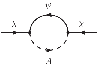
Figure 3: Diagram for $\lambda\chi$ mass.

 

VI Remarks and Conclusions

From our superfield model Lagrangian of Eq.(3), the interaction term $\frac{-g^{2}}{2}\left(\Phi^{\dagger}\Phi\right)\left(\Phi^{\dagger}\Phi\right)$ contains component field parts in the form of kinetic terms multiplied to the scalar field product $A^{*}A$, which may look very un-conventional. However, superfields are scalars on the superspace. The interaction is like a superspace version of four-scalar interaction. It is of dimension six, but quite natural to be considered in models with a cut-off. As a term in the superfield Kahlër potential, the interaction term does not look any stranger than the term $\frac{g^{2}}{2}\left(\Phi^{\dagger}\Phi^{\dagger}\right)\left(\Phi\Phi\right)$, studied before in the first supersymmetric version of the NJL model BL ; BE , which contains the usual NJL four-fermion interaction. The difference is only in the (color) index contraction. On the other hand, in the literature on the original of soft supersymmetry breaking masses for the SSM, similar interaction of the form $-g^{2}_{s}\Phi_{s}^{\dagger}\Phi_{s}\Phi^{\dagger}\Phi$, where $\Phi_{s}$ is the so-called spurion superfield bearing a supersymmetry breaking VEV to communicate supersymmetry breaking to the SSM superfields $\Phi$ has been discussed a lot. Our model can be considered like a similar scenario, only with the $\left\langle\left.\Phi_{s}^{\dagger}\Phi_{s}\right|_{D}\right\rangle$ coming from the dynamically induced two-superfield condensate instead of individual $\left\langle\left.\Phi_{s}\right|_{F}\right\rangle$. But then the kind of $g^{2}_{s}$ term in itself can be the very source of supersymmetry breaking and no extra supersymmetry breaking sector modeling is needed. That should be a very interesting scenario for phenomenological model building. It may even be possible to have a kind of simpler models with the role of $\Phi_{s}$ played by one of the SSM matter superfields themselves. As an initiate nonzero supersymmetric mass for $\Phi_{s}$ is not necessary for the supersymmetry breaking mechanism to work, the chiral nature of the SSM quark superfields does not present a problem. In fact, the $m=0$ is definitely more interesting as it generates mass(es) from no imput mass scale, like the basic NJL model.

Together with the HSNJL model mechanism 034 ; 042 , it is then plausible to have a SSM with no input mass parameter for which soft supersymmetry breaking and a subsequent electroweak symmetry breaking all being generated dynamically within the model. The Higgs superfields are also dynamical composites 034 ; 042 . All one has to do is to consider higher dimensional operators of various four-superfield interaction terms with some having strong couplings. A first soft breaking of supersymmetry as illustrated here can generate the soft masses. Nonzero soft squark masses together with appropriate holomorphic four superfield interaction(s) may induce dynamical electroweak symmetry breaking and generates the masses for the quarks, leptons, and gauge bosons. No other supersymmetry breaking sector, messenger sector, or hidden sector is needed. It is a very simple model without any hierarchy issue. All mass scales are generated dynamically. Such a beautiful scenario of the origin of a phenomenological softly broken SSM will be an interesting target for further studies.

Supersymmetry is a spacetime symmetry. Any theory with rigid supersymmetry could be, and arguably should be, incorporated into a theory with supergravity. In the latter case, the massless Goldstino will be eaten up by the now massive gravitino. The model then should have special implications for the couplings of the longitudinal part of the gravitino to the matter superfields.

The central feature that distinguishes the model from other models of supersymmetry breaking is of course the presence of the spin one composite $v_{\mu}$ and its supersymmetric partners.

We take only the case of a simple singlet composite of $U\sim\Phi^{\dagger}_{a}\Phi^{a}$ here. A somewhat more complicated case as studied in the case of (non-supersymmetric) NJL-type composite of spin one field S would have the composite in the adjoint representation. Similar but superfield version of four-superfield interactions may be considered though not in relation to pure soft supersymmetry breaking. It is also possible to have a model in which the composite superfield $U$ behaves like a massive gauge field supermultiplet 064 , much in parallel with the non-supersymmetric models of Ref.S . It is possible to think about the electroweak gauge bosons as such composites. However, we echo the author of Ref.S against advocating the kind of scenario.

Finally, we emphasize that with the modern effective (field) theory perspective, it is the most natural thing to consider any theory as an effective description of Nature only within a limited domain/scale. Physics is arguably only about effective theories, as any theory can only be verified experimentally up to a finite scale and there may always be a cut-off beyond that. Having a cutoff scale with the so-called nonrenormalizable higher dimensional operators is hence in no sense an undesirable feature. Model content not admitting any other parameter with mass dimension in the Lagrangian would be very natural. Dynamical mass generation with symmetry breaking is then necessary to give the usual kind of low energy phenomenology such as the Standard Model one.

The bottom line is, with relevancy for the supersymmetric standard model or not, we present here a real simple model for dynamical supersymmetry breaking, characterized by the generation of soft mass(es) and a spin one composite.

- (1) Y. Nambu and G. Jona-Lasinio, Phys. Rev. 122, 345 (1961); ibid. 124, 246 (1961).
- (2) G. Faisel, D. W. Jung, and O. C. W. Kong, JHEP 1201, 164 (2012).
- (3) W. Buchmuller and S. T. Love, Nucl. Phys. B 204, 213 (1982).
- (4) W. Buchmuller and U. Ellwanger, Nucl. Phys. B 245, 237 (1984).
- (5) D. W. Jung, O. C. W. Kong and J. S. Lee, Phys. Rev. D 81, 031701 (2010).
- (6) For a review, see Y. Shadmi and Y. Shirman, Rev. Mod. Phys. 72, 25 (2000).
- (7) See for example D.J.H. Chung, L.L. Everett, G.L. Kane, S.F. King, J. Lykken, and L.-T. Wang, Phys. Rep. 407, 1 (2005).
- (8) Y. Cheng, Y.-M. Dai, G. Faisel, and O. C. W. Kong, NCU-HEP-k063, manuscript in preparation.
- (9) W.A. Bardeen, C.N. Leung, and S.T. Love, Phys. Rev. Lett. 56, 1230 (1986); Nucl. Phys. B 273, 649 (1986); ibid. B 323, 493 (1989).
- (10) Y.-M. Dai, G. Faisel, D. W. Jung, and O. C. W. Kong, Phys. Rev. D 87, 085033 (2013).
- (11) S. Weinberg, Phys. Rev. D 7, 2887 (1973) .
- (12) R. D. C. Miller, Phys. Lett. 124B, 59 (1983); Nucl. Phys. B 228, 316 (1983).
- (13) M. Suzuki, Phys. Rev. D 37, 210 (1988); ibid. D 82, 045026 (2010).
- (14) O.C.W. Kong, NCU-HEP-k064, invited talk presented at the XS 2015 conference, July 6-8, Hong Kong. A brief report of results in this letter also presented.