Non-characteristic expansions
of Legendrian singularities

Abstract.

This paper presents an algorithm to deform any Legendrian singularity to a nearby Legendrian subvariety with singularities of a simple combinatorial nature. Furthermore, the category of microlocal sheaves on the original Legendrian singularity is equivalent to that on the nearby Legendrian subvariety. This yields a concrete combinatorial model for microlocal sheaves, as well as an elementary method for calculating them.

1. Introduction

This paper presents an algorithm to deform any Legendrian singularity to a nearby Legendrian subvariety with singularities of a simple combinatorial nature. Furthermore, the category of microlocal sheaves, as developed by Kashiwara-Schapira [13], on the original Legendrian singularity is equivalent to that on the nearby Legendrian subvariety. This yields a concrete combinatorial model for microlocal sheaves, in terms of modules over quivers, as well as an elementary method for calculating them.

Among other applications, it allows one to establish new homological mirror symmetry equivalences for Landau-Ginzburg models with singular thimbles [21]. It also provides a key tool in the foundations of microlocal sheaves, in particular in the recent development of its wrapped variant [23]. Furtheremore, it underlies ongoing work on the structure of Weinstein manifolds [6] and their Fukaya categories [8].

In the rest of the introduction, we first state the main results of the paper, then sketch some of the arguments involved in their proof. Finally, we elaborate further on their place in the subject, in particular their original motivation in conjectures of Kontsevich [16] and a program of MacPherson and collaborators (see for example [4, 9]) devoted to combinatorial models of respectively Fukaya categories and microlocal sheaves.

1.1. Main results

A natural setting for the paper is local contact geometry. (See Sects. 2 and 3 below for detailed geometric preliminaries.)

Let $M$ be a smooth manifold with cotangent bundle $T^{*}M$ with its canonical exact symplectic structure. Introduce the cosphere bundle

with its canonical cooriented contact structure. By the contact Darboux theorem, any contact manifold is locally equivalent to $S^{*}M$.

By a Legendrian subvariety $\Lambda\subset S^{*}M$, we will mean a closed Whitney stratified subspace of pure dimension $\dim\Lambda=\dim M-1$ whose strata are isotropic for the contact structure. By a Legendrian singularity $\Lambda\subset S^{*}M$ , we will mean the germ of a Legendrian subvariety at a point $z\in\Lambda$ which we refer to as its center.

We will assume that any Legendrian singularity $\Lambda\subset S^{*}M$ we encounter can be placed in generic position in the sense that the front projection $H=\pi(\Lambda)\subset M$ is the germ at the image of the center $x=\pi(z)$ of a Whitney stratified hypersurface, and the restriction

is a finite map. (To simplify the exposition, we will also assume the Whitney stratification of $H$ satisfies some modest local connectivity which can always be arranged by refining the stratification, see Sect. 5.1 for details).

Fix a field $k$, and following Kashiwara-Schapira [13] (and reviewed in Sect. 6 below) given a Legendrian subvariety $\Lambda\subset S^{*}M$, introduce the dg category $\mu\mathit{Sh}_{\Lambda}(S^{*}M)$ of constructible microlocal complexes of $k$-modules on $S^{*}M$ supported along $\Lambda$. (The results and arguments of the paper work equally well without the constructible hypothesis, but we include it to keep within a traditional setting.) In particular, for a Legendrian singularity $\Lambda\subset S^{*}M$ in generic position, and a small open ball $B\subset M$ around the image of the center $x=\pi(z)$, there is a canonical quotient presentation

in terms of the more concrete dg category $\mathit{Sh}_{\Lambda}(B)$ of constructible complexes on $B$ with singular support in $\Lambda$, and its full dg subcategory ${\mathcal{L}oc}(B)$ of finite-rank derived local systems.

In the paper [20], we introduced a natural class of Legendrian singularities $\Lambda_{\mathcal{T}}\subset S^{*}{\mathbb{R}}^{|\mathcal{T}|}$, called arboreal singularities, indexed by rooted trees $\mathcal{T}$ (finite connected acyclic graphs with a choice of root vertex), where $|\mathcal{T}|$ denotes the number of vertices of the underlying tree. Each is naturally stratified by strata $\Lambda_{\mathcal{T}}(\mathfrak{p})\subset\Lambda_{\mathcal{T}}$ indexed by correspondences of trees

with $i$ an inclusion of a full subtree, and $q$ a quotient by collapsing edges. Moreover, the normal geometry to the stratum $\Lambda_{\mathcal{T}}(\mathfrak{p})\subset\Lambda_{\mathcal{T}}$ is equivalent via Hamiltonian reduction to the arboreal singularity $\Lambda_{\mathcal{R}}\subset S^{*}{\mathbb{R}}^{|{\mathcal{R}}|}$.

Passing to microlocal sheaves, we constructed in [20] a canonical equivalence

where $\operatorname{Perf}(\mathcal{T})$ denotes the dg category of perfect complexes over the quiver associated to the rooted tree $\mathcal{T}$ where all edges are directed away from the root vertex. We also showed that for each stratum $\Lambda_{\mathcal{T}}(\mathfrak{p})\subset\Lambda_{\mathcal{T}}$, the corresponding microlocal restriction functor

is given by the integral transform

where $i^{*}$ kills the projective object $P_{\alpha}\in\operatorname{Perf}(\mathcal{T})$ attached to $\alpha\in\mathcal{T}\setminus{\mathcal{S}}$, and and $q_{!}$ identifies the projective objects $P_{\alpha},P_{\beta}\in\operatorname{Perf}({\mathcal{S}})$ attached to $\alpha,\beta\in{\mathcal{S}}$ such that $q(\alpha)=q(\beta)\in{\mathcal{R}}$.

In Sect. 4 below, we review the basic properties of arboreal singularities, and introduce natural generalizations $\Lambda_{\mathcal{T}^{*}}\subset S^{*}{\mathbb{R}}^{|\mathcal{T}^{*}|}$ indexed by leafy rooted trees $\mathcal{T}^{*}$ (finite connected acyclic graphs with a choice of root vertex and a subset of leaf vertices), where $|\mathcal{T}^{*}|$ denotes the sum of the number of vertices of the underlying tree and the number of marked leaves. Similar statements to those recalled above hold for generalized arboreal singularities.

By an arboreal Legendrian subvariety $\Lambda\subset S^{*}M$, we will mean a Legendrian subvariety such that its normal geometry along each of its strata is equivalent via Hamiltonian reduction to an arboreal singularity $\Lambda_{\mathcal{T}^{*}}\subset S^{*}{\mathbb{R}}^{|\mathcal{T}^{*}|}$. Thus for an arboreal Legendrian subvariety $\Lambda\subset S^{*}M$, the dg category of microlocal sheaves $\mu\mathit{Sh}_{\Lambda}(S^{*}M)$ admits an elementary description: it is the global sections of a sheaf of dg categories over $\Lambda\subset S^{*}M$ that assigns perfect modules over trees to small open sets, integral transforms for correspondences of trees to inclusions of small open sets, along with natural higher coherences.

Now to state the main result of this paper, we need one further key concept.

By a deformation of a Legendrian singularity $\Lambda\subset S^{*}M$ to a Legendrian subvariety $\Lambda^{\prime}\subset S^{*}M$, we will mean a Legendrian subvariety $\tilde{\Lambda}\subset S^{*}(M\times{\mathbb{R}})$ supported over the parameters ${\mathbb{R}}_{\geq 0}$ with special Hamiltonian reduction $\tilde{\Lambda}_{0}=\Lambda\subset S^{*}M$ the original Legendrian singularity, and generic Hamiltonian reductions $\tilde{\Lambda}_{t}\simeq\Lambda^{\prime}\subset S^{*}M$ all equivalent for $t>0$.

It is not true in general that microlocal sheaves will be constant under such deformations, even if we insist on strong topological properties. (See Example 1.5 below.) By a non-characteristic deformation, we will mean one for which Hamiltonian reduction at any of the parameters ${\mathbb{R}}_{\geq 0}$ induces an equivalence on microlocal sheaves.

Theorem 1.1.

Let $\Lambda\subset S^{*}M$ be a Legendrian singularity.

The expansion algorithm of Sect. 5 provides a non-characteristic deformation of $\Lambda\subset S^{*}M$ to an arboreal Legendrian subvariety $\Lambda_{\mathit{arb}}\subset S^{*}M$.

Our use of the term expansion reflects the idea that we perform a kind of “spherical real blowup” to expand complicated singularities into irreducible components which then interact in a combinatorial way. One could compare this with resolutions of singularities in algebraic geometry where complicated singularities become divisors with normal crossings. Proving the expansion algorithm is non-characteristic occupies Sect. 6 below and is the most technically involved part of the paper.

Remark 1.2.

One can easily refine the expansion algorithm so that $\Lambda_{\mathit{arb}}\subset S^{*}M$ is as $C^{0}$-close to $\Lambda\subset S^{*}M$ as one wishes.

Corollary 1.3.

Let $\Lambda\subset S^{*}M$ be a Legendrian singularity.

There is a canonical equivalence between the dg category $\mu\mathit{Sh}_{\Lambda}(S^{*}M)$ of microlocal sheaves and the global sections of a sheaf of dg categories over $\Lambda_{\mathit{arb}}\subset S^{*}M$ that assigns perfect modules over trees to small open sets, integral transforms for correspondences of trees to inclusions of small open sets, along with natural higher coherences.

One can view the theorem and corollary as providing analogies with basic results of Morse theory.

On the one hand, any germ of a smooth function $f:M\to\mathbb{R}$ can be deformed to a nearby function with Morse singularities. Moreover, Morse singularities are of a simple combinatorial form enumerated by their Morse index $0\leq k\leq\dim M$. What results is a combinatorial description of the cohomology of $M$ in terms of the the Morse-Witten complex.

On the other hand, any Legendrian singularity $\Lambda\subset S^{*}M$ can be deformed to a Legendrian subvariety with arboreal singularities. Moreover, arboreal singularities are of a simple combinatorial form enumerated by leafy rooted trees. What results is a combinatorial description of microlocal sheaves along $\Lambda\subset S^{*}M$ in terms of a diagram of perfect modules over trees.

We have not attempted to formulate here the sense in which arboreal singularities are the “stable” Legendrian singularities, though we expect the analogy to extend in this direction.

Remark 1.4.

We have used the term non-characteristic to mean that the dg category of microlocal sheaves is invariant under the deformation. We expect this to be a consequence of the following more basic geometric notion.

For any choice of Reeb vector field and resulting Reeb flow $\varphi_{t}$, a reasonable Legendrian singularity $\Lambda\subset S^{*}M$ will admit a small $\epsilon>0$ so that the Reeb flow displaces

In other words, there will be no positive Reeb trajectories from $\Lambda$ to itself of length less than $\epsilon$.

We expect a deformation $\tilde{\Lambda}\subset S^{*}(M\times{\mathbb{R}})$ will be non-characteristic if there is a small $\epsilon>0$ so that the Reeb flow displaces

In other words, there will be no positive Reeb trajectories from $\tilde{\Lambda}_{s}$ to itself of length less than $\epsilon$ for all parameters $s\in{\mathbb{R}}_{\geq 0}$.

Example 1.5.

Take $M=\mathbb{R}^{2}$ with coordinates $x,y$. Introduce the hypersurface

as pictured in Fig. 1. It is the homeomorphic wavefront projection of a Legendrian subvariety $\Lambda\subset S^{*}\mathbb{R}^{2}$ given by the closure of the restriction of the $dy$ codirection to the conormal of the smooth locus of $H$. As a topological space, the curve $H$, and hence the Legendrian subvariety $\Lambda$, is the union of three real lines all glued to each other at zero to form a six-valent node.

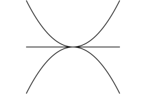
Figure 1. Front projection of initial Legendrian $\Lambda\subset S^{*}{\mathbb{R}}^{2}$.

We will describe two deformations of $\Lambda\subset S^{*}M$ to nearby Legendrian subvarieties with simpler singularities, but only the first will be a non-characteristic deformation.

1) For $s\geq 0$, consider the family of hypersurfaces

pictured in Fig. 2. It is the homeomorphic wavefront projection of a non-characteristic family of Legendrian subvarieties $\Lambda_{s}\subset S^{*}\mathbb{R}^{2}$ given by the closure of the restriction of the $dy$ codirection to the conormal of the smooth locus of $H_{s}$. When $s>0$, as a topological space, the curve $H_{s}$, and hence the Legendrian subvariety $\Lambda_{s}$, has two singularities which are four-valent nodes.

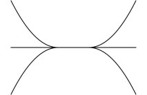
Figure 2. Front projection of non-characteristic deformation.

2) For $s\geq 0$, consider the family of hypersurfaces

pictured in Fig. 3. It is the homeomorphic wavefront projection of a family of Legendrian subvarieties $\Lambda_{s}\subset S^{*}\mathbb{R}^{2}$ given by the closure of the restriction of the $dy$ codirection to the conormal of the smooth locus of $H_{s}$. When $s>0$, as a topological space, the curve $H_{s}$, and hence the Legendrian subvariety $\Lambda_{s}$, has two singularities which are four-valent nodes. But the family is not non-characteristic: for any small $\epsilon>0$, there is a small $s>0$ so that there is a geodesic in ${\mathbb{R}}^{2}$, positive with respect to $dy$, of length less than $\epsilon$, from a point of $\{y+(x+s)^{2}=0\}$ to a point of $\{y-(x-s)^{2}=0\}$ and orthogonal to each.

Figure 3. Front projection of characteristic deformation.

1.2. Sketch of arguments

We briefly sketch here the idea behind the expansion algorithm of Theorem 1.1 in the case of one-dimensional Legendrian singularities. As topological spaces, one-dimensional Legendrian subvarieties are nothing more than graphs, and it is not difficult to understand their deformations. But let us use this special case to give a hint about the proof of the general case which is a somewhat intricate inductive pattern built out of similar arguments.

First, it suffices to take $M=\mathbb{R}^{2}$ with coordinates $x,y$. Any Legendrian singularity $\Lambda\subset S^{*}{\mathbb{R}}^{2}$ in generic position has wavefront projection a singular plane curve $C=\pi(\Lambda)\subset{\mathbb{R}}^{2}$ as pictured in Fig. 4. We may assume $C$ passes through the origin $0\in{\mathbb{R}}^{2}$, is smooth away from $0$, so that $\Lambda$ defines a coorientation of $C\setminus\{0\}\subset{\mathbb{R}}^{2}$, and the fiber at the origin $\Lambda|_{0}\subset S^{*}_{0}{\mathbb{R}}^{2}$ is the single codirection $dy$. With this setup, the wavefront projection from the Legendrian $\Lambda\subset S^{*}{\mathbb{R}}^{2}$ to the curve $C\subset{\mathbb{R}}^{2}$ is a homeomorphism. (A significant complication in higher dimensions is the fact that it is only possible to arrange for the wavefront projection to be a finite map.)

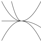
Figure 4. Initial front projection $C\subset{\mathbb{R}}^{2}$.

Next, consider the circle $S(r)\subset{\mathbb{R}}^{2}$ of a small radius $r>0$ around the origin $0\in{\mathbb{R}}^{2}$. Let us assume $S(r^{\prime})$ is transverse to $C$, for all radii $0<r^{\prime}\leq r$. For a very small constant $d>0$, introduce the closed subarc of the circle

Consider the closed ball $B(r)\subset{\mathbb{R}}^{2}$ of radius $r$ around the origin $0\in{\mathbb{R}}^{2}$, and form a new curve given by the union

as pictured in Fig. 5.

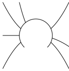
Figure 5. Intermediate curve $C_{\mathit{pre}}\subset{\mathbb{R}}^{2}$.

Observe that $C_{\mathit{pre}}$ is smooth away from the finitely many points of the intersection $C\cap S(r)$. Moreover, away from these points, it has a canonical coorientation given by $\Lambda$ along $C\setminus(C\cap B(r))$, and by the outward radial differential $dr$ along $E\setminus(C\cap S(r))$. Working locally near each of the points of $C\cap S(r)$, we can smooth $C_{\mathit{pre}}\subset{\mathbb{R}}^{2}$ to a new homeomorphic curve $C_{\mathit{arb}}\subset{\mathbb{R}}^{2}$, as pictured in Fig. 6, that has an unambiguous coorientation defined everywhere. Thus there is a corresponding Legendrian $\Lambda_{\mathit{arb}}\subset S^{*}{\mathbb{R}}$ with homeomorphic wavefront projection to $C_{\mathit{arb}}\subset{\mathbb{R}}^{2}$.

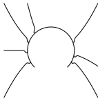
Figure 6. Final curve $C_{\mathit{arb}}\subset{\mathbb{R}}^{2}$.

Finally, the singularities of $C_{\mathit{arb}}$, and hence those of $\Lambda_{\mathit{arb}}$, are of two combinatorial types. First, in a neighborhood of the points of the intersection $C\cap S(r)$, the singularities are trivalent nodes. With the exception of smooth points, these are the simplest example of arboreal singularities. In a neighborhood of the boundary ends of the subarc

we find univalent nodes. These are the simplest example of the generalized arboreal singularities discussed in Sect. 4 below. One might hope to find only trivalent nodes and not univalent nodes, but if the original Legendrian $\Lambda\subset S^{*}{\mathbb{R}}^{2}$, and hence curve $C\subset{\mathbb{R}}^{2}$, itself had a univalent node, it would be awkward to try to deform away a univalent node rather than accept it as a reasonable singularity.

1.3. Motivations

We summarize here some of the prior and ongoing work motivating the results this paper.

To start, there is a well established expectation that the Fukaya category of an exact symplectic manifold, specifically a Weinstein manifold, admits a description in terms of microlocal sheaves supported on a Lagrangian skeleton. (Alternatively, to more closely approach the setting of this paper, one can formulate both theories on the contactification of the exact symplectic manifold along with the Legendrian lift of the skeleton.) There are two primary variants of this expectation: the infinitesimal Fukaya category [7, 26] of compact branes running along the skeleton corresponds to constructible microlocal sheaves, and the wrapped Fukaya category [1] of non-compact branes transverse to the skeleton corresponds to wrapped microlocal sheaves (see [23] for further discussion). It is also possible to formulate a unified version involving non-compact skeleta and the partially wrapped Fukaya category [2]. The expectation can be realized in many settings, notably for cotangent bundles [24, 18].

The Fukaya category and microlocal sheaves each have their advantages and challenges. On the one hand, the Fukaya category is evidently a symplectic invariant, and in particular independent of the choice of a skeleton. Its objects have clear geometric appeal, though its morphisms involves challenging global analysis. On the other hand, microlocal sheaves form a sheaf along the skeleton, and enjoy powerful functoriality developed by Kashiwara-Schapira [13]. Its objects are often quite abstract, and in particular involve choices of local polarizations.

Without a comprehensive theory that the Fukaya category and microlocal sheaves coincide, one is naturally led to the following questions.

First, given a skeleton, is there a sheaf of dg categories whose global sections is the Fukaya category? This was conjectured by Kontsevich [16] and establishing instances of the resulting local-to-global gluing is an active theme in the subject.

Second, is there an elementary way to define and calculate microlocal sheaves along a skeleton? This has been the focus of a longstanding program pioneered by MacPherson (notably for microlocal perverse sheaves in the holomorphic symplectic setting), and advanced for example by Gelfand-MacPherson-Vilonen [9].

The current paper provides an answer to this second question in terms of the linear algebra of modules over quivers. It can be applied to reduce any calculation about microlocal sheaves to a finite amount of linear algebra. This was implemented in [21] to establish a central instance of mirror symmetry where the skeleton is a three-dimensional singular thimble. Namely, a simple application of the expansion algorithm provides the main step in the proof of the following.

Theorem 1.6 ([21]).

Set $M=\mathbb{C}^{3}$ with its conic exact symplectic structure, and $\Lambda\subset M$ the Lagrangian cone over the standard Legendrian torus $T^{2}\subset S^{5}$.

There are are equivalences of dg categories

where $\mu\mathit{Sh}_{\Lambda}(M)$ and $\mu\mathit{Sh}^{w}_{\Lambda}(M)$ denote respectively traditional and wrapped microlocal sheaves on $M$ supported along $\Lambda$, and $\operatorname{Coh}(\mathbb{P}^{1}\setminus\{0,1,\infty\})$ and $\operatorname{Coh}_{\mathit{tors}}(\mathbb{P}^{1}\setminus\{0,1,\infty\})$ denote the dg category of respectively coherent complexes and coherent complexes with proper support on $\mathbb{P}^{1}\setminus\{0,1,\infty\}$.

In another direction, the results of this paper were invoked in [23] to establish that traditional microlocal sheaves and wrapped microlocal sheaves are dual in a sense parallel to the duality of perfect complexes and coherent complexes [3], or more basically, functions/cohomology and distributions/homology. More precisely, it provided the central tool in the proof of the following, reducing the assertion to a simple observation about modules over trees.

Theorem 1.7 ([23]).

Let $\Omega\subset T^{*}X$ be a conic open subset, and $\Lambda\subset T^{*}X$ a closed conic Lagrangian subvariety.

The natural hom-pairing provides an equivalence

where $\mu\mathit{Sh}_{\Lambda}(\Omega)$ and $\mu\mathit{Sh}^{w}_{\Lambda}(\Omega)$ denote respectively traditional and wrapped microlocal sheaves on $\Omega$ supported along $\Lambda$, $\operatorname{Fun}^{ex}$ denotes the dg category of exact functors, and $\operatorname{Perf}_{k}$ denote the dg category of perfect $k$-modules.

At a more fundamental level, the current paper also provides the basis for answering the first question, about sheafifying the Fukaya category along a skeleton, via showing the Fukaya category and microlocal sheaves coincide. Namely, in ongoing work with Eliashberg and Starkston [6], its techniques are applied to show that any Weinstein manifold admits an arboreal skeleton. From here, ongoing work of Ganatra-Pardon-Shende [8] shows that given an arboreal skeleton, the Fukaya category is equivalent to microlocal sheaves along it. Going further, we expect that arboreal skeleta will provide a higher dimensional notion of ribbon graphs from which one can recover the ambient symplectic manifold itself. These developments rest upon the fact that the singularities of skeleta can be deformed to arboreal singularities.

1.4. Summary of sections

Here is a brief summary of the specific contents of the sections of the paper. Sect. 2 summarizes standard material from singularity theory, in particular Whitney stratifications and their control data which provide the language for our geometric constructions. Sect. 3 summarizes the basic structure of wavefront projections in the form of directed hypersurfaces and positive coray bundles. Sect. 4 reviews the notion of arboreal singularities from [20], then extends their exposition to generalized arboreal singularities. Sect. 5 contains our main geometric constructions: it presents the expansion algorithm that takes a Legendrian singularity to an arboreal Legendrian subvariety. Sect. 6 contains our main technical arguments: it proves that the expansion algorithm is non-characteristic in the sense that the dg category of microlocal sheaves is invariant under it. Finally, a brief appendix summarizes the data that goes into the expansion algorithm, in particular the hierarchy of the chosen constants.

1.5. Acknowledgements

I thank D. Auroux, D. Ben-Zvi, M. Goresky, J. Lurie, I. Mirković, N. Rozenblyum, D. Treumann, H. Williams, L. Williams, and E. Zaslow for their interest, encouragement, and valuable comments. I am additionally grateful to D. Treumann for generously creating the pictures appearing in the figures. Finally, I am grateful to the NSF for the support of grant DMS-1502178.

2. Preliminaries

This section collects standard material on stratification theory following Mather [17].

We write $\mathbb{R}$ for the real numbers, $\mathbb{R}_{>0}$ for the positive real numbers, and $\mathbb{R}_{\geq 0}$ for the non-negative real numbers. All manifolds will be smooth and equidimensional and all maps will be smooth unless otherwise stated.

2.1. Whitney stratifications

Let $M$ be an manifold and $X\subset M$ a closed subspace. A Whitney stratification of $X$ is a disjoint decomposition

$$X=\cup_{\alpha\in A}X_{\alpha}$$

into submanifolds $X_{\alpha}\subset M$ satisfying:

(Axiom of the frontier) If $X_{\alpha}\cap\overline{X}_{\beta}\not=\emptyset$, then $X_{\alpha}\subset\overline{X}_{\beta}$.

(Local finiteness) Each point $x\in M$ has an open neighborhood $U\subset M$ such that $U\cap X_{\alpha}=\emptyset$ for all but finitely many $\alpha\in A$.

(Whitney’s condition $B$) If sequences $a_{k}\in X_{\alpha}$ and $b_{k}\in X_{\beta}$ converge to some $a\in X_{\alpha}$, and the sequence of secant lines $[a_{k}b_{k}]$ (with respect to a local coordinate system) and tangent planes $T_{b_{k}}X_{\beta}$ both converge, then $\lim_{k}[a_{k}b_{k}]\subset\lim_{k}TX_{\beta}$.

The index set $A$ is naturally a poset with $\alpha<\beta$ when $X_{\alpha}\not=X_{\beta}$ and $X_{\alpha}\subset\overline{X}_{\beta}$.

We will say that $X$ has dimension $k$ if it is the closure of its strata of dimension $k$.

Remark 2.1.

Note that we can trivially extend any Whitney stratification of $X\subset M$ to a Whitney stratification of all of $M$ by including the open complement $M\setminus X$ itself as a stratum.

Given a Whitney stratification of $X\subset M$, by a small open ball $B\subset M$ around a point $x\in M$, we will always mean an open ball of radius $R>0$ with respect to the Euclidean metric of some local coordinate system. Moreover, we will assume that for any $0<r\leq R$, the sphere around $x$ of radius $r$ is transverse to the strata. Whitney’s condition $B$ guarantees this holds for any local coordinate system and small enough $R>0$.

2.2. Control data

Let $M$ be an manifold.

A tubular neighborhood of a submanifold $Y\subset M$ consists of an inner product on the normal bundle $p:E\to Y$, and a smooth embedding

of the open ball bundle determined by some $\epsilon>0$. The image $T=\varphi(E[{<\epsilon}])$ is required to be an open neighborhood of $Y\subset M$, and the restriction of $\varphi$ to the zero section $Y\subset E$ is required to be the identity map to $Y\subset M$. By rescaling the inner product, we can assume that $\epsilon=1$.

By transport of structure, the neighborhood $T$ comes equipped with the tubular distance function $\rho:T\to\mathbb{R}_{\geq 0}$ and tubular projection $\pi:T\to Y$ defined by

We will write $(T,\rho,\pi)$ to denote the tubular neighborhood and remember that $\pi:T\to Y$ is the open unit ball bundle in a vector bundle with inner product inducing $\rho:T\to\mathbb{R}_{\geq 0}$.

Given small $\epsilon\geq 0$, we have the inclusions

and similarly with $<$ replaced by $\leq,>,$ or $\geq$. Of course when $\epsilon=0$, we have $T[<\epsilon]=\emptyset$, $T[\leq\epsilon]=S[\epsilon]=Y$, $T[>\epsilon]=T\setminus Y$, $T[\geq\epsilon]=T$.

Any Whitney stratified subspace $X\subset M$ admits a compatible system of control data consisting of a tubular neighborhood $(T_{\alpha},\rho_{\alpha},\pi_{\alpha})$ of each stratum $X_{\alpha}\subset X$. Whenever $\alpha<\beta$, the tubular distance functions and tubular projections are required to satisfy

on the common domain of points $x\in T_{\alpha}\cap T_{\beta}$ such that $\pi_{\beta}(x)\in T_{\alpha}$.

A key property of a system of control data is the fact that the product map

has surjective differential when restricted to any stratum $X_{\beta}\subset X$ with $\beta>\alpha$.

2.3. Almost retraction

Let $M$ be a manifold.

Let $X\subset M$ be a closed subspace with Whitney stratification $\{X_{\alpha}\}_{\alpha\in A}$.

Suppose given a compatible system of control data $\{(T_{\alpha},\rho_{\alpha},\pi_{\alpha})\}_{\alpha\in A}$.

Following Goresky [10, 11], we review some further fundamental constructions.

Fix once and for all a small $\epsilon>0$.

Choose a family of lines subordinate to the system of control data. This consists of a retraction

for each $\alpha\in A$ satisfying the following. For $\alpha<\beta$, one requires $r_{\alpha}|_{X_{\beta}}$ is smooth and the compatibilities

on their natural domains. The retractions provide homeomorphisms

and for $B\subset A$, more general collaring homeomorphisms

where $k=|B|$ and the indices $\alpha_{i}\in B$ can be arbitrarily ordered thanks to $r_{\alpha_{i}}r_{\alpha_{j}}=r_{\alpha_{j}}r_{\alpha_{i}}$.

Fix a smooth nondecreasing function $q:\mathbb{R}\to\mathbb{R}$ such that $q(t)=0$, for $t\leq\epsilon$, and $q(t)=t$, for $t\geq 2\epsilon$. For each stratum $X_{\alpha}\subset X$, introduce the mapping

$$\Pi_{\alpha}:M\longrightarrow M\hskip 30.00005pt\Pi_{\alpha}(x)=\left\{\begin{array}[]{cl}x&\mbox{ when }x\not\in T_{\alpha}[<2\epsilon]\\ h^{-1}_{\alpha}(r_{\alpha}(x),q(\rho_{\alpha}(x)))&\mbox{ when }x\in T_{\alpha}[<2\epsilon]\end{array}\right.$$

It is continuous, homotopic to the identity, and satisfies $\Pi_{\alpha}(x)=\pi_{\alpha}(x)$ when $x\in T_{\alpha}[\leq\epsilon]$. Moreover, the mappings commute $\Pi_{\alpha}\Pi_{\beta}=\Pi_{\beta}\Pi_{\alpha}$, for $\alpha,\beta\in A$. To confirm this, if $x\not\in T_{\alpha}[<2\epsilon]$, then $\Pi_{\alpha}(x)=x$, and $\Pi_{\beta}(x)\not\in T_{\alpha}[<2\epsilon]$ since $\rho_{\alpha}r_{\beta}(x)=\rho_{\alpha}(x)$, so $\Pi_{\alpha}\Pi_{\beta}(x)=\Pi_{\beta}(x)=\Pi_{\beta}\Pi_{\alpha}(x)$. If $x\in T_{\alpha}[<2\epsilon]\cap T_{\beta}[<2\epsilon]$, then

Now introduce the composition

where $N+1=|A|$ and the indices $\alpha_{i}\in A$ can be arbitrarily ordered thanks to $\Pi_{\alpha_{i}}\Pi_{\alpha_{j}}=\Pi_{\alpha_{j}}\Pi_{\alpha_{i}}$. It is continuous, homotopic to the identity, and satisfies

The restriction of $r$ to the open subspace

$$U[<\epsilon]=\bigcup_{\alpha\in A}T_{\alpha}[<\epsilon]\subset M$$

is almost a retraction of $U[<\epsilon]$ to $X$ in that it maps $U[<\epsilon]$ to $X$ and the restriction of $r$ to $X$ is homotopic to the identity. In fact, the restriction of $r$ to $X$ is the identity on any $x\in X$ whenever $x\in X_{\alpha}\setminus\cup_{\beta<\alpha}(X_{\alpha}\cap T_{\beta}[<2\epsilon])$ for some $\alpha\in A$.

Remark 2.2.

The above constructions are well suited to inductive arguments. Fix a closed stratum $X_{0}\subset X$, and set $M^{\prime}=M\setminus X_{0}$, $X^{\prime}=X\setminus X_{0}$. The system of control data and family of lines for $X\subset M$ immediately provide the same for $X^{\prime}\subset M^{\prime}$ by deleting the data for $X_{0}\subset X$. The resulting almost retraction $r^{\prime}:M^{\prime}\to M^{\prime}$ satisfies the following evident compatibility with the almost retraction $r:M\to M$. Introduce the composition

so that $r=\Pi_{0}\hat{r}_{0}$. Then $\hat{r}_{0}|_{X_{0}}=\operatorname{id}_{X_{0}}$ and $\hat{r}_{0}|_{M^{\prime}}=r^{\prime}$.

Remark 2.3.

By convention, when $X=\emptyset$, we set $r=\operatorname{id}_{M}:M\to M$ to be the identity. This would naturally result from invoking the above constructions with the complement $M\setminus X\subset M$ itself as a stratum. This is a trivial modification since the tubular neighborhood of such an open stratum is simply itself.

2.4. Multi-transversality

Let $M$ be an manifold.

We say that a finite set ${\mathfrak{F}}=\{f_{i}\}_{i\in I}$ of functions $f_{i}:M\to\mathbb{R}$ is multi-transverse at a value $s_{I}=(s_{i})\in\mathbb{R}^{I}$ if for any subset $J\subset I$, the product map

is a submersion along $F_{J}^{-1}(s_{J})\subset M$ where $s_{J}=(s_{j})\in\mathbb{R}^{J}$ is the image of $s_{I}=(s_{i})\in\mathbb{R}^{I}$ under the natural projection $\pi_{J}:\mathbb{R}^{I}\to\mathbb{R}^{J}$.

If ${\mathfrak{F}}=\{f_{i}\}_{i\in I}$ is multi-transverse at $s_{I}=(s_{i})\in\mathbb{R}^{I}$, then the level-sets

are smooth hypersurfaces (if non-empty) and multi-transverse in the following sense. For any subset $J\subset I$, the intersection

is a smooth submanifold of codimension $|J|$ (if non-empty), and transverse to $H_{i}(s_{i})\subset M$, for each $i\in I\setminus J$.

Suppose a finite set ${\mathfrak{F}}=\{f_{i}\}_{i\in I}$ of functions $f_{i}:M\to\mathbb{R}$ is multi-transverse at a value $s_{I}=(s_{i})\in\mathbb{R}^{I}$. Then given another function $f:M\to\mathbb{R}$ and a value $s\in\mathbb{R}$, we may find a nearby value $s^{\prime}\in\mathbb{R}$ so that the extended set $\{f\}\coprod\{f_{i}\}_{i\in I}$ of functions is multi-transverse at the extended value $(s^{\prime},s_{i})\in\mathbb{R}\times\mathbb{R}^{I}$. This follows from Sard’s Theorem: there is a nearby regular value $s^{\prime}\in\mathbb{R}$ for the function

Thus given any finite set ${\mathfrak{F}}=\{f_{i}\}_{i\in I}$ of functions $f_{i}:M\to\mathbb{R}$ and a value $s=(s_{i})\in\mathbb{R}^{I}$, by induction on any order of $I$, there is a nearby value $s^{\prime}=(s^{\prime}_{i})\in\mathbb{R}^{I}$ such that ${\mathfrak{F}}=\{f_{i}\}_{i\in I}$ is multi-transverse at $s^{\prime}=(s^{\prime}_{i})\in\mathbb{R}^{I}$.

Example 2.4.

(1) Let $M=\mathbb{R}$ with coordinate $x$. Set $f_{1}=f_{2}=x$. Then ${\mathfrak{F}}=\{f_{1},f_{2}\}$ is multi-transverse at $(s_{1},s_{2})\in\mathbb{R}^{2}$ if and only if $s_{1}\not=s_{2}$.

(2) Let $M=\mathbb{R}^{2}$ with coordinates $x_{1},x_{2}$. Set $f_{1}=x_{1}$, $f_{2}=x_{2}$, and $f_{3}=x_{1}+x_{2}$. Then ${\mathfrak{F}}=\{f_{1},f_{2},f_{3}\}$ is multi-transverse at $(s_{1},s_{2},s_{3})\in\mathbb{R}^{3}$ if and only if $s_{3}\not=s_{1}+s_{2}$.

More generally, suppose given a set ${\mathfrak{F}}=\{f_{i}\}_{i\in I}$ of functions $f_{i}:U_{i}\to\mathbb{R}$ defined on a locally finite set $\mathfrak{U}=\{U_{i}\}_{i\in U}$ of open subsets $U_{i}\subset M$. We will say that such a set ${\mathfrak{F}}=\{f_{i}\}_{i\in I}$ is multi-transverse at a value $s_{I}=(s_{i})\in\mathbb{R}^{I}$ if for any finite subset $J\subset I$ the product map

is a submersion along $F_{J}^{-1}(s_{J})\subset M$. Note that if $I$ is finite, and $U_{i}=M$, for all $i\in I$, then we recover the previous notion.

For a key example of such a multi-transverse set of functions, consider a closed subspace $X\subset M$ with Whitney stratification $\{X_{\alpha}\}_{\alpha\in A}$. For any compatible system of control data $\{(T_{\alpha},\rho_{\alpha},\pi_{\alpha})\}_{\alpha\in A}$, the tubular distance functions ${\mathfrak{F}}=\{\rho_{\alpha}\}_{\alpha\in A}$ defined on the tubular neighborhoods $\mathfrak{U}=\{T_{\alpha}\}_{\alpha\in A}$ are multi-transverse at any completely nonzero value $s_{A}=(s_{\alpha})\in\mathbb{R}_{>0}^{A}$. Moreover, for any stratum $X_{\beta}\subset X$, the restrictions ${\mathfrak{F}}_{\beta}=\{\rho_{\alpha}|_{X_{\beta}}\}_{\alpha<\beta}$ defined on the intersections $\mathfrak{U}_{\beta}=\{T_{\alpha}\cap X_{\beta}\}_{\alpha<\beta}$ are multi-transverse at any completely nonzero value.

3. Directed hypersurfaces

3.1. Notation

Let $M$ be a manifold.

Let $T^{*}M$ denote its cotangent bundle, and $\theta\in\Omega^{1}(T^{*}M)$ the canonical one-form. We will identify $M$ with the zero-section of $T^{*}M$.

Introduce the spherical projectivization

If we choose a Riemannian metric on $M$, we can canonically identify $S^{*}M$ with the unit cosphere bundle

The canonical one-form $\theta\in\Omega^{1}(T^{*}M)$ restricts to equip $U^{*}M$ and hence $S^{*}M$ with a contact form $\alpha\in\Omega^{1}(S^{*}M)$ (depending on the metric) and a canonical contact structure $\xi=\ker(\alpha)\subset TS^{*}M$ (independent of the choice of metric).

Introduce the projectivization

We have the natural two-fold cover $S^{*}M\to P^{*}M$ which in particular equips $P^{*}M$ with a compatible canonical contact structure (though not a contact form).

Given a submanifold $Y\subset M$, we have its conormal bundle, its spherical projectivization, and its projectivization respectively

The first is a conical Lagrangian submanifold and the latter two are Legendrian submanifolds.

3.2. Good position

Definition 3.1.

By a hypersurface $H\subset M$, we will mean a subspace admitting a Whitney stratification with $\dim H=\dim M-1$.

Given a hypersurface $H\subset M$, and any open, dense smooth locus $H^{sm}\subset H$, we have a natural diagram of maps

where the first is a two-fold cover and the second is a diffeomorphism.

Definition 3.2.

A hypersurface $H\subset M$ is said to be in good position if for some (or equivalently any) open, dense smooth locus $H^{sm}\subset H$, the closure

$${\mathcal{L}}=\overline{P^{*}_{H^{\mathit{sm}}}M}\subset P^{*}M,$$

is finite over $H$. If this holds, we refer to ${\mathcal{L}}$ as the coline bundle of $H$.

Remark 3.3.

Equivalently, $H\subset M$ is in good position if the closure

$${\mathcal{R}}=\overline{S^{*}_{H^{\mathit{sm}}}M}\subset S^{*}M$$

is finite over $H$. If so, we refer to ${\mathcal{R}}$ as the coray bundle of $H$.

Remark 3.4.

If $H\subset M$ is in good position, we have a natural diagram of finite maps

where the first is a two-fold cover and the second is a diffeomorphism over $H^{sm}\subset H$.

Example 3.5.

(1) All real algebraic or subanalytic plane curves are in good position.

(2) Nondegenerate quadratic singularities (singular Morse level-sets) of dimension strictly greater than one are not in good position.

Remark 3.6.

If $H\subset M$ is in good position, then Whitney’s condition $B$ (in fact Whitney’s condition $A$) implies its coline bundle ${\mathcal{L}}$ and coray bundle ${\mathcal{R}}$ are conormal to each stratum $H_{\alpha}\subset H$ in the sense that

3.3. Coorientation

Definition 3.7.

By a coorientation of a hypersurface $H\subset M$ in good position, we will mean a section

of the natural two-fold cover from the coray to coline bundle.

Definition 3.8.

(1) By a directed hypersurface inside of $M$, we will mean a hypersurface $H\subset M$ in good position equipped with a coorientation $\sigma$.

(2) By the positive coray bundle of a directed hypersurface, we will mean the image of the coline bundle under the coorientation

4. Arboreal singularities

We recall and expand upon the local notion of arboreal singularity from [20].

4.1. Terminology

We gather here for easy reference some language used below.

By a graph $G$, we will mean a set of vertices $V(G)$ and a set of edges $E(G)$ satisfying the simplest convention that $E(G)$ is a subset of the set of two-element subsets of $V(G)$. Thus $E(G)$ records whether pairs of distinct elements of $V(G)$ are connected by an edge or not. We will write $\{\alpha,\beta\}\in E(G)$ and say that $\alpha,\beta\in V(T)$ are adjacent if an edge connects them.

By a tree $T$, we will mean a nonempty, finite, connected, acyclic graph. Thus for any pair of vertices $\alpha,\beta\in V(T)$, there is a unique minimal path (nonrepeating sequence of edges) connecting them. We call the number of edges in the sequence the distance between the vertices.

Given a graph $G$, by a subgraph $S\subset G$, we will mean a full subgraph (or vertex-induced subgraph) in the sense that its vertices are a subset $V(S)\subset V(G)$ and its edges are the subset $E(S)\subset E(G)$ such that $\{\alpha,\beta\}\in E(S)$ if and only if $\{\alpha,\beta\}\in E(G)$ and $\alpha,\beta\in V(S)$. By the complementary subgraph $G\setminus S\subset G$, we will mean the full subgraph on the complementary vertices $V(T\setminus S)=V(T)\setminus V(S)$.

Given a tree $T$, any subgraph $S\subset T$ is a disjoint union of trees. By a subtree $S\subset T$, we will mean a subgraph that is a tree. The complementary subgraph $T\setminus S\subset T$ is not necessarily a tree but in general a disjoint union of subtrees.

Given a tree $T$, by a quotient tree $T\twoheadrightarrow Q$, we will mean a tree $Q$ with a surjection $V(T)\twoheadrightarrow V(Q)$ such that each fiber comprises the vertices of a subtree of $T$. We will refer to such subtrees as the fibers of the quotient $T\twoheadrightarrow Q$.

By a partition of a tree $T$, we will mean a collection of subtrees $T_{i}\in T$, for $i\in I$, that are disjoint $V(T_{i})\cap V(T_{j})=\emptyset$, for $i\not=j$, and cover $V(T)=\coprod_{i\in I}V(T_{i})$. Note that the data of a quotient $T\twoheadrightarrow Q$ is equivalent to the partition of $T$ into the fibers.

By a rooted tree $\mathcal{T}=(T,\rho)$, we will mean a tree $T$ equipped with a distinguished vertex $\rho\in V(T)$ called the root vertex. The vertices $V(\mathcal{T})$ of a rooted tree naturally form a poset with the root vertex $\rho\in V(\mathcal{T})$ the unique minimum and $\alpha<\beta\in V(\mathcal{T})$ if the former is nearer to $\rho$ than the latter. To each non-root vertex $\alpha\not=\rho\in V(\mathcal{T})$ there is a unique parent vertex $\hat{\alpha}\in V(\mathcal{T})$ such that $\hat{\alpha}<\alpha$ and there are no vertices strictly between them. The data of the root vertex $\rho$ and parent vertex relation $\alpha\mapsto\hat{\alpha}$ recover the poset structure and in turn the rooted tree.

By a forest $F$, we will mean a nonempty, finite, possibly disconnected graph with acyclic connected components. Thus $F=\coprod_{i}T_{i}$ is a nonempty disjoint union of finitely many trees.

By a rooted forest $\mathcal{F}$, we will mean a forest $F$ equipped with a distinguished root vertex in each of its connected components. Thus $\mathcal{F}=\coprod_{i}\mathcal{T}_{i}=\coprod_{i}(T_{i},\rho_{i})$ is a nonempty disjoint union of finitely many rooted trees. The vertices $V(\mathcal{F})$ of a rooted forest naturally form a poset with minima the root vertices and vertices in distinct connected components incomparable.

4.2. Arboreal singularities

To each tree $T$, there is associated a stratified space $\mathsf{L}_{T}$ called an arboreal singularity (see [20] and in particular the characterization recalled in Thm. 4.1 below). It is of pure dimension $|T|-1$ where we write $|T|$ for the number of vertices of $T$. It comes equipped with a compatible metric and contracting $\mathbb{R}_{>0}$-action with a single fixed point. We refer to the compact subspace $\mathsf{L}_{T}^{\mathit{link}}\subset\mathsf{L}_{T}$ of points unit distance from the fixed point as the arboreal link. The $\mathbb{R}_{>0}$-action provides a canonical identification

so that one can regard the arboreal singularity $\mathsf{L}_{T}$ and arboreal link $\mathsf{L}_{T}^{\mathit{link}}$ as respective local models for a normal slice and normal link to a stratum in a stratified space. It follows easily from the constructions that the arboreal link $\mathsf{L}_{T}^{\mathit{link}}$ is homotopy equivalent to a bouquet of $|T|$ spheres each of dimension $|T|-1$.

As a stratified space, the arboreal link $\mathsf{L}_{T}^{\mathit{link}}$, and hence the arboreal singularity $\mathsf{L}_{T}$ as well, admits a simple combinatorial description. To each tree $T$, there is a natural finite poset $\mathfrak{P}_{T}$ whose elements are correspondences of trees

where $i$ is the inclusion of a subtree and $q$ is a quotient of trees. Thus the tree $S$ is the full subgraph (or vertex-induced subgraph) on a subset of vertices of $T$; the tree $R$ results from contracting a subset of edges of $S$. Two such correspondences

satisfy $\mathfrak{p}\geq\mathfrak{p}^{\prime}$ if there is another correspondence of the same form

such that $\mathfrak{p}=\mathfrak{q}\circ\mathfrak{p}^{\prime}$. In particular, the poset $\mathfrak{P}_{T}$ contains a unique minimum representing the identity correspondence

Recall that a finite regular cell complex is a Hausdorff space $X$ with a finite collection of closed cells $c_{i}\subset X$ whose interiors $c_{i}^{\circ}\subset c_{i}$ provide a partition of $X$ and boundaries $\partial c_{i}\subset X$ are unions of cells. A finite regular cell complex $X$ has the intersection property if the intersection of any two cells $c_{i},c_{j}\subset X$ is either another cell or empty. The face poset of a finite regular cell complex $X$ is the poset with elements the cells of $X$ with relation $c_{i}\leq c_{j}$ whenever $c_{i}\subset c_{j}$. The order complex of a poset is the natural simplicial complex with simplices the finite totally-ordered chains of the poset.

Theorem 4.1 ([20]).

Let $T$ be a tree.

The arboreal link $\mathsf{L}_{T}^{\mathit{link}}$ is a finite regular cell complex, with the intersection property, with face poset $\mathfrak{P}_{T}\setminus\{\mathfrak{p}_{0}\}$, and thus homeomorphic to the order complex of $\mathfrak{P}_{T}\setminus\{\mathfrak{p}_{0}\}$.

Remark 4.2.

It follows that the normal slice to the stratum $\mathsf{L}_{T}(\mathfrak{p})\subset\mathsf{L}_{T}$ indexed by a partition

is homeomorphic to the arboreal singularity $\mathsf{L}_{R}$.

Example 4.3.

Let us highlight the simplest class of trees.

When $T$ consists of a single vertex, $\mathsf{L}_{T}$ is a single point.

When $T$ consists of two vertices $v_{1},v_{2}$ (necessarily connected by an edge), $\mathsf{L}_{T}$ is the local trivalent graph given by the cone over the three distinct points $\mathsf{L}_{T}^{\mathit{link}}$ representing the three correspondences

More generally, consider the class of $A_{n}$-trees $T_{n}$ consisting of $n$ vertices connected by $n-1$ successive edges. The associated arboreal singularity $\mathsf{L}_{T_{n}}$ admits an identification with the cone of the $(n-2)$-skeleton of the $n$-simplex

or in a dual realization, the $(n-1)$-skeleton of the polar fan of the $n$-simplex.

4.3. Arboreal hypersurfaces

The basic notions and results about arboreal hypersurfaces from [20] generalize immediately from trees to forests. We will review this material in this generality and only comment where there is any slight deviation from the presentation of [20].

On the one hand, by convention, given a forest $F=\coprod_{i}T_{i}$, we set the corresponding arboreal space to be the disjoint union of products of arboreal singularities with Euclidean spaces

where $\mathbb{R}^{F\setminus T_{i}}$ denotes the Euclidean space of real tuples

or in other words, the Euclidean space of functions

On the other hand, we can repeat the constructions of [20] for arboreal hypersurfaces starting from a rooted forest. Throughout the brief summary that follows, fix once and for all a rooted forest $\mathcal{F}$ which we can express as a disjoint union of rooted trees ${\mathcal{F}}=\coprod_{i}\mathcal{T}_{i}=\coprod_{i}(T_{i},\rho_{i})$.

4.3.1. Rectilinear version

Let us write $\mathbb{R}^{\mathcal{F}}$ for the Euclidean space of real tuples

or in other words, the Euclidean space of functions

so that we have the evident identity

$$\mathbb{R}^{\mathcal{F}}=\prod_{i}\mathbb{R}^{\mathcal{T}_{i}}$$

Definition 4.4.

Fix a vertex $\alpha\in V(\mathcal{F})$.

(1) Define the quadrant $Q_{\alpha}\subset\mathbb{R}^{\mathcal{F}}$ to be the closed subspace

$$Q_{\alpha}=\{x_{\beta}\geq 0\text{ for all }\beta\leq\alpha\}$$

(2) Define the hypersurface $H_{\alpha}\subset\mathbb{R}^{\mathcal{F}}$ to be the boundary

$$H_{\alpha}=\partial Q_{\alpha}=\{x_{\beta}\geq 0\text{ for all }\beta\leq\alpha,\text{ and }x_{\gamma}=0\text{ for some }\gamma\leq\alpha\}$$

Remark 4.5.

Note that the hypersurface $H_{\alpha}\subset\mathbb{R}^{\mathcal{F}}$ is homeomorphic (in a piecewise linear fashion) to a Euclidean space of dimension $|V(\mathcal{F})|-1$.

Definition 4.6.

The rectilinear arboreal hypersurface $H_{\mathcal{F}}$ associated to a rooted forest $\mathcal{F}$ is the union of hypersurfaces

$$H_{\mathcal{F}}=\bigcup_{\alpha\in V(\mathcal{F})}H_{\alpha}\subset\mathbb{R}^{\mathcal{F}}$$

The rectilinear arboreal hypersurface admits the following less redundant presentations. Introduce the subspaces

Lemma 4.7.

Proof.

For the first identity, if $p\in P_{\alpha}$, then $x_{\alpha}(p)=0$, $x_{\beta}(p)\geq 0$ for all $\beta<\alpha$, and hence $p\in H_{\alpha}$. Conversely, if $p\in H_{\alpha}$, then $x_{\gamma}(p)=0$ for some $\gamma\leq\alpha$, and $x_{\beta}(p)\geq 0$ for all $\beta\leq\alpha$, in particular $x_{\beta}(p)\geq 0$ for all $\beta\leq\gamma$, and hence $p\in P_{\beta}$.

To see the second identity, clearly $P^{\circ}_{\alpha}\subset P_{\alpha}$, and observe that if $p\in P_{\alpha}\setminus P^{\circ}_{\alpha}$, then $x_{\beta}(p)=0$, for some $\beta<\alpha$, and if we take the minimum such $\beta$, then we have $p\in P_{\beta}^{\circ}$. ∎

Remark 4.8.

Introduce the inverse images under the natural projections

Then we have the evident identities

Moreover, the inverse images $H_{\mathcal{F}_{i}}$ are multi-transverse hypersurfaces being the inverse images of complementary projections.

4.3.2. Smoothed version

We recall here the smoothed version of arboreal hypersurfaces. We recall in the next section that the smoothed and rectilinear versions are homeomorphic as embedded hypersurfaces inside of Euclidean space.

Fix once and for all a small $\delta>0$.

All of our constructions will depend on the choice of three functions denoted by

the first two of which we will select now.

Choose a continuous function $b:\mathbb{R}\to\mathbb{R}$, smooth away from $0\in\mathbb{R}$, with the properties:

1. $|b(t)|<\delta/4$, for all $t\in\mathbb{R}$.

2. $b(t)=0$ outside of the interval $0<t<\delta/4$.

3. $\lim_{t\to 0^{+}}b^{\prime}(t)=-\infty$.

Choose a continuously differentiable function $f:\mathbb{R}^{2}\to\mathbb{R}$ with the properties:

1. $f$ is a submersion.

2. $\{f(x_{1},x_{2})=0\}=\{x_{1}=0,x_{2}\geq 0\}\cup\{x_{1}>0,x_{2}=b(x_{1})\}$.

3. $f(x_{1},x_{2})=x_{2}$ over $\{x_{1}>2\delta,|x_{2}|<\delta\}$.

4. $f(x_{1},x_{2})=x_{1}$ over $\{|x_{1}|<\delta,x_{2}>2\delta\}$.

5. $f(x_{1},x_{2})<\delta$ implies $x_{1}<\delta$ or $x_{2}<\delta$.

Remark 4.9.

If preferred, one can fix some $N\geq 1$, and arrange that $\lim_{t\to 0^{+}}b^{(k)}(t)=-\infty$, for all $1\leq k\leq N$. Then one can choose $f$ to be correspondingly highly differentiable. One can also take $N=\infty$ and then choose $f$ to be smooth.

Definition 4.10.

(1) For a root vertex $\rho\in V(\mathcal{F})$, set

(2) For a non-root vertex $\alpha\in V(\mathcal{F})$, inductively define

where $\hat{\alpha}\in V(\mathcal{F})$ is the parent vertex of $\alpha$.

Remark 4.11.

For all $\alpha\in V(\mathcal{F})$, note that:

(1) $h_{\alpha}$ is a submersion.

(2) $h_{\alpha}$ depends only on the coordinates $x_{\beta}$, for $\beta\leq\alpha$.

(3) $h_{\alpha}\geq 0$ implies $h_{\beta}\geq 0$, for $\beta\leq\alpha$.

Definition 4.12.

Fix a vertex $\alpha\in V(\mathcal{F})$.

(1) Define the halfspace $\mathsf{Q}_{\alpha}\subset\mathbb{R}^{\mathcal{F}}$ to be the closed subspace

$$\mathsf{Q}_{\alpha}=\{h_{\alpha}\geq 0\}$$

(2) Define the hypersurface $\mathsf{H}_{\alpha}\subset\mathbb{R}^{\mathcal{F}}$ to be the zero-locus

$$\mathsf{H}_{\alpha}=\{h_{\alpha}=0\}$$

Definition 4.13.

The smoothed arboreal hypersurface $\mathsf{H}_{\mathcal{F}}$ associated to a rooted forest $\mathcal{F}$ is the union of hypersurfaces

$$\mathsf{H}_{\mathcal{F}}=\bigcup_{\alpha\in V(\mathcal{F})}\mathsf{H}_{\alpha}\subset\mathbb{R}^{\mathcal{F}}$$

Remark 4.14.

Introduce the subspaces

where $\hat{\alpha}\in V(\mathcal{F})$ is the parent vertex of $\alpha$. Then the smoothed arboreal hypersurface admits the less redundant presentations

Remark 4.15.

Introduce the inverse images under the natural projections

Then we have the evident identities

Moreover, the inverse images $\mathsf{H}_{\mathcal{F}_{i}}$ are multi-transverse hypersurfaces being the inverse images of complementary projections.

4.3.3. Comparison

We recall here that the rectilinear and smoothed arboreal hypersurfaces are homeomorphic as embedded hypersurfaces inside of Euclidean space.

Choose a smooth bump function $c:\mathbb{R}\to[0,1]$ with the properties:

1. $c(t)=0$ outside the interval $\{|t|\leq\delta\}$.

2. $c(t)=1$ inside the interval $\{|t|\leq\delta/2\}$.

Using the functions $b,c:\mathbb{R}\to\mathbb{R}$, introduce the vector field

Observe that $v$ is smooth except along the axis $\{(0,x_{2})\,|\,x_{2}\in\mathbb{R}\}\subset\mathbb{R}^{2}$ and satisfies:

1. $v=0$, outside the rectangle $\{0\leq x_{1}\leq\delta/4,|x_{2}|\leq\delta\}$.

2. $v=-b(x_{1})\partial_{x_{2}}$, inside the domain $\{|x_{2}|\leq\delta/2\}$.

Define the homeomorphism $\Phi:\mathbb{R}^{2}\to\mathbb{R}^{2}$ to be the unit-time flow of the vector field $v$. Observe that $\Phi$ is smooth except along the axis $\{(0,x_{2})\,|\,x_{2}\in\mathbb{R}\}\subset\mathbb{R}^{2}$ and satisfies:

1. $\Phi(x_{1},x_{2})=(x_{1},x_{2})$, outside the rectangle $\{0\leq x_{1}\leq\delta/4,|x_{2}|\leq\delta\}$.

2. $\Phi(x_{1},x_{2})=(x_{1},x_{2}-b(x_{1}))$, inside the domain $\{|x_{2}|\leq\delta/4\}$.

3. For any fixed $a_{1}\in\mathbb{R}$, the restriction $\Phi|_{x_{1}=a_{1}}:\mathbb{R}\to\mathbb{R}^{2}$ is smooth.

The second property follows from the fact that $|b(x_{1})|<\delta/4$, and $c(x_{2})=1$ when $|x_{2}|\leq\delta/2$, hence for less than or equal to unit-time, the flow of $v=-b(x_{1})c(x_{2})\partial_{x_{2}}$ starting from inside the domain $\{|x_{2}|\leq\delta/4\}$ stays inside the domain $\{|x_{2}|\leq\delta/2\}$.

Introduce the continuous function $\varphi=x_{2}\circ\Phi:\mathbb{R}^{2}\to\mathbb{R}$ given by the second coordinate of $\Phi$. Observe that $\varphi$ is smooth except along the axis $\{(0,x_{2})\,|\,x_{2}\in\mathbb{R}\}\subset\mathbb{R}^{2}$ and satisfies:

1. $\varphi(x_{1},x_{2})=x_{2}$, outside the rectangle $\{0\leq x_{1}\leq\delta/4,|x_{2}|\leq\delta\}$.

2. $\varphi(x_{1},x_{2})=x_{2}-b(x_{1})$, inside the domain $\{|x_{2}|\leq\delta/4\}$.

3. For any fixed $a_{1}\in\mathbb{R}$, the restriction $\varphi|_{x_{1}=a_{1}}:\mathbb{R}\to\mathbb{R}$ is a diffeomorphism.

Definition 4.16.

(1) For a root vertex $\rho\in V(\mathcal{F})$, set

(2) For a non-root vertex $\alpha\in V(\mathcal{F})$, set

where $\hat{\alpha}\in V(\mathcal{F})$ is the unique parent of $\alpha$.

(3) Define the continuous map

In other words, the coordinates of $F_{\mathcal{F}}$ are given by $x_{\alpha}\circ F_{\mathcal{F}}=F_{\alpha}$.

Remark 4.17.

Note that $F_{\alpha}$ depends only on the coordinates $x_{\beta}$, for $\beta\leq\alpha$.

The map $F_{\mathcal{F}}$ is evidently the product of maps

Consequently, the analogous result for trees from [20] immediately implies the following extension to forests.

Theorem 4.18.

The map $F_{\mathcal{F}}:R^{\mathcal{F}}\to\mathbb{R}^{\mathcal{F}}$ is a homeomorphism and satisfies $F_{\mathcal{F}}(\mathsf{H}_{\mathcal{F}})=H_{\mathcal{F}},$ and in fact $F_{\mathcal{F}}(\mathsf{Q}_{\alpha})=Q_{\alpha}$, $F_{\mathcal{F}}(\mathsf{H}_{\alpha})=H_{\alpha}$, for all $\alpha\in V(\mathcal{F})$.

Remark 4.19.

It follows that we also have $F_{\mathcal{F}}(\mathsf{P}_{\alpha})=P_{\alpha}$, $F_{\mathcal{F}}(\mathsf{P}^{\circ}_{\alpha})=P^{\circ}_{\alpha}$, for all $\alpha\in V(\mathcal{F})$.

Remark 4.20.

For $\alpha\in V(\mathcal{F})$, introduce the continuous map

with coordinates given by

$$x_{\beta}\circ\tilde{F}_{\alpha}=\left\{\begin{array}[]{ll}F_{\alpha},&\beta=\alpha\\ x_{\beta},&\beta\not=\alpha\end{array}\right.$$

Fix a total order on $V({\mathcal{F}})$ compatible with its natural partial order. Write $\alpha_{1},\ldots,\alpha_{n+1}\in V({\mathcal{F}})$ for the ordered vertices. Observe that $F_{\mathcal{F}}$ factors as the composition

In particular, since $F_{\mathcal{F}}$ is a homeomorphism, each $\tilde{F}_{\alpha}$ is itself a homeomorphism.

More precisely, observe that for $\rho$ a root vertex, $\tilde{F}_{\rho}$ is the identity, and for $\alpha$ not a root vertex, each $\tilde{F}_{\alpha}$ is the unit-time flow of the vector field

In particular, $\tilde{F}_{\alpha}$ is the identity when $h_{\hat{\alpha}}\leq 0$ and is smooth when $h_{\hat{\alpha}}>0$.

Remark 4.21.

By scaling the original function $b$ by a positive constant, one obtains a family of smoothed arboreal hypersurfaces all compatibly homeomorphic. Moreover, their limit as the scaling constant goes to zero is the rectilinear arboreal hypersurface. Thus one can view the smoothed arboreal hypersurface as a topologically trivial deformation of the rectilinear arboreal hypersurface.

4.3.4. Microlocal geometry

Finally, we recall the relation between arboreal singularities and smoothed arboreal hypersurfaces.

Recall that the smoothed arboreal hypersurface $\mathsf{H}_{\mathcal{F}}$ is the union

of hypersurfaces cut out by submersions

Thus $\mathsf{H}_{\mathcal{F}}\subset\mathbb{R}^{\mathcal{F}}$ is in good position, and moreover, each hypersurface $\mathsf{H}_{\alpha}\subset\mathbb{R}^{\mathcal{F}}$ comes equipped with a preferred coorientation $\sigma_{\alpha}$ given by the codirection pointing towards the halfspace

Moreover, recall the inverse images under the natural projections

and the evident identities

Note that the inverse images are multi-transverse hypersurfaces being the inverse images of complementary projections. By definition, we also have a parallel disjoint union identity

Thus the analogous result for trees from [20] immediately implies the following extension to forests.

Theorem 4.22.

Let $\mathcal{F}$ be a rooted forest with arboreal singularity $\mathsf{L}_{F}$ and smoothed arboreal hypersurface $\mathsf{H}_{\mathcal{F}}\subset\mathbb{R}^{\mathcal{F}}$,

(1) The smoothed arboreal hypersurface $\mathsf{H}_{\mathcal{F}}\subset\mathbb{R}^{\mathcal{F}}$ is in good position with a natural coorientation $\sigma$ whose restriction to each $\mathsf{H}_{\alpha}\subset\mathsf{H}_{\mathcal{F}}$ is the coorientation $\sigma_{\alpha}$.

(2) The positive coray bundle $\Lambda_{\mathcal{F}}\subset S^{*}\mathbb{R}^{\mathcal{F}}$ of the directed hypersurface $\mathsf{H}_{\mathcal{F}}\subset\mathbb{R}^{\mathcal{F}}$ with coorientation $\sigma$ is homeomorphic to $\mathsf{L}_{F}$.

4.4. Generalized arboreal singularities

We introduce here a modest generalization of arboreal singularities akin to the generalization from manifolds to manifolds with boundary.

Let $\mathcal{F}=\coprod\mathcal{T}_{i}=\coprod_{i}(T_{i},\rho_{i})$ be a rooted forest.

By the leaf vertices ${\mathcal{L}}=\coprod_{i}{\mathcal{L}}_{i}\subset V(\mathcal{F})=\coprod_{i}V(\mathcal{T}_{i})$, we will mean the set of vertices that are maxima with respect to the natural partial order. (A root vertex is a maximum only if it is the sole vertex in its connected component; by the above definition such a vertex is also a leaf vertex.)

By a leafy rooted forest $\mathcal{F}^{*}=(\mathcal{F},\ell)=\coprod(\mathcal{T}_{i},\ell_{i})=\coprod_{i}(T_{i},\rho_{i},\ell_{i})$, we will mean a rooted forest ${\mathcal{F}}=\coprod\mathcal{T}_{i}=\coprod_{i}(T_{i},\rho_{i})$ together with a subset $\ell=\coprod_{i}\ell_{i}\subset{\mathcal{L}}=\coprod_{i}{\mathcal{L}}_{i}$ of marked leaf vertices.

To any leafy rooted forest $\mathcal{F}^{*}=(\mathcal{F},\ell)$, we associate a rooted forest $\mathcal{F}^{+}$ by starting with $\mathcal{F}$ with its natural partial order and adding a new maximum $\alpha^{+}\in V(\mathcal{F}^{+})$ above each marked leaf vertex $\alpha\in\ell\subset V(\mathcal{F})$. We continue to denote by $\ell\subset V(\mathcal{F})\subset V(\mathcal{F}^{+})$ the originally marked vertices. We denote by $\ell^{+}=V(\mathcal{F}^{+})\setminus V(\mathcal{F})$ the newly added vertices. Note that each $\alpha\in\ell^{+}\subset V(\mathcal{F}^{+})$ has parent vertex $\hat{\alpha}^{+}=\alpha\in\ell\subset V(\mathcal{F}^{+})$.

Throughout what follows, let $\mathcal{F}^{*}=(\mathcal{F},\ell)$ be a leafy rooted forest, and let $\mathcal{F}^{+}$ be its associated rooted forest. Our constructions will devolve to previous ones when $\ell=\emptyset$ and hence $\mathcal{F}^{+}=\mathcal{F}$.

4.4.1. Rectilinear version

For any directed forest and in particular $\mathcal{F}^{+}$, recall the rectilinear arboreal hypersurface $H_{\mathcal{F}^{+}}\subset\mathbb{R}^{\mathcal{F}^{+}}$ admits the presentation as a union of closed subspaces

Definition 4.23.

The rectilinear arboreal hypersurface $H_{\mathcal{F}^{*}}$ associated to the leafy rooted forest $\mathcal{F}^{*}=(\mathcal{F},\ell)$ is the union of closed subspaces

$$H_{\mathcal{F}^{*}}=\bigcup_{\alpha\in V(\mathcal{F}^{+})\setminus\ell}P_{\alpha}\subset H_{\mathcal{F}^{+}}\subset\mathbb{R}^{\mathcal{F}^{+}}$$

Remark 4.24.

If $\ell=\emptyset$, so that $\mathcal{F}^{+}=\mathcal{F}$, then $H_{\mathcal{F}^{*}}=H_{\mathcal{F}}$.

Example 4.25.

If $\ell=\mathcal{F}=\{\alpha\}$ consists of a single vertex, then $\mathcal{F}^{+}=\{\alpha,\alpha^{+}\}$ consists of two vertices satisfying $\alpha<\alpha^{+}$. The rectilinear arboreal singularity $H_{\mathcal{F}^{*}}$ is the closed half-line

$$H_{\mathcal{F}^{*}}=P_{\alpha^{+}}=\{x_{\alpha^{+}}=0,x_{\alpha}\geq 0\}$$

4.4.2. Smoothed version

For any directed forest and in particular $\mathcal{F}^{+}$, recall the smoothed arboreal hypersurface $\mathsf{H}_{\mathcal{F}^{+}}\subset\mathbb{R}^{\mathcal{F}^{+}}$ admits the presentation as a union of closed subspaces

Definition 4.26.

The smoothed arboreal hypersurface $\mathsf{H}_{\mathcal{F}^{*}}$ associated to the leafy rooted forest $\mathcal{F}^{*}=(\mathcal{F},\ell)$ is the union of closed subspaces

Remark 4.27.

If $\ell=\emptyset$, so that $\mathcal{F}^{+}=\mathcal{F}$, then $\mathsf{H}_{\mathcal{F}^{*}}=\mathsf{H}_{\mathcal{F}}$.

Remark 4.28.

Recall the homeomorphism

and that it satisfies $F_{\mathcal{F}^{+}}(\mathsf{P}_{\alpha})=P_{\alpha}$

Alternatively, the smoothed arboreal hypersurface $\mathsf{H}_{\mathcal{F}^{*}}$ is the image of the rectilinear arboreal hypersurface $H_{\mathcal{F}^{*}}$ under the inverse homeomorphism

4.4.3. Microlocal geometry

For any rooted forest and in particular $\mathcal{F}^{+}$, recall that the smoothed arboreal hypersurface $\mathsf{H}_{\mathcal{F}^{+}}\subset\mathbb{R}^{\mathcal{F}^{+}}$ is a directed hypersurface with a natural coorientation, and its positive coray bundle $\Lambda_{\mathcal{F}^{+}}\subset S^{*}\mathbb{R}^{\mathcal{F}^{+}}$ is homeomorphic to the arboreal singularity $\mathsf{L}_{F^{+}}$.

By definition, the smoothed arboreal hypersurface $\mathsf{H}_{\mathcal{F}^{*}}\subset\mathbb{R}^{\mathcal{F}^{+}}$ is a closed subspace of $\mathsf{H}_{\mathcal{F}^{+}}\subset\mathbb{R}^{\mathcal{F}^{+}}$, and hence it is in good position and inherits a natural coorientation. Thus its positive coray bundle $\Lambda_{\mathcal{F}^{*}}\subset S^{*}\mathbb{R}^{\mathcal{F}^{+}}$ is a closed subspace of $\Lambda_{\mathcal{F}^{+}}\subset S^{*}\mathbb{R}^{\mathcal{F}^{+}}$, and hence homeomorphic to a closed subspace of the arboreal singularity $\mathsf{L}_{F^{+}}$.

To identify this closed subspace, let us identify its open complement. Recall that $\mathsf{L}_{F^{+}}$ is stratified by cells indexed by correspondences of the form

where $i$ is the inclusion of a subtree and $q$ is a quotient of trees. (Strictly speaking, we have only stated this cell decomposition for trees, but it holds immediately for forests: by definition, the arboreal space of a forest is the disjoint union of the arboreal spaces of the connected components of the forest; and for correspondences of the above form, the inclusion $i$ must take its domain tree to a single connected component of its codomain forest.)

Given a marked leaf vertex $\alpha\in\ell\subset V(\mathcal{F}^{+})$, with added maximum vertex $\alpha^{+}\in\ell^{+}\subset V(\mathcal{F}^{+})$ so that $\hat{\alpha}^{+}=\alpha$, consider the two correspondences

Since the correspondences begin with a singleton $\{pt\}$, they are maxima in the correspondence poset, and hence index open cells in $\mathsf{L}_{F^{+}}$.

Proposition 4.29.

The positive coray bundle $\Lambda_{\mathcal{F}^{*}}\subset S^{*}\mathbb{R}^{\mathcal{F}^{+}}$ is homeomorphic to the closed subspace of the arboreal singularity $\mathsf{L}_{F^{+}}$ given by deleting the open cells indexed by the correspondences $\mathfrak{p}_{\alpha}$, $\mathfrak{p}_{\alpha^{+},\alpha}$, for all $\alpha\in\ell\subset V(\mathcal{F}^{+})$.

Proof.

For each $\alpha\in\ell\subset V(\mathcal{F}^{+})$, introduce the subspaces

Observe that $\mathsf{P}^{*}_{\alpha}$ is an open submanifold of $\mathsf{H}_{\alpha}=\{h_{\alpha}=0\}$ and hence comes with a preferred coorientation $\sigma_{\alpha}$ with associated positive coray bundle $\Lambda_{\mathsf{P}^{*}_{\alpha}}\subset\Lambda_{\mathcal{F}^{+}}$.

Lemma 4.30.

Moreover, each $\Lambda_{\mathsf{P}^{*}_{\alpha}}$ is disjoint from $\Lambda_{\mathcal{F}^{*}}$ and each other.

Proof of Lemma 4.30.

Observe that

To see this, recall that

Suppose $p\in P_{\alpha}\setminus P^{*}_{\alpha}$. Then either $x_{\beta}(p)=0$, for some $\beta<\alpha$, in which case $p\in P_{\beta}\subset H_{\mathcal{F}^{*}}$, or $x_{\alpha^{+}}(p)=0$, in which case $p\in P_{\alpha^{+}}\subset H_{\mathcal{F}^{*}}$.

Thus applying $F_{\mathcal{F}^{+}}^{-1}$, we also obtain

Observe further that $\mathsf{P}^{*}_{\alpha}$ is tangent to $\mathsf{P}_{\hat{\alpha}}$ along $h_{\hat{\alpha}}=0$, and tangent to $\mathsf{P}_{\alpha^{+}}$ along $x_{\alpha^{+}}=0$. Thus the boundary $\overline{\Lambda}_{\mathsf{P}^{*}_{\alpha}}\setminus\Lambda_{\mathsf{P}^{*}_{\alpha}}$ is contained in $\mathsf{H}_{\mathcal{F}^{*}}$, and hence we obtain the first assertion

Now let us turn to the second assertion.

First, $P^{*}_{\alpha}\cap P_{\alpha^{+}}=\emptyset$, since $p\in P^{*}_{\alpha}$ implies $x_{\alpha^{+}}(p)\not=0$ so $p\not\in P_{\alpha^{+}}$.

Similarly, if $\beta<\alpha$, then $P^{*}_{\alpha}\cap P_{\beta}=\emptyset$, since $p\in P^{*}_{\alpha}$ implies $x_{\beta}(p)>0$ so $p\not\in P_{\beta}$.

Finally, if $\gamma$ and $\alpha$ are incomparable, in particular if $\gamma$ also lies in $\ell$, then the following intersection is obviously transverse

We claim that the homeomorphism $F_{\mathcal{F}^{+}}^{-1}$ preserves the transversality of the above intersection thus establishing the second assertion. To check this, fix a total order on $V({\mathcal{F}})$ compatible with its natural partial order, write $\alpha_{1},\ldots,\alpha_{n+1}\in V({\mathcal{F}})$ for the ordered vertices, and recall the factorization $F_{\mathcal{F}}=\tilde{F}_{\alpha_{1}}\circ\cdots\circ\tilde{F}_{\alpha_{n+1}}$.

Since each $\tilde{F}_{\beta}$ preserves all coordinates except $x_{\beta}$, we are reduced to showing that $\tilde{F}_{\alpha}^{-1}$ and $\tilde{F}_{\gamma}^{-1}$ preserve the transversality of the above intersection. But each only changes the corresponding coordinate as a function of the coordinates less than it in the partial order. Since $\alpha$ and $\gamma$ are incomparable by assumption, the asserted transversality follows. ∎

Finally, to complete the proof of Prop. 4.29, by construction [20], the disjoint union of the open cells of $\mathsf{L}_{F^{+}}$ indexed by the correspondences $\mathfrak{p}_{\alpha}$, $\mathfrak{p}_{\alpha^{+},\alpha}$ maps homeomorphically to $\mathsf{P}^{*}_{\alpha}$ under the natural projection

More precisely, the open cell indexed by $\mathfrak{p}_{\alpha}$ maps to the locus $\mathsf{P}^{*}_{\alpha}\cap\{x_{\alpha^{+}}<0\}$, and the open cell indexed by $\mathfrak{p}_{\alpha^{+},\alpha}$ maps to the locus $\mathsf{P}^{*}_{\alpha}\cap\{x_{\alpha^{+}}>0\}$. ∎

Remark 4.31.

If $\ell=\emptyset$, so that $\mathcal{F}^{+}=\mathcal{F}$, then $\Lambda_{\mathcal{F}^{*}}$ is homeomorphic to $\mathsf{L}_{F}$ itself.

Example 4.32.

If $\ell=\mathcal{F}=\{\alpha\}$ consists of a single vertex, then $\mathcal{F}^{+}=\{\alpha,\alpha^{+}\}$ consists of two vertices satisfying $\alpha<\alpha^{+}$.

Recall that $\mathsf{L}_{F^{+}}$ is the local trivalent graph given by the cone over three points indexed by the three correspondences

To obtain $\Lambda_{\mathcal{F}^{*}}$, we start with $\mathsf{L}_{F^{+}}$ and delete the two open cells indexed by the first and third of the above correspondences. What results is a closed half-line, the cone over the remaining point indexed by the middle correspondence. Note the agreement with Example 4.25.

5. Expansion algorithm

5.1. Setup

Let $M$ be a manifold.

Let $H\subset M$ be a directed hypersurface with positive coray bundle $\Lambda\subset S^{*}M$.

Fix a Whitney stratification $\{H_{\underline{i}}\}_{\underline{i}\in\underline{I}}$ of the hypersurface $H\subset M$. (The reason for the presently superfluous underlining of the indices will become apparent soon below.) As usual, we will regard the index set $\underline{I}$ of the stratification as a poset with partial order

To simplify the exposition, we will make the following first of several mild assumptions.

Assumption 5.1.

We will assume there is a compactification $M\subset\overline{M}$ so that the stratification of $H\subset M$ is the restriction of a stratification of the closure $\overline{H}\subset\overline{M}$.

In particular, this implies the index set $\underline{I}$ of the stratification is finite.

For each $\underline{i}\in\underline{I}$, introduce the restriction of the positive coray bundle

Next, we will assume the following additional simplifying property of the stratification which can be achieved by refining the stratification if necessary, for example so that the strata are simply-connected.

Assumption 5.2.

For each $\underline{i}\in\underline{I}$, we will assume the finite map $\Lambda_{\underline{i}}\to H_{\underline{i}}$ is a trivial bundle.

For each $\underline{i}\in\underline{I}$, fix once and for all a trivialization

where $F_{\underline{i}}$ is a finite set.

Introduce the set $I$ of pairs $i=(\underline{i},f)$ where $\underline{i}\in\underline{I}$ and $f\in F_{\underline{i}}$, and the natural projection

For each $\underline{i}\in\underline{I}$, we will regard $F_{\underline{i}}$ as a subset of $I$, and often write $i\in F_{\underline{i}}$ when $i\mapsto\underline{i}$ without specifying that $i=(\underline{i},f)$.

For each $i=(\underline{i},f)\in F_{\underline{i}}$, we will write $\Lambda_{i}\subset\Lambda$ for the subspace

Note that projection provides a diffeomorphism

We have a disjoint decomposition into submanifolds

The decomposition satisfies the axiom of the frontier but we will not worry about whether it is a Whitney stratification. We will regard the index set $I$ as a finite poset with partial order

The projection $I\to\underline{I}$ respects the poset structures in the sense that $i<j$ implies $\underline{i}<\underline{j}$ (though not necessarily the converse).

Finally, to further simplify future notational demands, we will assume the following simplifying property of the stratification which can be achieved by further refining the stratification if necessary.

Assumption 5.3.

For each $\underline{i}\in\underline{I}$, we will assume the stratum $H_{\underline{i}}\subset H$ is locally connected.

The assumption has the following implication which will help simplify the exposition and notation around further constructions.

Lemma 5.4.

Given $\underline{i}\in\underline{I}$ and $j\in I$ with $\underline{i}<\underline{j}$, there exists a unique $i\in F_{\underline{i}}$ such that $i<j$.

Proof.

First, note there exists $i\in F_{\underline{i}}$ with $i<j$ since the projection $\Lambda\to H$ is proper. Next, if there were two such $i,i^{\prime}\in F_{\underline{i}}$, then $H_{\underline{j}}\subset H$ would not be locally connected near $H_{\underline{i}}\subset H$. Namely, if we choose disjoint open neighborhoods $U_{i}\subset\Lambda$ of $\Lambda_{i}\subset\Lambda$, for all $i\in F_{\underline{i}}$, then near $H_{\underline{i}}\subset H$, we would have that $H_{\underline{j}}\subset H$ is the disjoint union of the homeomorphic images of the open subsets $\Lambda_{j}\cap U_{i}\subset\Lambda_{j}$. ∎

The above assertion immediately implies the following useful statements. Given a poset $I$, and an element $j\in I$, we will write $I_{\leq j}=\{i\in I\,|\,i\leq j\}$ and $I_{\geq j}=\{i\in I\,|\,i\geq j\}$ for the induced subposets. Given a subset $J\subset I$, we will write $I_{\leq J}=\cup_{j\in J}I_{\leq j}$ and $I_{\geq J}=\cup_{j\in J}I_{\geq j}$ for the induced subposets.

Corollary 5.5.

(1) For each $j\in I$, the natural projection of subposets

is an isomorphism.

(2) Given $\underline{i}\in\underline{I}$ with preimage $F_{\underline{i}}\subset I$, we have the decomposition

into disjoint incomparable subposets.

The first assertion of the corollary implies for each $j\in I$, the natural projection of closed subspaces is a homeomorphism

The second assertion implies for each $\underline{i}\in\underline{I}$, there is a disjoint union decomposition of open subspaces

5.2. Expanded cylinder

We continue with the setup of the preceding section.

Fix a compatible system of control data $\{(T_{\underline{i}},\rho_{\underline{i}},\pi_{\underline{i}})\}_{\underline{i}\in\underline{I}}$

5.2.1. Multi-transverse functions

For each $i\in I$, choose a small positive radius $r_{i}\in\mathbb{R}_{>0}$ so that $r_{i}\not=r_{i^{\prime}}$ whenever $\underline{i}=\underline{i}^{\prime}$.

Definition 5.6.

For each $i\in I$, introduce the function

Lemma 5.7.

The collection of functions $\{\mathsf{f}_{i}\}_{i\in I}$ is multi-transverse at its total zero value.

Proof.

Since the radii $r_{i}\in\mathbb{R}_{>0}$ are distinct $r_{i}\not=r_{i^{\prime}}$ whenever $\underline{i}=\underline{i}^{\prime}$, the zero locus of a subcollection of functions is nonempty only if for each $\underline{i}\in\underline{I}$, the subcollection contains at most one function indexed by an $i\in I$ lying over $\underline{i}$. For such subcollections, the multi-transversality is the usual multi-transversality of the collection $\{\rho_{\underline{i}}\}_{\underline{i}\in\underline{I}}$ of tubular distance functions at any collection of non-zero values. ∎

5.2.2. Truncated strata

Definition 5.8.

For each $i\in I$, define the truncated stratum $H^{\mathit{tr}}_{i}\subset H_{\underline{i}}$ to be the closed subspace of $x\in H_{\underline{i}}$ cut out by the equations

Lemma 5.9.

(1) The truncated stratum $H^{\mathit{tr}}_{i}\subset H_{\underline{i}}$ is a closed submanifold with corners.

(2) The codimension $k$ corners of $H^{\mathit{tr}}_{i}$ are indexed by $a_{1},\ldots,a_{k}\in I$ with $a_{1}<\cdots<a_{k}<i$.

Proof.

Thanks to statement (1) of Corollary 5.5, the lemma reduces to the same assertion for the tubular distance functions of a system of control data which is a standard fact. ∎

Remark 5.10.

Of course if $i\in I$ is a minimum, so that $H_{\underline{i}}\subset H$ is a closed stratum, then we have $H_{i}^{\mathit{tr}}=H_{\underline{i}}$.

5.2.3. Truncated cylinders

Definition 5.11.

For each $i\in I$, define the truncated cylinder $C_{i}\subset T_{\underline{i}}$ to be the subspace of $x\in T_{\underline{i}}$ cut out by the equations

Remark 5.12.

Equivalently, by the axioms of a control system, the truncated cylinder $C_{i}\subset T_{\underline{i}}$ is the subspace of $x\in T_{\underline{i}}$ cut out by the equations

Lemma 5.13.

(1) The truncated cylinder $C_{i}\subset T_{\underline{i}}$ is a closed submanifold with corners.

(2) The projection $\pi_{\underline{i}}$ exhibits $C_{i}$ as a $(\operatorname{codim}_{M}H_{\underline{i}}-1)$-sphere bundle over $H^{\mathit{tr}}_{\underline{i}}$.

Proof.

Immediate from Lemma 5.9. ∎

Remark 5.14.

Of course if $i\in I$ is a minimum, so that $H_{\underline{i}}\subset H$ is a closed stratum, then the truncated cylinder $C_{i}\subset M$ is also closed and cut out simply by $\mathsf{f}_{i}(x)=0$.

5.2.4. Total cylinder

Definition 5.15.

Define the total cylinder $C\subset M$ to be the union of truncated cylinders

Proposition 5.16.

The singularities of the total cylinder $C\subset M$ are rectilinear arboreal hypersurface singularities.

Proof.

Fix a point $p\in M$.

Let $I_{p}\subset I$ comprise indices $i\in I$ such that $p\in C_{i}\subset T_{\underline{i}}$, so in particular $\mathsf{f}_{i}:T_{\underline{i}}\to\mathbb{R}$ vanishes at $p$. We will regard $I_{p}\subset I$ as a poset with the induced partial order: $i,j\in I_{p}$ satisfy $i<j$ inside of $I_{p}$ if and only if $i<j$ inside of $I$.

By construction, it suffices to see that $I_{p}$ is the poset of a rooted forest $\mathcal{I}_{p}$, and thus the singularity of $C$ at the point $p$ is the rectilinear arboreal hypersurface $H_{\mathcal{I}_{p}}$. More precisely, there will be an open ball $U\subset\mathbb{R}^{\mathcal{I}_{p}}\times\mathbb{R}^{k_{p}}$, with $k_{p}=\dim M-|I_{p}|$ and $0\in U$, and a smooth open embedding

such that the following holds

Then for $i\in\mathcal{I}_{p}$, the constructions with the coordinates $x_{i}$ immediately match those of Definitions 5.11 with the functions $\mathsf{f}_{i}$.

So let us check that $I_{p}$ is the poset of a rooted forest $\mathcal{I}_{p}$. For this, it suffices to show that for any $i\in I_{p}$ that is not a minimum, there is a unique parent $\hat{\imath}\in I_{p}$ such that $\hat{\imath}<i$ and no $j\in I_{p}$ satisfies $\hat{\imath}<j<i$. Recall that $i\in I_{p}$ means $p\in C_{i}$. By Lemmas 5.9 and  5.13, $C^{\mathit{tr}}_{i}\subset M$ is a closed submanifold with codimension $k$ corners indexed by (possibly empty) sequences $a_{1},\ldots,a_{k}\in I$ with $a_{1}<\cdots<a_{k}<i$ such that $\mathsf{f}_{j}(p)=0$ if and only if $j=a_{\ell}$ for some $\ell=1,\ldots,k$. Now $p\in C_{i}$ lies in some corner indexed by such a sequence. If the sequence is empty, then clearly $i\in I_{p}$ is a minimum, else the unique parent of $i\in I_{p}$ is clearly the maximum of the sequence $\hat{\imath}=a_{k}\in I_{p}$. ∎

5.3. Smoothing into good position

The total cylinder $C\subset M$ is a hypersurface with rectilinear arboreal hypersurface singularities. Our aim here is to amend its construction to produce a homeomorphic deformation of it to a directed hypersurface $\mathsf{C}\subset M$ with smoothed arboreal hypersurface singularities.

5.3.1. Good charts

Fix a point $p\in M$.

Let $I_{p}\subset I$ comprise indices $i\in I$ such that $p\in C_{i}\subset T_{\underline{i}}$, so in particular $\mathsf{f}_{i}:T_{\underline{i}}\to\mathbb{R}$ vanishes at $p$. We will regard $I_{p}\subset I$ as a poset with the induced partial order: $i,j\in I_{p}$ satisfy $i<j$ inside of $I_{p}$ if and only if $i<j$ inside of $I$. Prop. 5.16 confirms that $I_{p}$ is the poset of a rooted forest $\mathcal{I}_{p}$ and the arboreal singularity of $C$ at the point $p$ is that associated to $\mathcal{I}_{p}$.

By a good chart $(U,\varphi)$ centered at $p\in C$, we will mean an open ball $U\subset\mathbb{R}^{\mathcal{I}_{p}}\times\mathbb{R}^{k_{p}}$, with $k_{p}=\dim M-|I_{p}|$ and $0\in U$, and a smooth open embedding

such that the following holds

The proof of Prop. 5.16 confirms there is a good chart centered at any point.

Remark 5.17.

A good chart $(U,\varphi)$ centered at $p\not\in H$ so that $\mathcal{I}_{p}=\emptyset$ is simply a coordinate chart such that $\varphi(U)\cap C=\emptyset$.

Remark 5.18.

Suppose $(U_{1},\varphi_{1})$, $(U_{2},\varphi_{2})$ are good charts centered at $p\in H$. Introduce the open subsets

and the diffeomorphism

By construction, $\psi$ satisfies

Thus $\psi$ is a shearing transformation in the sense that it takes the form

More generally, suppose $(U_{1},\varphi_{1})$, $(U_{2},\varphi_{2})$ are good charts centered at $p_{1},p_{2}\in H$ respectively. Then in the same notation as above, the diffeomorphism $\psi$ satisfies

5.3.2. Global smoothing

Choose an open covering of $M$ by good charts $\{(U_{a},\varphi_{a})\}_{a\in A}$ centered at points $p_{a}\in M$.

Set $I_{a}\subset I$ to contain indices $i\in I$ such that $p_{a}\in C_{i}\subset E_{\underline{i}}$, so in particular $\mathsf{f}_{i}:T_{\underline{i}}\to\mathbb{R}$ vanishes at $p_{a}$. Recall that $I_{a}$ is the poset of a rooted forest $\mathcal{I}_{a}$ and the arboreal singularity of $C$ at the point $p_{a}$ is that associated to $\mathcal{I}_{a}$.

We will only be interested in a neighborhood of $C\subset M$, so will throw out any $a\in A$ such that $\varphi_{a}(U_{a})\cap C=\emptyset$. Since $H$ is assumed to be compactifiable, $C$ is also compactifiable, and hence we may assume $A$ is finite.

By adjusting constants and refining the cover $\{(U_{a},\varphi_{a})\}_{a\in A}$ if necessary, we can and will assume that they satisfy the following convenient conditions:

1. $\varphi_{a}(U_{a})\cap\varphi_{b}(U_{b})\not=\emptyset$ implies $I_{a}\subset I_{b}$ or $I_{b}\subset I_{a}$.

2. $\varphi_{a}(U_{a})\cap\{\mathsf{f}_{i}=0\}=\emptyset$ implies $\varphi_{a}(U_{a})\cap\{\mathsf{f}_{i}\leq 2\delta\}=\emptyset$.

For $\alpha\in\mathcal{I}_{a}$, recall the function

appearing in the smoothing of Sect. 4.3.2. Via the inclusion and projection

and diffeomorphism $\varphi_{a}$, we can pull back and transfer $h_{\alpha}$ to a function

Recall that for any non-root vertex $\alpha\in V(\mathcal{I}_{a})$ there is a unique parent vertex which we will denote here by $\hat{\alpha}_{a}\in V(\mathcal{I}_{a})$ emphasizing its dependence on the poset $\mathcal{I}_{a}$.

Lemma 5.19.

For $a,b\in A$, with $\varphi_{a}(U_{a})\cap\varphi_{b}(U_{b})\not=\emptyset$, suppose $I_{b}\subset I_{a}$. Then for any $\alpha\in I_{b}\subset I_{a}$, we have the equality of functions

over the common domain $\varphi_{a}(U_{a})\cap\varphi_{b}(U_{b})$.

Proof.

It suffices to assume $I_{a}=I_{b}\coprod\{c\}$ for some $c\in I$.

Recall for $\alpha\in\mathcal{I}_{a}$, by definition for a root vertex $\rho\in V(\mathcal{F})$, we have

and for a non-root vertex $\alpha\in V(\mathcal{F})$, we inductively have

where $\hat{\alpha}\in V(\mathcal{F})$ is the parent vertex of $\alpha$.

Thus it suffices to suppose $c=\hat{\alpha}_{a}$, or in other words, that $c$ is the parent of $\alpha$ inside of $\mathcal{I}_{a}$. Now we will consider two cases:

(i) $c$ is a minimum in $\mathcal{I}_{a}$. Then it suffices to show

(5.1)

Recall that $\varphi_{b}(U_{b})\cap\{\mathsf{f}_{c}=0\}=\emptyset$ implies $\varphi_{b}(U_{b})\cap\{\mathsf{f}_{c}\leq 2\delta\}=\emptyset$. Thus by construction $h_{a,\alpha}=\mathsf{f}_{c}$ over $\varphi_{a}(U_{a})\cap\varphi_{b}(U_{b})$ and so (5.1) holds.

(ii) $c$ is not a minimum in $\mathcal{I}_{a}$. Then it suffices to show

(5.2)

Recall that $\varphi_{b}(U_{b})\cap\{\mathsf{f}_{c}=0\}=\emptyset$ implies $\varphi_{b}(U_{b})\cap\{\mathsf{f}_{c}\leq 2\delta\}=\emptyset$. Thus by construction (5.1) holds.

∎

Next, for $\alpha\in\mathcal{I}_{a}$, recall the vector field

appearing in the smoothing of Sect. 4.3.2. It naturally lifts to a vector field on the product $\mathbb{R}^{\mathcal{I}_{a}}\times\mathbb{R}^{k_{a}}$, then via the inclusion

and diffeomorphism $\varphi_{a}$, we can restrict and transfer it to a vector field

Proposition 5.20.

For $a,b\in A$, with $\varphi_{a}(U_{a})\cap\varphi_{b}(U_{b})\not=\emptyset$, suppose $I_{b}\subset I_{a}$. Then for any $\alpha\in I_{b}$, we have the equality of vector fields

over the common domain $\varphi_{a}(U_{a})\cap\varphi_{b}(U_{b})$, where the vector field $w$, transported via $\varphi_{b}^{-1}$, points along the second factor of the product $\mathbb{R}^{\mathcal{I}_{b}}\times\mathbb{R}^{k_{b}}$.

Proof.

By Lemma 5.19, the ambiguity under change of good charts of the vector field $v_{\alpha}=-b(h_{\hat{\alpha}})c(x_{\alpha})\partial_{x_{\alpha}}$ is the ambiguity of the coordinate vector field $\partial_{x_{\alpha}}$, and this is captured precisely by the shearing vector field $w$. ∎

Remark 5.21.

Thanks to the axioms of a control system, we can additionally arrange so that the projection $\pi_{\underline{\alpha}}:T_{\underline{\alpha}}\to X_{\underline{\alpha}}$ is invariant with respect to $v_{a,\alpha}$ in the sense that $d\pi_{\underline{\alpha}}(v_{a,\alpha})=0$. This then in turn implies for $\underline{i}\in\underline{I}$, with $\underline{i}\leq\underline{\alpha}$, that the projection $\pi_{\underline{i}}:T_{\underline{i}}\to X_{\underline{i}}$ is also invariant with respect to $v_{a,\alpha}$. We also have for $\underline{i}\in\underline{I}$, with $\underline{\alpha}$ and $\underline{i}$ incomparable, that the vector field $v_{a,\alpha}$ vanishes near $H_{\underline{i}}$.

Next fix a partition of unity $\{\delta_{a}\}_{a\in A}$ subordinate to the open cover $\{(U_{a},\varphi_{a})\}_{a\in A}$.

For any $a\in A$ and $i\in I$ with $i\not\in\mathcal{I}_{a}$, set

$$v_{a,i}=0\in{\operatorname{Vect}}(\varphi_{a}(U_{a}))$$

For each $i\in I$, introduce the global vector field

For each $i\in I$, define the homeomorphism

to be the unit-time flow of the vector field $v_{i}$.

Remark 5.22.

Note that we have arranged so that for $i\in I$, $\underline{j}\in\underline{I}$, with $\underline{i}\not<\underline{j}$, the projection $\pi_{\underline{j}}:T_{\underline{j}}\to X_{\underline{j}}$ is invariant with respect to each $v_{a,i}$, thus also with respect to $v_{i}$, and thus finally with respect to $\Phi_{i}$.

Fix a total order on $I$ compatible with its natural partial order. Write $i_{0},i_{1},\ldots,i_{N}\in I$ for the ordered elements. Define the composite homeomorphism

Corollary 5.23.

For any $a\in A$, under the good chart $\varphi_{a}$, the homeomorphism $\Phi$ takes the form $F_{\mathcal{I}_{a}}\times\tilde{\psi}$.

Proof.

Immediate from Prop. 5.20. ∎

For each $i\in I$, introduce the inverse homeomorphism

Introduce the smoothing homeomorphism

Definition 5.24.

Define the directed cylinder $\mathsf{C}\subset M$ to be the image of the total cylinder

Theorem 5.25.

The directed cylinder $\mathsf{C}\subset M$ is a hypersurface in good position with a canonical coorientation and smoothed arboreal hypersurface singularities.

Proof.

Immediate from Thm. 4.22, Prop. 5.16, and Cor. 5.23. ∎

We will write $\Lambda_{\mathsf{C}}\subset S^{*}M$ for the positive coray bundle of the directed cylinder $\mathsf{C}\subset M$.

5.4. Expanded hypersurface

We continue with the constructions of the preceding sections, arriving in this section at our goal. Now taking into account the positive coray bundle $\Lambda\subset S^{*}M$, we cut out an expanded hypersurface $E\subset M$ inside the total cylinder $C\subset M$, and a directed expansion $\mathsf{E}\subset M$ inside the directed cylinder $\mathsf{C}\subset M$.

5.4.1. Conormal sections

Recall for $\underline{i}\in\underline{I}$, and each $i\in F_{\underline{i}}\subset I$, we have the subspace

The Whitney conditions imply the subspace lies in the spherically projectivized conormal bundle

Furthermore, the projection $S^{*}M\to M$ restricts to a diffeomorphism

and thus the subspace $\Lambda_{i}\subset S_{H_{\underline{i}}}^{*}M$ is the image of a unique section

Note that the conormal bundle $T^{*}_{H_{\underline{i}}}M\to H_{\underline{i}}$ is canonically isomorphic to the dual of the normal bundle $E_{\underline{i}}\to H_{\underline{i}}$. Hence for any inner product on the normal bundle $E_{\underline{i}}\to H_{\underline{i}}$, the section $\lambda_{i}$ naturally determines a unit-length section

Thus via the structures of the tubular neighborhood $(T_{\underline{i}},\rho_{\underline{i}},\pi_{\underline{i}})$, the section $\lambda_{i}$ naturally determines a fiber-wise linear function

5.4.2. Expanded strata

Recall that to construct the total cylinder, we fixed a small positive radius $r_{i}\in\mathbb{R}_{>0}$, for each $i\in I$, so that $r_{i}\not=r_{i^{\prime}}$ whenever $\underline{i}=\underline{i}^{\prime}$.

Now in addition, choose a small positive displacement $d_{i}\in\mathbb{R}_{>0}$, for each $i\in I$, and a small value $s_{i}\in\mathbb{R}$, for each $i\in I$.

Definition 5.26.

For each $i\in I$, introduce the fiber-wise affine functions

Definition 5.27.

For each $i\in I$, define the expanded stratum $E_{i}\subset T_{\underline{i}}$ to be the subspace of $x\in T_{\underline{i}}$ cut out by the equations

Remark 5.28.

Recall the truncated cylinder $C_{i}\subset T_{\underline{i}}$ introduced in the previous section. Putting together the definitions, the expanded stratum $E_{i}\subset T_{\underline{i}}$ is the subspace of $x\in C_{i}$ cut out by the equation $\mathsf{g}_{i}(x)\geq 0.$

Lemma 5.29.

Fix any $d_{i},r_{i}\in(0,1)$, and then sufficiently small $s_{i}\in\mathbb{R}$.

(1) The expanded stratum $E_{i}\subset T_{\underline{i}}$ is a closed submanifold with corners.

(2) The projection $\pi_{\underline{i}}$ exhibits $E_{i}$ as a closed $(\operatorname{codim}_{M}H_{\underline{i}}-1)$-ball bundle over $H_{\underline{i}}$.

Proof.

For the moment, set $s_{i}=0$, so that $\mathsf{g}_{i}(x)=\lambda_{i}(x)+r_{i}d_{i}$. Observe that for $d_{i},r_{i}\in(0,1)$, the pair $\{\mathsf{f}_{i},\mathsf{g}_{i}\}$ of functions is multi-transverse at their total zero value $0\in\mathbb{R}^{2}$ and the restriction $\mathsf{g}_{i}|_{\{\mathsf{f}_{i}=0\}}$ takes both positive and negative values. Choosing small $s_{i}\in\mathbb{R}$, so that $\mathsf{g}_{i}(x)=\lambda_{i}(x)+r_{i}d_{i}-s_{i}$, the above facts continue to hold. Now the assertions follow from Lemmas 5.9 and 5.13. ∎

5.4.3. Total expansion

Recall that our constructions depend on constants $d_{i}\in\mathbb{R}_{>0}$, $r_{i}\in\mathbb{R}_{>0}$, $s_{i}\in\mathbb{R}$, for $i\in I$. In what follows, we will always choose them in the following order. First, we will independently choose $d_{i}\in(0,1)$, for each $i\in I$. Second, we will follow the poset structure on $I$, working from the minima to the maxima, and choose small $r_{i}\in\mathbb{R}_{>0}$, for each $i\in I$. Finally, we will again follow the poset structure on $I$, working from the minima to the maxima, and choose small $s_{i}\in\mathbb{R}$, for each $i\in I$. We will refer to such sufficiently small choices of constants as sequentially small.

Recall that the set $\{\mathsf{f}_{i}\}_{i\in I}$ of functions is multi-transverse at its total zero value $0\in\mathbb{R}^{I}$. Recall the role of the constants $d_{i}\in\mathbb{R}_{>0}$, $r_{i}\in\mathbb{R}_{>0}$, $s_{i}\in\mathbb{R}$, for $i\in I$, in the definition of the functions $\mathsf{g}_{i}(x)=\lambda_{i}(x)+r_{i}d_{i}-s_{i}$. In particular, since we select the values $s_{i}\in\mathbb{R}$, for $i\in I$, after the others, we may select sequentially small constants such that the extended set $\{\mathsf{f}_{i}\}_{i\in I}\coprod\{\mathsf{g}_{i}\}_{i\in I}$ of functions is multi-transverse at its total zero value $(0,0)\in\mathbb{R}^{I}\times\mathbb{R}^{I}$.

Definition 5.30.

Define the total expansion $E\subset M$ to be the union of expanded strata

Proposition 5.31.

There exist sequentially small constants $d_{i}\in\mathbb{R}_{>0}$, $r_{i}\in\mathbb{R}_{>0}$, $s_{i}\in\mathbb{R}$, for $i\in I$, such that the singularities of the total expansion $E\subset M$ are generalized rectilinear arboreal hypersurface singularities.

Proof.

Let us first appeal to Prop. 5.16.

Fix a point $p\in M$.

Let $I_{p}\subset I$ comprise indices $i\in I$ such that $p\in C_{i}\subset T_{\underline{i}}$, so in particular $\mathsf{f}_{i}(p)=0$. We will regard $I_{p}\subset I$ as a poset with the induced partial order: $i,j\in I_{p}$ satisfy $i<j$ inside of $I_{p}$ if and only if $i<j$ inside of $I$.

Recall that Prop. 5.16 established that $I_{p}$ is the poset of a rooted forest $\mathcal{I}_{p}$, and thus the singularity of the total cylinder $C\subset M$ at the point $p$ is the rectilinear arboreal hypersurface $H_{\mathcal{I}_{p}}$. More precisely, there is an open ball $U\subset\mathbb{R}^{\mathcal{I}_{p}}\times\mathbb{R}^{k_{p}}$, with $k_{p}=\dim M-|I_{p}|$ and $0\in U$, and a smooth open embedding

such that the following holds

Now let $J_{p}\subset I_{p}$ comprise indices $i\in I_{p}$ such that $p\in E_{i}\subset C_{i}$, so additionally $\mathsf{g}_{i}(p)\geq 0$. We will regard $J_{p}\subset I_{p}$ as a poset with the induced partial order: $i,j\in J_{p}$ satisfy $i<j$ inside of $J_{p}$ if and only if $i<j$ inside of $I_{p}$. It will follow from the discussion below that at most $J_{p}$ results from deleting from $I_{p}$ some of its leaf vertices.

Let $\ell_{p}\subset J_{p}$ comprise indices $i\in J_{p}$ so that $\mathsf{g}_{i}(p)=0$. It will follow from the discussion below that $\ell_{p}$ is a subset of the leaf vertices of $J_{p}$.

To see the poset $J_{p}$ (if nonempty), together with the marked vertices $\ell_{p}$, arise from a leafy rooted forest ${\mathcal{J}}_{p}^{*}=({\mathcal{J}}_{p},\ell_{p})$, it suffices to establish the claim: for sequentially small constants, if $\mathsf{g}_{i}(p)\leq 0$, for some $i\in I_{p}$, then $i$ is a leaf vertex of $I_{p}$. If the claim holds, then the above embedding $\varphi$ will identify the singularity of the total expansion $E\subset M$ at the point $p$ with the rectilinear arboreal hypersurface $H_{{\mathcal{J}}^{*}_{p}}$.

To prove the claim, we will appeal to the following.

Lemma 5.32.

For any $d_{i}\in(0,1)$, sufficiently small $r_{i}\in\mathbb{R}_{>0}$, further sufficiently small $s_{i}\in\mathbb{R}$, and any $a\in I$ with $a>i$, the restriction of $\mathsf{g}_{i}:T_{\underline{i}}\to\mathbb{R}$ to the intersection $H_{\underline{a}}\cap C_{i}\subset T_{\underline{i}}$ is strictly positive.

Proof.

Recall that $\mathsf{g}_{i}(x)=\lambda_{i}(x)+r_{i}d_{i}-s_{i}$. Thus it suffices to prove the assertion with $s_{i}=0$.

Fix $d_{i}\in(0,1)$. Suppose there is a sequence of radii $r_{i}(n)\in\mathbb{R}_{>0}$, with $r_{i}(n)\to 0$, with corresponding truncated cylinder $C_{i}(n)\subset T_{\underline{i}}$, and points $x(n)\in H_{\underline{a}}\cap C_{i}(n)$, with $x(n)\to x\in H_{\underline{i}}$, such that $\mathsf{g}_{i}(x(n))\leq 0$. Then it is a simple calculation to check with respect to any local coordinates that a subsequence of the secant lines $[x(n),x]$ converges to a line not contained in $\ker(\lambda_{i})\subset T_{x}M$. But this contradicts Whitney’s condition $B$ for the pair of strata $H_{\underline{i}}\subset\overline{H}_{\underline{a}}$. ∎

Returning to the claim, for any $i\in I$, we can invoke the lemma to choose a small radius $r_{i}\in\mathbb{R}_{>0}$ to be sure that the restriction of $\mathsf{g}_{i}:T_{\underline{i}}\to\mathbb{R}$ to the intersection $H_{\underline{a}}\cap C_{i}\subset T_{\underline{i}}$ is strictly positive, for all $a\in I$ with $a>i$. Then later in our sequence of choices of constants, for each $a\in I$ with $a>i$, we can choose a small radius $r_{a}\in\mathbb{R}_{>0}$, so that $C_{a}\subset T_{\underline{i}}$ is as close as we like to $H_{\underline{a}}$, hence ensuring that the restriction of $\mathsf{g}_{i}:T_{\underline{i}}\to\mathbb{R}$ to the intersection $C_{a}\cap C_{i}\subset T_{\underline{i}}$ is strictly positive. Thus if $i\in I_{p}$ is not a leaf vertex, so there is $a\in I_{p}$ with $a>i$, we must have $\mathsf{g}_{i}(p)>0$.

Thus the claim holds and this completes the proof of the proposition. ∎

5.4.4. Smoothed total expansion

Recall the smoothing homeomorphism

Definition 5.33.

Define the directed expansion $\mathsf{E}\subset M$ to be the image of the total expansion

Theorem 5.34.

The directed expansion $\mathsf{E}\subset M$ is a hypersurface in good position with a canonical coorientation and generalized smooth arboreal hypersurface singularities.

Proof.

Immediate from Thm. 4.22, Cor. 5.23, and Prop. 5.31. ∎

We will write $\Lambda_{\mathsf{E}}\subset S^{*}M$ for the positive coray bundle of the directed expansion $\mathsf{E}\subset M$.

6. Invariance of sheaves

Fix once and for all a field $k$ of characteristic zero.

Let $M$ be a manifold with spherically projective cotangent bundle $\pi:S^{*}M\to M$.

6.1. Singular support

For the material reviewed here, the standard reference is [13].

6.1.1. Basic notions

Let $\mathit{Sh}(M)$ denote the dg category of complexes of sheaves of $k$-vector spaces on $M$ such that each object is constructible with respect to some Whitney stratification. (This choice of definition has the pitfall that finite collections of Whitney stratifications do not necessarily admit a common refinement, but we will always work with specific Whitney stratifications and never come near this danger.) We will abuse terminology and refer to objects of $\mathit{Sh}(M)$ as sheaves on $M$.

To any object ${\mathcal{F}}\in\mathit{Sh}(M)$, one can associate its singular support $\mathit{ss}({\mathcal{F}})\subset S^{*}M$. This is a closed Legendrian recording those codirections in which the propagation of sections of ${\mathcal{F}}$ is obstructed. Its behavior under standard functors is well understood including its behavior under Verdier duality $\mathit{ss}({\mathcal{D}}_{M}({\mathcal{F}}))=-\mathit{ss}({\mathcal{F}})$. One has the vanishing $\mathit{ss}({\mathcal{F}})=\emptyset$ if and only if the cohomology sheaves of ${\mathcal{F}}$ are locally constant. We will abuse terminology and refer to such objects of $Sh(M)$ as local systems on $M$.

Example 6.1.

To fix conventions, suppose $i:U\to M$ is the inclusion of an open submanifold whose closure is a submanifold with boundary modeled on a Euclidean halfspace. Then the singular support $\Lambda_{U}=\mathit{ss}(i_{!}k_{U})\subset S^{*}M$ of the extension by zero $i_{!}k_{U}\in\mathit{Sh}(M)$ consists of the spherical projectivization of the outward conormal codirection along the boundary $\partial U\subset M$. If near a point $p\in\partial U$, we have $U=\{x<0\}$, for a local coordinate $x$, then $\Lambda_{U}|_{p}=\mathit{ss}(i_{!}k_{U})|_{p}$ is the spherical projectivization of the ray $\mathbb{R}_{\geq 0}\langle dx\rangle$.

More generally, suppose $i:U\to M$ is the inclusion of an open submanifold whose closure is a submanifold with corners modeled on a Euclidean quadrant. Then the singular support $\Lambda_{U}=\mathit{ss}(i_{!}k_{U})\subset S^{*}M$ consists of the spherical projectivization of the outward conormal cone along the boundary $\partial U\subset M$. If near a point $p\in\partial U$, we have $U=\{x_{1},\ldots,x_{k}<0\}$, for local coordinates $x_{1},\ldots,x_{k}$, then $\Lambda_{U}|_{p}=\mathit{ss}(i_{!}k_{U})|_{p}$ is the spherical projectivization of the cone $\mathbb{R}_{\geq 0}\langle dx_{1},\ldots,dx_{k}\rangle$.

Fix a closed Legendrian $\Lambda\subset S^{*}M$. For example, given ${\mathcal{S}}=\{X_{\alpha}\}_{\alpha\in A}$ a Whitney stratification of $M$, one could take the union of the spherically projectivized conormals to the strata

In general, given any closed Legendrian $\Lambda\subset S^{*}M$, we will always assume $M$ admits a Whitney stratification ${\mathcal{S}}$ such that $\Lambda\subset\Lambda_{{\mathcal{S}}}$.

Let $\mathit{Sh}_{\Lambda}(M)\subset\mathit{Sh}(M)$ denote the full dg subcategory of objects with singular support lying in $\Lambda\subset S^{*}M$. For example, for ${\mathcal{S}}$ a Whitney stratification, $\mathit{Sh}_{\Lambda_{\mathcal{S}}}(M)\subset\mathit{Sh}(M)$ consists precisely of ${\mathcal{S}}$-constructible sheaves. In general, if $\Lambda\subset\Lambda_{{\mathcal{S}}}$, then objects of $\mathit{Sh}_{\Lambda}(M)\subset\mathit{Sh}(M)$ are in particular ${\mathcal{S}}$-constructible, while possibly satisfying further constraints.

6.1.2. Non-characteristic isotopies

Let us recall a key property of singular support. Suppose $\Lambda_{1},\Lambda_{2}\subset S^{*}M$ are closed Legendrians, and $\psi_{t}:M\to M$ is an isotopy such that $\psi_{t}(\Lambda_{1})\cap\Lambda_{2}=\emptyset$, for all $t$. Then for any ${\mathcal{F}}_{1}\in\mathit{Sh}_{\Lambda_{1}}(M)$, ${\mathcal{F}}_{2}\in\mathit{Sh}_{\Lambda_{2}}(M)$, the complex $\operatorname{Hom}_{\mathit{Sh}(M)}(\psi_{t}({\mathcal{F}}_{1}),{\mathcal{F}}_{2})$ is locally independent of $t$ in the sense that it forms a local system on the space of parameters $t$.

For a basic example of this, recall that given an open subset $i:U\to M$, there is a functorial identification

Suppose $\psi_{t}:M\to M$ is an isotopy, and $i_{t}:U_{t}\to M$ is family of open submanifolds with boundary given by the isotopy $U_{t}=\psi_{t}(U_{0})$. Let $\Lambda\subset S^{*}M$ be a closed Legendrian disjoint from the outward conormal direction $\Lambda_{U_{t}}\subset S^{*}M$ along the boundary $\partial U_{t}\subset M$, for all $t$. Then for any ${\mathcal{F}}\in\mathit{Sh}_{\Lambda}(M)$, the sections

are locally independent of $t$. Similarly, for the closed complement $j_{t}:Y_{t}=M\setminus U_{t}\to M$, the sections

are locally independent of $t$.

For a specific instance of this, suppose $\Lambda\subset S^{*}M$ is a closed Legendrian, and $f:M\to N$ is a proper fibration that is $\Lambda$-non-characteristic in the sense that the spherical projectivization of $\operatorname{Im}(df^{*})\subset T^{*}M$ is disjoint from $\Lambda$. Then for any ${\mathcal{F}}\in\mathit{Sh}_{\Lambda}(M)$, the pushforward $f_{*}{\mathcal{F}}\in\mathit{Sh}(N)$ is a local system. This can be put into the above setup by recalling for $U\subset N$ an open subset with inverse image $i:f^{-1}(U)\to M$, the functorial identifications

6.2. Projections and orthogonality

Let $H\subset M$ be a directed hypersurface with positive coray bundle $\Lambda\subset S^{*}M$. Fix a Whitney stratification of $H\subset M$ satisfying the setup of Sect. 5.1 and fix a compatible system of control data.

In this section, we will focus on a single closed stratum and its tubular neighborhood, and thus break from our usual notational conventions to reduce clutter.

6.2.1. Microlocal projections

Let $i_{Y}:Y\to H$ be the inclusion of a closed stratum with tubular neighborhood $T\subset M$, tubular distance function $\rho:T\to\mathbb{R}$ and tubular projection $\pi:T\to Y$. Let $j_{Y}:T^{\prime}=T\setminus Y\to T$ be the inclusion of the open complement. In what follows, we can take $M=T$.

Recall there are finitely many codirections $\lambda_{i}:Y\to S^{*}_{Y}M$, for $i=1,\ldots,k$, as well as disjoint union decompositions

such that $\Lambda_{i}|_{Y}=\lambda_{i}(Y)$. The front projection of $\Lambda_{i}\subset S^{*}T$ is itself a directed hypersurface $H_{i}\subset T$ with positive coray bundle $\Lambda_{i}\subset S^{*}T$.

We have the evident fully faithful inclusions $\mathit{Sh}_{\Lambda_{i}}(T)\subset\mathit{Sh}_{\Lambda}(T)$. In the other direction, microlocal cut-offs provide canonical functors

equipped with natural transformations

Taking the direct sum, we obtain a natural transformation

The cone ${\mathcal{L}}=\mathit{C}one(\oplus_{i=1}^{k}p_{i})$ has no singular support so is a local system. We have a functorial presentation of ${\mathcal{F}}\in\mathit{Sh}_{\Lambda}(B)$ itself as a cone

6.2.2. Single codirection

Now suppose further that $\Lambda|_{Y}=\lambda(Y)$ for a single codirection $\lambda:Y\to S^{*}_{Y}M$. Then for ${\mathcal{F}}\in\mathit{Sh}_{\Lambda}(T)$, we have two canonical morphisms

Observe that $\pi_{*}{\mathcal{F}}$, $\pi_{!}{\mathcal{F}}$ are local systems, so $\pi^{*}\pi_{*}{\mathcal{F}}$, $\pi^{!}\pi_{!}{\mathcal{F}}$ are local systems, since $\pi$ is non-characteristic with respect to ${\mathcal{S}}$, and hence with respect to $\Lambda$ since $\Lambda\subset\Lambda_{\mathcal{S}}$.

Introduce the full subcategories

of ${\mathcal{F}}\in\mathit{Sh}_{\Lambda}(T)$ with $\pi_{*}{\mathcal{F}}\simeq 0$ respectively $\pi_{!}{\mathcal{F}}\simeq 0$. Observe that ${\mathcal{F}}\in\mathit{Sh}_{\Lambda}(T)_{*}^{0}$ respectively ${\mathcal{F}}\in\mathit{Sh}_{\Lambda}(T)_{!}^{0}$ if and only if $i_{Y}^{*}{\mathcal{F}}\simeq 0$ respectively $i_{Y}^{!}{\mathcal{F}}\simeq 0$, or in turn, if and only if the canonical map $j_{Y!}j_{Y}^{!}{\mathcal{F}}\to{\mathcal{F}}$ respectively ${\mathcal{F}}\to j_{Y*}j_{Y}^{*}{\mathcal{F}}$ is an isomorphism. Verdier duality restricts to an equivalence

The cones ${\mathcal{F}}_{*}^{0}=\mathit{C}one(\gamma),{\mathcal{F}}^{0}_{!}=\mathit{C}one(\gamma_{c})$ satisfy the vanishing $\pi_{*}{\mathcal{F}}_{*}^{0}\simeq 0,\pi_{!}cF_{!}^{0}\simeq 0$ or in other words lie in the full subcategories

There are functorial presentations of ${\mathcal{F}}\in\mathit{Sh}_{\Lambda}(T)$ itself as a cone

Continuing with $\Lambda|_{Y}=\lambda(Y)$ for a single codirection $\lambda:Y\to S^{*}_{Y}M$, choose any smooth path $\ell:\mathbb{R}\to T$ so that $\ell(0)\in Y$ is the only intersection of $\ell(\mathbb{R})$ with $H$, and also $\lambda(\ell^{\prime}(0))>0$. Then for any ${\mathcal{F}}\in\mathit{Sh}_{\Lambda}(T)$, the pullbacks $\ell^{*}({\mathcal{F}}),\ell^{!}({\mathcal{F}})\in\mathit{Sh}(\mathbb{R})$ are constructible with respect to $\{0\}$, $\mathbb{R}\setminus\{0\}$. Furthermore, the singular support conditions imply the following are local systems

Thus in particular for ${\mathcal{F}}^{0}_{*}\in\mathit{Sh}_{\Lambda}(T)_{*}^{0}$, ${\mathcal{F}}^{0}_{!}\in\mathit{Sh}_{\Lambda}(T)^{0}_{!}$, the vanishings $i_{Y}^{*}({\mathcal{F}}^{0}_{*})\simeq 0$, $i_{Y}^{!}({\mathcal{F}}^{0}_{!})\simeq 0$ respectively imply the vanishings

(6.1) $$\lx@xy@svg{\hbox{\raise 0.0pt\hbox{\kern 29.41945pt\hbox{\ignorespaces\ignorespaces\ignorespaces\hbox{\vtop{\kern 0.0pt\offinterlineskip\halign{\entry@#!@&&\entry@@#!@\cr&\crcr}}}\ignorespaces{\hbox{\kern-29.41945pt\raise 0.0pt\hbox{\hbox{\kern 0.0pt\raise 0.0pt\hbox{\hbox{\kern 3.0pt\raise 0.0pt\hbox{$\textstyle{\ell^{*}({\mathcal{F}}^{0}_{*})|_{\mathbb{R}_{>0}}\simeq 0}$}}}}}}}{\hbox{\kern 53.41945pt\raise 0.0pt\hbox{\hbox{\kern 0.0pt\raise 0.0pt\hbox{\hbox{\kern 3.0pt\raise 0.0pt\hbox{$\textstyle{\ell^{!}({\mathcal{F}}^{0}_{!})|_{\mathbb{R}_{<0}}}$}}}}}}}\ignorespaces}}}}\ignorespaces\simeq 0 \textstyle{\ell^{*}({\mathcal{F}}^{0}_{*})|_{\mathbb{R}_{>0}}\simeq 0} \textstyle{\ell^{!}({\mathcal{F}}^{0}_{!})|_{\mathbb{R}_{<0}}} \textstyle{\ell^{*}({\mathcal{F}}^{0}_{*})|_{\mathbb{R}_{>0}}\simeq 0} \textstyle{\ell^{!}({\mathcal{F}}^{0}_{!})|_{\mathbb{R}_{<0}}}$$

Informally speaking, if we think of $\lambda$ as pointing “up” along $Y$, then ${\mathcal{F}}^{0}_{*}$ vanishes “above” $H$, and ${\mathcal{F}}^{0}_{!}$ vanishes “below” $H$.

6.2.3. Orthogonality of codirections

Now let us return to the possibility that $\Lambda|_{Y}$ has more than one codirection and focus on the interaction of two distinct codirections $\lambda_{1},\lambda_{2}:Y\to\Lambda|_{Y}$ with $\Lambda_{1}=\lambda_{1}(Y),\Lambda_{2}=\lambda_{2}(Y)$.

Lemma 6.2.

For any ${\mathcal{F}}_{1}\in\mathit{Sh}_{\Lambda_{1}}(T)_{*}^{0}$, ${\mathcal{F}}_{2}\in\mathit{Sh}_{\Lambda_{2}}(T)^{0}_{*}$, we have $\operatorname{Hom}_{\mathit{Sh}(T)}({\mathcal{F}}_{1},{\mathcal{F}}_{2})\simeq 0$.

For any ${\mathcal{F}}_{1}\in\mathit{Sh}_{\Lambda_{1}}(T)^{0}_{!}$, ${\mathcal{F}}_{2}\in\mathit{Sh}_{\Lambda_{2}}(T)^{0}_{!}$, we have $\operatorname{Hom}_{\mathit{Sh}(T)}({\mathcal{F}}_{1},{\mathcal{F}}_{2})\simeq 0$.

Proof.

The second statement follows from the first by duality.

To prove the first, we will move ${\mathcal{F}}_{2}$ through a non-characteristic isotopy to a position where it is evident that $\operatorname{Hom}_{\mathit{Sh}(T)}({\mathcal{F}}_{1},{\mathcal{F}}_{2})\simeq 0$.

Note that it suffices to prove the assertion locally in $Y$. Thus we may fix a smooth identification $T\simeq\mathbb{R}^{k+\ell+1}$, $Y\simeq\mathbb{R}^{k}\times\{0\}$ such that $\pi:T\to Y$ is the standard projection $\mathbb{R}^{k+\ell+1}\to\mathbb{R}^{k}$. Moreover, for each $i=1,2$, we can arrange that $\Lambda_{i}|_{Y}\simeq\mathbb{R}^{k}\times\{\lambda_{i}\}\subset S^{*}_{Y}T\simeq\mathbb{R}^{k}\times S^{\ell}$, and that $\Lambda_{i}\subset S^{*}T\simeq\mathbb{R}^{k+\ell+1}\times S^{k+\ell}$ lies within a small neighborhood of $\mathbb{R}^{k+\ell+1}\times\{\lambda_{i}\}$.

(Step 1) If $\lambda_{2}=-\lambda_{1}$, then proceed to (Step 2) below. Else $\lambda_{1},\lambda_{2}$ are linearly independent so span a two-dimensional plane $P\subset\mathbb{R}^{\ell+1}\subset\mathbb{R}^{k+\ell+1}$. For $\theta\in[0,1]$, let $R_{\theta}:\mathbb{R}^{k+\ell+1}\to\mathbb{R}^{k+\ell+1}$ be the orthogonal rotation of $P$ fixing $P^{\perp}$, such that $R_{0}=\operatorname{id}$, $R_{1}(\lambda_{2})=-\lambda_{1}$, and $R_{\theta}(\lambda_{2})$, for $\theta\in[0,1]$, traverses the short arc of directions in $P$ from $\lambda_{2}$ to $-\lambda_{1}$ (so not passing through $\lambda_{1}$).

Viewing $R_{\theta}:\mathbb{R}^{k+\ell+1}\to\mathbb{R}^{k+\ell+1}$ as an isotopy, observe that it satisfies $R_{\theta}(\Lambda_{2})\cap\Lambda_{1}=\emptyset$, for $\theta\in[0,1]$. Thus $\operatorname{Hom}_{\mathit{Sh}(B)}({\mathcal{F}}_{1},R_{\theta*}({\mathcal{F}}_{2}))$ is independent of $\theta\in[0,1]$.

(Step 2) By (Step 1), we may assume $\lambda_{2}=-\lambda_{1}$. Without loss of generality, we may further assume $\lambda_{1}=dy_{0}$ so $\lambda_{2}=-dy_{0}$. For $t\in\mathbb{R}$, let $T_{t}:\mathbb{R}^{k+\ell+1}\to\mathbb{R}^{k+\ell+1}$ be the translation $T_{t}(x_{1},\ldots,x_{k},y_{0},y_{1},\ldots,y_{\ell})=(x_{1},\ldots,x_{k},y_{0}+t,y_{1},\ldots,y_{\ell})$. Viewing $T_{t}:\mathbb{R}^{k+\ell+1}\to\mathbb{R}^{k+\ell+1}$ as an isotopy, observe that it satisfies $T_{t}(\Lambda_{2})\cap\Lambda_{1}=\emptyset$, for $t\in\mathbb{R}$. Thus $\operatorname{Hom}_{\mathit{Sh}(T)}({\mathcal{F}}_{1},T_{t*}({\mathcal{F}}_{2}))$ is independent of $t\in\mathbb{R}$.

Finally, for $t\gg 0$, the vanishing (6.1) implies the supports of ${\mathcal{F}}_{1},T_{t*}({\mathcal{F}}_{2})$ are disjoint. Hence $\operatorname{Hom}_{\mathit{Sh}(T)}({\mathcal{F}}_{1},T_{t*}({\mathcal{F}}_{2}))\simeq 0$ and we are done. ∎

6.3. Specialization of sheaves

Let $X\subset M$ be a closed subspace with Whitney stratification ${\mathcal{S}}=\{X_{\alpha}\}_{\alpha\in A}$. Fix a compatible system of control data $\{(T_{\alpha},\rho_{\alpha},\pi_{\alpha})\}_{\alpha\in A}$.

Fix a small $\epsilon>0$. For each $\alpha\in A$, recall the mapping $\Pi_{\alpha}:M\to M$ and the almost retraction

where $N+1=|A|$ and the indices $\alpha_{i}\in A$ can be arbitrarily ordered.

We will record some of its simple properties; we leave the details of the proofs to the reader.

Lemma 6.3.

For each $\alpha\in A$, pushforward along $\Pi_{\alpha}:M\to M$ is canonically equivalent to the identity when restricted to local systems

More generally, it is canonically equivalent to the identity when restricted to ${\mathcal{S}}$-constructible sheaves

The same assertions hold for pushforward along $r:M\to M$.

Proof.

We leave the assertions for $\Pi_{\alpha}$ to the reader. Since $r=\Pi_{\alpha_{0}}\Pi_{\alpha_{1}}\cdots\Pi_{\alpha_{N}},$ the assertions for $\Pi_{\alpha}$ imply them for $r$. ∎

Lemma 6.4.

Let $X_{0}\subset X$ be a closed stratum with tubular neighborhood $T_{0}\subset M$.

Restriction of ${\mathcal{S}}$-constructible sheaves is an equivalence

with an inverse provided by the pushforward

Suppose in addition $X$ is a directed hypersurface with positive coray bundle $\Lambda$. Then restriction of sheaves is an equivalence

with an inverse provided by the pushforward

Proof.

For the first assertion, the mapping $\Pi_{0}:M\setminus T_{0}[\leq\epsilon]\to M\setminus X_{0}$ is a stratum-preserving homeomorphism and the identity on $M\setminus T_{0}[\leq 2\epsilon]$.

For the second assertion, thanks to the first, it suffices to show $\Pi_{0*}$ does not introduce any spurious singular support outside of $\Lambda$. More generally, it suffices to show the following. Let $p\in X$ be a point in a closed stratum $X_{0}\subset X$, and $B(p)\subset M$ a small open ball around $p$. Let $q\in B(p)$ be another point in the same stratum $X_{0}\subset X$, and $B(q)\subset B(p)$ a small open ball around $q$. Then it suffices to show for any ${\mathcal{F}}\in\mathit{Sh}_{\mathcal{S}}(M)$, if $\mathit{ss}({\mathcal{F}})|_{B(q)}\subset\Lambda$, then $\mathit{ss}({\mathcal{F}})|_{B(p)}\subset\Lambda$.

The assertion is local and we may assume $M=T_{0}={\mathbb{R}}^{k+\ell+1}$, $X_{0}={\mathbb{R}}^{k}$, and the projection $\pi_{0}:T_{0}\to X_{0}$ is the standard projection ${\mathbb{R}}^{k+\ell+1}\to{\mathbb{R}}^{k}$.

Suppose some $\xi\in T^{*}_{p}{\mathbb{R}}^{k+\ell+1}\simeq{\mathbb{R}}^{k+\ell+1}$ represents a point of $\mathit{ss}({\mathcal{F}})$ but not a point of $\Lambda$. Since ${\mathcal{F}}$ is ${\mathcal{S}}$-constructible, we have $\xi\in T^{*}_{{\mathbb{R}}^{k}}{\mathbb{R}}^{k+\ell+1}|_{p}\simeq{\mathbb{R}}^{\ell+1}$. Consider the corresponding linear function $\xi:{\mathbb{R}}^{k+\ell+1}\to{\mathbb{R}}$. Fix a small $\epsilon<0$, and consider the inclusion $i:\{\xi\leq\epsilon\}\to{\mathbb{R}}^{k+\ell+1}$. Then it suffices to see that $\pi_{0*}i^{*}{\mathcal{F}}$ is locally constant on ${\mathbb{R}}^{k}$, since then its vanishing at some $q$ will imply its vanishing at $p$. But since $X$ is in good position, and $\xi$ does not represent a point of $\Lambda$, the map $\pi_{0}\times\xi$ is non-characteristic near the value $\xi=\epsilon$, and the assertion follows. ∎

Lemma 6.5.

Let $X_{0}\subset X$ be a closed stratum with tubular neighborhood $T_{0}\subset M$.

Introduce the mapping

where $\Pi_{0}$ is omitted from the composition.

For ${\mathcal{F}}\in\mathit{Sh}(M)$, suppose $r^{\prime}_{*}({\mathcal{F}}|_{M\setminus X_{0}})\in\mathit{Sh}(M\setminus X_{0})$ is ${\mathcal{S}}$-constructible.

Then there is a functorial equivalence

Proof.

By Lemma 6.4, we have

By construction, we also have

∎

6.4. Singular support of specialization

Let $H\subset M$ be a directed hypersurface with positive coray bundle $\Lambda\subset S^{*}M$. Fix a Whitney stratification ${\mathcal{S}}=\{H_{\underline{i}}\}_{\underline{i}\in\underline{I}}$ satisfying the setup of Sect. 5.1 and fix a compatible system of control data $\{(T_{\underline{i}},\rho_{\underline{i}},\pi_{\underline{i}})\}_{\underline{i}\in\underline{I}}$.

Fix a small $\epsilon>0$. For each $\underline{i}\in\underline{I}$, recall the mapping $\Pi_{\underline{i}}\to M$ and the almost retraction

where $\underline{N}+1=|\underline{I}|$ and the indices can be arbitrarily ordered.

Fix sequentially small parameters $d_{i}>0$, $r_{i}>0$, $s_{i}>0$, for $i\in I$. Fix a small smoothing constant $\delta>0$. Recall the directed cylinder $\mathsf{C}\subset M$ with positive coray bundle $\Lambda_{\mathsf{C}}\subset S^{*}M$, and the directed expansion $\mathsf{E}\subset M$ with positive coray bundle $\Lambda_{\mathsf{E}}\subset S^{*}M$.

The main goal of this section is Theorem 6.7 below that states that pushforward along the almost retraction $r:M\to M$ induces a functor

In other words, pushforward takes sheaves with singular support in $\Lambda_{\mathsf{E}}$ to sheaves with singular support in $\Lambda$.

6.4.1. Interaction with directed cylinder

We will arrive at our main goal after the following coarser estimate.

Proposition 6.6.

Pushforward along the almost retraction $r:M\to M$ induces a functor

In other words, pushforward takes sheaves with singular support in $\Lambda_{\mathsf{C}}$ to sheaves with singular support in $\Lambda_{\mathcal{S}}$, or in other words, to ${\mathcal{S}}$-constructible sheaves.

Proof.

By induction on the number of strata of $H\subset M$.

The base case $H=\emptyset$ is immediate: $r$ is the identity map of $M$.

Suppose given a closed stratum $i_{0}:H_{0}\to M$.

Set $M[>\epsilon]=M\setminus T_{0}[\leq\epsilon]$, $H[>\epsilon]=H\cap M[>\epsilon]$. The Whitney stratification, system of control data and family of lines for $H\subset M$ immediately provide the same for $H[>\epsilon]\subset M[>\epsilon]$. Denote the induced Whitney stratification by ${\mathcal{S}}[>\epsilon]={\mathcal{S}}\cap M[>\epsilon]$, and the resulting almost retraction by $r[>\epsilon]=r|_{M[>\epsilon]}$. Furthermore, starting with these data, the expansion algorithm yields a directed cylinder $\mathsf{C}[>\epsilon]\subset M[>\epsilon]$ with positive coray bundle $\Lambda_{\mathsf{C}[>\epsilon]}\subset S^{*}M[>\epsilon]$ such that $\mathsf{C}[>\epsilon]=\mathsf{C}\cap M[>\epsilon]$, $\Lambda_{\mathsf{C}[>\epsilon]}=\Lambda_{\mathsf{C}}|_{M[>\epsilon]}$.

By induction, since $H[>\epsilon]$ has fewer strata than $H$, pushforward induces a functor

For any ${\mathcal{F}}\in\mathit{Sh}_{\Lambda_{\mathsf{C}}}(M)$, by construction, we have

Thus Lemma 6.5 implies that $r_{*}({\mathcal{F}})|_{M\setminus H_{0}}$ is ${\mathcal{S}}$-constructible.

Now it suffices to show $i_{0}^{!}r_{*}{\mathcal{F}}$ is a local system. By base change, we have

where $j[\leq\epsilon]:T_{0}[\leq\epsilon]\to T_{0}\to M$ is the inclusion.

Recall that the almost retraction $r$ is independent of the ordering of the indices so that in particular $r=\Pi_{{\underline{i}_{1}}}\cdots\Pi_{{\underline{i}_{N}}}\Pi_{0}$. Recall that $\Pi_{0}|_{T_{0}[\leq\epsilon]}=\pi_{0}$, and that $\Pi_{\underline{i}}|_{H_{0}}=\operatorname{id}$ for all $\underline{i}\not=0$. Thus we have

Recall the smoothing homeomorphism

where $N+1=|I|$, and the elements $0,i_{1},\ldots,i_{N}\in I$ are ordered compatibly with the partial order on $I$. Recall that for $j\in I$ with image $\underline{j}\in\underline{I}$, the restriction $\Psi_{j}|_{T_{0}}$ satisfies $\Psi_{j}|_{T_{0}}=\operatorname{id}$, when $\underline{j}$ is incomparable to $0$, and $\pi_{0}\Psi_{j}|_{T_{0}}=\pi_{0}$, when $\underline{j}$ is greater than or equal to $0$. Thus altogether $\pi_{0}\Psi|_{T_{0}}=\pi_{0}$.

For any $i\in I$, the projection $\pi_{0}$ is non-characteristic with respect to the truncated cylinder $C_{i}\subset M$, and hence to the total cylinder $C\subset M$. Thanks to the identity $\pi_{0}\Psi|_{T_{0}}=\pi_{0}$, the projection $\pi_{0}$ is also non-characteristic with respect to the smoothing $\mathsf{C}_{i}=\Psi(C_{i})$, and hence to the directed cylinder $\mathsf{C}=\Psi(C)$, and in particular to its positive coray bundle $\Lambda_{\mathsf{C}}$. Finally, since $\pi_{0}$ is a proper fibration and non-characteristic with respect to $\Lambda_{\mathsf{C}}$, and hence with respect to $\mathit{ss}({\mathcal{F}})\subset\Lambda_{\mathsf{C}}$, we conclude that $\pi_{0*}j[\leq\epsilon]^{!}{\mathcal{F}}$ is a local system on $H_{0}$. ∎

6.4.2. Interaction with directed expansion

Now we will prove the main assertion of this section.

Theorem 6.7.

Pushforward along the almost retraction $r:M\to M$ induces a functor

In other words, pushforward takes sheaves with singular support in $\Lambda_{\mathsf{E}}$ to sheaves with singular support in $\Lambda$.

Proof.

By induction on the number of strata of $H\subset M$.

The base case $H=\emptyset$ is immediate: $r$ is the identity map of $M$.

Suppose given a closed stratum $i_{0}:H_{0}\to M$.

Set $M[>\epsilon]=M\setminus T_{0}[\leq\epsilon]$, $H[>\epsilon]=H\cap M[>\epsilon]$, $\Lambda[>\epsilon]=\Lambda|_{M[>\epsilon]}$. The Whitney stratification, system of control data and family of lines for $H\subset M$ immediately provide the same for $H[>\epsilon]\subset M[>\epsilon]$. Denote the resulting almost retraction by $r[>\epsilon]:M[>\epsilon]\to M[>\epsilon]$ and note that $r[>\epsilon]=r|_{M[>\epsilon]}$. Additionally, starting with these data, our constructions give a directed expansion $\mathsf{E}[>\epsilon]\subset M[>\epsilon]$ with positive coray bundle $\Lambda_{\mathsf{E}[>\epsilon]}\subset S^{*}M[>\epsilon]$ such that $\mathsf{E}[>\epsilon]=\mathsf{E}\cap M[>\epsilon]$, $\Lambda_{\mathsf{E}[>\epsilon]}=\Lambda_{\mathsf{E}}|_{M[>\epsilon]}$.

By induction, since $H[>\epsilon]$ has fewer strata than $H$, pushforward induces a functor

By the second assertion of Lemma 6.4, for ${\mathcal{F}}\in\mathit{Sh}_{\Lambda_{\mathsf{E}}}(M)$, we then have

Therefore, for ${\mathcal{F}}\in\mathit{Sh}_{\Lambda_{\mathsf{E}}}(M)$, it only remains to show

By construction, we have an inclusion of directed hypersurfaces $\mathsf{E}\subset\mathsf{C}$ and positive coray bundles $\Lambda_{\mathsf{E}}\subset\Lambda_{\mathsf{C}}$. Thus we have $\mathit{Sh}_{\Lambda_{\mathsf{E}}}(M)\subset\mathit{Sh}_{\Lambda_{\mathsf{C}}}(M)$, hence thanks to Prop. 6.6, we have $r_{*}{\mathcal{F}}\in\mathit{Sh}_{\mathcal{S}}(M)$, so in particular

Hence for each $x\in H_{0}$, we may restrict to the normal slice

Without loss of generality, we may assume $\pi_{0}^{-1}(x)=\mathbb{R}^{n}$, $x=0$, and $\rho_{0}|_{\pi_{0}^{-1}(x)}$ is the standard Euclidean inner product. The positive corays $\Lambda|_{x}=\{\lambda_{1},\ldots,\lambda_{k}\}$ are represented by pairing with nonzero vectors $v_{1},\ldots,v_{k}\in\mathbb{R}^{n}$.

For $\xi\not\in\Lambda|_{x}$, we seek a small $\delta>0$ so that

where $B(\delta)\subset\mathbb{R}^{n}$ is the open ball of radius $\delta>0$ around $0$.

For any $t\in[0,2\epsilon]$, introduce the subspace $B(t,2\epsilon)^{-}\subset B(2\epsilon)$, where $t\leq\rho\leq 2\epsilon$, $\xi<0$, so in particular $B(0,2\epsilon)^{-}=B(2\epsilon)^{-}$. Unpacking the constructions, we we seek that

where $\epsilon>0$ is the original constant selected once and for all.

We will proceed by induction on the finite set $\Lambda|_{x}$.

The arguments in the base case, when $\Lambda|_{x}=\{\xi_{1}\}$ is a single codirection, and in the general inductive step will be similar. We will show by a series of non-characteristic moves that we can change the subspace $B(\epsilon,2\epsilon)^{-}$ of the pair to be the entire ambient space $B(2\epsilon)$.

(Step 1) The natural map is an isomorphism

since the isotopy of pairs

is non-characteristic with respect to $\Lambda_{\mathsf{E}}$.

(Step 2) Suppose $\Lambda|_{x}=\{\lambda_{1},\ldots,\lambda_{k}\}$ with corresponding radii constants $r_{1}<\cdots<r_{k}<\epsilon$.

For any $t\in[0,2\epsilon]$, introduce the subspace $U(t,2\epsilon)^{-}\subset B(2\epsilon)$, where either $\rho\leq t$ or $t\leq\rho\leq 2\epsilon$, $\xi<0$, so the union

In particular, we have $U(0,2\epsilon)^{-}=B(2\epsilon)^{-}$ and $U(2\epsilon,2\epsilon)^{-}=B(2\epsilon)$.

Fix $r$ such that $r_{k-1}<r<r_{k}$ (when $k=1$, fix $r$ such that $0<r<r_{k}$). We claim the natural map is an isomorphism

If $k=1$, then the assertion is clear since the intersection of the isotopy of pairs

is non-characteristic with respect to $\Lambda_{\mathsf{E}}$, since in fact it has constant intersection with $\mathsf{E}$.

If $k>1$, then the claim follows by induction: in the locus $r<\rho\leq 2\epsilon$, the pairs are precisely the same, and in the locus $\rho\leq r$, the pairs and $\Lambda_{\mathsf{E}}$ are precisely what one encounters for $\Lambda|_{x}=\{\xi_{1},\ldots,\xi_{k-1}\}$.

(Step 3) Continuing with the notation of (Step 2), recall that $\xi_{0}\not=\lambda_{k}$. For $\theta\in[0,1]$, let $\xi_{\theta}$ be the short arc (not passing through $\lambda_{k}$) of the great circle of codirections passing through $\xi_{0}=\xi$, $\xi_{1}=-\lambda_{k}$.

For any $\theta\in[0,1]$, introduce the subspace $U(t,2\epsilon)_{\theta}^{-}\subset B(2\epsilon)$, where either $\rho\leq t$ or $t\leq\rho\leq 2\epsilon$, $\xi_{\theta}<0$, so in particular $U(t,2\epsilon)_{0}^{-}=U(t,2\epsilon)^{-}.$

We claim that the isotopy of pairs

is non-characteristic with respect to $\Lambda_{\mathsf{E}}$.

First, note that we can excise the locus $\rho<r$. The only remaining issue is when $\xi_{\theta}$ passes through or near to some $\lambda_{i}$, for $i<k$. But here we have two transverse functions $\rho$ and $\theta$ and $\Lambda_{\mathsf{E}}$ is the disjoint union of something $\rho$-characteristic and something $\theta$-characteristic. In general, such a situation is non-characteristic.

(Step 4) Finally, observe that any linear function lifting $\xi_{1}=-\lambda_{k}$ is non-characteristic with respect to $\Lambda_{\mathsf{E}}$ on the pair

Thus the relative cohomology vanishes

This completes the proof of the theorem. ∎

6.5. Inverse functor

Our aim here is to show that the functor

of Theorem 6.7 is in fact an equivalence.

We will first establish an inductive version of the assertion. Suppose given a closed stratum $i_{0}:H_{0}\to M$. Suppose $\Lambda|_{H_{0}}=\lambda({H_{0}})$ for a single codirection $\lambda:{H_{0}}\to S^{*}_{H_{0}}M$.

Recall the constant $r_{0}>0$, indexed by the minimum $0\in I$, appearing in the construction of the directed expansion $\mathsf{E}\subset M$ with positive coray bundle $\Lambda_{\mathsf{E}}\subset S^{*}M$.

Set $M[>r_{0}]=M\setminus T_{0}[\leq r_{0}]$, $H[>r_{0}]=H\cap M[>r_{0}]$, $\Lambda[>r_{0}]=\Lambda_{M[>r_{0}]}$. The Whitney stratification, system of control data and family of lines for $H\subset M$ immediately provide the same for $H[>r_{0}]\subset M[>r_{0}]$. Denote the resulting almost retraction by $r[>r_{0}]:M[>r_{0}]\to M[>r_{0}]$. The expansion data for $H\subset M$ immediately restricts to expansion data for $H[>r_{0}]\subset M[>r_{0}]$. Denote the resulting directed expansion by $\mathsf{E}[>r_{0}]=\mathsf{E}\cap M[>r_{0}]$ with positive coray bundle $\Lambda[>r_{0}]=\Lambda|_{M[>r_{0}]}$. Note as well that

where $E_{0}\subset T_{0}$ is the expanded stratum of $H_{0}$.

Proposition 6.8.

Let $H_{0}\subset H$ be a closed stratum.

Suppose $\Lambda|_{H_{0}}=\lambda({H_{0}})$ for a single codirection $\lambda:{H_{0}}\to S^{*}_{H_{0}}M$.

Suppose the functor

is an equivalence.

Then the functor

is also an equivalence.

Proof.

We will construct an explicit inverse functor denoted by

By our hypotheses, there exists an inverse

Observe that it suffices to prove the assertion for $M=T_{0}$.

Recall $\mathit{Sh}_{\Lambda}(T_{0})^{0}_{!}\subset\mathit{Sh}_{\Lambda}(T_{0})$ denotes the full subcategory of ${\mathcal{F}}\in\mathit{Sh}_{\Lambda}(T_{0})$ with $\pi_{0!}{\mathcal{F}}\simeq 0$, or equivalently $i_{0}^{!}{\mathcal{F}}\simeq 0$, or again equivalently, the canonical map ${\mathcal{F}}\to j_{0*}j_{0}^{*}{\mathcal{F}}$ is an isomorphism. More generally, recall for ${\mathcal{F}}\in\mathit{Sh}_{\Lambda}(T_{0})$, the functorial presentation

where ${\mathcal{F}}^{0}_{!}\in\mathit{Sh}_{\Lambda}(T_{0})^{0}_{!}$ is the cone of of the canonical morphism ${\mathcal{F}}\to\pi_{0}^{!}\pi_{0!}{\mathcal{F}}$. Note as well that $\pi_{0}^{!}\pi_{0!}{\mathcal{F}}\in{\mathcal{L}oc}(T_{0})$.

By Lemma 6.3, on the full subcategory ${\mathcal{L}oc}(T_{0})\subset\mathit{Sh}_{\Lambda}(T_{0})$, we may set the inverse $s$ to be the identity. Now we will construct the inverse on the full subcategory $\mathit{Sh}_{\Lambda}(T_{0})^{0}_{!}\subset\mathit{Sh}_{\Lambda}(T_{0})$ as a composition of several functors. To do so, let us walk back through some steps in the construction of the directed hypersurface $\mathsf{E}$ with positive coray bundle $\Lambda_{\mathsf{E}}$.

Introduce the open inclusion

For ${\mathcal{F}}\in\mathit{Sh}_{\Lambda}(T)^{0}_{!}$, define the candidate inverse to be the functorial composition

Claim 6.9.

For ${\mathcal{F}}\in\mathit{Sh}_{\Lambda}(T_{0})_{!}^{0}$, we have $\mathit{ss}(s({\mathcal{F}}))\in\Lambda_{\mathsf{E}}$.

Proof.

Over $T_{0}[>r_{0}]$, the assertion is evident by construction.

Over $T_{0}[<r_{0}]$, we have $s({\mathcal{F}})=0$ by definition.

Along $S_{0}[r_{0}]$, we have

thanks to the fact that

and the behavior of singular support under $*$-pushforwards [25].

Thus it remains to see that

In fact, we have that

To see this, recall that ${\mathcal{F}}\in\mathit{Sh}_{\Lambda}(T_{0})^{0}_{!}$ implies by equation (6.1) that ${\mathcal{F}}$ vanishes on the $(\lambda\ll 0)$-component of the complement $T_{0}\setminus H$. Thus $s[>r_{0}]({\mathcal{F}}|_{T_{0}[>r_{0}]})$ vanishes on the $(\lambda\ll 0)$-component of the complement $T_{0}[>r_{0}]\setminus\mathsf{E}[>r_{0}]$. Since $S[r_{0}]\setminus E_{0}$ is in the closure of this component, we obtain the asserted vanishing. ∎

The claim confirms we have a well-defined functor $s:\mathit{Sh}_{\Lambda}(T_{0})_{!}^{0}\to\mathit{Sh}_{\Lambda_{\mathsf{E}}}(T_{0})$.

Claim 6.10.

$r_{*}\circ s\simeq\operatorname{id}$.

Proof.

Recall that $\epsilon>r_{0}$, and that $r^{-1}(T_{0}[>0])=T_{0}[>\epsilon]$.

Thus by induction, we have a canonical isomorphism

Recall that ${\mathcal{F}}\in\mathit{Sh}_{\Lambda}(T_{0})^{0}_{!}$ implies the canonical map ${\mathcal{F}}\to j_{0*}j_{0}^{*}{\mathcal{F}}$ is an isomorphism. Therefore it suffices to show that $r_{*}s({\mathcal{F}})\in\mathit{Sh}_{\Lambda}(T_{0})^{0}_{!}$, or in other words that $i_{0}^{!}r_{*}s({\mathcal{F}})\simeq 0$.

Working locally in $H_{0}$, by base change, it suffices to show that

Unwinding the definitions, we seek

We have seen that $\mathit{ss}(s[r_{0}>0]({\mathcal{F}}|_{T_{0}[>r_{0}]}))\subset\Lambda_{\mathsf{E}[>r_{0}]}$. Since $d\rho_{0}$ is disjoint from $\Lambda_{\mathsf{E}[>r_{0}]}$, the above relative cohomology vanishes. ∎

Claim 6.11.

For ${\mathcal{L}}\in{\mathcal{L}oc}(T_{0})$, ${\mathcal{F}}\in\mathit{Sh}_{\Lambda}(T_{0})_{!}^{0}$, we have canonically

Proof.

We may work locally in $H_{0}$, so in particular may assume ${\mathcal{L}}$ is constant.

For the first assertion, by duality, it suffices to show

Unwinding the definitions, we seek

We have seen that $\mathit{ss}(s[>r_{0}]({\mathcal{F}}|_{T_{0}[>r_{0}]}))\subset\Lambda_{\mathsf{E}[>r_{0}]}$. Since $d\rho_{0}$ is disjoint from $-\Lambda_{\mathsf{E}[>r_{0}]}$, the above relative cohomology vanishes.

For the second assertion, it suffices to show

But by the previous claim, we have

∎

The claim confirms the functor extends $s:\mathit{Sh}_{\Lambda}(T_{0})\to\mathit{Sh}_{\Lambda_{\mathsf{E}}}(T_{0})$.

Claim 6.12.

$s\circ r_{*}\simeq\operatorname{id}$.

Proof.

Thanks to what we have seen, it suffices to check the assertion on the full subcategory $\mathit{Sh}_{\Lambda_{\mathsf{E}}}(T_{0})^{0}_{!}\subset\mathit{Sh}_{\Lambda_{\mathsf{E}}}(T_{0})$ given by objects ${\mathcal{F}}\in\mathit{Sh}_{\Lambda_{\mathsf{E}}}(T_{0})$ with $\pi_{0!}{\mathcal{F}}\simeq 0$.

Since $d\rho_{0}$ is disjoint from $\Lambda_{\mathsf{E}[>r_{0}]}$, we have $\pi_{0!}{\mathcal{F}}\simeq 0$ if and only if the canonical map ${\mathcal{F}}\to j[>r_{0}]_{*}j[>r_{0}]^{*}{\mathcal{F}}$ is an isomorphism. But we have seen that then $r_{*}{\mathcal{F}}\in\mathit{Sh}_{\Lambda}(T_{0})^{0}_{!}$. By induction, we then have that

and so by the definition of $s$, we obtain the assertion. ∎

This concludes the proof of the proposition. ∎

Now we will use the previous proposition to establish our main goal.

Theorem 6.13.

Pushforward along the almost retraction induces an equivalence

Proof.

By induction on the number of strata of $H$.

The base case $H=\emptyset$ is immediate: $r$ is the identity map of $M$.

It suffices to focus on a closed stratum $H_{0}\subset M$ with tubular neighborhood $T_{0}\subset M$ and in fact to assume $M=T_{0}$.

Recall the disjoint union decompositions

such that $\Lambda_{i}|_{H_{0}}=\lambda_{i}(H_{0})$. The front projection of $\Lambda_{i}\subset S^{*}T_{0}$ is itself a directed hypersurface $H_{i}\subset T_{0}$ with positive coray bundle $\Lambda_{i}\subset S^{*}T_{0}$.

Recall the functorial presentation of any ${\mathcal{F}}\in\mathit{Sh}_{\Lambda}(T_{0})$ as a cone

where ${\mathcal{F}}_{i}\in\mathit{Sh}_{\Lambda_{i}}(T_{0})$, and ${\mathcal{L}}\in{\mathcal{L}oc}(T_{0})$.

By Proposition 6.8, the restriction of $r_{*}$ to each full subcategory $\mathit{Sh}_{\Lambda_{\mathsf{E}_{i}}}(T_{0})\subset\mathit{Sh}_{\Lambda_{\mathsf{E}}}(T_{0})$ is an equivalence. We also have the full inclusions ${\mathcal{L}oc}(T_{0})\subset\mathit{Sh}_{\Lambda_{\mathsf{E}_{i}}}(T_{0})$. Thus in particular $r_{*}$ is essentially surjective.

It remains to check that for distinct codirections $\lambda_{1},\lambda_{2}:H_{0}\to\Lambda|_{H_{0}}$ with $\Lambda_{1}=\lambda_{1}(H_{0}),\Lambda_{2}=\lambda_{2}(H_{0})$, and ${\mathcal{F}}_{1}\in\mathit{Sh}_{\Lambda_{\mathsf{E}_{1}}}(T_{0})$, ${\mathcal{F}}_{2}\in\mathit{Sh}_{\Lambda_{\mathsf{E}_{2}}}(T_{0})$, the functorial map

is an isomorphism.

Since the assertion is clear when one sheaf is a local system, it suffices to check it when $\pi_{0*}{\mathcal{F}}_{1}\simeq 0,\pi_{0*}{\mathcal{F}}_{2}\simeq 0$. Note that $\pi_{0}r=\pi_{0}$, so that then $\pi_{0*}r_{*}{\mathcal{F}}_{1}\simeq 0,\pi_{0*}r_{*}{\mathcal{F}}_{2}\simeq 0$ as well. Thus by Lemma 6.2, we have

so we are left to show

We will now appeal to the proof of Lemma 6.2. It should be possible to directly apply the proof to ${\mathcal{F}}_{1},{\mathcal{F}}_{2}$, except the isotopies involved are less clearly non-characteristic. To take care of this, let us note the following inductive simplification. Recall that $r=\Pi_{0}\hat{r}_{0}$ where $\hat{r}_{0}=\Pi_{\underline{i}_{1}}\cdots\Pi_{\underline{i}_{N}}$. Thus by induction, it suffices to show

Now for the sheaves $\hat{r}_{0*}{\mathcal{F}}_{1},\hat{r}_{0*}{\mathcal{F}}_{2}$, we can simply repeat the proof of Lemma 6.2 to move $\hat{r}_{0*}{\mathcal{F}}_{2}$ through a non-characteristic isotopy to a position where the vanishing is evident. This concludes the proof of the theorem. ∎

6.6. Microlocal sheaves

Let us apply the preceding constructions to microlocal sheaves.

Let $H\subset M$ be a direct hypersurface with positive coray bundle $\Lambda\subset S^{*}M$. Let $\mu\mathit{Sh}_{\Lambda}$ denote the dg category of microlocal sheaves supported along $\Lambda$. It is the global sections of a sheaf of dg categories on $\Lambda$.

To understand $\mu\mathit{Sh}_{\Lambda}$ concretely, let $p\in\Lambda$ be a point, and let $\mu\mathit{Sh}_{\Lambda}|_{p}$ be the stalk of $\mu\mathit{Sh}_{\Lambda}$. Let $x\in H$ be the image of $p\in\Lambda$, assume $\Lambda|_{x}\subset\Lambda$ consists only of $p$, and that $M$ is itself a small ball around $x$. Then there is the concrete realization as a quotient category

There is also the concrete realization as the full subcategory

of objects with $\Gamma_{c}(M,{\mathcal{F}})\simeq 0$.

Now let $\mathsf{E}\subset M$ be the directed expansion of $H\subset M$ with positive coray bundle $\Lambda_{\mathsf{E}}$. Let $\mu\mathit{Sh}_{\Lambda_{\mathsf{E}}}$ be the dg category of microlocal sheaves along $\Lambda_{\mathsf{E}}$.

Proposition 6.14.

Let $p\in\Lambda$ be a point with image $x\in H$. Assume $\Lambda|_{x}\subset\Lambda$ consists only of $p$, and that $M$ is itself a small ball around $x$.

Then the natural functor is an equivalence

Proof.

Regard $x\in H$ as a closed stratum. Let $E_{0}\subset\mathsf{E}$ be its expanded stratum.

Choose an open cover $\{B_{\kappa}\}_{\kappa\in K}$ of a neighborhood of $E_{0}\subset M$ by a finite collection of small balls $B_{\kappa}\subset M$ centered at points of $E_{0}$. Arrange so that their intersections $B_{J}=\cap_{\kappa\in J}B_{\kappa}$, for $J\subset K$, are also small balls or empty. Since $\mathsf{E}$ deformation retracts to $E_{0}$, we have the identification

Any object ${\mathcal{F}}\in\mathit{Sh}_{\Lambda_{\mathsf{E}}(B_{J})}/{\mathcal{L}oc}(B_{J})$ admits a canonical representative ${\mathcal{F}}^{0}_{!}[-1]\in\mathit{Sh}_{\Lambda_{\mathsf{E}}}(B_{J})^{0}_{!}$ defined by the triangle

Observe that ${\mathcal{F}}^{0}_{!}[-1]\in\mathit{Sh}_{\Lambda_{\mathsf{E}}}(B_{J})^{0}_{!}$ admits the alternative characterization as the canonical representative vanishing below $E_{0}$. Such representatives are compatible and yield an identification

Similarly, we have parallel equivalences

∎

Corollary 6.15.

Pushforward along the almost retraction induces an equivalence

Proof.

Let $p\in\Lambda$ be a point with image $x\in H$. It suffices to prove the assertion when $\Lambda|_{x}\subset\Lambda$ consists only of $p$, and $M$ is itself a small ball around $x$. Then we have a commutative diagram of equivalences

where the bottom horizontal arrow is the usual quotient presentation. The top horizontal arrow is an equivalence by Prop. 6.14. The left vertical arrow is an equivalence by Thm. 6.13. Thus the right vertical arrow is an equivalence. ∎

7. Appendix: expansion data

We collect here for convenient reference the hierarchy of constructions and sequentially small constants that enter into the expansion algorithm of Sect. 5.

Let $H\subset M$ be a directed hypersurface with positive coray bundle $\Lambda\subset S^{*}M$. Fix a Whitney stratification $\{H_{\underline{i}}\}_{\underline{i}\in\underline{I}}$ of the hypersurface $H\subset M$ satisfying the setup of Sect. 5.1. One obtains a compatible decomposition $\{\Lambda_{i}\}_{i\in I}$ of the positive coray bundle $\Lambda\subset S^{*}M$ over the map $I\to\underline{I}$. Fix a compatible system of control data $\{(T_{\underline{i}},\rho_{\underline{i}},\pi_{\underline{i}}\}_{\underline{i}\in\underline{I}}$.

Choose a small $\epsilon>0$. Fix a compatible family of lines, and construct the almost retraction $r:M\to M$.

Choose a small displacement $d_{i}>0$, for each $i\in I$, without concern for the poset structure of $I$. These will not be used until the construction of the expanded strata, but should be chosen before the radii chosen immediately below.

Choose a small radius $r_{i}>0$, for each $i\in I$, following the poset structure on $I$ from minima to maxima. Construct the truncated cylinders $C_{i}\subset M$, for $i\in I$, and total cylinder $C\subset M$.

Choose a small value $s_{i}$, for each $i\in I$, following the poset structure on $I$ from minima to maxima. Construct the expanded strata $E_{i}\subset M$, for $i\in I$, and total expansion $E\subset M$.

Choose a smoothing constant $\delta>0$. Construct the smoothing homeomorphism $\Psi:M\to M$, the directed cylinder $\mathsf{C}=\Psi(C)\subset M$ with positive coray bundle $\Lambda_{\mathsf{C}}\subset S^{*}X$, and the directed expansion $\mathsf{E}=\Psi(E)\subset M$ with positive coray bundle $\Lambda_{\mathsf{E}}\subset S^{*}X$.

References

- [1] M. Abouzaid and P. Seidel, An open string analogue of Viterbo functoriality, Geom. Topol. 14 (2010), 627–718.
- [2] D. Auroux, Fukaya categories of symmetric products and bordered Heegaard-Floer homology, J. Gökova Geom. Topol. 4 (2010), 1–54.
- [3] D. Ben-Zvi, D. Nadler, and A. Preygel, Integral transforms for coherent sheaves, arXiv:1312.7164.
- [4] T. Braden and M. Grinberg, Perverse sheaves on rank stratifications, Duke Math. J. Volume 96, Number 2 (1999), 317–362.
- [5] T. Dyckerhoff and M. Kapranov, Triangulated surfaces in triangulated categories. arXiv:1306.2545.
- [6] Y. Eliashberg, D. Nadler, and L. Starkston, Arboreal Weinstein Skeleta, in preparation.
- [7] K. Fukaya, Y.-G. Oh, H. Ohta and K. Ono, Lagrangian intersection Floer theory: Anomaly and Obstruction, AMS/IP Studies in Advanced Math. 46, International Press/Amer. Math. Soc., 2009.
- [8] S. Ganatra, J. Pardon, and V. Shende, Localizing the Fukaya category of a Weinstein manifold, in preparation.
- [9] S. Gelfand, R. MacPherson, and K. Vilonen, Microlocal Perverse Sheaves, arXiv:math/0509440.
- [10] M. Goresky, Triangulation of stratified objects. Proc. Amer. Math. Soc. 72 (1978), 193–200.
- [11] M. Goresky, Whitney stratified chains and cochains. Trans. Amer. Math. Soc. 267 (1981), 175–196.
- [12] M. Kashiwara and T. Kawai, On the holonomic systems of microdifferential equations III, Publ. RIMS, Kyoto Univ. 17 (1981), 813–979.
- [13] M. Kashiwara and P. Schapira, Sheaves on manifolds. Grundlehren der Mathematischen Wissenschaften 292, Springer-Verlag (1994).
- [14] B. Keller, On differential graded categories, International Congress of Mathematicians. Vol. II, 151–190, Eur. Math. Soc., Zürich (2006).
- [15] J. Lurie, Higher Algebra.
-
[16]
M. Kontsevich, Symplectic Geometry of Homological Algebra, lecture
notes:
http://www.ihes.fr/~maxim/TEXTS/Symplectic_AT2009.pdf
- [17] J. Mather, Notes on Topological Stability, Bull. of the AMS, Vol. 49, No. 4, 2012, 475–506.
- [18] D. Nadler, Microlocal branes are constructible sheaves, Selecta Math. (N.S.) 15 (2009), 563–619.
- [19] D. Nadler, Cyclic symmetries of -quiver representations, Advances in Math. 269 (2015), 346–363.
- [20] D. Nadler, Arboreal singularities, to appear in Geom. Topol., arXiv:1309.4122.
- [21] D. Nadler, A combinatorial calculation of the Landau-Ginzburg model , to appear in Selecta Math., arXiv:1507.08735.
- [22] D. Nadler, Mirror symmetry for the Landau-Ginzburg A-model , arXiv:1601.02977.
- [23] D. Nadler, Wrapped microlocal sheaves on pairs of pants, arXiv:1604.00114.
- [24] D. Nadler and E. Zaslow, Constructible sheaves and the Fukaya category, J. Amer. Math. Soc. 22 (2009), 233–286.
- [25] W. Schmid and K. Vilonen, Characteristic cycles of constructible sheaves, Inventiones Math. 124 (1996), 451–502.
- [26] P. Seidel, Fukaya Categories and Picard-Lefschetz Theory, Zurich Lectures in Advanced Mathematics. European Mathematical Society (EMS), Zürich, 2008.
- [27] D. Treumann, Exit paths and constructible stacks, Compositio Math. 145 (2009), 1504–1532.
- [28] I. Waschkies, Microlocal Riemann-Hilbert Correspondence, Publ. RIMS, Kyoto Univ. 41 (2005), 37–72.