A model building framework for Answer Set Programming with external computations

Abstract

As software systems are getting increasingly connected, there is a need for equipping nonmonotonic logic programs with access to external sources that are possibly remote and may contain information in heterogeneous formats. To cater for this need, hex programs were designed as a generalization of answer set programs with an API style interface that allows to access arbitrary external sources, providing great flexibility. Efficient evaluation of such programs however is challenging, and it requires to interleave external computation and model building; to decide when to switch between these tasks is difficult, and existing approaches have limited scalability in many real-world application scenarios. We present a new approach for the evaluation of logic programs with external source access, which is based on a configurable framework for dividing the non-ground program into possibly overlapping smaller parts called evaluation units. The latter will be processed by interleaving external evaluation and model building using an evaluation graph and a model graph, respectively, and by combining intermediate results. Experiments with our prototype implementation show a significant improvement compared to previous approaches. While designed for hex-programs, the new evaluation approach may be deployed to related rule-based formalisms as well.

Note: This article has been accepted for publication in Theory and Practice of Logic Programming, © Cambridge University Press.

1 Introduction

Motivated by a need for knowledge bases to access external sources, extensions of declarative KR formalisms have been conceived that provide this capability, which is often realized via an API-style interface. In particular, hex programs [Eiter et al. (2005)] extend nonmonotonic logic programs under the stable model semantics with the possibility to bidirectionally access external sources of knowledge and/or computation. E.g., a rule

$\mathit{pointsTo}(X,Y)\leftarrow\text{{{\&}}}\!\mathit{hasHyperlink}[X](Y),\mathit{url}(X)$

might be used for obtaining pairs of URLs $(X,Y)$, where $X$ actually links $Y$ on the Web, and $\text{{{\&}}}\!\mathit{hasHyperlink}$ is an external predicate construct. Besides constants (i.e., values) as above, also relational knowledge (predicate extensions) can flow from external sources to the logic program and vice versa, and recursion involving external predicates is allowed under safety conditions. This facilitates a variety of applications that require logic programs to interact with external environments, such as querying RDF sources using SPARQL [Polleres (2007)], default rules on ontologies [Hoehndorf et al. (2007), Dao-Tran et al. (2009)], complaint management in e-government [Zirtiloǧlu and Yolum (2008)], material culture analysis [Mosca and Bernini (2008)], user interface adaptation [Zakraoui and Zagler (2012)], multi-context reasoning [Brewka and Eiter (2007)], or robotics and planning [Schüller et al. (2013), Havur et al. (2014)], to mention a few.

Despite the absence of function symbols, an unrestricted use of external atoms leads to undecidability, as new constants may be introduced from the sources; in iteration, this can lead to an infinite Herbrand universe for the program. However, even under suitable restrictions like liberal domain-expansion safety [Eiter et al. (2014a)] that avoid this problem, the efficient evaluation of hex-programs is challenging, due to aspects such as nonmonotonic atoms and recursive access (e.g., in transitive closure computations).

Advanced in this regard was the work by ?), which fostered an evaluation approach using a traditional LP system. Roughly, the values of ground external atoms are guessed, model candidates are computed as answer sets of a rewritten program, and then those discarded which violate the guess. Compared to previous approaches such as the one by ?), it further exploits conflict-driven techniques which were extended to external sources. A generalized notion of Splitting Set [Lifschitz and Turner (1994)] was introduced by ?) for non-ground hex-programs, which were then split into subprograms with and without external access, where the former are as large and the latter as small as possible. The subprograms are evaluated with various specific techniques, depending on their structure [Eiter et al. (2006), Schindlauer (2006)]. However, for real-world applications this approach has severe scalability limitations, as the number of ground external atoms may be large, and their combination causes a huge number of model candidates and memory outage without any answer set output.

To remedy this problem, we reconsider model computation and make several contributions, which are summarized as follows.

• We present a modularity property of hex-programs based on a novel generalization of the Global Splitting Theorem [Eiter et al. (2006)], which lifted the Splitting Set Theorem [Lifschitz and Turner (1994)] to hex-programs. In contrast to previous results, the new result is formulated on a rule splitting set comprising rules that may be non-ground, moreover it is based on rule dependencies rather than atom dependencies. This theorem allows for defining answer sets of the overall program in terms of the answer sets of program components that may be non-ground.

• Moreover, we present a generalized version of the new splitting theorem which allows for sharing constraints across the split; this helps to prune irrelevant partial models and candidates earlier than in previous approaches. As a consequence — and different from other decomposition approaches— subprograms for evaluation may overlap and also be non-maximal (resp. non-minimal).

• Based on the generalized splitting theorem, we present an evaluation framework that allows for flexible evaluation of hex-programs. It consists of an evaluation graph and a model graph; the former captures a modular decomposition and partial evaluation order of the program, while the latter comprises for each node collections of sets of input models (which need to be combined) and output models to be passed on between components. This structure allows us to realize customized divide-and-conquer evaluation strategies. As the method works on non-ground programs, introducing new values by external calculations is feasible, as well as applying optimization based on domain splitting [Eiter et al. (2009)].

• A generic prototype of the evaluation framework has been implemented which can be instantiated with different solvers for Answer Set Programming (ASP) (in our suite, with dlv and clasp). It also features model streaming, i.e., enumeration of the models one by one. In combination with early model pruning, this can considerably reduce memory consumption and avoid termination without solution output in a larger number of settings.

  Applying it to ordinary programs (without external functions) allows us to do parallel solving with a solver software that does not have parallel computing capabilities itself (‘parallelize from outside’).

This paper, which significantly extends work in [Eiter et al. (2011)] and parts of [Schüller (2012)], is organized as follows. In Section 2 we present the hex-language and consider an example to demonstrate it in an intuitive way; we will use it as a running example throughout the paper. In Section 3 we then introduce necessary restrictions and preliminary concepts that form dependency-based program evaluation. After that, we develop in Section 4 our generalized splitting theorem, which is applied in Section 5 to build a new decomposition framework. Details about the implementation and experimental results are given in Section 6. After a discussion including related work in Section 7, the paper concludes in Section 8. The proofs of all technical results are given in A.

2 Language Overview

In this section, we introduce the syntax and semantics of hex-programs as far as this is necessary to explain use cases and basic modeling in the language.

2.1 hex Syntax

Let ${\mathcal{}C}$, ${\mathcal{}X}$, and ${\mathcal{}G}$ be mutually disjoint sets whose elements are called constant names, variable names, and external predicate names, respectively. Unless explicitly specified, elements from ${\mathcal{}X}$ (resp., ${\mathcal{}C}$) are denoted with first letter in upper case (resp., lower case), while elements from ${\mathcal{}G}$ are prefixed with ‘ & ’. Note that constant names serve both as individual and predicate names.

Elements from ${\mathcal{}C}\cup{\mathcal{}X}$ are called terms. An atom is a tuple $(Y_{0},Y_{1},\dots,Y_{n})$, where $Y_{0},\dots,Y_{n}$ are terms; $n\geq 0$ is the arity of the atom. Intuitively, $Y_{0}$ is the predicate name, and we thus also use the more familiar notation $Y_{0}(Y_{1},\dots,Y_{n})$. The atom is ordinary (resp. higher-order), if $Y_{0}$ is a constant (resp. a variable). An atom is ground, if all its terms are constants. Using an auxiliary predicate $\mathit{aux}_{n}$ for each arity $n$, we can easily eliminate higher-order atoms by rewriting them to ordinary atoms $\mathit{aux}_{n}(Y_{0},\ldots,Y_{n})$. We therefore assume in the rest of this article that programs have no higher-order atoms.

An external atom is of the form

$$\text{{{\&}}}\!\mathit{g}[Y_{1},\dots,Y_{n}](X_{1},\dots,X_{m}),$$ (1)

where $Y_{1},\dots,Y_{n}$ and $X_{1},\dots,X_{m}$ are two lists of terms (called input and output lists, respectively), and $\text{{{\&}}}\!\mathit{g}\in{\mathcal{}G}$ is an external predicate name. We assume that $\text{{{\&}}}\!\mathit{g}$ has fixed lengths $\mathit{in}(\text{{{\&}}}\!\mathit{g})=n$ and $\mathit{out}(\text{{{\&}}}\!\mathit{g})=m$ for input and output lists, respectively.

Intuitively, an external atom provides a way for deciding the truth value of an output tuple depending on the input tuple and a given interpretation.

Example 1

$(a,b,c)$, $a(b,c)$, $\mathit{node}(X)$, and $D(a,b)$ are atoms; the first three are ordinary, where the second atom is a syntactic variant of the first, while the last atom is higher-order.

The external atom $\text{{{\&}}}\!\mathit{reach}[\mathit{edge},a](X)$ may be devised for computing the nodes which are reachable in a graph represented by atoms of form $\mathit{edge}(u,v)$ from node $a$. We have for the input arity $\mathit{in}(\text{{{\&}}}\!\mathit{reach})=2$ and for the output arity $\mathit{out}(\text{{{\&}}}\!\mathit{reach})=1$. Intuitively, given an interpretation $I$, $\text{{{\&}}}\!\mathit{reach}[\mathit{edge},a](X)$ will be true for all ground substitutions $X\mapsto b$ such that $b$ is a node in the graph given by edge list $\{(u,v)\,{\mid}\,\mathit{edge}(u,v)\,{\in}\,I\}$, and there is a path from $a$ to $b$ in that graph.

Definition 1 (rules and hex programs)

A rule $r$ is of the form

$$\alpha_{1}\lor\cdots\lor\alpha_{k}\leftarrow\beta_{1},\dots,\beta_{n},\mathop{not}\,\beta_{n+1},\dots,\mathop{not}\,\beta_{m},\qquad m,k\geq 0,$$ (2)

where all $\alpha_{i}$ are atoms and all $\beta_{j}$ are either atoms or external atoms. We let $H(r)=\{\alpha_{1},\ldots,\alpha_{k}\}$ and $B(r)=B^{+}(r)\cup B^{-}(r)$, where $B^{+}(r)=\{\beta_{1},\dots,\beta_{n}\}$ and $B^{-}(r)=\{\beta_{n+1},\dots,\beta_{m}\}$. Furthermore, a (hex) program is a finite set $P$ of rules.

We denote by $\mathit{const}(P)$ the set of constant symbols occurring in a program $P$.

A rule $r$ is a constraint, if $H(r)=\emptyset$ and $B(r)\neq\emptyset$; a fact, if $B(r)=\emptyset$ and $H(r)\neq\emptyset$; and nondisjunctive, if $|H(r)|\leq 1$. We call $r$ ordinary, if it contains only ordinary atoms. We call a program $P$ ordinary (resp., nondisjunctive), if all its rules are ordinary (resp., nondisjunctive). Note that facts can be disjunctive, i.e., contain multiple head atoms.

Example 2 (Swimming Example)

Imagine Alice wants to go for a swim in Vienna. She knows two indoor pools called Margarethenbad and Amalienbad (represented by $\mathit{margB}$ and $\mathit{amalB}$, respectively), and she knows that outdoor swimming is possible in the river Danube at two locations called Gänsehäufel and Alte Donau (denoted $\mathit{gansD}$ and $\mathit{altD}$, respectively). She looks up on the Web whether she needs to pay an entrance fee, and what additional equipment she will need. Finally she has the constraint that she does not want to pay for swimming.

$P_{\mathit{swim}}^{\mathit{EDB}}=\left\{\begin{array}[]{@{}l@{}}\mathit{location}({\mathit{ind}},\mathit{margB}),\mathit{location}({\mathit{ind}},\mathit{amalB}),\\ \mathit{location}({\mathit{outd}},\mathit{gansD}),\mathit{location}({\mathit{outd}},\mathit{altD})\end{array}\right\}$

$P_{\mathit{swim}}^{\mathit{IDB}}=\left\{\begin{array}[]{r@{:~}r@{~}l@{}}r_{1}:~{}&\mathit{swim}({\mathit{ind}})\lor\mathit{swim}({\mathit{outd}})\leftarrow~{}&.\\ r_{2}:~{}&\mathit{need}(\mathit{inoutd},C)\leftarrow~{}&\text{{{\&}}}\!\mathit{\mathit{rq}}[\mathit{swim}](C).\\ r_{3}:~{}&\mathit{goto}(X)\lor\mathit{ngoto}(X)\leftarrow~{}&\mathit{swim}(P),\mathit{location}(P,X).\\ r_{4}:~{}&\mathit{go}\leftarrow~{}&\mathit{goto}(X).\\ r_{5}:~{}&\mathit{need}(\mathit{loc},C)\leftarrow~{}&\text{{{\&}}}\!\mathit{\mathit{rq}}[\mathit{goto}](C).\\ c_{6}:~{}&\leftarrow~{}&\mathit{goto}(X),\mathit{goto}(Y),X\neq Y.\\ c_{7}:~{}&\leftarrow~{}&\mathop{not}\mathit{go}.\\ c_{8}:~{}&\leftarrow~{}&\mathit{need}(X,\mathit{money}).\end{array}\right\}$

Figure 1: Program $P_{\mathit{swim}}=P_{\mathit{swim}}^{\mathit{EDB}}\cup P_{\mathit{swim}}^{\mathit{IDB}}$ to decide swimming location

The hex program $P_{\mathit{swim}}=P_{\mathit{swim}}^{\mathit{EDB}}\cup P_{\mathit{swim}}^{\mathit{IDB}}$ shown in Figure 1 represents Alice’s reasoning problem. The extensional part $P_{\mathit{swim}}^{\mathit{EDB}}$ contains a set of facts about possible swimming locations (where ${\mathit{ind}}$ and ${\mathit{outd}}$ are short for $\mathit{indoor}$ and $\mathit{outdoor}$, respectively). The intensional part $P_{\mathit{swim}}^{\mathit{IDB}}$ incorporates the web research of Alice in an external computation, i.e., using an external atom of the form $\text{{{\&}}}\!\mathit{\mathit{rq}}[{\mathit{location\text{-}choice}}]({\mathit{required\text{-}resource}})$, which intuitively evaluates to true iff a given $\mathit{location\text{-}choice}$ requires a certain $\mathit{required\text{-}resource}$ and represents such resources and their origin ($\mathit{inoutd}$, or $\mathit{loc}$) using predicate $\mathit{need}$. Assume Alice finds out that indoor pools in general have an admission fee, and that one also has to pay at Gänsehäufel, but not at Alte Donau. Furthermore Alice reads some reviews about swimming locations and finds out that she will need her Yoga mat for Alte Donau because the ground is so hard, and she will need goggles for Amalienbad because there is so much chlorine in the water.

We next explain the intuition behind the rules in $P_{\mathit{swim}}$: $r_{1}$ chooses indoor vs. outdoor swimming locations, and $r_{2}$ collects requirements that are caused by this choice. Rule $r_{3}$ chooses one of the indoor vs. outdoor locations, depending on the choice in $r_{1}$, and $r_{5}$ collects requirements caused by this choice. By $r_{4}$ and $c_{7}$ we ensure that some location is chosen, and by $c_{6}$ that only a single location is chosen. Finally $c_{8}$ rules out all choices that require money. Note that there is no apparent requirement for the first argument of predicate $\mathit{need}$, however this argument ensures, that $r_{2}$ and $r_{5}$ have different heads, which becomes important in Example 13.

The external predicate $\text{{{\&}}}\!\mathit{\mathit{rq}}$ has input and output arity $\mathit{in}(\text{{{\&}}}\!\mathit{\mathit{rq}})\,{=}\,\mathit{out}(\text{{{\&}}}\!\mathit{\mathit{rq}})\,{=}\,1$. Intuitively $\text{{{\&}}}\!\mathit{\mathit{rq}}[\alpha](\beta)$ is true if a resource $\beta$ is required when swimming in a place in the extension of predicate $\alpha$. For example, $\text{{{\&}}}\!\mathit{\mathit{rq}}[\mathit{swim}](\mathit{money})$ is true if $\mathit{swim}({\mathit{ind}})$ is true, because indoor swimming pool charge money for swimming. Note that this only gives an intuitive account of the semantics of $\text{{{\&}}}\!\mathit{\mathit{rq}}$ which will formally be defined in Example 4.

2.2 hex Semantics

The semantics of hex-programs [Eiter et al. (2006), Schindlauer (2006)] generalizes the answer-set semantics [Gelfond and Lifschitz (1991)]. Let $P$ be a hex-program. Then the Herbrand base of $P$, denoted $\mathit{H\!B}_{P}$, is the set of all possible ground versions of atoms and external atoms occurring in $P$ obtained by replacing variables with constants from ${\mathcal{}C}$. The grounding of a rule $r$, $\mathit{grnd}(r)$, is defined accordingly, and the grounding of $P$ is given by $\mathit{grnd}(P)=\bigcup_{r\in P}\mathit{grnd}(r)$. Unless specified otherwise, ${\mathcal{}X}$ and ${\mathcal{}G}$ are implicitly given by $P$. Different from the ‘usual’ ASP setting, the set of constants ${\mathcal{}C}$ used for grounding a program is only partially given by the program itself; in hex, external computations may introduce new constants that are relevant for semantics of the program.

Example 3 (ctd.)

In $P_{\mathit{swim}}$ the external atom $\text{{{\&}}}\!\mathit{\mathit{rq}}$ can introduce constants $\mathit{yogamat}$ and $\mathit{goggles}$ which are not contained in $P_{\mathit{swim}}$, but they are relevant for computing answer sets of $P_{\mathit{swim}}$.

An interpretation relative to $P$ is any subset $I\subseteq\mathit{H\!B}_{P}$ containing no external atoms. We say that $I$ is a model of atom $a\in\mathit{H\!B}_{P}$, denoted $I\,{\models}\,a$, if $a\in I$.

With every external predicate name $\text{{{\&}}}\!\mathit{g}\in{\mathcal{}G}$, we associate an $(n{+}m{+}1)$-ary Boolean function (called oracle function) $f_{\text{{{\&}}}\!\mathit{g}}$ assigning each tuple $(I,y_{1}\ldots,y_{n},x_{1},\ldots,x_{m})$ either $0$ or $1$, where $n=\mathit{in}(\text{{{\&}}}\!\mathit{g})$, $m=\mathit{out}(\text{{{\&}}}\!\mathit{g})$, $I\subseteq\mathit{H\!B}_{P}$, and $x_{i},y_{j}\in{\mathcal{}C}$. We say that $I\subseteq\mathit{H\!B}_{P}$ is a model of a ground external atom $a$ = $\mathit{\&g}[y_{1},\dots,y_{n}](x_{1},\dots,x_{m})$, denoted $I\models a$, if $f_{\text{{{\&}}}\!\mathit{g}}(I,y_{1}\ldots$, $y_{n}$, $x_{1},\ldots,x_{m})\,{=}\,1$.

Note that this definition of external atom semantics is very general; indeed an external atom may depend on every part of the interpretation. Therefore we will later (Section 3.1) formally restrict external computations such that they depend only on the extension of those predicates in $I$ which are given in the input list. All examples and encodings in this work obey this restriction.

Example 4 (ctd.)

The external predicate $\text{{{\&}}}\!\mathit{\mathit{rq}}$ in $P_{\mathit{swim}}$ represents Alice’s knowledge about swimming locations as follows: for any interpretation $I$ and some predicate (i.e., constant) $\alpha$,

$$\begin{array}[]{l@{~}l@{~}l}{I\,{\models}\,}\text{{{\&}}}\!\mathit{\mathit{rq}}[\alpha](\mathit{money})\hfil~{}&\text{iff }f_{\text{\&}\mathit{rq}}(I,\alpha,\mathit{money})=1\hfil~{}&\text{iff }\alpha({\mathit{ind}})\in I\text{ or }\alpha(\mathit{gansD})\in I,\\ {I\,{\models}\,}\text{{{\&}}}\!\mathit{\mathit{rq}}[\alpha](\mathit{yogamat})\hfil~{}&\text{iff }f_{\text{\&}\mathit{rq}}(I,\alpha,\mathit{yogamat})=1\hfil~{}&\text{iff }\alpha(\mathit{altD})\in I\text{, and}\\ {I\,{\models}\,}\text{{{\&}}}\!\mathit{\mathit{rq}}[\alpha](\mathit{goggles})\hfil~{}&\text{iff }f_{\text{\&}\mathit{rq}}(I,\alpha,\mathit{goggles})=1\hfil~{}&\text{iff }\alpha(\mathit{amalB})\in I.\end{array}$$

Due to this definition of $f_{\text{\&}\mathit{rq}}$, it holds, e.g., that $\{\mathit{swim}({\mathit{ind}})\}\models\text{{{\&}}}\!\mathit{\mathit{rq}}[\mathit{swim}](\mathit{money})$. This matches the intuition about $\text{{{\&}}}\!\mathit{\mathit{rq}}$ indicated in the previous example.

Let $r$ be a ground rule. Then we say that

1. $I$ satisfies the head of $r$, denoted $I\models H(r)$, if $I\models a$ for some $a\in H(r)$;

2. $I$ satisfies the body of $r$ ($I\,{\models}\,B(r)$), if $I\,{\models}\,a$ for all $a\in B^{+}(r)$ and $I\,{\not\models}\,a$ for all $a\in B^{-}(r)$; and

3. $I$ satisfies $r$ ($I\models r$), if $I\,{\models}H(r)$ whenever $I\,{\models}\,B(r)$.

We say that $I$ is a model of a hex-program $P$, denoted $I\models P$, if $I\,{\models}\,r$ for all $r\in\mathit{grnd}(P)$. We call $P$ satisfiable, if it has some model.

Definition 2 (answer set)

Given a hex-program $P$, the FLP-reduct of $P$ with respect to $I\subseteq\mathit{H\!B}_{P}$, denoted $fP^{I}$, is the set of all $r\in\mathit{grnd}(P)$ such that $I\models B(r)$. Then $I\subseteq\mathit{H\!B}_{P}$ is an answer set of $P$ if, $I$ is a minimal model of $fP^{I}$. We denote by $\mathcal{A\!S}(P)$ the set of all answer sets of $P$.

Example 5 (ctd.)

The hex program $P_{\mathit{swim}}$ with external semantics as given in the previous example has a single answer set

$$I=\{\mathit{swim}({\mathit{outd}}),\mathit{goto}(\mathit{altD}),\mathit{ngoto}(\mathit{gansD}),\mathit{go},\mathit{need}(\mathit{loc},\mathit{yogamat})\}.$$

(Here, and in following examples, we omit $P_{\mathit{swim}}^{\mathit{EDB}}$ from all interpretations and answer sets.) Under $I$, the external atom $\text{{{\&}}}\!\mathit{\mathit{rq}}[\mathit{goto}](\mathit{yogamat})$ is true and all others ($\text{{{\&}}}\!\mathit{\mathit{rq}}[\mathit{swim}](\mathit{money})$, $\text{{{\&}}}\!\mathit{\mathit{rq}}[\mathit{goto}](\mathit{money})$, $\text{{{\&}}}\!\mathit{\mathit{rq}}[\mathit{swim}](\mathit{yogamat})$, …) are false. Intuitively, answer set $I$ tells Alice to take her Yoga mat and go for a swim to Alte Donau.

hex programs [Eiter et al. (2005)] are a conservative extension of disjunctive (resp., normal) logic programs under the answer set semantics: answer sets of ordinary nondisjunctive hex programs coincide with stable models of logic programs as proposed by ?), and answer sets of ordinary hex programs coincide with stable models of disjunctive logic programs [Przymusinski (1991), Gelfond and Lifschitz (1991)].

2.3 Using hex-Programs for Knowledge Representation and Reasoning

While ASP is well-suited for many problems in artificial intelligence and was successfully applied to a range of applications (cf. e.g. [Brewka et al. (2011)]), modern trends computing, for instance in distributed systems and the World Wide Web, require accessing other sources of computation as well. hex-programs cater for this need by its external atoms which provide a bidirectional interface between the logic program and other sources.

One can roughly distinguish between two main usages of external sources, which we will call computation outsourcing, knowledge outsourcing, and combinations thereof. However, we emphasize that this distinction concerns the usage in an application but both are based on the same syntactic and semantic language constructs. For each of these groups we will describe some typical use cases which serve as usage patterns for external atoms when writing hex-programs.

2.3.1 Computation Outsourcing

Computation outsourcing means to send the definition of a subproblem to an external source and retrieve its result. The input to the external source uses predicate extensions and constants to define the problem at hand and the output terms are used to retrieve the result, which can in simple cases also be a Boolean decision.

On-demand Constraints

A special case of the latter case are on-demand constraints of type $\leftarrow\text{{{\&}}}\!\mathit{forbidden}[p_{1},\ldots,p_{n}]()$ which eliminate certain extensions of predicates $p_{1},\ldots,p_{n}$. Note that the external evaluation of such a constraint can also return reasons for conflicts to the reasoner in order to restrict the search space and avoid reconstruction of the same conflict [Eiter et al. (2012)]. This is similar to the CEGAR approach in model checking [Clarke et al. (2003)] and can be helpful for reducing the size of the ground program: constraints do not need to be grounded but they are outsourced into an external atom of the above form, which then returns violated constraints as nogoods to the solver. This technique has been used for efficient planning in robotics where external atoms verify the feasibility of a 3D motion [Schüller et al. (2013)].

Computations which cannot (easily) be Expressed by Rules

Outsourcing computations also allows for including algorithms which cannot easily or efficiently be expressed as a logic program, e.g., because they involve floating-point numbers. As a concrete example, an artificial intelligence agent for the skills and tactics game AngryBirds needs to perform physics simulations [Calimeri et al. (2013)]. As this requires floating point computations which can practically not be done by rules as this would either come at the costs of very limited precision or a blow-up of the grounding, hex-programs with access to an external source for physics simulations are used.

Complexity Lifting

External atoms can realize computations with a complexity higher than the complexity of ordinary ASP programs. The external atom serves than as an ‘oracle’ for deciding subprograms. While for the purpose of complexity analysis of the formalism it is often assumed that external atoms can be evaluated in polynomial time [Faber et al. (2004)], as long as external sources are decidable there is no practical reason for limiting their complexity (but of course a computation with greater complexity than polynomial time lifts the complexity results of the overall formalism as well). In fact, external sources can be other ASP- or hex-programs. This allows for encoding other formalisms of higher complexity in hex-programs, e.g., abstract argumentation frameworks [Dung (1995)].

2.3.2 Knowledge Outsourcing

In contrast, knowledge outsourcing refers to external sources which store information which needs to be imported, while reasoning itself is done in the logic program.

A typical example can be found in Web resources which provide information for import, e.g., RDF triple stores [Lassila and Swick (1999)] or geographic data [Mosca and Bernini (2008)]. More advanced use cases are multi-context systems, which are systems of knowledge-bases (contexts) that are abstracted to acceptable belief sets (roughly speaking, sets of atoms) and interlinked by bridge rules that range across knowledge bases [Brewka and Eiter (2007)]; access to individual contexts has been provided through external atoms [Bögl et al. (2010)]. Also sensor data, as often used when planning and executing actions in an environment, is a form of knowledge outsourcing (cf. Acthex [Basol et al. (2010)]).

2.3.3 Combinations

It is also possible to combine the outsourcing of computations and of knowledge. A typical example are logic programs with access to description logic knowledge bases (DL KBs), called DL-programs [Eiter et al. (2008)]. A DL KB does not only store information, but also provides a reasoning mechanism. This allows the logic program for formalizing queries which initiate external computations based on external knowledge and importing the results.

3 Extensional Semantics and Atom Dependencies

We now introduce additional important notions related to hex-programs. Some of the following concepts are needed to make the formalism decidable, others prepare the basic evaluation techniques presented in later sections.

3.1 Restriction to Extensional Semantics for hex External Atoms

To make hex programs computable in practice, it is useful to restrict external atoms, such that their semantics depends only on extensions of predicates given in the input tuple [Eiter et al. (2006)]. This restriction is relevant for all subsequent considerations.

Syntax

Each $\text{{{\&}}}\!\mathit{g}$ is associated with an input type signature $t_{1},\ldots,t_{n}$ such that every $t_{i}$ is the type of input $Y_{i}$ at position $i$ in the input list of $\text{{{\&}}}\!\mathit{g}$. A type is either $\mathbf{const}$ or a non-negative integer.

Consider $\text{{{\&}}}\!\mathit{g}$, its type signature $t_{1},\ldots,t_{n}$, and a ground external atom $\text{{{\&}}}\!\mathit{g}[y_{1},\dots,$ $y_{n}](x_{1},$ $\dots,x_{m})$. Then, in this setting, the signature of $\text{{{\&}}}\!\mathit{g}$ enforces certain constraints on $f_{\text{{{\&}}}\!\mathit{g}}(I,y_{1},\dots,$ $y_{n},x_{1},\dots,x_{m})$ such that its truth value depends only on

1. the constant value of $y_{i}$ whenever $t_{i}=\mathbf{const}$, and

2. the extension of predicate $y_{i}$, of arity $t_{i}$, in $I$ whenever $t_{i}\in{\mathbb{N}}$.

Note that parameters of type const are different from parameters of type $0$. In the former case, a parameter is interpreted as a constant that is passed to the external source (essentially as string $``p"$), while a parameter $p$ with a non-negative integer as type is interpreted as predicate whose extension is passed; in the special case of type $0$, the extension reduces to the truth value of the propositional atom $p$.

Example 6 (ctd.)

Continuing Example 1, for $\text{{{\&}}}\!\mathit{reach}[\mathit{edge},a](x)$, we have $t_{1}=2$ and $t_{2}=\mathbf{const}$. Therefore the truth value of $\text{{{\&}}}\!\mathit{reach}[\mathit{edge},a](x)$ depends on the extension of binary predicate $\mathit{edge}$, on the constant $a$, and on $x$.

Continuing Example 4, the external predicate $\text{{{\&}}}\!\mathit{\mathit{rq}}$ has $t_{1}=1$, therefore the truth value of $\text{{{\&}}}\!\mathit{\mathit{rq}}[\mathit{swim}](x)$ for various $x$ wrt. an interpretation $I$ depends on the extension of the unary predicate $\mathit{swim}$ in the input list.

Note that the truth value of an external atom with only constant input terms, i.e., $t_{i}=\mathbf{const}$, $1\leq i\leq n$, is independent of $I$.

Semantic constraints enforced by signatures are formalized next.

Semantics

Let $a$ be a type, $I$ be an interpretation and $p\in{\mathcal{}C}$. The projection function $\Pi_{a}(I,p)$ is the binary function such that $\Pi_{\mathbf{const}}(I,p)=p$ for $a=\mathbf{const}$, and $\Pi_{a}(I,p)=\{({p,}x_{1},\ldots,x_{a})\mid p\,(x_{1},\ldots,x_{a})\in I\}$ for $a\in{\mathbb{N}}$. Recall that atoms $p(x_{1},\ldots,x_{a})$ are tuples $(p,x_{1},\ldots,x_{a})$. The codomain $D_{a}$ of $\Pi_{a}(I,p)$ is $D_{a}:={\mathcal{}C}^{a+1}$ for $a\,{\in}\,{\mathbb{N}}$, i.e., the $a{+}1$-fold cartesian product of ${\mathcal{}C}$, which contains all syntactically possible atoms with $a$ arguments; furthermore we let $D_{\mathbf{const}}:={\mathcal{}C}$.

Definition 3 (extensional evaluation function)

Let $\text{{{\&}}}\!\mathit{g}$ be an external predicate with oracle function $f_{\text{{{\&}}}\!\mathit{g}}$, $\mathit{in}(\text{{{\&}}}\!\mathit{g})=n$, $\mathit{out}(\text{{{\&}}}\!\mathit{g})=m$, and type signature $t_{1},\ldots,t_{n}$. Then the extensional evaluation function $F_{\text{\&}g}:D_{t_{1}}\times\cdots\times D_{t_{n}}\to 2^{{\mathcal{}C}^{m}}$ of $\text{{{\&}}}\!\mathit{g}$ is defined such that for every $\mathbf{a}=(a_{1},\ldots,a_{m})$

$$\mathbf{a}\in F_{\text{\&}g}(\Pi_{t_{1}}(I,p_{1}),\ldots,\Pi_{t_{n}}(I,p_{n}))\text{ iff }f_{\text{\&}g}(I,p_{1},\ldots,p_{n},a_{1},\ldots,a_{m})=1.$$

Note that $F_{\text{\&}g}$ makes the possibility of new constants in external atoms more explicit: tuples returned by $F_{\text{\&}g}$ may contain constants that are not contained in $P$. Furthermore, $F_{\text{\&}g}$ is well-defined only under the assertion at the beginning of this section.

Example 7 (ctd.)

For $I$ from Example 5, we have $\Pi_{1}(I,\mathit{swim})=\{(\mathit{swim},{\mathit{outd}})\}$ and
$\Pi_{1}(I,\mathit{goto})=\{(\mathit{goto},\mathit{altD})\}.$ The extensional evaluation function of $\text{{{\&}}}\!\mathit{\mathit{rq}}$ is

$$\begin{array}[]{@{}r@{}l@{}l@{}}F_{\text{\&}\mathit{rq}}(U)\,{=}&\{(\mathit{money})&\,{\mid}\,(X,{\mathit{ind}})\in U\text{ or }(X,\mathit{gansD})\in U\}\,{\cup}\\ &\{(\mathit{yogamat})&\,{\mid}\,(X,\mathit{altD})\in U\}\,{\cup}\,\{(\mathit{goggles})\,{\mid}\,(X,\mathit{amalB})\in U\}\end{array}$$

Observe that none of the constants $\mathit{yogamat}$ and $\mathit{goggles}$ occurs in $P$ (we have that $\mathit{const}(P)=\{\mathit{swim},$ $\mathit{goto},$ $\mathit{ngoto},$ $\mathit{need},$ $\mathit{go},$ $\mathit{inoutd},\mathit{loc},$ ${\mathit{ind}},$ ${\mathit{outd}},\mathit{amalB},$ $\mathit{gansD},$ $\mathit{altD},$ $\mathit{margB},\mathit{money},$ $\mathit{location}\}$). These constants are introduced by the external atom semantics. Note that $(\mathit{money})$ is a unary tuple, as $\text{{{\&}}}\!\mathit{\mathit{rq}}$ has a unary output list.

3.2 Atom Dependencies

To account for dependencies between heads and bodies of rules is a common approach for realizing semantics of ordinary logic programs, as done, e.g., by means of the notions of stratification and its refinements like local stratification [Przymusinski (1988)] or modular stratification [Ross (1994)], or by splitting sets [Lifschitz and Turner (1994)]. In hex programs, head-body dependencies are not the only possible source of predicate interaction. Therefore new types of (non-ground) dependencies were considered by ?) and ?). In the following we recall these definitions but slightly reformulate and extend them, to prepare for the following sections where we lift atom dependencies to rule dependencies.

In contrast to the traditional notion of dependency, which in essence hinges on propositional programs, we must consider non-ground atoms; such atoms $a$ and $b$ clearly depend on each other if they unify, which we denote by $a\sim b$.

For analyzing program properties it is relevant whether a dependency is positive or negative. Whether the value of an external atom $a$ depends on the presence of an atom $b$ in an interpretation $I$ depends in turn on the oracle function $f_{\text{\&}g}$ that is associated with the external predicate $\text{{{\&}}}\!\mathit{g}$ of $a$. Depending on other atoms in $I$, in some cases the presence of $b$ might make $a$ true, in some cases its absence. Therefore we will not speak of positive and negative dependencies, as by ?), but more adequately of monotonic and nonmonotonic dependencies, respectively.

Definition 4

An external predicate $\text{{{\&}}}\!\mathit{g}$ is monotonic, if for all interpretations $I,I^{\prime}$ such that $I\subseteq I^{\prime}$ and all tuples $\mathbf{X}$ of constants, $f_{\text{\&}g}(I,\mathbf{X})=1$ implies $f_{\text{\&}g}(I^{\prime},\mathbf{X})=1$; otherwise $\text{{{\&}}}\!\mathit{g}$ is nonmonotonic. Furthermore, a ground external atom $a$ is monotonic, if for all interpretations $I,I^{\prime}$ such that $I\,{\subseteq}\,I^{\prime}$ we have $I\models a$ implies $I^{\prime}\models a$; a non-ground external atom is monotonic, if each of its ground instances is monotonic.

Clearly, each external atom that involves a monotonic external predicates is monotonic, but not vice versa; thus monotonicity of external atoms is more fine-grained. In the following formal definitions, for simplicity we only consider external predicate monotonicity and disregard external atom monotonicity. However the extension to arbitrary monotonic external atoms is straightforward.

Example 8 (ctd.)

Consider $F_{\text{\&}\mathit{rq}}(U)$ in Example 7: adding tuples to $U$ cannot remove tuples from $F_{\text{\&}\mathit{rq}}(U)$, therefore $\text{{{\&}}}\!\mathit{\mathit{rq}}$ is a monotonic external predicate.

Next we define relations for dependencies from external atoms to other atoms.

Definition 5 (External Atom Dependencies)

Let $P$ be a hex program, let $a=\text{{{\&}}}\!\mathit{g}[X_{1},\dots,X_{k}](\mathbf{Y})$ in $P$ be an external atom with the type signature $t_{1},\dots,t_{k}$ and let $b=p(\mathbf{Z})$ be an atom in the head of a rule in $P$. Then $a$ depends external monotonically (resp., nonmonotonically) on $b$, denoted $a\rightarrow^{e}_{m}b$ (resp., $a\rightarrow^{e}_{\mathit{{n}}}b$), if $\text{{{\&}}}\!\mathit{g}$ is monotonic (resp., nonmonotonic), and for some $i\,{\in}\,\{1,\ldots,k\}$ we have that $\mathbf{Z}$ has arity $t_{i}{\,{\in}\,{\mathbb{N}}}$and $X_{i}=p$. We define that $a\rightarrow^{e}b$ if $a\rightarrow^{e}_{m}b$ or $a\rightarrow^{e}_{\mathit{{n}}}b$.

Example 9 (ctd.)

In our example we have the three external dependencies $\text{{{\&}}}\!\mathit{\mathit{rq}}[\mathit{swim}](C)\rightarrow^{e}_{m}\mathit{swim}({\mathit{ind}})$, $\text{{{\&}}}\!\mathit{\mathit{rq}}[\mathit{swim}](C)\rightarrow^{e}_{m}\mathit{swim}({\mathit{outd}})$, and $\text{{{\&}}}\!\mathit{\mathit{rq}}[\mathit{goto}](C)\rightarrow^{e}_{m}\mathit{goto}(X)$.

As in ordinary ASP, atoms in hex programs may depend on each other because of rules in the program.

Definition 6

For a hex-program $P$ and atoms $\alpha$, $\beta$ occurring in $P$, we say that

1. $\alpha$ depends monotonically on $\beta$ ($\alpha\rightarrow_{m}\beta$), if one of the following holds:

   1. some rule $r\in P$ has $\alpha\in H(r)$ and $\beta\in B^{+}(r)$;

   2. there are rules $r_{1},r_{2}\in P$ such that $\alpha\in B(r_{1})$, $\beta\in H(r_{2})$, and $\alpha\sim\beta$; or

   3. some rule $r\in P$ has $\alpha\in H(r)$ and $\beta\in H(r)$.

2. $\alpha$ depends nonmonotonically on $\beta$ ($\alpha\rightarrow_{n}\beta$), if there is some rule $r\in P$ such that $\alpha\in H(r)$ and $\beta\in B^{-}(r)$.

Note that combinations of Definitions 5 and 6 were already introduced by ?) and ?); however these papers represent nonmonotonicity of external atoms within rule body dependencies and use a single ‘external dependency’ relation that does not contain information about monotonicity. In contrast, we represent nonmonotonicity of external atoms where it really happens, namely in dependencies from external atoms to ordinary atoms. We therefore obtain a simpler dependency relation between rule bodies and heads.

We say that atom $\alpha$ depends on atom $\beta$, denoted $\alpha\rightarrow\beta$, if either $\alpha\rightarrow_{m}\beta$, $\alpha\rightarrow_{n}\beta$, or $\alpha\rightarrow^{e}\beta$; that is, $\rightarrow$ is the union of the relations $\rightarrow_{m}$, $\rightarrow_{n}$, and $\rightarrow^{e}$.

We next define the atom dependency graph.

Definition 7

For a hex-program $P$, the atom dependency graph $\mathit{ADG}(P)=(V_{A},E_{A})$ of $P$ has as vertices $V_{A}$ the (possibly non-ground) atoms occurring in non-facts of $P$ and as edges $E_{A}$ the dependency relations $\rightarrow_{m}$, $\rightarrow_{n}$, $\rightarrow^{e}_{m}$, and $\rightarrow^{e}_{\mathit{{n}}}$ between them in $P$.

Figure 2: Atom dependency graph of running example $P_{\mathit{swim}}$.

Example 10 (ctd.)

Figure 2 shows $\mathit{ADG}(P_{\mathit{swim}})$. Recall that $c_{7}$ is ‘$\,{\leftarrow}\,\mathop{not}\mathit{go}$’. Note that the nonmonotonic body literal in $c_{7}$ does not show up as a nonmonotonic dependency, as $c_{7}$ has no head atoms. (The rule dependency graph in Section 4 will make this negation apparent.)

Next we use the dependency notions to define safety conditions on hex programs.

3.3 Safety Restrictions

To make reasoning tasks on hex programs decidable (or more efficiently computable), the following potential restrictions were formulated.

Rule safety

This is a restriction well-known in logic programming, and it is required to ensure finite grounding of a non-ground program. A rule is safe, if all its variables are safe, and a variable is safe if it is contained in a positive body literal. Formally a rule $r$ is safe iff variables in $H(r)\cup B^{-}(r)$ are a subset of variables in $B^{+}(r)$.

Domain-expansion safety

In an ordinary logic program $P$, we usually assume that the set of constants ${\mathcal{}C}$ is implicitly given by $P$. In a hex program, external atoms may invent new constant values in their output tuples. We therefore must relax this to ‘${\mathcal{}C}$ is countable and partially given by $P$’, as shown by the following example.

Example 11

In the Swimming Example, grounding $P_{\mathit{swim}}$ with $\mathit{const}(P_{\mathit{swim}})$ is not sufficient. Further constants ‘generated’ by external atoms must be considered. For example $\mathit{yogamat}\notin\mathit{const}(P_{\mathit{swim}})$ and $I\models\text{{{\&}}}\!\mathit{\mathit{rq}}[\mathit{goto}](\mathit{yogamat})$, hence we must ground

$$\mathit{need}(\mathit{loc},C)\leftarrow\text{{{\&}}}\!\mathit{\mathit{rq}}[\mathit{goto}](C)$$

with $C=\mathit{yogamat}$ to obtain the correct answer set.

Therefore grounding $P$ with $\mathit{const}(P)$ can lead to incorrect results. Hence we want to obtain new constants during evaluation of external atoms, and we must use these constants to evaluate the remainder of a given hex program. However, to ensure decidability, this process of obtaining new constants must always terminate.

Hence, we require programs to be domain-expansion safe [Eiter et al. (2006)]: there must not be a cyclic dependency between rules and external atoms such that an input predicate of an external atom depends on a variable output of that same external atom, if the variable is not guarded by a domain predicate.

With hex we need the usual notion of rule safety, i.e., a syntactic restriction which ensures that each variable in a rule only has a finite set of relevant constants for grounding.

We first recall the definition of safe variables and safe rules for hex.

Definition 8 (Def. 5 by ?))

The safe variables of a rule $r$ is the smallest set of variables $X$ that occur either (i) in some ordinary atom $\beta\in B^{+}(r)$, or (ii) in the output list $\mathbf{X}$ of an external atom $\text{{{\&}}}\!\mathit{g}[Y_{1},\ldots,Y_{n}](\mathbf{X})$ in $B^{+}(r)$ where all $Y_{1},\ldots,Y_{n}$ are safe. A rule $r$ is safe, if each variable in $r$ is safe.

However, safety alone does not guarantee finite grounding of hex programs, because an external atom might create new constants, i.e., constants not part of the program itself, in its output list (see Example 7). These constants can become part of the extension of an atom in the rule head, and by grounding and evaluation of other rules become part of the extension of a predicate which is an input to the very same external atom.

Example 12 (adapted from ?))

The following hex program is safe according to Definition 8 and nevertheless cannot be finitely grounded:

$$\begin{array}[]{@{}r@{}l@{}}\mathit{source}(``\mathtt{http://some\_url}")&\,{\leftarrow}\,.\\ \mathit{url}(X)&\,{\leftarrow}\,\text{{{\&}}}\!\mathit{rdf}[\mathit{source}](X,\mathit{``rdf{:}subClassOf"},C).\\ \mathit{source}(X)&\,{\leftarrow}\,\mathit{url}(X).\end{array}$$

Suppose the $\text{{{\&}}}\!\mathit{rdf}[\mathit{source}](S,P,O)$ atom retrieves all triples $(S,P,O)$ from all RDF triplestores specified in the extension of $\mathit{source}$, and suppose that each triplestore contains a triple with a URL $S$ that does not show up in another triplestore. As a result, all these URLs are collected in the extension of $\mathit{source}$ which leads to even more URLs being retrieved and a potentially infinite grounding.

However, we could change the rule with the external atom to

$$\mathit{url}(X)\leftarrow\text{{{\&}}}\!\mathit{rdf}[\mathit{source}](X,\mathit{``rdf{:}subClassOf"},C),\mathit{limit}(X)$$ (3)

and add an appropriate set of $\mathit{limit}$ facts. This addition of a range predicate $\mathit{limit}(X)$ which does not depend on the external atom output ensures a finite grounding.

To obtain a syntactic restriction that ensures finite grounding for hex, so called strong safety has been introduced for the hex programs [Eiter et al. (2006)]. Intuitively, this concept requires all output variables of cyclic external atoms (using the dependency notion from Definition 7) to be bounded by ordinary body atoms of the same rule which are not part of the cycle. However, this condition is unnecessarily restrictive, and therefore, the extensible notion of liberal domain-expansion safety (lde-safety) was introduced by ?), which we will use in the following. For the purpose of this article, we may omit the formal details of lde-safety (see ?) and D for an outline); it is sufficient to know that every lde-safe program has a finite grounding that has the same answer sets as the original program.

4 Rule Dependencies and Generalized Rule Splitting Theorem

In this section, we first introduce a new notion of dependencies in hex-programs, namely between non-ground rules in a program (Section 4.1). Based on this notion, we then present a modularity property of hex-programs that allows us to obtain answer sets of a program from the answer sets of its components (Section 4.2). The property is formulated as a splitting theorem based on dependencies among rules and lifts a similar result for dependencies among atoms, viz. the Global Splitting Theorem [Eiter et al. (2006)], to this setting, and it generalizes and improves it. This result is exploited in a more efficient hex-program evaluation algorithm, which we show in Section 5.

4.1 Rule Dependencies

We define rule dependencies as follows.

Definition 9 (Rule dependencies)

Let $P$ be a program and $a,b$ atoms occurring in distinct rules $r,s\in P$. Then $r$ depends on $s$ according to the following cases:

1. if $a\sim b$, $a\in B^{+}(r)$, and $b\in H(s)$, then $r\rightarrow_{m}s$;

2. if $a\sim b$, $a\in B^{-}(r)$, and $b\in H(s)$, then $r\rightarrow_{n}s$;

3. if $a\sim b$, $a\in H(r)$, and $b\in H(s)$, then both $r\rightarrow_{m}s$ and $s\rightarrow_{m}r$;

4. if $a\rightarrow^{e}b$, $a\in B(r)$ is an external atom, and $b\in H(s)$, then

   • $r\rightarrow_{m}s$ if $a\in B^{+}(r)$ and $a\rightarrow^{e}_{m}b$, and

   • $r\rightarrow_{n}s$ otherwise.

Intuitively, conditions (i) and (ii) reflect the fact that the applicability of a rule $r$ depends on the applicability of a rule $s$ with a head that unifies with a literal in the body of rule $r$; condition (iii) exists because $r$ and $s$ cannot be evaluated independently if they share a common head atom (e.g., $u\lor v\leftarrow$ cannot be evaluated independently from $v\lor w\leftarrow$); and (iv) defines dependencies due to predicate inputs of external atoms.

In the sequel, we let $\rightarrow_{m,n}\,{=}\,\rightarrow_{m}\,{\cup}\,\rightarrow_{n}$ be the union of monotonic and nonmonotonic rule dependencies. We next define graphs of rule dependencies.

Definition 10

Given a hex-program $P$, the rule dependency graph $DG(P)=(V_{D},E_{D})$ of $P$ is the labeled graph with vertex set $V_{D}=P$ and edge set $E_{D}\,{=}\,\rightarrow_{m,n}$.

Figure 3: Rule dependency graph of running example $P_{\mathit{swim}}$.

Example 13 (ctd.)

Figure 3 depicts the rule dependency graph of our running example. According to Definition 9, we have the following rule dependencies in $P_{\mathit{swim}}^{\mathit{IDB}}$:

• due to (i) we have $r_{3}\rightarrow_{m}r_{1}$, $r_{4}\rightarrow_{m}r_{3}$, $c_{6}\rightarrow_{m}r_{3}$, $c_{8}\rightarrow_{m}r_{2}$, and $c_{8}\rightarrow_{m}r_{5}$;

• due to (ii) we have $c_{7}\rightarrow_{n}r_{4}$;

• due to (iii) we have no dependencies; and

• due to (iv) we have $r_{2}\rightarrow_{m}r_{1}$ and $r_{5}\rightarrow_{m}r_{3}$.

Note that if we would omit the first argument of predicate $\mathit{need}$, we would have in addition $r_{2}\rightarrow_{m}r_{5}$ and $r_{5}\rightarrow_{m}r_{2}$ due to (iii). Also note that $\text{{{\&}}}\!\mathit{\mathit{rq}}$ is monotonic (see Example 8).

4.2 Splitting Sets and Theorems

Splitting sets are a notion that allows for describing how a program can be decomposed into parts and how semantics of the overall program can be obtained from semantics of these parts in a divide-and-conquer manner.

We lift the original hex splitting theorem [Eiter et al. (2006), Theorem 2] and the according definitions of global splitting set, global bottom, and global residual [Eiter et al. (2006), Definitions 8 and 9] to our new definition of dependencies among rules.

A rule splitting set is a part of a (non-ground) program that does not depend on the rest of the program. This corresponds in a sense with global splitting sets by ?).

Definition 11 (Rule Splitting Set)

A rule splitting set $R$ for a hex-program $P$ is a set $R\subseteq P$ of rules such that whenever $r\in R$, $s\in P$, and $r\rightarrow_{m,n}s$, then $s\in R$ holds.

Example 14 (ctd.)

The following are some rule splitting sets of $P_{\mathit{swim}}$: $\{r_{1}\}$, $\{r_{1},r_{2}\}$, $\{r_{1},r_{3}\}$, $\{r_{1},r_{2},r_{3}\}$, $\{r_{1},r_{2},r_{3},r_{5},c_{8}\}$. The set $R=\{r_{1},r_{2},c_{8}\}$ is not a rule splitting set, because $c_{8}\rightarrow_{m}r_{5}$ but $r_{5}\notin R$.

Because of possible constraint duplication, we no longer partition the input program, and the customary notion of splitting set, bottom, and residual, is not appropriate for sharing constraints between bottom and residual. Instead, we next define a generalized bottom of a program, which splits a non-ground program into two parts which may share certain constraints.

Definition 12 (Generalized Bottom)

Given a rule splitting set $R$ of a hex-program $P$, a generalized bottom $B$ of $P$ wrt. $R$ is a set $B$ with $R\subseteq B\subseteq P$ such that all rules in $B\setminus R$ are constraints that do not depend nonmonotonically on any rule in $P\setminus B$.

Example 15 (ctd.)

A rule splitting set $R$ of $P_{\mathit{swim}}$ (e.g., those given in Example 14) is also a generalized bottom of $P_{\mathit{swim}}$ wrt. $R$. The set $\{r_{1},r_{2},c_{8}\}$ is not a rule splitting set, but it is a generalized bottom of $P_{\mathit{swim}}$ wrt. the rule splitting set $\{r_{1},r_{2}\}$, as $c_{8}$ is a constraint that depends only monotonically on rules in $P_{\mathit{swim}}\setminus\{r_{1},r_{2},c_{8}\}$.

Next, we describe how interpretations of a generalized bottom $B$ of a program $P$ lead to interpretations of $P$ without re-evaluating rules in $B$. Intuitively, this is a relaxation of the previous non-ground hex splitting theorem: a constraint may be put both in the bottom and in the residual if it has no nonmonotonic dependencies to the residual. The benefit of such constraint sharing is a smaller number of answer sets of the bottom, and hence of fewer evaluations of the residual program.

Notation. For any set $I$ of ground ordinary atoms, we denote by $\mathit{facts}(I)$ the corresponding set of ground facts; furthermore, for any set $P$ of rules, we denote by ${\mathit{gh}(P)}$ the set of ground head atoms occurring in $\mathit{grnd}(P)$.

Theorem 1 (Splitting Theorem)

Given a hex-program $P$ and a rule splitting set $R$ of $P$, $M\in\mathcal{A\!S}(P)$ iff $M\in\mathcal{A\!S}(P\setminus R\cup\mathit{facts}(X))$ with $X\in\mathcal{A\!S}(R)$.

Using the definition of generalized bottom, we generalize the above theorem.

Theorem 2 (Generalized Splitting Theorem)

Let $P$ be a hex-program, let $R$ be a rule splitting set of $P$, and let $B$ be a generalized bottom of $P$ wrt. $R$. Then

$$M\,{\in}\,\mathcal{A\!S}(P) M\,{\in}\,\mathcal{A\!S}(P\,{\setminus}\,R\,{\cup}\,\mathit{facts}(X)) X\,{\in}\,\mathcal{A\!S}(B)$$ iff where .

Note that $B\setminus R$ contains shareable constraints that are used twice in the Generalized Splitting Theorem, viz. in computing $X$ and in computing $M$.

The Generalized Splitting Theorem is useful for early elimination of answer sets of the bottom thanks to constraints which depend on it but also on rule heads outside the bottom. Such constraints can be shared between the bottom and the remaining program.

Example 16 (ctd.)

We apply Theorems 1 and 2 to $P_{\mathit{swim}}$ and compare them. Using the rule splitting set $\{r_{1},r_{2}\}$, we can obtain $\mathcal{A\!S}(P_{\mathit{swim}})$ by first computing $\mathcal{A\!S}(\{r_{1},r_{2}\})=\{I_{1},I_{2}\}$ where $I_{1}=\{\mathit{swim}({\mathit{ind}}),\mathit{need}(\mathit{inoutd},\mathit{money})\},$ $I_{2}=\{\mathit{swim}({\mathit{outd}})\}$, and by then using Theorem 1: $X\in\mathcal{A\!S}(P_{\mathit{swim}})$ iff it holds that $X\in\mathcal{A\!S}(\{r_{3},r_{4},r_{5},c_{6},c_{7},c_{8}\}\cup\mathit{facts}(I_{1}))$ or $X\in\mathcal{A\!S}(\{r_{3},r_{4},r_{5},c_{6},c_{7},c_{8}\}\cup\mathit{facts}(I_{2}))$. Note that the computation with $I_{1}$ yields no answer set, as $\mathit{need}(\mathit{inoutd},\mathit{money})\in I_{1}$ satisfies the body of $c_{8}$ and ‘kills’ any model candidate. In contrast, if we use the generalized bottom $\{r_{1},r_{2},c_{8}\}$, we have $\mathcal{A\!S}(\{r_{1},r_{2},c_{8}\})=\big{\{}\{\mathit{swim}({\mathit{outd}})\}\big{\}}$ and can use Theorem 2 to obtain $\mathcal{A\!S}(P_{\mathit{swim}})$ with only one further answer set computation: $X\in\mathcal{A\!S}(P_{\mathit{swim}})$ iff $X\in\mathcal{A\!S}(\{r_{3},r_{4},r_{5},c_{6},$ $c_{7},c_{8}\}\cup\{\mathit{swim}({\mathit{outd}})\leftarrow\})$. Note that we use $c_{8}$ in both computations, i.e., $c_{8}$ is shared between the generalized bottom and the remaining computation.

Armed with the results of this section, we proceed to program evaluation in the next section. A discussion of the new splitting theorems that compares them to previous related theorems and argues for their advantage is given in Section 7.1.

5 Decomposition and Evaluation Techniques

We now introduce our new hex evaluation framework, which is based on selections of sets of rules of a program that we call evaluation units (or briefly units).

The traditional hex evaluation algorithm [Eiter et al. (2006)] uses a dependency graph over (non-ground) atoms, and gradually evaluates sets of rules (the ‘bottoms’ of a program) that are chosen based on this graph. In contrast our new evaluation algorithm exploits the rule-based modularity results for hex-programs in Section 4.

While previously a constraint can only kill models once all its dependencies on rules are fulfilled, the new algorithm increases evaluation efficiency by sharing non-ground constraints, such that they may kill models earlier; this is safe if all their nonmonotonic dependencies are fulfilled. Moreover, units no longer must be maximal. Instead, we require that partial models of units, i.e., atoms in heads of their rules, do not interfere with those of other units. This allows for independence, efficient storage, and easy composition of partial models of distinct units.

In the following, we first define a decomposition of a hex-program into evaluation units that are organized in an evaluation graph (Section 5.1). Then we define an interpretation graph which contains input and output interpretations of each evaluation unit (Section 5.2). We next extend this definition to answer set graphs which are related with answer sets of the program (Section 5.3). Finally Section 5.4 uses these definitions in an algorithm for enumerating answer sets of the hex-program.

5.1 Evaluation Graph

Using rule dependencies, we next define the notion of evaluation graph on evaluation units. We then relate evaluation graphs to splitting sets [Lifschitz and Turner (1994)] and show how to use them to evaluate hex-programs by evaluating units and combining the results.

We define evaluation units as follows.

Definition 13

An evaluation unit (in short ‘unit’) is any lde-safe hex-program.

The formal definition of lde-safety (see D and ?)) is not crucial here, merely the property that a unit has a finite grounding with the same answer sets as the original unit which can be effectively computed; lde-safe hex-programs are the most general class of hex-programs with this property and computational support.

An important point of the notion of evaluation graph is that rule dependencies $r\rightarrow_{x}s$ lead to different edges, i.e., unit dependencies, depending on the dependency type $x\in\{n,m\}$ and whether $r$ resp. $s$ is a constraint; constraints cannot (directly) make atoms true, hence they can be shared between units in certain cases, while sharing non-constraints could violate modularity.

Given a rule $r\in P$ and a set $U$ of units, we denote by $U|_{r}=\{u\in U\mid r\in u\}$ the set of units that contain rule $r$.

Definition 14 (Evaluation graph)

An evaluation graph ${\mathcal{E}}=(U,E)$ of a program $P$ is a directed acyclic graph whose vertices $U$ are evaluation units and which fulfills the following properties:

1. $P=\bigcup_{u\,{\in}\,U}u$, i.e., every rule $r\in P$ is contained in at least one unit;

2. every non-constraint $r\in P$ is contained in exactly one unit, i.e., $\big{|}U|_{r}\big{|}=1$;

3. for each nonmonotonic dependency $r\rightarrow_{n}s$ between rules $r$, $s\in P$ and for all $u\in U|_{r}$, $v\in U|_{s}$, $u\neq v$, there exists an edge $(u,v)\in E$ (intuitively, nonmonotonic dependencies between rules have corresponding edges everywhere in ${\mathcal{E}}$); and

4. for each monotonic dependency $r\rightarrow_{m}s$ between rules $r$, $s\in P$, there exists some $u\in U|_{r}$ such that $E$ contains all edges $(u,v)$ with $v\in U|_{s}$ for $v\neq u$ (intuitively, for each rule $r$ there is (at least) one unit in ${\mathcal{E}}$ where all monotonic dependencies from $r$ to other rules have corresponding outgoing edges in ${\mathcal{E}}$).

We remark that ?) and ?) defined evaluation units as extended pre-groundable hex-programs; later, ?) and ?) defined generalized evaluation units as lde-safe hex-programs, which subsume extended pre-groundable hex-programs, and generalized evaluation graphs on top as in Definition 14. As more the grounding properties of units matter than the precise fragment, we dropped here ‘generalized’ to avoid complex terminology.

As a non-constraint can occur only in a single unit, the above definition implies that all dependencies of non-constraints have corresponding edges in ${\mathcal{E}}$, which is formally expressed in the following proposition.

Proposition 1

Let ${\mathcal{E}}=(U,E)$ be an evaluation graph of a program $P$, and assume $r\rightarrow_{m,n}s$ is a dependency between a non-constraint $r\in P$ and a rule $s\in P$. Then $\{(u,v)\mid u\in U|_{r},v\in U|_{s}\}\subseteq E$ holds.

Figure 4: Evaluation graph ${\mathcal{E}}_{1}$ for running example hex program $P_{\mathit{swim}}$.

Figure 5: Evaluation graph ${\mathcal{E}}_{2}$ for running example hex program $P_{\mathit{swim}}$.

Example 17 (ctd.)

Figures 4 and 5 show two possible evaluation graphs for our running example. The evaluation graph ${\mathcal{E}}_{1}$ contains every rule of $P_{\mathit{swim}}$ in exactly one unit. In contrast, ${\mathcal{E}}_{2}$ contains $c_{8}$ both in $u_{2}$ and in $u_{4}$. Condition (d) of Definition 14 is particularly interesting for these two graphs; it is fulfilled as follows. Graph ${\mathcal{E}}_{1}$ can be obtained by contracting rules in the rule dependency graph $DG(P_{\mathit{swim}})$ into units, i.e., ${\mathcal{E}}_{1}$ is a (graph) minor of $DG(P_{\mathit{swim}})$ and therefore all rule dependencies are realized as unit dependencies and Conditions (c) and (d) are satisfied. In contrast, ${\mathcal{E}}_{2}$ is not a minor of $DG(P_{\mathit{swim}})$ because dependency $c_{8}\rightarrow_{m}r_{5}$ is not realized as a dependency from $u_{2}$ to $u_{4}$. Nonetheless, all dependencies from $c_{8}$ are realized at $u_{4}$ and thus ${\mathcal{E}}_{2}$ conforms with condition (d), which merely requires that rule dependencies have edges corresponding to all monotonic rule dependencies at some unit of the evaluation graph.

Evaluation graphs have the important property that partial models of evaluation units do not intersect, i.e., evaluation units do not mutually depend on each other. This is achieved by acyclicity and because rule dependencies are covered in the graph.

In fact, due to acyclicity, mutually dependent rules of a program are contained in the same unit; thus each strongly connected component of the program’s dependency graph is fully contained in a single unit. Furthermore, a unit can have in its rule heads only atoms that do not unify with atoms in the rule heads of other units, as rules which have unifiable heads mutually depend on one another. This ensures that under any grounding, the following property holds.

Proposition 2 (Disjoint unit outputs)

Let ${\mathcal{E}}\,{=}\,(U,E)$ be an evaluation graph of a program $P$. Then for each distinct units $u_{1},u_{2}\,{\in}\,U$, it holds that ${\mathit{gh}(u_{1})}\,{\cap}\,{\mathit{gh}(u_{2})}\,{=}\,\emptyset$.

Example 18 (ctd.)

Figures 4 and 5 show for each unit which atoms can become true due to rule heads in them, denoted as ‘derived’ atoms. Observe that both graphs have strictly non-intersecting atoms in rule heads of distinct units.

As units of evaluation graphs can be arbitrary lde-safe programs, we clearly have the following property.

Proposition 3

For every lde-safe hex program $P$, some evaluation graph ${\mathcal{E}}$ exists.

Indeed, we can simply put $P$ into a single unit to obtain a valid evaluation graph. Thus the hex evaluation approach based on evaluation graphs is applicable to all domain-expansion safe hex programs.

5.1.1 Evaluation Graph Splitting

We next show that units and their predecessors in an evaluation graph correspond to generalized bottoms. We then use this property to formulate an algorithm for unit-based, efficient evaluation of hex-programs.

Given an evaluation graph ${\mathcal{E}}=(U,E)$, we write $u<w$, if a path from $u$ to $w$ exists in ${\mathcal{E}}$, and $u\leq w$ if either $u<w$ or $u=w$.

For a unit $u\in U$, we denote by $\mathit{preds}_{{\mathcal{E}}}(u)=\{v\in U\mid(u,v)\in E\}$ the set of units on which $u$ (directly) depends and by $u^{<}=\bigcup_{w\in U,u<w}w$ the set of rules in all units on which $u$ transitively depends; furthermore, we let $u^{\leq}=u^{<}\cup u$. Note that for a leaf unit $u$ (i.e., $u$ has no predecessors) we have $\mathit{preds}_{{\mathcal{E}}}(u)=u^{<}=\emptyset$ and $u^{\leq}=u$.

Theorem 3

For every evaluation graph ${\mathcal{E}}=(U,E)$ of a hex-program $Q$ and unit $u\in U$, it holds that $u^{<}$ is a generalized bottom of $u^{\leq}$ wrt. $R=\{r\in u^{<}\mid{H}(r)\neq\emptyset\}$.

Example 19 (ctd.)

In ${\mathcal{E}}_{1}$, $u_{2}^{<}=u_{1}$ and $u_{2}^{\leq}=u_{1}\,{\cup}\,u_{2}$ and $u_{2}^{<}$ is a generalized bottom of $u_{2}^{\leq}$ wrt. $R=\{r_{1},r_{{3}},r_{4}\}$. In ${\mathcal{E}}_{2}$, we have $u_{4}^{<}=u_{1}\,{\cup}\,u_{2}\,{\cup}\,u_{3}$ and $u_{4}^{\leq}=P_{\mathit{swim}}$ and $u_{4}^{<}$ is a generalized bottom of $P_{\mathit{swim}}$ wrt. $R=\{r_{1},r_{2},r_{3},r_{4}\}$. We can verify this on Definition 12: we have $P=P_{\mathit{swim}}$, $B=u_{4}^{<}=\{r_{1},r_{2},r_{3},r_{4},c_{6},c_{7},c_{8}\}$, and $R$ as above. Then $R\,{\subseteq}\,B\,{\subseteq}\,P$, and furthermore $B\setminus R=\{c_{6},c_{7},c_{8}\}$ consists of constraints none of which depends nonmonotonically on a rule in $P\setminus B=\{r_{5}\}$.

Theorem 4

Let ${\mathcal{E}}=(U,E)$ be an evaluation graph of a hex-program $Q$ and $u\in U$. Then for every unit $u^{\prime}\in\mathit{preds}_{{\mathcal{E}}}(u)$, it holds that $u^{\prime\leq}$ is a generalized bottom of the subprogram $u^{<}$ wrt. the rule splitting set $R=\{r\in u^{\prime\leq}\mid{H}(r)\neq\emptyset\}$.

Example 20 (ctd.)

In ${\mathcal{E}}_{1}$, we have $u_{1}\in\mathit{preds}_{{\mathcal{E}}_{1}}(u_{2})$; hence $u_{1}^{\leq}=u_{1}$ is by Theorem 4 a generalized bottom of $u_{2}^{<}=u_{1}$ wrt.  $R=\{r_{1},r_{3},r_{4}\}$. Furthermore, $u_{2}\in\mathit{preds}_{{\mathcal{E}}_{1}}(u_{3})$ and hence $u_{2}^{\leq}=u_{1}\,{\cup}\,u_{2}$ is a generalized bottom of $u_{3}^{<}=u_{1}\,{\cup}\,u_{2}$ wrt. $R=\{r_{1},r_{2},r_{3},r_{4},r_{5}\}$. The case of ${\mathcal{E}}_{2}$ and $u_{4}$ is less clear. We have $u_{2}\in\mathit{preds}_{{\mathcal{E}}_{2}}(u_{4})$, thus by Theorem 4 $u_{2}^{\leq}=u_{1}\,{\cup}\,u_{2}=\{r_{1},r_{2},c_{8}\}$ is a generalized bottom of $u_{4}^{<}=u_{1}\,{\cup}\,u_{2}\,{\cup}\,u_{3}$ wrt. $R=\{r_{1},r_{2}\}$. Comparing against Definition 12, we have $P=u_{1}\,{\cup}\,u_{2}\,{\cup}\,u_{3}$ and $B=u_{1}\,{\cup}\,u_{2}$; thus indeed $R\,{\subseteq}\,B\subseteq P$ and no constraint in $B\setminus R=\{c_{8}\}$ depends nonmonotonically on any rule in $P\,{\setminus}\,B=\{r_{3},r_{4},c_{6},c_{7}\}$.

5.1.2 First Ancestor Intersection Units

Figure 6: First Ancestor Intersection units (FAIs) in an evaluation graph.

We will use the evaluation graph for model building; as syntactic dependencies reflect semantic dependencies between units, multiple paths between units require attention. Of particular importance are first ancestor intersection units, which are units where distinct paths starting at some unit meet first. More formally,

Definition 15

Given an evaluation graph ${\mathcal{E}}=(U,E)$ and units $v\neq w\in U$, we say that unit $w$ is a first ancestor intersection unit (FAI) of $v$, if paths $p_{1}\neq p_{2}$ from $v$ to $w$ exist in $E$ that overlap only in $v$ and $w$. By $\mathit{fai}(v)$ we denote the set of all FAIs of $v$.

Example 21

Figure 6 sketches an evaluation graph with dependencies $a\rightarrow b\rightarrow c\rightarrow e\rightarrow f$, $a\rightarrow d\rightarrow e\rightarrow g$, and $b\rightarrow d$. We have that $\mathit{fai}(a)=\{d,e\}$, $\mathit{fai}(b)=\{e\}$, and $\mathit{fai}(u)=\emptyset$ for each $u\in U\setminus\{a,b\}$. In particular, $f$ and $g$ are not FAIs of $b$, because all pairs of distinct paths from $b$ to $f$ or $g$ overlap in more than two units.

Note that for tree-shaped evaluation graphs, $\mathit{fai}(v)=\emptyset$ for each unit $v$ as paths between nodes in a tree are unique.

Example 22 (ctd.)

The evaluation graph ${\mathcal{E}}_{1}$ of $P_{\mathit{swim}}$ is a tree (see Fig. 4), thus $\mathit{fai}(u)=\emptyset$ for $u\in\{u_{1},u_{2},u_{3}\}$. In contrast, the evaluation graph ${\mathcal{E}}_{2}$ of $P_{\mathit{swim}}$ (see Fig. 5) is not a tree; we have that $\mathit{fai}(u_{4})=\{u_{1}\}$ and no other unit in ${\mathcal{E}}_{2}$ has FAIs.

We can build an evaluation graph ${\mathcal{E}}$ for a program $P$ based on the dependency graph $DG(P)$. Initially, the units are set to the maximal strongly connected components of $DG(P)$, and then units are iteratively merged while preserving acyclicity and the conditions (a)-(d) of an evaluation graph; we will discuss some existing heuristics in Section 6.2, while for details we refer to ?).

5.2 Interpretation Graph

We now define the Interpretation Graph (short i-graph), which is the foundation of our model building algorithm. An i-graph is a labeled directed graph defined wrt. an evaluation graph, where each vertex is associated with a specific evaluation unit, a type (input resp. output interpretation) and a set of ground atoms.

We do not use interpretations themselves as vertices, as distinct vertices may be associated with the same interpretation; still we call vertices of the i-graph interpretations.

Towards defining i-graphs we first define an auxiliary concept called interpretation structure. We then define i-graphs as the subset of interpretation structures that obey certain topological and uniqueness conditions. Finally we present an example (Example 23 and Figure 8).

Definition 16 (Interpretation Structure)

Let ${\mathcal{E}}=(U,E)$ be an evaluation graph for a program $P$. An interpretation structure ${\mathcal{I}}$ for ${\mathcal{E}}$ is a directed acyclic graph ${\mathcal{I}}=(M,F,\mathit{unit},\mathit{type},\mathit{int})$ with nodes $M\subseteq{\mathcal{I}}_{\mathit{id}}$ from a countable set ${\mathcal{I}}_{\mathit{id}}$ of identifiers, edges $F\,{\subseteq}\,M\,{\times}\,M$, and total node labeling functions $\mathit{unit}\colon M\to U$, $\mathit{type}\colon M\to\{{\textsc{i}},\,{\textsc{o}}\}$, and $\mathit{int}\colon M\to 2^{\mathit{H\!B}_{P}}$.

The following notation will be useful. Given unit $u\in U$ in the evaluation graph associated with an i-graph ${\mathcal{I}}$, we denote by $\mathit{i\text{-}ints}_{{\mathcal{I}}}(u)\,{=}\,\{m\,{\in}\,M\mid\mathit{unit}(m)\,{=}\,u$ $\text{and }\mathit{type}(m)\,{=}\,{\textsc{i}}\}$ the input (i-)interpretations, and by $\mathit{o\text{-}ints}_{{\mathcal{I}}}(u)=\{m\,{\in}\,M\mid$ $\mathit{unit}(m)\,{=}\,u\text{ and }\mathit{type}(m)\,{=}\,{\textsc{o}}\}$ the output (o-)interpretations of ${\mathcal{I}}$ at unit $u$. For every vertex $m\in M$, we denote by

$$\mathit{int}^{+}(m)=\mathit{int}(m)\cup\bigcup\{\mathit{int}(m^{\prime})\mid m^{\prime}\in M\text{ and $m^{\prime}$ is reachable from $m$ in ${\mathcal{I}}$}\}$$

the expanded interpretation of $m$.

Given an interpretation structure ${\mathcal{I}}=(M,F,\mathit{unit},\mathit{type},\mathit{int})$ for ${\mathcal{E}}=(U,E)$ and a unit $u\in U$, we define the following properties:

1. I-connectedness: for every $m\,{\in}\,\mathit{o\text{-}ints}_{{\mathcal{I}}}(u)$, it holds that $|\{m^{\prime}\,{\mid}\,(m,m^{\prime})\,{\in}\,F\}|={|\{m^{\prime}\,{\in}\,\mathit{i\text{-}ints}_{{\mathcal{I}}}(u)\,{\mid}\,(m,m^{\prime})\,{\in}\,F\}|}\,{=}\,1$;

2. O-connectedness: for every $m\,{\in}\,\mathit{i\text{-}ints}_{{\mathcal{I}}}(u)$, $|\{m_{i}\,{\mid}\,(m,m_{i})$ $\,{\in}\,F\}|\,{=}\,|\mathit{preds}_{{\mathcal{E}}}(u)|$ and for every $u_{i}\,{\in}\,\mathit{preds}_{{\mathcal{E}}}(u)$ we have $|\{m_{i}\,{\in}\,\mathit{o\text{-}ints}_{{\mathcal{I}}}(u_{i})\,{\mid}\,(m,m_{i})\,{\in}\,F\}|\,{=}\,1$;

3. FAI intersection: let ${\mathcal{E}}^{\prime}$ be the subgraph of ${\mathcal{E}}$ on the units reachable from $u$ and for every $m\in\mathit{i\text{-}ints}_{{\mathcal{I}}}(u)$, let ${\mathcal{I}}^{\prime}$ be the subgraph of ${\mathcal{I}}$ reachable from $m$. Then ${\mathcal{I}}^{\prime}$ contains exactly one o-interpretation at each unit of ${\mathcal{E}}^{\prime}$. (Note that both ${\mathcal{I}}$ and ${\mathcal{E}}$ are acyclic, hence ${\mathcal{I}}^{\prime}$ does not include $m$ and ${\mathcal{E}}^{\prime}$ does not include $u$.)

4. Uniqueness: for every $m_{1}\neq m_{2}\,{\in}\,M$ such that $\mathit{unit}(m_{1})\,{=}$ $\mathit{unit}(m_{2})=u$, we have $\mathit{int}^{+}(m_{1})\neq\mathit{int}^{+}(m_{2})$ (the expanded interpretations differ).

Definition 17 (Interpretation Graph)

Let ${\mathcal{E}}=(U,E)$ be an evaluation graph for a program $P$. then an interpretation graph (i-graph) for ${\mathcal{E}}$ is an interpretation structure ${\mathcal{I}}=(M,F,\mathit{unit},\mathit{type},\mathit{int})$ that fulfills for every unit $u\in U$ the conditions (IG-I), (IG-O), (IG-F), and (IG-U).

Intuitively, the conditions make every i-graph ‘live’ on its associated evaluation graph: an i-interpretation must conform to all dependencies of the unit it belongs to, by depending on exactly one o-interpretation at that unit’s predecessor units (IG-O); moreover an o-interpretation must depend on exactly one i-interpretation at the same unit (IG-I). Furthermore, every i-interpretation depends directly or indirectly on exactly one o-interpretation at each unit it can reach in the i-graph (IG-F); this ensures that no expanded interpretation $\mathit{int}^{+}(m)$ ‘mixes’ two or more i-interpretations resp.  o-interpretations from the same unit. (The effect of condition (IG-F) is visualized in Figure 7.) Finally, redundancies in an i-graph are ruled out by the uniqueness condition (IG-U).

Figure 7: Interpretation Graphs: violation of the FAI condition on the left, correct situation on the right.

Figure 8: Interpretation graph ${\mathcal{I}}_{2}$ for ${\mathcal{E}}_{2}$: dashed areas group interpretations according to their $\mathit{unit}(\cdot)$ value.

Example 23 (ctd.)

Figure 8 shows an interpretation graph ${\mathcal{I}}_{2}$ for ${\mathcal{E}}_{2}$. The $\mathit{unit}$ label is depicted as dashed rectangle labeled with the respective unit. The $\mathit{type}$ label is indicated after interpretation names, i.e., $m_{1}/{\textsc{i}}$ denotes that interpretation $m_{1}$ is an input interpretation. For ${\mathcal{I}}_{2}$ the set ${\mathcal{I}}_{\mathit{id}}$ of identifiers is $\{m_{1},\ldots,m_{15}\}$. The symbol ↯ in a unit $u$ pointing to an i-interpretation $m$ indicates that there is no o-interpretation wrt. input $m$ of unit $u$. Section 5.4 describes an algorithm for building an i-graph given an evaluation graph.

Dependencies are shown as arrows between interpretations. Observe that I-connectedness (IG-I) is fulfilled, as every o-interpretation depends on exactly one i-interpretation at the same unit. For example $m_{9}$ and $m_{10}$ depend on $m_{7}$. O-connectedness (IG-O) is similarly fulfilled, in particular consider i-interpretations of $u_{4}$ in ${\mathcal{I}}_{2}$: $u_{4}$ has two predecessor units ($u_{2}$ and $u_{3}$) and every i-interpretation at $u_{4}$ depends on exactly one o-interpretation at $u_{2}$ and exactly one o-interpretation at $u_{3}$. The condition on FAI intersection (IG-F) could only be violated by i-interpretations at $u_{4}$, concretely it would be violated if two different o-interpretations are reachable at $u_{1}$ from one i-interpretation at $u_{4}$. We can verify that from both $m_{13}$ and $m_{14}$ we can reach exactly one o-interpretation at each unit; hence the condition is fulfilled. An example for a violation would be an i-interpretation at $u_{4}$ that depends on $m_{6}$ and $m_{9}$: in this case we could reach two distinct o-interpretations $m_{2}$ and $m_{3}$ at $u_{1}$, thereby violating (IG-F). Uniqueness (IG-U) is satisfied, as in both graphs no unit has two output models with the same content.

Note that the empty graph is an i-graph. This is by intent, as our model building algorithm will progress from an empty i-graph to one with interpretations at every unit, precisely if the program has an answer set.

5.2.1 Join

We will build i-graphs by adding one vertex at a time, always preserving the i-graph conditions. Adding an o-interpretation requires to add a dependency to one i-interpretation at the same unit. Adding an i-interpretation similarly requires addition of dependencies. However this is more involved because condition (IG-F) could be violated. Therefore, we next define an operation that captures all necessary conditions.

We call the combination of o-interpretations which yields an i-interpretation a ‘join’. Formally, the join operation ‘${\>\bowtie\>}$’ is defined as follows.

Definition 18

Let ${\mathcal{I}}=(M,F,\mathit{unit},\mathit{type},\mathit{int})$ be an i-graph for an evaluation graph ${\mathcal{E}}=(V,E)$ of a program $P$. Let $u\in V$ be a unit, let $\mathit{preds}_{{\mathcal{E}}}(u)=\{u_{1},\ldots,u_{k}\}$ be the predecessor units of $u$, and let $m_{i}\in\mathit{o\text{-}ints}_{{\mathcal{I}}}(u_{i})$, $1\leq i\leq k$, be an o-interpretation at $u_{i}$. Then the join $m_{1}{\>\bowtie\>}\dotsb{\>\bowtie\>}m_{k}=\bigcup_{1\leq i\leq k}\mathit{int}(m_{i})$ at $u$ is defined iff for each $u^{\prime}\in\mathit{fai}(u)$ the set of o-interpretations at $u^{\prime}$ that are reachable (in $F$) from some o-interpretation $m_{i}$, $1\leq i\leq k$, contains exactly one o-interpretation $m^{\prime}\in\mathit{o\text{-}ints}_{{\mathcal{I}}}(u^{\prime})$.

Intuitively, a set of interpretations can only be joined if all interpretations depend on the same (and on a single) interpretation at every unit.

Example 24 (ctd.)

In ${\mathcal{I}}_{2}$, i-interpretations $m_{1}$, $m_{4}$, $m_{5}$, $m_{7}$, and $m_{8}$ are created by trivial join operations with none or one predecessor unit. For $m_{13}$ and $m_{14}$, we have a nontrivial join: $\mathit{int}(m_{13})=\mathit{int}(m_{6})\cup\mathit{int}(m_{11})$ and the join is defined because $\mathit{fai}(u_{4})=\{u_{1}\}$, and from $m_{6}$ and $m_{11}$ we can reach in ${\mathcal{I}}_{2}$ exactly one o-interpretation at $u_{1}$. Observe that the join $m_{6}{\>\bowtie\>}m_{9}$ is not defined, as we can reach in ${\mathcal{I}}_{2}$ from $\{m_{6},m_{9}\}$ the o-interpretations $m_{2}$ and $m_{3}$ at $u_{1}$, and thus more than exactly one o-interpretation at some FAI of $u_{4}$. Similarly, the join $m_{6}{\>\bowtie\>}m_{10}$ is undefined, as we can reach $m_{2}$ and $m_{3}$ at $u_{1}$.

The result of a join is the union of predecessor interpretations; this is important for answer set graphs and join operations on them, which comes next. Note that each leaf unit (i.e., without predecessors) has exactly one well-defined join result, viz. $\emptyset$.

If we add a new i-interpretation from the result of a join operation to an i-graph and dependencies to all participating o-interpretations, the resulting graph is again an i-graph; thus the join is sound wrt. to the i-graph properties. Moreover, each i-interpretation that can be added to an i-graph while preserving the i-graph conditions can be synthesized by a join; that is, the join is complete for such additions. This is a consequence of the following result.

Proposition 4

Let ${\mathcal{I}}\,{=}\,(M,F,\mathit{unit},\mathit{type},\mathit{int})$ be an i-graph for an evaluation graph ${\mathcal{E}}\,{=}\,(V,$ $E)$ and $u\in V$ with $\mathit{preds}_{{\mathcal{E}}}(u)\,{=}\,\{u_{1},\ldots,u_{k}\}$. Furthermore, let $m_{i}\,{\in}\,\mathit{o\text{-}ints}_{{\mathcal{I}}}(u_{i})$, $1\leq i\leq k$, such that no vertex $m\in\mathit{i\text{-}ints}_{{\mathcal{I}}}(u)$ exists such that $\{(m,m_{1}),\ldots,$ $(m,m_{k})\}\subseteq F$. Then the join $J=m_{1}{\>\bowtie\>}\dotsb{\>\bowtie\>}m_{k}$ is defined at $u$ iff ${\mathcal{I}}^{\prime}=(M^{\prime},\allowbreak{}F^{\prime},\allowbreak{}\mathit{unit}^{\prime},\allowbreak{}\mathit{type}^{\prime},\allowbreak{}\mathit{int}^{\prime})$ is an i-graph for ${\mathcal{E}}$ where (a) $M^{\prime}=M\cup\{m^{\prime}\}$for some new vertex $m^{\prime}\,{\in}\,{\mathcal{I}}_{\mathit{id}}\,{\setminus}\,M$, (b) $F^{\prime}=F\cup\{(m^{\prime},m_{i})\mid 1\leq i\leq k\}$, (c) $\mathit{unit}^{\prime}=\mathit{unit}\cup\{(m^{\prime},u)\}$, (d) $\mathit{type}^{\prime}=\mathit{type}\cup\{(m^{\prime},{\textsc{i}})\}$, and (e) $\mathit{int}^{\prime}=\mathit{int}\cup\{(m^{\prime},J)\}$.

Note that the i-graph definition specifies topological properties of an i-graph wrt. an evaluation graph. In the following we extend this specification to the contents of interpretations.

5.3 Answer Set Graph

We next restrict i-graphs to answer set graphs such that interpretations correspond with answer sets of certain hex programs that are induced by the evaluation graph.

Definition 19 (Answer Set Graph)

An answer set graph ${\mathcal{A}}=(M,F,\mathit{unit},\mathit{type},\mathit{int})$ for an evaluation graph ${\mathcal{E}}=(U,E)$ is an i-graph for ${\mathcal{E}}$ such that for each unit $u\in U$, it holds that

1. $\{\mathit{int}^{+}(m)\mid m\,{\in}\,\mathit{i\text{-}ints}_{{\mathcal{I}}}(u)\}\subseteq\mathcal{A\!S}(u^{<})$, i.e., every expanded i-interpretation at $u$ is an answer set of $u^{<}$;

2. $\{$$\mathit{int}^{+}(m)\mid m\,{\in}\,\mathit{o\text{-}ints}_{{\mathcal{I}}}(u)\}\subseteq\mathcal{A\!S}(u^{\leq})$, i.e., every expanded o-interpretation at $u$ is an answer set of $u^{\leq}$; and

3. for each $m\in\mathit{i\text{-}ints}_{{\mathcal{I}}}(u)$, it holds that $\mathit{int}(m)=\bigcup_{(m,m_{i})\in F}\mathit{int}(m_{i})$.

Note that each leaf unit $u$, has $u^{<}=\emptyset$, and thus $\emptyset$ is the only i-interpretation possible. Moreover, condition (c) is necessary to ensure that an i-interpretation at unit $u$ contains all atoms of answer sets of predecessor units that are relevant for evaluating $u$. Furthermore, note that the empty graph is an answer set graph.

Example 25 (ctd.)

The example i-graph ${\mathcal{I}}_{2}$ is in fact an answer set graph. First, $\mathit{int}^{+}(m_{1})=\emptyset$ and $u_{1}^{<}=\emptyset$ and indeed $\emptyset\in\mathcal{A\!S}(\emptyset)$ which satisfies condition (a). Less obvious is the case of o-interpretation $m_{6}$ in ${\mathcal{I}}_{2}$: $\mathit{int}^{+}(m_{6})=\{\mathit{swim}({\mathit{outd}})\}$ and $u_{2}^{\leq}=\{r_{1},r_{2},c_{8}\}$; as $c_{8}$ kills all answer sets where money is required, $\mathcal{A\!S}(\{r_{1},r_{2},c_{8}\})=\{\{\mathit{swim}({\mathit{outd}})\}\}$; hence $\mathit{int}^{+}(m_{6})$ is the only expanded interpretation of an o-interpretation possible at $u_{2}$. Furthermore, the condition (IG-U) on i-graphs implies that $m_{6}$ is the only possible o-interpretation at $u_{2}$. Consider next $m_{13}$:

$$u_{4}^{<} =\{r_{1},r_{2},r_{3},r_{4},c_{6},c_{7},c_{8}\}\text{ and}$$

$$\mathit{int}^{+}(m_{13}) =\{\mathit{go},\mathit{goto}(\mathit{altD}),\mathit{ngoto}(\mathit{gansD}),\mathit{swim}({\mathit{outd}})\}.$$

The two answer sets of $u_{4}^{<}$ are $\{\mathit{go},\mathit{goto}(\mathit{altD}),\mathit{ngoto}(\mathit{gansD}),\mathit{swim}({\mathit{outd}})\},$ and $\{\mathit{go},$ $\mathit{goto}(\mathit{gansD}),$ $\mathit{ngoto}(\mathit{altD}),\mathit{swim}({\mathit{outd}})\}$, and $\mathit{int}^{+}(m_{13})$ is one of them; the other one is $\mathit{int}^{+}(m_{14})$. Finally

$$\mathit{int}^{+}(m_{15})=\{\mathit{swim}({\mathit{outd}}),\mathit{goto}(\mathit{altD}),\mathit{go},\mathit{ngoto}(\mathit{gansD}),\mathit{need}(\mathit{loc},\mathit{yogamat})\},$$

which is the single answer set of $u_{4}^{\leq}=P_{\mathit{swim}}$.

Similarly as for i-graphs, the join is a sound and complete operation to add i-interpretations to an answer set graph.

Proposition 5

Let ${\mathcal{A}}=(M,F,\mathit{unit},\mathit{type},\mathit{int})$ be an answer set graph for an evaluation graph ${\mathcal{E}}=(V,E)$ and let $u\in V$ with $\mathit{preds}_{{\mathcal{E}}}(u)=\{u_{1},\ldots,u_{k}\}$. Furthermore, let $m_{i}\in\mathit{o\text{-}ints}_{{\mathcal{A}}}(u_{i})$, $1\leq i\leq k$, such that no $m\in\mathit{i\text{-}ints}_{{\mathcal{A}}}(u)$ with $\{(m,m_{1}),\ldots,(m,m_{k})\}\subseteq F$ exists. Then the join $J=m_{1}{\>\bowtie\>}\dotsb{\>\bowtie\>}m_{k}$ is defined at $u$ iff ${\mathcal{A}}^{\prime}=(M^{\prime},F^{\prime},\mathit{unit}^{\prime},\mathit{type}^{\prime},\mathit{int}^{\prime})$ is an answer set graph for ${\mathcal{E}}$ where (a) $M^{\prime}=M\cup\{m^{\prime}\}$for some new vertex $m^{\prime}\,{\in}\,{\mathcal{I}}_{\mathit{id}}\,{\setminus}\,M$, (b) $F^{\prime}=F\cup\{(m^{\prime},m_{i})\mid 1\,{\leq}\,i\,{\leq}\,k\}$, (c) $\mathit{unit}^{\prime}=\mathit{unit}\cup\{(m^{\prime},u)\}$, (d) $\mathit{type}^{\prime}=\mathit{type}\cup\{(m^{\prime},{\textsc{i}})\}$, and (e) $\mathit{int}^{\prime}=\mathit{int}\cup\{(m^{\prime},J)\}$.

Example 26 (ctd.)

Imagine that ${\mathcal{I}}_{2}$ has no interpretations at $u_{4}$. The following candidate pairs of o-interpretations exist for creating i-interpretations at $u_{4}$: $m_{6}{\>\bowtie\>}m_{9}$, $m_{6}{\>\bowtie\>}m_{10}$, $m_{6}{\>\bowtie\>}m_{11}$, and $m_{6}{\>\bowtie\>}m_{12}$. A seen in Example 24, $m_{13}=m_{6}{\>\bowtie\>}m_{11}$ and $m_{14}=m_{6}{\>\bowtie\>}m_{12}$ are the only joins at $u_{4}$ that are defined. In Example 25 we have seen that $\mathcal{A\!S}(u_{4}^{<})=\{\mathit{int}^{+}(m_{13}),\mathit{int}^{+}(m_{14})\}$, and due to (IG-U), we cannot have additional i-interpretations with the same content.

5.3.1 Complete Answer Set Graphs

We next introduce a notion of completeness for answer set graphs.

Definition 20

Let ${\mathcal{A}}=(M,F,\mathit{unit},\mathit{type},\mathit{int})$ be an answer set graph for an evaluation graph ${\mathcal{E}}=(U,E)$ and let $u\in U$. Then

• ${\mathcal{A}}$ is input-complete for $u$, if $\{\mathit{int}^{+}(m)\mid m\in\mathit{i\text{-}ints}_{{\mathcal{A}}}(u)\}=\mathcal{A\!S}(u^{<})$, and

• ${\mathcal{A}}$ is output-complete for $u$, if $\{\mathit{int}^{+}(m)\mid m\in\mathit{o\text{-}ints}_{{\mathcal{A}}}(u)\}=\mathcal{A\!S}(u^{\leq})$.

If an answer set graph is complete for all units of its corresponding evaluation graph, answer sets of the associated program can be obtained as follows.

Theorem 5

Let ${\mathcal{E}}=(U,E)$, where $U=\{u_{1},\ldots,u_{n}\}$, be an evaluation graph of a program $P$, and let ${\mathcal{A}}=(M,F,\mathit{unit},\mathit{type},\mathit{int})$ be an answer set graph that is output-complete for every unit $u\in U$. Then

$$\textstyle\mathcal{A\!S}(P)=\Big{\{}\bigcup_{i=1}^{n}\mathit{int}(m_{i})\mid m_{i}\,{\in}\,\mathit{o\text{-}ints}_{{\mathcal{A}}}(u_{i})\text{, }1\leq i\leq n,|\mathit{o\text{-}ints}_{{\mathcal{A}}^{\prime}}(u_{i})|=1\Big{\}},$$ (4)

where ${\mathcal{A}}^{\prime}$ is the subgraph of ${\mathcal{A}}$ consisting of all interpretations that are reachable in ${\mathcal{A}}$ from some interpretation $m_{1},\ldots,m_{n}$.

Example 27 (ctd.)

In ${\mathcal{I}}_{2}$ we first choose $m_{15}\in\mathit{o\text{-}ints}(u_{4})$, which is the only o-interpretation at $u_{4}$. The subgraph reachable from $m_{15}$ must contain exactly one o-interpretation at each unit; we thus must choose every o-interpretations $m$ such that $m_{15}\rightarrow^{+}m$. Hence we obtain

$$\big{\{}\mathit{int}(m_{3})\cup\mathit{int}(m_{6})\cup\mathit{int}(m_{11})\cup\mathit{int}(m_{15})\big{\}}$$

$$=\,\big{\{}\{\mathit{swim}({\mathit{outd}})\}\cup\emptyset\cup\{\mathit{goto}(\mathit{altD}),\mathit{ngoto}(\mathit{gansD}),\mathit{go}\}\,{\cup}\,\{\mathit{need}(\mathit{loc},\mathit{yogamat})\}\big{\}}$$

$$=\,\big{\{}\{\mathit{swim}({\mathit{outd}}),\mathit{goto}(\mathit{altD}),\mathit{ngoto}(\mathit{gansD}),\mathit{go},\mathit{need}(\mathit{loc},\mathit{yogamat})\}\big{\}}$$

which is indeed the set of answer sets of $P_{\mathit{swim}}$.

The rather involved set construction in (4) establishes a relationship between answer sets of a program and complete answer set graphs that resembles condition (IG-F) of i-graphs. To obtain a more convenient way to enumerate answer sets, we can extend an evaluation graph always with a single void unit $u_{\mathit{final}}$ that depends on all other units in the graph (i.e., $(u_{\mathit{final}},u)\in E$ for each $u\in U\setminus\{u_{\mathit{final}}\}$), which we call a final unit; the answer sets of $P$ correspond then directly to i-interpretations at $u_{\mathit{final}}$. Formally,

Proposition 6

Let ${\mathcal{A}}=(M,F,\mathit{unit},\mathit{type},\mathit{int})$ be an answer set graph for an evaluation graph ${\mathcal{E}}=(U,E)$ of a program $P$, where ${\mathcal{E}}$ contains a final unit $u_{\mathit{final}}$, and assume that ${\mathcal{A}}$ is input-complete for $U$ and output-complete for $U\setminus\{u_{\mathit{final}}\}$. Then

$$\mathcal{A\!S}(P)=\{\mathit{int}(m)\mid m\in\mathit{i\text{-}ints}_{{\mathcal{A}}}(u_{\mathit{final}})\}.$$ (5)

Expanding i-interpretations at $u_{\mathit{final}}$ is not necessary, as $u_{\mathit{final}}$ depends on all other units; thus for every $m\in\mathit{i\text{-}ints}_{{\mathcal{A}}}(u_{\mathit{final}})$ it holds that $\mathit{int}^{+}(m)=\mathit{int}(m)$.

We will use the technique with $u_{\mathit{final}}$ for our model enumeration algorithm; as the join condition must be checked anyways, this technique is an efficient and simple method for obtaining all answer sets of a program using an answer set graph without requesting an implementation of the conditions in Theorem 5.

5.4 Answer Set Building

Thanks to the results above, we can obtain the answer sets of a hex-program from any answer set graph for it. To build an answer set graph, we proceed as follows. We start with an empty graph, obtain o-interpretations by evaluating a unit on an i-interpretation, and then gradually generate i-interpretations by joining o-interpretations of predecessor units in an evaluation graph at hand.

Towards an algorithm for evaluating a hex-program based on an evaluation graph, we use a generic grounding algorithm GroundHEX for lde-safe programs, and a solving algorithm EvaluateGroundHEX which returns for a ground hex-program $P$ its answer sets $\mathcal{AS}(P)$. We assume that they satisfy the following properties.

Property 1

Given an lde-safe program $P$, $\textsc{GroundHEX}(P)$ returns a finite ground program such that $\mathcal{AS}(P)=\mathcal{AS}(\textsc{GroundHEX}(P))$.

Property 2

Given a finite ground hex-program $P$, $\textsc{EvaluateGroundHEX}(P)=\mathcal{AS}(P)$.

Concrete such algorithms are given in [Eiter et al. (2014a)] and [Eiter et al. (2014b)], respectively. Since the details of these algorithms are not relevant for the further understanding of this paper, we give here only an informal description and refer the interested reader to the respective papers. The idea of the grounding algorithm is to iteratively extend the grounding by expanding the set of constants until it is large enough to ensure that it has the same answer sets as the original program. To this end, the algorithm starts with the constants in the input program only, and in each iteration of the algorithm it evaluates external atoms a (finite) number of relevant inputs in order to determine additional relevant constants. Under the syntactic restrictions recapitulated in the preliminaries, this iteration will reach a fixpoint after finitely many steps. The solving algorithm is based on conflict-driven clause learning (CDCL) and lifts the work of ?) from ordinary to hex programs. The main idea is to learn not only conflict clauses, but also (parts of) the behavior of external sources while the search space is traversed. The behavior is described in terms of input-output relations, i.e., certain input atoms and constants lead to a certain output of the external atom. This information is added to the internal representation of the program such that guesses for external atoms that violate the known behavior are eliminated in advance.

Input: A liberally de-safe hex-program $P$, an input interpretation $I$

Output: All answer sets of $P\cup\mathit{facts}(I)$ without $I$

// add input facts and ground, cf. [Eiter et al. (2014a)]

$P^{\prime}\leftarrow\textsc{GroundHEX}(P\cup\mathit{facts}(I))$

// evaluate the ground program, cf. [Eiter et al. (2014b)],

// and perform output projection

return $\big{\{}I^{\prime}\setminus I\mid I^{\prime}\in\textsc{EvaluateGroundHEX}(P^{\prime})\big{\}}$

Algorithm 1 EvaluateLDESafe

By composing the two algorithms, we obtain Algorithm 1 for evaluating a single unit. Formally, it has the following property.

Proposition 7

Given an lde-safe hex-program $P$ and an input interpretation $I$, Algorithm 1 returns the set $\left\{I^{\prime}\setminus I\mid I^{\prime}\in\mathcal{AS}(P\cup\mathit{facts}(I))\right\}$, i.e., the answer sets of $P$ augmented with facts for the input $I$, projected to the non-input.

We are now ready to formulate an algorithm for evaluating hex programs that have been decomposed into an evaluation graph.

Input: ${\mathcal{E}}=(V,E)$: evaluation graph for hex program $P$, which contains a unit $u_{\mathit{final}}$ that depends on all other units in $V$

Output: a set of all answer sets of $P$

$M:=\emptyset$, $F:=\emptyset$, $\mathit{unit}:=\emptyset$, $\mathit{type}:=\emptyset$, $\mathit{int}:=\emptyset$, $U:=V$

(a)while $U\neq\emptyset$ do

       choose $u\in U$ s.t. $\mathit{preds}_{{\mathcal{E}}}(u)\cap U=\emptyset$

       let $\{u_{1},\ldots,u_{k}\}=\mathit{preds}_{{\mathcal{E}}}(u)$

       if $k=0$ then

            (b)$m:=\mathit{max}(M)+1$

             $M:=M\cup\{m\}$

             $\mathit{unit}(m):=u$, $\mathit{type}(m):={\textsc{i}}$, $\mathit{int}(m):=\emptyset$

            

      else

            (c)for $m_{1}\in\mathit{o\text{-}ints}(u_{1}),\dotsc,m_{k}\in\mathit{o\text{-}ints}(u_{k})$ do

                  if $J=m_{1}{\>\bowtie\>}\dotsb{\>\bowtie\>}m_{k}$ is defined then

                        $m:=\mathit{max}(M)+1$

                         $M:=M\cup\{m\}$, $F:=F\cup\{(m,m_{i})\mid 1\leq i\leq k\}$

                         $\mathit{unit}(m):=u$, $\mathit{type}(m):={\textsc{i}}$, $\mathit{int}(m):=J$

                        

            

      (d) if $u=u_{\mathit{final}}$ then

            return $\mathit{i\text{-}ints}(u_{\mathit{final}})$

            

      (e) for $m^{\prime}\in\mathit{i\text{-}ints}(u)$ do

            $O:=\textsc{EvaluateLDESafe}(u,\mathit{int}(m^{\prime}))$

             for $o\in O$ do

                  $m:=\mathit{max}(M)+1$

                   $M:=M\cup\{m\}$, $F:=F\cup\{(m,m^{\prime})\}$

                   $\mathit{unit}(m):=u$, $\mathit{type}(m):={\textsc{o}}$, $\mathit{int}(m):=o$

                  

      (f)$U:=U\setminus\{u\}$

      

Algorithm 2 BuildAnswerSets

To this end, we build first an evaluation graph ${\mathcal{E}}$ and then compute gradually an answer set graph ${\mathcal{A}}=(M,F,\mathit{unit},\mathit{type},\mathit{int})$ based on ${\mathcal{E}}$, proceeding along already evaluated units towards the unit $u_{\mathit{final}}$. Algorithm 2 shows the model building algorithm in pseudo-code, in which the positive integers ${\mathbb{N}}=\{1,2,\ldots\}$ are used as identifiers ${\mathcal{I}}_{\mathit{id}}$ and $\max(M)$ is maximum in any set $M\subseteq{\mathbb{N}}$ where, by convention, $\max(\emptyset)=0$. Intuitively, the algorithm works as follows. The set $U$ contains units for which ${\mathcal{A}}$ is not yet output-complete (see Definition 20); we start with an empty answer set graph ${\mathcal{A}}$, thus initially $U=V$. In each iteration of the while loop 2, a unit $u$ that is not output-complete and depends only on output-complete units is selected. The first for loop 2 makes $u$ input-complete; if $u$ is the final unit, the answer sets are returned in 2, otherwise the second for loop 2 makes $u$ output-complete, and then $u$ is removed from $U$. Each iteration makes one unit input- and output-complete; hence when the algorithm reaches $u_{\mathit{final}}$ and makes it input-complete, all answer sets can directly be returned in 2. Formally, we have

Theorem 6

Given an evaluation graph ${\mathcal{E}}=(V,E)$ of a hex program $P$, $\textsc{Build}\-\textsc{Answer}\-\textsc{Sets}({\mathcal{E}})$ returns $\mathcal{A\!S}(P)$.

A run of the algorithm on our running example using the evaluation graph ${\mathcal{E}}_{2}$ extended with a final unit is given in B.

5.4.1 Model Streaming

Algorithm BuildAnswerSets as described above keeps all answer sets in memory, and it evaluates each unit only once wrt. every possible i-interpretation. This may lead to a resource bound excess, as in general an exponential number of answer sets respectively interpretations at evaluation units are possible. However, keeping the whole answer set graph in memory is not necessary for computing all answer sets.

We have realized a variant of Algorithm BuildAnswerSets that uses the same principle of constructing an answer set graph, interpretations are created at a unit on demand when they are requested by units that depend on it; furthermore, the algorithm keeps basically only one interpretation at each evaluation unit in memory at a time, which means that interpretations are provided in a streaming fashion one by one, and likewise the answer sets of the program at the unit $u_{\mathit{final}}$, where the model building starts. Such answer set streaming is particularly attractive for applications, as one can terminate the computation after obtaining sufficiently many answer sets. On the other hand, it comes at the cost of potential re-evaluation of units wrt. the same i-interpretation, as we need to trade space for time. However, in practice this algorithm works well and is the one used in the dlvhex prototype. We describe this algorithm in C.

6 Implementation

In this section we give some details on the implementation of the techniques. Our prototype system is called dlvhex; it is written in C++ and online available as open-source software. The current version 2.4.0 was released in September 2014.

We first describe the general architecture, the major components, and their interplay (Section 6.1). Then we give an overview about the existing heuristics for building evaluation graphs (Section 6.2). Experimental results are presented and discussed in Section 6.3. For details on the usage of the system, we refer to the website; an exhaustive description of the supported command-line parameters is output when the system is called without parameters.

6.1 System Architecture

The dlvhex system architecture is shown in Figure 9. The arcs model both control and data flow within the system. The evaluation of a hex-program works as follows.

First, the input program is passed to the evaluation framework \tiny1⃝, which creates an evaluation graph depending on the chosen evaluation heuristics. This results in a number of interconnected evaluation units. While the interplay of the units is managed by the evaluation framework, the individual units are handled by model generators of different kinds.

Each instance of a model generator realizes EvaluateLDESafe (Algorithm 1) for a single evaluation unit, receives input interpretations from the framework (which are either output by predecessor units or come from the input facts for leaf units), and sends output interpretations back to the framework \tiny2⃝, which manages the integration of the latter to final answer sets and realizes BuildAnswerSets (Algorithm 2).

Internally, the model generators make use of a grounder and a solver for ordinary ASP programs. The architecture of our system is flexible and supports multiple concrete backends that can be plugged in. Currently it supports dlv, gringo 4.4.0 and clasp 3.1.0, as well as an internal grounder and a solver that were built from scratch (mainly for testing purposes); they use basically the same core algorithms as gringo and clasp, but without optimizations. The reasoner backends gringo and clasp are statically linked to our system; thus no interprocess communication is necessary. The model generator within the dlvhex core sends a non-ground evaluation unit to the hex-grounder which returns a ground evaluation unit \tiny3⃝. The hex-grounder in turn uses one of the above mentioned ordinary ASP grounders as backend \tiny4⃝ and accesses external sources to handle newly introduced constants that are not part of the input program (called value invention) \tiny5⃝. The ground evaluation unit is then sent to the ASP solver and answer sets of the ground unit are returned \tiny6⃝.

Intuitively, model generators evaluate evaluation units by replacing external atoms by ordinary ‘replacement’ atoms, guessing their truth value, and making sure that the guesses are correct with respect to the external oracle functions. To achieve that, the solver backend needs to make callbacks to the Post Propagator in the dlvhex core during model building. The Post Propagator checks guesses for external atoms against the actual semantics and checks the minimality of the answer set. It processes a complete or partial model candidate, and returns learned nogoods to the external solver \tiny7⃝ as formalized in [Eiter et al. (2012)]. The dlv backend calls the Post Propagator only for complete model candidates, the internal solver and the clasp backend also call it for partial model candidates of evaluation units. For the clasp backend, we exploit its SMT interface, which was previously used for the special case of constraint answer set solving [Gebser et al. (2009b)]. Verifying guesses of replacement atoms requires calling plugins that implement the external sources (i.e., the oracle functions $F_{\text{\&}g}$ from Definition 3) \tiny8⃝. Moreover, the Post Propagator also ensures answer set minimality by eliminating unfounded sets that are caused by external sources and therefore can not be detected by the ordinary ASP solver backend (as shown by ?)). Finally, as soon as the evaluation framework obtains an i-interpretation of the final evaluation unit $u_{\mathit{final}}$, this i-interpretation (which is an answer set according to Proposition 6) is returned to the user \tiny9⃝.

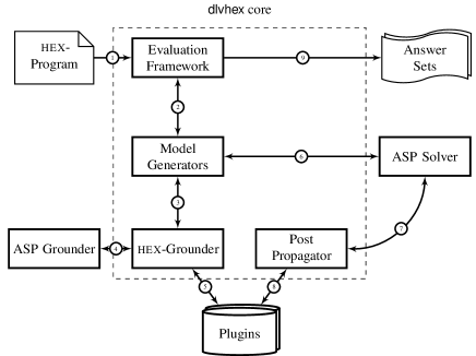
Figure 9: Architecture of dlvhex

6.2 Heuristics

As for creating evaluation graphs, several heuristics have been implemented. A heuristics starts with the rule dependency graph as by Definition 10 and then acyclically combines nodes into units.

Some heuristics are described in the following.

H0  is a ‘trivial’ heuristics that makes units as small as possible. This is useful for debugging, however it generates the largest possible number of evaluation units and therefore incurs a large overhead. As a consequence H0 performs clearly worse than other heuristics and we do not report its performance in experimental results.

H1  is the evaluation heuristics of the dlvhex prototype version 1. H1 makes units as large as possible and has several drawbacks as discussed above.

H2  is a simple evaluation heuristics which has the goal of finding a compromise between the H0 and H1. It places rules into units as follows:

1. it puts rules $r_{1},r_{2}$ into the same unit whenever $r_{1}\rightarrow_{m,n}s$ and $r_{2}\rightarrow_{m,n}s$ for some rule $s$ and there is no rule $t$ such that exactly one of $r_{1},r_{2}$ depends on $t$;

2. it puts rules $r_{1},r_{2}$ into the same unit whenever $s\rightarrow_{m,n}r_{1}$ and $s\rightarrow_{m,n}r_{2}$ for some rule $s$ and there is no rule $t$ such that $t$ depends on exactly one of $r_{1},r_{2}$; but

3. it never puts rules $r,s$ into the same unit if $r$ contains external atoms and $r\rightarrow_{m,n}s$.

Intuitively, H2 builds an evaluation graph that puts all rules with external atoms and their successors into one unit, while separating rules creating input for distinct external atoms. This avoids redundant computation and joining unrelated interpretations.

H3  is a heuristics for finding a compromise between (1) minimizing the number of units, and (2) splitting the program whenever a de-relevant nonmonotonic external atom would receive input from the same unit. We mention this heuristics only as an example, but disregard it in the experiments since it was developed in connection with novel ‘liberal’ safety criteria [Eiter et al. (2013)] that are beyond the scope of this paper. H3 greedily gives preference to (1) and is motivated by the following considerations. The grounding algorithm by ?) evaluates the external sources under all interpretations such that the set of observed constants is maximized. While monotonic and antimonotonic input atoms are not problematic (the algorithm can simply set all to true resp. false), nonmonotonic parameters require an exponential number of evaluations in general. Thus, although program decomposition is not strictly necessary for evaluating liberally safe hex-programs, it is still useful in such cases as it restricts grounding to those interpretations that are actually relevant in some answer set. However, on the other hand it can be disadvantageous for propositional solving algorithms such as those in [Eiter et al. (2012)].

Program decomposition can be seen as a hybrid between traditional and lazy grounding (cf. e.g. ?)), as program parts are instantiated that are larger than single rules but smaller than the whole program.

6.3 Experimental Results

In this section, we evaluate the model-building framework empirically. To this end, we compare the following configurations. In the H1 column, we use the previous state-of-the-art evaluation method [Schindlauer (2006)] before the framework in Section 5 was developed. This previous method also makes use of program decomposition. However, in contrast to our new framework, the decomposition is based on atom dependencies rather than rule dependencies, and the decomposition strategy is hard-coded and not customizable. This evaluation method corresponds to heuristics H1 in our new framework.

In the w/o framework column, we present the results without application of the framework using the hex-program evaluation algorithm by ?) which allows to first instantiate and then solve the instantiated hex-program. Note that before this algorithm was developed, such a ‘two-phase’ evaluation was not possible since program decomposition was necessary for grounding purposes. With the algorithm in [Eiter et al. (2014a)], decomposition is not necessary anymore, but can still be useful as the results in the H2 column shows, which correspond to the results when applying the heuristics H2 described above.

The configuration of the grounding algorithm and the solving algorithm (e.g., conflict-driven learning strategies) also influence the results. Moreover, in addition to the default heuristics of framework, other heuristics have been developed as well and the best selection of the heuristics often depends on the configuration of the grounding and the solving algorithm. Since they were used as black boxes in Algorithm 1, an exhaustive experimental analysis of the system is beyond the scope of this paper and would require an in-depth description of these algorithms. Thus, we confine the discussion to the default settings, which suffices to show that the new framework can speed up the evaluation significantly. The only configuration difference between the result columns H1 and H2 is the evaluation heuristics, all other parameters are equal. Evaluating the w/o framework column requires the grounding algorithm from [Eiter et al. (2014a)] instead of evaluation via decomposition, therefore w/o framework does not use any heuristics. The solver backend (clasp) configuration is the same in H1, H2, and w/o framework. We use the streaming algorithm (see C) in all experiments. For an in depth discussion, we refer to [Eiter et al. (2014b)] (?; ?) and ?), where the efficiency was evaluated using a variety of applications including planning tasks (e.g., robots searching an unknown area for an object, tour planning), computing extensions of abstract argumentation frameworks, inconsistency analysis in multi-context systems, and reasoning over description logic knowledge bases.

We discuss here two benchmark problems, which we evaluated on a Linux server with two 12-core AMD 6176 SE CPUs with 128GB RAM running dlvhex version 2.4.0. and an HTCondor load distribution system that ensures robust runtimes. The HTCondor system ensures that multiple runs of the same instance have negligible deviations in the order of fractions of a second, thus we can restrict the experiments to one run. The grounder and solver backends for all benchmarks are gringo 4.4.0 and clasp 3.1.1. For each instance, we limited the CPU usage to two cores and 8GB RAM. The timeout for each instance was 600 seconds. Each line shows the average runtimes over all instances of a certain size, where each timeout counts as 600 seconds. While instances usually become harder with larger size, there might be some exceptions due to the randomly generated instances; however, the overall trend shows that runtimes increase with the instance size. Numbers in parentheses are the numbers of instances of respective size in the leftmost column and the numbers of timeout instances elsewhere. The generators, instances and external sources are available at http://www.kr.tuwien.ac.at/research/projects/hexhex/hexframework.

6.3.1 Multi-Context Systems (MCS)

The MCS benchmarks originate in the application scenario of enumerating output-projected equilibria (i.e., global models) of a given multi-context system (MCS) (cf. Section 2.3.2). Each instance comprises 7–9 contexts (propositional knowledge bases) whose local semantics is modeled by external atoms; roughly speaking, they single out assignments to the atoms of a context occurring in bridge rules such that local models exist. For each context, 5–10 such atoms are guessed and bridge rules, which are modeled by ordinary rules, are randomly constructed on top. The MCS instances were generated using the DMCS [Bairakdar et al. (2010)] instance generator, with 10 randomized instances for different link structure between contexts (diamond (d), house (h), ring (r), zig-zag (z)) and system size; they have between 4 and about 20,000 answer sets, with an average of 400. We refer to [Bairakdar et al. (2010)] and [Schüller (2012)] for more details on the benchmarks and the hex-programs.

Topology and	First Answer Set			All Answer Sets
Instance Size	H1	w/o framework	H2	H1	w/o framework	H2
d-7-7-3-3 (10)	1.23 (0)	0.29 (0)	0.38 (0)	4.93   (0)	0.76 (0)	0.79 (0)
d-7-7-4-4 (10)	18.43 (0)	1.09 (0)	0.76 (0)	50.78   (0)	3.39 (0)	1.80 (0)
d-7-7-5-5 (10)	94.18 (1)	3.60 (0)	1.52 (0)	289.35   (4)	20.21 (0)	4.97 (0)
h-9-9-3-3 (10)	83.17 (1)	3.77 (0)	0.70 (0)	300.96   (4)	28.67 (0)	2.11 (0)
h-9-9-4-4 (10)	389.74 (6)	30.56 (0)	2.14 (0)	555.94   (9)	335.11 (5)	12.56 (0)
r-7-7-4-4 (10)	39.27 (0)	2.82 (0)	0.33 (0)	366.17   (5)	57.26 (0)	2.06 (0)
r-7-7-5-5 (10)	389.88 (6)	105.80 (1)	0.93 (0)	600.00 (10)	377.37 (5)	4.39 (0)
r-7-8-5-5 (10)	226.04 (3)	25.11 (0)	0.57 (0)	541.80   (9)	317.64 (5)	3.99 (0)
r-7-9-5-5 (10)	355.37 (5)	145.99 (2)	0.87 (0)	600.00 (10)	458.14 (7)	5.42 (0)
r-8-7-5-5 (10)	502.64 (8)	329.47 (5)	1.21 (0)	555.26   (9)	443.15 (7)	5.84 (0)
r-8-8-5-5 (10)	390.81 (6)	201.08 (3)	1.00 (0)	600.00 (10)	495.41 (8)	5.38 (0)
z-7-7-3-3 (10)	2.34 (0)	0.32 (0)	0.44 (0)	9.17   (0)	1.13 (0)	1.00 (0)
z-7-7-4-4 (10)	33.32 (0)	1.58 (0)	1.07 (0)	182.44   (2)	9.00 (0)	2.67 (0)
z-7-7-5-5 (10)	164.33 (2)	12.69 (0)	3.52 (0)	502.49   (8)	89.01 (1)	6.90 (0)

Table 1: MCS experiments: variable topology (d, h, r, z) and instance size.

Table 1 shows the experimental results: computation with the old method H1 often exceeds the time limit, while the new method H2 manages to enumerate all solutions of all instances. Monolithic evaluation without decomposition shows a performance between the old and new method. These results show that our new evaluation method is essential for using HEX to computationally realize the MCS application.

6.3.2 Reviewer Selection (RS)

Our second benchmark is Reviewer Selection (RS): we represent $c$ conference tracks, $r$ reviewers and $p$ papers. Papers and reviewers are assigned to conference tracks, and there are conflicts between reviewers and papers, some of which are given by external atoms. We consider two scenarios: RSTrack and RSPaper. They are designed to measure the effect of external atoms on the elimination of a large number of answer set candidates; in contrast to the MCS experiments we can control this aspect in the RS experiments.

In RSTrack we vary the number $c$ of conference tracks, where each track has 20 papers and 20 reviewers. Each paper must get two reviews, and no reviewer must get more than two papers. Conflicts are dense such that only one valid assignment exists per track, hence each instance has exactly one answer set, and in each track two conflicts are external. For each number $c$ there is only one instance because RSTrack instances are not randomized. The results of RSTrack are shown in Table 2: runtimes of the old evaluation heuristics (H1) grow fastest with size, without using decomposition grows slightly slower but also reaches timeout at size 9. Only the new decomposition (H2 heuristics) can deal with size 20 without timeout. Finding the first answer set and enumerating all answer sets show very similar times, as RSTrack instances have a single answer set and finding it seems hard.

Instance Size	First Answer Set			All Answer Sets
	H1	w/o framework	H2	H1	w/o framework	H2
1 (1)	2.84 (0)	3.14 (0)	2.78 (0)	2.73 (0)	3.14 (0)	2.79 (0)
2 (1)	6.13 (0)	7.18 (0)	4.90 (0)	6.05 (0)	7.17 (0)	4.88 (0)
3 (1)	10.18 (0)	12.30 (0)	8.32 (0)	10.25 (0)	12.35 (0)	8.37 (0)
4 (1)	15.92 (0)	18.66 (0)	12.12 (0)	15.86 (0)	18.85 (0)	12.16 (0)
5 (1)	26.06 (0)	28.47 (0)	17.17 (0)	26.23 (0)	28.35 (0)	17.06 (0)
6 (1)	47.06 (0)	45.71 (0)	23.39 (0)	46.84 (0)	45.62 (0)	23.26 (0)
7 (1)	92.76 (0)	79.41 (0)	31.19 (0)	96.56 (0)	79.82 (0)	31.04 (0)
8 (1)	198.59 (0)	155.10 (0)	37.85 (0)	199.74 (0)	155.26 (0)	38.06 (0)
9 (1)	600.00 (1)	600.00 (1)	46.61 (0)	600.00 (1)	600.00 (1)	46.75 (0)
10 (1)	600.00 (1)	600.00 (1)	57.48 (0)	600.00 (1)	600.00 (1)	57.40 (0)
11 (1)	600.00 (1)	600.00 (1)	68.98 (0)	600.00 (1)	600.00 (1)	69.45 (0)
12 (1)	600.00 (1)	600.00 (1)	84.41 (0)	600.00 (1)	600.00 (1)	84.11 (0)
13 (1)	600.00 (1)	600.00 (1)	99.55 (0)	600.00 (1)	600.00 (1)	99.52 (0)
14 (1)	600.00 (1)	600.00 (1)	117.39 (0)	600.00 (1)	600.00 (1)	117.15 (0)
15 (1)	600.00 (1)	600.00 (1)	138.45 (0)	600.00 (1)	600.00 (1)	137.51 (0)
16 (1)	600.00 (1)	600.00 (1)	163.12 (0)	600.00 (1)	600.00 (1)	158.43 (0)
17 (1)	600.00 (1)	600.00 (1)	184.99 (0)	600.00 (1)	600.00 (1)	181.94 (0)
18 (1)	600.00 (1)	600.00 (1)	208.83 (0)	600.00 (1)	600.00 (1)	210.82 (0)
19 (1)	600.00 (1)	600.00 (1)	236.98 (0)	600.00 (1)	600.00 (1)	237.45 (0)
20 (1)	600.00 (1)	600.00 (1)	267.54 (0)	600.00 (1)	600.00 (1)	268.60 (0)
21 (1)	600.00 (1)	600.00 (1)	600.00 (1)	600.00 (1)	600.00 (1)	600.00 (1)

Table 2: RSTrack experiments: variable number of conference tracks, single answer set.

In RSPaper we fix the number of tracks to $c\,{=}\,5$; we vary the number $p$ of papers in each track and set the number of reviewers to $r\,{=}\,p$. Each paper must get three reviews and each reviewer must not get more than three papers assigned. Conflicts are randomized and less dense than in RSTrack: the number of answer sets is greater than one and does not grow with the instance size. Over all tracks and papers, $2p$ randomly chosen conflicts are external, and we generate 10 random instances per size and report results averaged per instance size in Table 3. As clearly seen, our new method is always faster than the other methods, and evaluation without a decomposition framework performs slightly better than the old method. Different from RSTrack, we can see a clear difference between finding the first answer set and enumerating all answer sets as RSPaper instances have more than one answer set.

To confirm that the new method is geared towards handling many external atoms, we conducted also experiments with instances that had few external atoms for eliminating answer set candidates but many local constraints. For such highly constrained instances, the new decomposition framework is not beneficial as it incurs an overhead compared to the monolithic evaluation that increases runtimes.

Instance Size	First Answer Set			All Answer Sets
	H1	w/o framework	H2	H1	w/o framework	H2
5 (10)	1.06   (0)	0.28   (0)	0.21 (0)	2.25   (0)	0.43   (0)	0.23   (0)
8 (10)	8.76   (0)	2.73   (0)	0.38 (0)	14.73   (0)	4.54   (0)	0.44   (0)
11 (10)	108.70   (1)	83.26   (1)	0.98 (0)	171.01   (2)	104.84   (1)	1.28   (0)
14 (10)	180.99   (2)	125.83   (1)	2.08 (0)	299.22   (4)	245.62   (3)	2.67   (0)
17 (10)	418.92   (6)	364.95   (5)	5.15 (0)	549.01   (9)	513.21   (8)	8.14   (0)
20 (10)	485.35   (8)	453.39   (7)	7.32 (0)	507.66   (8)	501.74   (8)	14.45   (0)
23 (10)	542.03   (9)	508.75   (8)	13.91 (0)	600.00 (10)	600.00 (10)	23.16   (0)
26 (10)	600.00 (10)	600.00 (10)	33.20 (0)	600.00 (10)	600.00 (10)	154.51   (2)
29 (10)	600.00 (10)	600.00 (10)	60.78 (0)	600.00 (10)	600.00 (10)	108.03   (0)
32 (10)	600.00 (10)	600.00 (10)	129.95 (0)	600.00 (10)	600.00 (10)	315.56   (4)
35 (10)	600.00 (10)	600.00 (10)	136.84 (0)	600.00 (10)	600.00 (10)	302.90   (3)
38 (10)	600.00 (10)	600.00 (10)	308.92 (3)	600.00 (10)	600.00 (10)	441.06   (6)
41 (10)	600.00 (10)	600.00 (10)	421.69 (6)	600.00 (10)	600.00 (10)	529.80   (8)
44 (10)	600.00 (10)	600.00 (10)	470.61 (7)	600.00 (10)	600.00 (10)	553.19   (9)
47 (10)	600.00 (10)	600.00 (10)	485.60 (7)	600.00 (10)	600.00 (10)	529.00   (8)
50 (10)	600.00 (10)	600.00 (10)	485.07 (7)	600.00 (10)	600.00 (10)	526.66   (8)

Table 3: RSPaper experiments: variable number of papers/reviewers, multiple answer sets, randomized.

6.3.3 Summary

The results demonstrate a clear improvement using the new framework; they can often be further improved by fine-tuning the grounding and solving algorithm, and by customizing the default heuristics of the framework, as discussed by [Eiter et al. (2014b)] (?; ?), and ?). However, already the default settings yield results that are significantly better than using the previous evaluation method or using no framework at all; note that the latter requires an advanced grounding algorithm as by ?), which was not available at the time the initial evaluation approach as by ?) was developed.

In conclusion, the evaluation framework in Section 5 pushes hex-programs towards scalability for realistic instance sizes, which previous evaluation techniques missed.

7 Related Work and Discussion

We now discuss our results in the context of related work, and will address possible optimizations.

7.1 Related Work

We first discuss related approaches for integrating external reasoning into ASP formalisms, then we discuss work related to the notion of rule dependencies that we introduced in Section 4.1, we discuss related notions of modularity and program decomposition. Finally we relate our splitting theorems to other splitting theorems in the literature.

7.1.1 External Sources

The dlv-ex system [Calimeri et al. (2007)] was a pioneering work on value invention through external atoms in ASP. It supported VI-restricted programs, which amount to hex-programs under extensional semantics without higher-order atoms and a strong safety condition that is subsumed by lde-safety. Answer set computation followed the traditional approach on top of dlv, but used a special progressive grounding method (thus an experimental comparison to solving, i.e., model building as in the focus of this paper, is inappropriate).

With respect to constraint theories and ASP, several works exist. The ACsolver system [Mellarkod et al. (2008)], the ezcsp system [Balduccini (2009)], and the clingcon system [Ostrowski and Schaub (2012)] divide the program into ASP-literals and constraint-literals, which can be seen as a special case of hex-programs that focuses on a particular external source. As for evaluation, an important difference to general external sources is that constraint atoms do not use value invention. The modularity techniques from above are less relevant for this setting as grounding the overall program in one shot is possible. However, this also fits into our framework as disabling decomposition in fact corresponds to a dedicated (trivial) heuristics which keeps the whole program as a single unit. For a detailed comparison between ACsolver, ezcsp, and clingcon  see [Lierler (2014)].

?) also experimentally compared ezcsp and clingcon while varying the degree of integration between the constraint solver and the ASP solver backend. Their ‘black-box integration’ corresponds with dlvhex’s integration of the dlv backend: external atom semantics are verified by plugins callbacks only when a full answer set candidates has been found in the backend; moreover their ‘clear-box integration’ corresponds with dlvhex’s integration of the clasp solver backend: plugin callbacks are part of the CDCL propagation and can operate on partial answer set candidates. Note that constraint answer set programs can be realized as a dlvhex-plugin (such an effort is currently ongoing).

We also remark that gringo and clasp use a concept called ‘external atoms’ for realizing various applications such as constraint ASP solving as in clingcon and incremental solving [Gebser et al. (2014)]. However, despite their name they are different from external atoms in hex-programs. In the former case, external atoms are excluded from grounding-time optimization such that these atoms are not eliminated even if their truth value is deterministically false during grounding. This allows to add rules that found truth of such atoms in later incremental grounding steps. In case of hex the truth value is determined by external sources. Moreover gringo contains an interface for Lua and Python functions that can perform computations during grounding. hex external atoms are more expressive: they cannot always be evaluated during grounding because their semantics is defined with respect to the answer set.

7.1.2 Rule Dependencies

In the context of answer set programming, dependency graphs over rules have been used earlier, e.g., by ?) and ?). However, these works consider only ordinary ground programs, and furthermore the graphs are used for characterizing and computing the answer sets of a program from these graphs. In contrast, we consider nonground programs with and external atoms, and we use the graph to split the program into evaluation units with the goal of modularly computing answer sets.

7.1.3 Modularity

Our work is naturally related to work on program modularity under stable model semantics, as targeted by splitting sets [Lifschitz and Turner (1994)] and descendants, with the work by ?) and ?) a prominent representative that lifted them to modular programs with choice rules and disjunctive rules, by considering ‘symmetric splitting’. Other works, e.g., by ?) go further to define semantics of systems of program modules, departing from a mere semantics-preserving decomposition of a larger program into smaller parts, or consider multi-language systems that combine modules in possibly different formalisms on equal terms (cf. e.g. ?) and ?)).

Comparing the works by ?) and ?) as, from a semantic decomposition perspective, the closest in this group to ours, an important difference is that our approach works for non-ground programs and explicitly considers possible overlaps of modules. It is tailored to efficient evaluation of arbitrary programs, rather than to facilitate module-style logic programming with declarative specifications, or to provide compositional semantics for modules beyond uni-lateral evaluation, as done by ?) and ?); for them, introducing values outside the module domain (known as value invention) does not play a visible role. In this regard, it is in line with previous hex-program evaluation [Eiter et al. (2006)] and decomposition techniques to ground ordinary programs efficiently [Calimeri et al. (2008)].

7.1.4 Splitting Theorems

Our new splitting theorems compare to related splitting theorems as follows.

Theorem 1 is similar to Theorem 4.6.2 by ?); however, we do not use splitting sets on atoms, but splitting sets on rules. Furthermore, ?) has no analog to Theorem 2.

The seminal Splitting Set Theorem by ?) divides the interpretation of $P$ into disjoint sets $X$ and $Y$, where $X$ is an answer set of the ‘bottom’ $\mathit{gb}_{A}(P)\subseteq P$ and $Y$ is an answer set of a ‘residual’ program obtained from $P\setminus\mathit{gb}_{A}(P)$ and $X$. In the residual program, all references to atoms in $X$ are removed, in a way that it semantically behaves as if facts $X$ were added to $P\setminus\mathit{gb}_{A}(P)$, while the answer sets of the residual do not contain any atom in $X$. This works nicely for answer set programs, but it is problematic when applied to hex programs, because external atoms may depend on the bottom and on atoms in heads of the residual program; hence, they cannot be eliminated from rule bodies. The only way to eliminate bottom facts from the residual program would be to ‘split’ external atoms semantically into a part depending on the bottom and the program remainder, and by replacing external atoms in rules with external atoms that have been partially evaluated wrt. a bottom answer set. Technically, this requires to introduce new external atoms, and formulating a splitting theorem for hex programs with two disjoint interpretations $X$ and $Y$ is not straightforward. Furthermore, such external atom splitting and partial evaluation might not be possible in a concrete application scenario.

Different from the two splitting theorems recalled above, the Global Splitting Theorem by ?) does not split an interpretation of the program $P$ into disjoint interpretations $X$ and $Y$, and thus should be compared to our Theorem 2. However, the Global Splitting Theorem does not allow constraint sharing, and it involves a residual program which specifies how external atoms are evaluated via ‘replacement atoms’, which lead to extra facts $D$ in the residual program that must be removed from its answer sets. Both the specification of replacement atoms and the extra facts make the Global Splitting Theorem cumbersome to work with when proving correctness of hex encodings. Moreover, the replacement atoms are geared towards a certain implementation technique which however is not mandatory and can be avoided.

Lemma 5.1 by ?) is structurally similar to our Theorem 2: answer sets of the bottom program are evaluated together with the program depending on the bottom (here called the residual), hence answer sets of the residual are answer sets of the original program. However, the result was based on atom dependencies and did neither consider negation nor external atoms.

In sumary our new Generalized Splitting Theorem has the following advantages.

• By moving from atom to rule splitting sets, no separate definition of the bottom is needed, which just becomes the (rule) splitting set.

• As regards hex-programs, splitting is simple (and not troubled) if all atoms that are true in an answer set of the bottom also appear in the residual program. Typically, this is not the case in results from the literature.

• Finally, also the residual program itself is simpler (and easier to construct), by just dropping rules and adding facts. No rule rewriting needs to be done, and no extra facts need to be introduced in the residual program nor in the bottom.

The only (negligible) disadvantage of the new theorems is that the answer sets of the bottom and the residual program may no longer be disjoint; however, each residual answer set includes some (unique) bottom answer set.

7.2 Possible Optimizations

Evaluation graphs naturally encode parallel evaluation plans. We have not yet investigated the potential benefits of this feature in practice, but this property allows us to do parallel solving based on solver software that does not have parallel computing capabilities itself (‘parallelize from outside’). This applies both to programs with external atoms, as well as to ordinary ASP programs (i.w., without external atoms). Improving reasoning performance by decomposition has been investigated by ?), however, only wrt. monotonic logics.

Improving hex evaluation efficiency by using knowledge about domain restrictions of external atoms has been discussed by ?). These rewriting methods yield partially grounded sets of rules which can easily be distributed into distinct evaluation units by an optimizer. This directly provides efficiency gains as described in the above work.

As a last remark on possible optimizations, we observe that the data flow between evaluation units can be optimized using proper notions of model projection, such as in [Gebser et al. (2009a)]. Model projections would tailor input data of evaluation units to necessary parts of intermediate answer sets; however, given that different units might need different parts of the same intermediate input answer set, a space-saving efficient projection technique is not straightforward.

8 Conclusion

hex-programs extend answer set programs with access to external sources through an API-style interface, which has been fruitfully deployed to various applications. Providing efficient evaluation methods for such programs is a challenging but important endeavor, in order to enhance the practicality of the approach and to make it eligible for a broader range of applications. In this direction, we have presented in this article a novel evaluation method for hex-programs based on modular decomposition. We have presented new results for the latter using special splitting sets, which are more general than previous results and use rule sets as a basis for splitting rather than sets of atoms as in previous approaches. Furthermore, we have presented an evaluation framework which employs besides a traditional evaluation graph that consists of program components and reflects syntactic dependencies among them, also a model graph whose nodes collect answer sets that are combined and passed on between components. Using decomposition techniques, evaluation units can be dynamically formed and evaluated in the framework using different heuristics, Moreover, the answer sets of the overall program can be produced in a streaming fashion. The new approach leads in combination with other techniques to significant improvements for a variety of applications, as demonstrated by [Eiter et al. (2014a)] (?; ?) and ?). Notably, while our results target hex-programs, the underlying concepts and techniques are not limited to them (e.g., to separate the evaluation and the model graph) and may be fruitfully transferred to other rule-based formalisms.

8.1 Outlook

The work we presented can be continued in different directions. As for the prototype reasoner, a rather straightforward extension is to support brave and cautious reasoning on top of hex programs, while incorporating constructs like aggregates or preference constraints requires more care and efforts. Regarding program evaluation, our general evaluation framework provides a basis for further optimizations and evaluation strategies. Indeed, the generic notions of evaluation unit, evaluation graph and model graph allow to specialize and improve our framework in different respects. First, evaluation units (which may contain duplicated constraints), can be chosen according to a proper estimate of the number of answer sets (the fewer, the better); second, evaluation plans can be chosen by ad-hoc optimization modules, which may give preference to (a combination of) time, space, or parallelization conditions. Third, the framework is amenable to a form of coarse-grained distributed computation at the level of evaluation units (in the style of ?)).

While modular evaluation is advantageous in many applications, it can also be counterproductive, as currently the propagation of knowledge learned by conflict-driven techniques into different evaluation units is not possible. In such cases, evaluating the program as a single evaluation unit is often also infeasible due to the properties of the grounding algorithm, as observed by ?). Thus, another starting point for future work is a tighter integration of the solver instances used to evaluate different units, e.g., by exchanging learned knowledge. In this context, also the interplay of the grounder and the solver is an important topic.

Appendix A Proofs

Proof A.7 (Proof of Theorem 1 (Splitting Theorem)).

Given a set of ground atoms $M$ and a set of rules $R$, we denote by $M|_{R}=M\cap{\mathit{gh}(R)}$ the projection of $M$ to ground heads of rules in $R$.

($\Rightarrow$) Let $M\in\mathcal{A\!S}(P)$. We show that (1) ${M|_{R}}\in\mathcal{A\!S}(R)$ and that (2) $M\in\mathcal{A\!S}(P\setminus R\cup\mathit{facts}({M|_{R}}))$.

As for (1), we first show that ${M|_{R}}$ satisfies the reduct $fR^{M|_{R}}$, and then that ${M|_{R}}$ is indeed a minimal model of $fR^{M|_{R}}$. $M$ satisfies $fP^{M}$ and $R\subseteq P$. Observe that, by definition of FLP reduct, $fR^{M}\subseteq fP^{M}$. By definition of rule splitting set, satisfiability of rules in $R$ does not depend on heads of rules in $P\setminus R$ (due to the restriction of external atoms to extensional semantics, this is in particular true for external atoms in $R$). Therefore $fR^{M|_{R}}=fR^{M}$, $M$ satisfies $fR^{M|_{R}}$, and ${M|_{R}}$ satisfies $fR^{M|_{R}}$. For showing ${M|_{R}}\in\mathcal{A\!S}(R)$, it remains to show that ${M|_{R}}$ is a minimal model of $fR^{M|_{R}}$.

Assume towards a contradiction that some $S\subset{M|_{R}}$ is a model of $fR^{M|_{R}}$. Then there is a nonempty set $A={M|_{R}}\setminus S$ of atoms with $A\subseteq{\mathit{gh}(R)}$. Let $M^{\star}=M\setminus A$. We next show that $M^{\star}$ is a model of $fP^{M}$, which implies that $M\notin\mathcal{A\!S}(P)$. Assume on the contrary that $M^{\star}$ is not a model of $fP^{M}$. Hence there exists some rule $r\in fP^{M}$ such that $H(r)\cap M^{\star}=\emptyset$, $B^{+}(r)\subseteq M^{\star}$, $B^{-}(r)\cap M^{\star}=\emptyset$ and external atoms in $B^{+}(r)$ (resp., $B^{-}(r)$) evaluate to true (resp., false) wrt. $M^{\star}$. $S$ agrees with $M^{\star}$ on atoms from ${\mathit{gh}(R)}$, and $S$ satisfies $fR^{M|_{R}}$. The truth values of external atoms in bodies of rules in $R$ depends only on atoms from ${\mathit{gh}(R)}$, therefore external atoms in $R$ evaluate to the same truth value wrt. $S$ and $M^{\star}$. Therefore $r\notin fR^{M|_{R}}$ and $r\in f(P\setminus R)^{M}$. Since $r\in P\setminus R$, $H(r)\subseteq{\mathit{gh}(P\setminus R)}$, and because $M$ and $M^{\star}$ agree on atoms from ${\mathit{gh}(P\setminus R)}$, $H(r)\cap M^{\star}=\emptyset$ from above implies that $H(r)\cap M=\emptyset$. Because $r\in fP^{M}$, its body is satisfied in $M$, and since its head has no intersection with $M$, we get that $fP^{M}$ is not satisfied by $M$, which is a contradiction. Therefore $M^{\star}$ is a model of $fP^{M}$. As $M^{\star}\,{\subset}\,M$, this contradicts our assumption that $M\in\mathcal{A\!S}(P)$. Therefore $S={M|_{R}}=X$ is a minimal model of $fR^{M}$.

We next show that $M$ satisfies the reduct $f(P\setminus R\cup\mathit{facts}({M|_{R}}))^{M}$, and then that it is indeed a minimal model of the reduct. By the definition of reduct, $f(P\setminus R\cup\mathit{facts}({M|_{R}}))^{M}=f(P\setminus R)^{M}\cup\mathit{facts}({M|_{R}})$. $M$ satisfies $\mathit{facts}({M|_{R}})$ because ${M|_{R}}\subseteq M$. Furthermore $f(P\setminus R)^{M}\subseteq fP^{M}$, hence $M$ satisfies $f(P\setminus R)^{M}$. Therefore $M$ satisfies $f(P\setminus R\cup\mathit{facts}({M|_{R}}))^{M}$.

To show that $M$ is a minimal model of $f(P\setminus R\cup\mathit{facts}({M|_{R}}))^{M}$, assume towards a contradiction that some $S\,{\subset}\,M$ is a model of $f(P\setminus R\cup\mathit{facts}({M|_{R}}))^{M}$. Since $\mathit{facts}({M|_{R}})$ is part of the reduct, ${M|_{R}}\subseteq S$, therefore $S|_{\mathit{gh}(R)}={M|_{R}}$. By definition of rule splitting set, satisfiability of rules in $R$ does not depend on heads of rules in $P\setminus R$, hence $S$ satisfies $fR^{M}$. Because $S$ satisfies $f(P\setminus R\cup\mathit{facts}({M|_{R}}))^{M}=f(P\setminus R)^{M}\cup\mathit{facts}({M|_{R}})$, it also satisfies $f(P\setminus R)^{M}$. Since $S$ satisfies both $fR^{M}$, $S$ satisfies $fP^{M}=f(P\setminus R)^{M}\cup fR^{M}$. This is a contradiction to $M\in\mathcal{A\!S}(P)$. Therefore $S=M$ is a minimal model of $f(P\setminus R\cup\mathit{facts}({M|_{R}}))^{M}$.

($\Leftarrow$) Let $M\in\mathcal{A\!S}(P\setminus R\cup\mathit{facts}(X))$ and let $X\in\mathcal{A\!S}(R)$. We first show that $M$ satisfies $fP^{M}$, and then that it is a minimal model of $fP^{M}$.

As facts $X$ are part of the program $P\setminus R\cup\mathit{facts}(X)$, and by definition of rule splitting set, $P\setminus R$ contains no rule heads unifying with ${\mathit{gh}(R)}$, hence we have $X={M|_{R}}$. Furthermore $f(P\setminus R\cup\mathit{facts}(X))^{M}\setminus\mathit{facts}(X)\cup fR^{M}=fP^{M}$, and as $M$ satisfies the left side, it satisfies the right side. To show that $M$ is a minimal model of $fP^{M}$, assume $S\,{\subset}\,M$ is a smaller model of $fP^{M}$. By definition of reduct, $S$ also satisfies $f(P\setminus R)^{M}$ and $fR^{M}$. Since $R$ is a splitting set, satisfiability of rules in $R$ does not depend on heads of rules in $P\setminus R$, therefore $fR^{M}=fR^{M|_{R}}=fR^{X}$ and $S|_{{\mathit{gh}(R)}}$ satisfies $fR^{X}$. Since $S\subset M$, we have $S|_{{\mathit{gh}(R)}}\subseteq X$. Because $X$ is a minimal model of $fR^{X}$, $S|_{{\mathit{gh}(R)}}\subset X$ is impossible and $S|_{{\mathit{gh}(R)}}=X$. Therefore $S|_{{\mathit{gh}(P\setminus R)}}\subset M|_{{\mathit{gh}(P\setminus R)}}$. Because $S$ satisfies $f(P\setminus R)^{M}$ and $S|_{{\mathit{gh}(R)}}=X$, $S$ also satisfies $f(P\setminus R\cup\mathit{facts}(X))^{M}$. Since $S\subset M$, this contradicts the fact that $M$ is a minimal model of $P\setminus R\cup\mathit{facts}(X)$. Therefore $S=M$ is a minimal model of $fP^{M}$.

Proof A.8 (Proof of Theorem 2 (Generalized Splitting Theorem)).

By definition of generalized bottom, the set $C=B\setminus R$ contains only constraints, therefore ${\mathit{gh}(B)}={\mathit{gh}(R)}$ and ${M|_{{\mathit{gh}(B)}}}={M|_{{\mathit{gh}(R)}}}$. As $R\subseteq B$ and $B\setminus R$ contains only constraints, $\mathcal{A\!S}(B)\subseteq\mathcal{A\!S}(R)$. The only difference between Theorem 1 and Theorem 2 is, that for obtaining $X$, the latter takes additional constraints into account.

($\Rightarrow$) It is sufficient to show that ${M|_{{\mathit{gh}(B)}}}$ does not satisfy the body of any constraint in $C\subseteq P$ if $M$ does not satisfy the body of any constraint in $P$. Since $B$ is a generalized bottom, no negative dependencies of constraints $C$ to rules in $P\setminus B$ exist; therefore if the body of a constraint $c\in C$ is not satisfied by $M$, the body of $c$ is not satisfied by ${M|_{{\mathit{gh}(B)}}}$. As $M$ satisfies $P$, it does not satisfy any constraint body in $P$, hence the projection ${M|_{{\mathit{gh}(B)}}}$ does not satisfy any constraint body in $B\setminus R$.

($\Leftarrow$) It is sufficient to show that an answer set of $R$ that satisfies a constraint body in $C$ also satisfies that constraint body in $P$, which raises a contradiction. As constraints in $C$ have no negative dependencies to rules in $P\setminus B$, a constraint with a satisfied body in ${M|_{{\mathit{gh}(R)}}}$ also has a satisfied body in $M$, therefore the result follows.

Proof A.9 (Proof of Proposition 1).

Assume towards a contradiction that there exist a non-constraint $r\in P$, a rule $s\in P$ with $r\rightarrow_{m,n}s$, and $u^{\prime}\in U|_{r}$, $v^{\prime}\in U|_{s}$ such that $(u^{\prime},v^{\prime})\notin E$. Due to Definition 9, $r\rightarrow_{m,n}s$ implies that $s$ has $H(s)\neq\emptyset$ and therefore that $s$ is a non-constraint. Definition 14 (b) then implies that $U|_{r}=\{u^{\prime}\}$ and $U|_{s}=\{v^{\prime}\}$ (non-constraints are present in exactly one unit).

Case (i): for $r\rightarrow_{n}s$, Definition 14 (c) specifies that for all $u\in U|_{r}$ and $v\in U|_{s}$ there exists an edge $(u,v)\in E$, therefore also $(u^{\prime},v^{\prime})\in E$, which is a contradiction.

Case (ii): for $r\rightarrow_{m}s$, Definition 14 (d) specifies that some $u\in U|_{r}$ exists such that for every $v\in U|_{s}$ there exists an edge $(u,v)\in E$; since $U|_{r}=\{u^{\prime}\}$ and $U|_{s}=\{v^{\prime}\}$, it must hold that $(u^{\prime},v^{\prime})\in E$, which is a contradiction.

Proof A.10 (Proof of Proposition 2).

Given two distinct units $u_{1},u_{2}\in U$, assume towards a contradiction that some $\gamma\in{\mathit{gh}(u_{1})}\cap{\mathit{gh}(u_{2})}$ exists. Then there exists some $r\in u_{1}$ with $\alpha\in H(r)$ and $\alpha\sim\gamma$, and there exists some $s\in u_{2}$ with $\beta\in H(s)$ and $\beta\sim\gamma$. As $\alpha\sim\gamma$ and $\beta\sim\gamma$ and $\gamma$ is ground, we obtain $\alpha\sim\beta$; hence, by Definition 9 (iii) we have $r\rightarrow_{m}s$ and $s\rightarrow_{m}r$. As $r$ and $s$ have nonempty heads, they are non-constraints. Thus by Proposition 1, there exist edges $(u_{1},u_{2}),(u_{2},u_{1})\in E$. As an evaluation graph is acyclic, it follows $u_{1}=u_{2}$; this is a contradiction.

Proof A.11 (Proof of Proposition 3).

For an lde-safe program $P$, the graph ${\mathcal{E}}=(\{P\},\emptyset)$ is a valid evaluation graph.

Proof A.12 (Proof of Theorem 3).

For any set of rules, let $\mathit{constr}(S)=\{r\in S\mid{H}(r)=\emptyset\}$ denote the set of constraints in $S$. We say that the dependencies of $r\in Q$ are covered at unit $u\in U$, if for every rule $s\in Q$ such that $r\rightarrow_{m,n}s$ and $s\notin u$, it holds that $(u,u^{\prime})\in E$ for all $u^{\prime}\in U|_{s}$, i.e., $u$ has an edge to all units containing $s$.

To prove that $B=u^{<}$ is a generalized bottom of $P=u^{\leq}$ wrt. the rule splitting set $R=u^{<}\setminus\mathit{constr}(u^{<})$ as by Definition 12, we prove that (a) $R\subseteq B\subseteq P$, (b) $B\setminus R$contains only constraints, (c) no constraint in $B\setminus R$ has nonmonotonic dependencies to rules in $P\setminus B$, and (d) $R$is a rule splitting set of $P$.

Statement (a) corresponds to $u^{<}\setminus\mathit{constr}(u^{<})\subseteq u^{<}\subseteq u^{\leq}$ and $u^{\leq}$ is defined as $u^{\leq}=u^{<}\cup u$, therefore the relations all hold. For (b), $B\setminus R=u^{<}\setminus(u^{<}\setminus\mathit{constr}(u^{<}))$, and as $A\setminus(A\setminus B)=A\cap B$, it is easy to see that $B\setminus R=u^{<}\cap\mathit{constr}(u^{<})$ and thus $B\setminus R$ only contains constraints. For (c), we show a stronger property, namely that no rule (constraint or non-constraint) in $B$ has nonmonotonic dependencies to rules in $P\setminus B$. $B=u^{<}$ is the union of evaluation units $V=\{v\in U\mid v<u\}$. By Definition 14 (c) all nonmonotonic dependencies $r\rightarrow_{n}s$ are covered at every unit $w$ such that $w\in U_{r}$. Hence if $r\in w$ and $w\in V$, then either $s\in w$ or $s\in w^{<}$ holds, and hence $s\in w^{\leq}\subseteq u^{<}$. As $P\setminus B=u^{\leq}\setminus u^{<}$, no nonmonotonic dependencies from $B=u^{<}$ to $P\setminus B$ exist and (c) holds. For (d) we know that $R=u^{<}\setminus\mathit{constr}(u^{<})$ contains no constraints, and by Proposition 1 all dependencies of non-constraints in $R$ are covered by ${\mathcal{E}}$. Therefore $r\in R$, $r\rightarrow_{m,n}s$, and $s\in P$ implies that $s\in R$. Consequently, (d) holds which proves the theorem.

Proof A.13 (Proof of Theorem 4).

Similar to the proof of Theorem 3, we show this in four steps; given $P=u^{<}$, $R=u^{\prime\leq}\setminus\mathit{constr}(u^{\prime\leq})$, and $B=u^{\prime\leq}=u^{\prime}\cup u^{\prime<}$, we show that (a) $R\subseteq B\subseteq P$, (b) $B\setminus R$contains only constraints, (c) no constraint in $B\setminus R$ has nonmonotonic dependencies to rules in $P\setminus B$, and (d) $R$is a rule splitting set of $P$. Let $\mathit{preds}_{{\mathcal{E}}}(u)=\{u_{1},\ldots,u_{k}\}$ and Let $V=\{v\in U\mid v<u^{\prime}\}$ be the set of units on which $u^{\prime}$ transitively depends. (Note that $V\subset\mathit{preds}_{{\mathcal{E}}}(u)$ and $u\notin V$.) As $u^{\prime<}$ contains all units $u^{\prime}$ transitively depends on, we have $B=u^{\prime}\cup\bigcup_{w\in V}w$.

For (a), $R\subseteq B$ holds trivially, and $B\subseteq P$ holds by definition of $u^{<}$ and $u^{\prime\leq}$ and because $u^{\prime}\in\mathit{preds}_{{\mathcal{E}}}(u)$. Statement (b) holds, because $B\setminus R$ removes $R$ from $B$, i.e., it removes everything that is not a constraint in $B$ from $B$, therefore only constraints remain. For (c) we show that no rule in $B$ has a nonmonotonic dependency to rules in $P\setminus B$. By Definition 14 (c), all nonmonotonic dependencies are covered at all units. Therefore a rule $r\in w$, $w\in\{u^{\prime}\}\cup V$ with $r\rightarrow_{n}s$, $s\in U$ implies that either $s\in w$, or that $s$ is contained in a predecessor unit of $w$ and therefore in $u^{\prime}$ or in $V$. Hence there are no nonmonotonic dependencies from rules in $B$ to any rules not in $B$, and hence also not to rules in $P\setminus B$ and (c) holds. For (d) we know that $R$ contains no constraints and by Proposition 1 all dependencies of non-constraints in $R$ are covered by ${\mathcal{E}}$. Therefore $r\in R$, $r\rightarrow_{m,n}s$, $s\in P$ implies that $s\in R$ and the theorem holds.

Proof A.14 (Proof of Proposition 4).

($\Rightarrow$) The added vertex $m^{\prime}$ is assigned to one unit and gets assigned a type. Furthermore, the graph stays acyclic as only outgoing edges from $m^{\prime}$ are added. I-connectedness is satisfied, as it is satisfied in ${\mathcal{I}}$ and we add no o-interpretation. O-connectedness is satisfied, as $m^{\prime}$ gets appropriate edges to o-interpretations at its predecessor units, and for other i-interpretations it is already satisfied in ${\mathcal{I}}$.

For FAI intersection, observe that if we add an edge $(m^{\prime},m_{i})$ to ${\mathcal{I}}$ and it holds that $m_{i}\,{\in}\,\mathit{o\text{-}ints}_{{\mathcal{I}}}(u_{i})$, then $m^{\prime}$ reaches in ${\mathcal{I}}$ only one o-interpretation at $u_{i}$, and due to O-connectedness that o-interpretation is connected to exactly one i-interpretation at $u_{i}$, which is part of the original graph ${\mathcal{I}}$ and therefore satisfies FAI intersection. Therefore it remains to show that the union of subgraphs of ${\mathcal{I}}$ reachable in ${\mathcal{I}}$ from $m_{1}$,…,$m_{k}$, contains one o-interpretation at each unit in the subgraph of ${\mathcal{E}}$ reachable from $u_{1}$,…,$u_{k}$. We make a case distinction.

Case (I): two o-interpretations $m_{i}\in\mathit{o\text{-}ints}_{{\mathcal{I}}}(u_{i})$, $m_{j}\in\mathit{o\text{-}ints}_{{\mathcal{I}}}(u_{j})$ in the join, with $1\leq i<j\leq k$, have no common unit that is reachable in ${\mathcal{E}}$ from $u_{i}$ and from $u_{j}$: then the condition is trivially satisfied, as the subgraphs of ${\mathcal{I}}$ reachable in ${\mathcal{I}}$ from $m_{i}$ and $m_{j}$, respectively, do not intersect at any unit.

Case (II): two o-interpretations $m_{i}\in\mathit{o\text{-}ints}_{{\mathcal{I}}}(u_{i})$, $m_{j}\in\mathit{o\text{-}ints}_{{\mathcal{I}}}(u_{j})$ in the join, with $1\leq i<j\leq k$, have at least one common unit that is reachable from $u_{i}$ and from $u_{j}$ in ${\mathcal{E}}$. Let $u^{f}$ be a unit reachable in ${\mathcal{E}}$ from both $u_{i}$ and $u_{j}$ on two paths that do not intersect before reaching $u^{f}$. From $u_{i}$ to $u^{f}$, and from $u_{j}$ to $u^{f}$, exactly one o-interpretation is reachable in ${\mathcal{I}}$ from $m_{i}$ and $m_{j}$, respectively, as these paths do not intersect. $u^{f}$ is a FAI of $u$, and as the join is defined, we reach in ${\mathcal{E}}$ exactly one o-interpretation at unit $u^{f}$ from $m_{i}$ and $m_{j}$. Due to O-connectedness, we also reach in ${\mathcal{I}}$ exactly one i-interpretation $m^{\prime\prime}$ at $u^{f}$ from $m_{i}$ and $m_{j}$. Now $m^{\prime\prime}$ is common to subgraphs of ${\mathcal{I}}$ that are reachable in ${\mathcal{I}}$ from $m_{i}$ and $m_{j}$, and $m^{\prime\prime}$ satisfies FAI intersection in ${\mathcal{I}}$.

Consequently, FAI intersection is satisfied in ${\mathcal{I}}^{\prime}$ for all pairs of predecessors of $m^{\prime}$ and therefore in all cases. As no vertex $m$ with $\{(m,m_{1}),\ldots,(m,m_{k})\}\subseteq F$ exists and and as ${\mathcal{I}}$ satisfies Uniqueness, also ${\mathcal{I}}^{\prime}$ satisfies Uniqueness.

($\Leftarrow$) Assume towards a contradiction that ${\mathcal{I}}^{\prime}$ is an i-graph but that the join is not defined. Then there exists some FAI $u^{\prime}\in\mathit{fai}(u)$ such that either no or more than one o-interpretation from $\mathit{o\text{-}ints}_{{\mathcal{I}}}(u)$ is reachable in ${\mathcal{I}}$ from some $m_{i}$, $1\leq i\leq k$. As ${\mathcal{I}}$ is an i-graph, due to I-connectedness and O-connectedness, if a unit $u^{\prime}$ is a FAI and therefore $u^{\prime}$ is reachable in ${\mathcal{E}}$ from $u_{i}$, then at least one i-interpretation and one o-interpretation at $u^{\prime}$ is reachable in ${\mathcal{I}}$ from $m_{i}$. If more than one o-interpretation is reachable in ${\mathcal{I}}$ from some $m_{i}$, $1\leq i\leq k$, this means that more than one o-interpretation at $u^{\prime}$ is reachable in ${\mathcal{I}}^{\prime}$ from the newly added i-interpretation $m$. However, this violates FAI intersection in ${\mathcal{I}}^{\prime}$, which is a contradiction. Hence the result follows.

Proof A.15 (Proof of Proposition 5).

($\Rightarrow$) Whenever the join is defined, ${\mathcal{A}}^{\prime}$ is an i-graph by Proposition 4. It remains to show that $\mathit{int}(m^{\prime})^{+}\in\mathcal{A\!S}(u^{<})$, and that ${\mathcal{A}}^{\prime}$ fulfills items (a) and (c) of an answer set graph. By Theorem 4 we know that for each $u_{i}$, $u_{i}^{\leq}$ is a generalized bottom of $u^{<}$ wrt. the set $R_{i}=\{r\in u_{i}^{\leq}\mid B(r)\neq\emptyset\}$. For each $u_{i}$, therefore $Y\in\mathcal{A\!S}(u^{<})$ iff $Y\in\mathcal{A\!S}(u^{<}\setminus R_{i}\cup\mathit{facts}(X))$ for some $X\in\mathcal{A\!S}(u_{i}^{\leq})$. As ${\mathcal{A}}$ is an answer set graph, for each $m_{i}$ we know that $\mathit{int}(m_{i})^{+}\in\mathcal{A\!S}(u_{i}^{\leq})$; hence $Y\in\mathcal{A\!S}(u^{<})$ if $Y\in\mathcal{A\!S}(u^{<}\setminus R_{i}\cup\mathit{int}(m_{i})^{+})$. Now from the evaluation graph properties we know that $u^{<}=u_{1}^{\leq}\cup\cdots\cup u_{k}^{\leq}$, and from the construction of $\mathit{int}(m^{\prime})$ and its dependencies in ${\mathcal{A}}^{\prime}$ we obtain that $\mathit{int}(m^{\prime})^{+}=\mathit{int}(m_{1})^{+}\cup\cdots\cup\mathit{int}(m_{k})^{+}$. It follows that $\mathit{int}(m^{\prime})^{+}\in\mathcal{A\!S}(u^{<})$, which satisfies condition (a). Due to the definition of join, condition (c) is also satisfied and ${\mathcal{A}}^{\prime}$ is indeed an answer set graph.

($\Leftarrow$) As ${\mathcal{A}}^{\prime}$ is an answer set graph, it is an i-graph, and hence by Proposition 4 $m=m_{1}{\>\bowtie\>}\cdots{\>\bowtie\>}m_{k}$ is defined.

Proof A.16 (Proof of Theorem 5).

We prove this theorem using Proposition 6. We construct ${\mathcal{E}}^{\prime\prime}=(U^{\prime\prime},E^{\prime\prime})$ with $U^{\prime\prime}=U\cup\{u_{\mathit{final}}\}$, $u_{\mathit{final}}=\emptyset$, and $E^{\prime\prime}=E\cup\{(u_{\mathit{final}},u)\mid u\in U\}$. As $u_{\mathit{final}}$ contains no rules and as ${\mathcal{E}}^{\prime\prime}$ is acyclic, no evaluation graph property of gets violated and ${\mathcal{E}}^{\prime\prime}$ is also an evaluation graph. As ${\mathcal{A}}$ contains no interpretations at $u_{\mathit{final}}$ and dependencies from units in $U$ are the same in ${\mathcal{E}}$ and ${\mathcal{E}}^{\prime\prime}$, ${\mathcal{A}}$ is in fact an answer set graph for ${\mathcal{E}}^{\prime\prime}$. We now modify ${\mathcal{A}}$ to obtain ${\mathcal{A}}^{\prime\prime}$ as follows. We add the set $M_{\mathit{new}}=\{m\mid m=m_{1}{\>\bowtie\>}\cdots{\>\bowtie\>}m_{n}\text{ is defined at }u_{\mathit{final}}\text{ (wrt. }{\mathcal{A}})\}$ as i-interpretations of $u_{\mathit{final}}$ and dependencies from each $m\in M_{\mathit{new}}$ to the respective o-interpretations $m_{i}$, $1\leq i\leq n$. By Proposition 5, ${\mathcal{A}}^{\prime\prime}$ is an answer set graph for ${\mathcal{E}}^{\prime\prime}$, and moreover ${\mathcal{A}}^{\prime\prime}$ gets input-complete for $u_{\mathit{final}}$ by construction. As ${\mathcal{A}}^{\prime\prime}$ is input-complete for $U\cup\{u_{\mathit{final}}\}$ and output-complete for $U$, by Proposition 6 we have that $\mathcal{A\!S}(P)=\mathit{i\text{-}ints}_{{\mathcal{A}}}(u_{\mathit{final}})=M_{\mathit{new}}$. As for every join $m=m_{1}{\>\bowtie\>}\cdots{\>\bowtie\>}m_{n}$, we have $\mathit{int}(m)=\mathit{int}(m_{1})\cup$ $\cdots$ $\cup\mathit{int}(m_{n})$, to complete the proof of the theorem, it remains to show that the join $m$ between $m_{1}$,…,$m_{n}$ is defined at $u_{\mathit{final}}$ iff the subgraph ${\mathcal{A}}^{\prime}$ of ${\mathcal{A}}$ reachable from the o-interpretations $m_{i}$ in $F$ fulfills $|\mathit{o\text{-}ints}_{{\mathcal{A}}}(u_{i})|=1$, for each $u_{i}\in U$. As the join involves all units in $U$, and since ${\mathcal{A}}^{\prime\prime}$ is an answer set graph and thus an i-graph, it follows from the conditions for an i-graph that at each $u_{i}\in U$ exactly one o-interpretation is reachable from $m$, and thus also from each $m_{i}$; thus the condition for ${\mathcal{A}}^{\prime}$ holds. Conversely, if the subgraph ${\mathcal{A}}^{\prime}$ fulfills $|\mathit{o\text{-}ints}_{{\mathcal{A}}}(u_{i})|=1$ for each $u_{i}\in U$, then clearly the FAI condition for the join $m$ being defined is fulfilled.

Proof A.17 (Proof of Proposition 6).

As $u_{\mathit{final}}$ depends on all units in $U\setminus\{u_{\mathit{final}}\}$, due to O-connectedness every i-interpretation $m\in\mathit{i\text{-}ints}_{{\mathcal{A}}}(u_{\mathit{final}})$ depends on one o-interpretation at every unit in $U\setminus\{u_{\mathit{final}}\}$. Let $U\setminus\{u_{\mathit{final}}\}=\{u_{1},\ldots,u_{k}\}$ and let $M_{M}=\{m_{1},\ldots,m_{k}\}$ be the set of o-interpretations such that $(m,m_{i})\in F$ and $m_{i}\in\mathit{o\text{-}ints}_{{\mathcal{A}}}(u_{i})$, $1\leq i\leq k$. Then, due to FAI intersection, $M_{m}$ contains each o-interpretation that is reachable from $m$ in ${\mathcal{A}}$, and $M_{m}$ contains only interpretations with this property. Hence $\mathit{int}(m)^{+}=\mathit{int}(m_{1})\cup\cdots\cup\mathit{int}(m_{k})$, and due to condition (c) in Definition 19, we have $\mathit{int}(m)=\mathit{int}(m)^{+}$. By the dependencies of $u_{\mathit{final}}$, we have $u_{\mathit{final}}^{<}=P$, and as $u_{\mathit{final}}$ is input-complete, we have that $\mathcal{A\!S}(P)=\mathcal{A\!S}(u_{\mathit{final}}^{<})=\{\mathit{int}(m)^{+}\mid m\in\mathit{i\text{-}ints}_{{\mathcal{A}}}(u_{\mathit{final}})\}$. As $\mathit{int}(m)=\mathit{int}(m)^{+}$ for every i-interpretation $m$ at $u_{\mathit{final}}$, we obtain the result.

Proof A.18 (Proof of Proposition 7).

The proposition follows from Property 1, which asserts that the grounding $P^{\prime}$ has the same answer sets as $P$, and from the soundness and completeness of the evaluation algorithm for ground hex-programs as asserted by Property 2.

Proof A.19 (Proof of Theorem 6).

We show by induction on its construction that ${\mathcal{I}}=(M,F,\mathit{unit},$ $\mathit{type},\mathit{int})$ is an answer set graph for ${\mathcal{E}}$, and that at the beginning of the while-loop ${\mathcal{I}}$ is input- and output-complete for $V\setminus U$.

(Base) Initially, ${\mathcal{I}}$ is initially and $V=U$, hence the base case trivially holds.

(Step) Suppose that ${\mathcal{I}}$ is an answer set graph for ${\mathcal{E}}$ at the beginning of the while-loop, and that it is input- and output-complete for $V\setminus U$. As the chosen $u$ only depends on units in $V\setminus U$, it depends only on output-complete units. For a leaf unit $u$, 2 creates an empty i-interpretation and therefore makes $u$ input-complete. For a non-leaf unit $u$, the first for-loop 2 builds all possible joins of interpretations at predecessors of $u$ and adds them as i-interpretations to ${\mathcal{I}}$. As all predecessors of $u$ are output-complete by the hypothesis, this makes $u$ input-complete. Now suppose that Condition 2 is false, i.e., $u\neq u_{\mathit{final}}$. Then the second for-loop 2 evaluates $u$ wrt. every i-interpretation at $u$ and adds the result to $u$ as an o-interpretation. Due to Proposition 7, $\textsc{EvaluateLDESafe}(u,\mathit{int}(m^{\prime}))$ returns all interpretations $o$ such that $o\in\{X\setminus\mathit{int}(m^{\prime})\mid X\in\mathcal{A\!S}(u\cup\mathit{facts}(\mathit{int}(m^{\prime}))\}$. As $u$ depends on all units on which its rules depend, and as i-interpretations contain all atoms from o-interpretations of predecessor units (due to condition (c) of Definition 19), we have $\textsc{EvaluateLDESafe}(u,\mathit{int}(m^{\prime}))=\textsc{EvaluateLDESafe}(u,\mathit{int}(m^{\prime})^{+})$. By Theorem 3, $u^{<}$ is a generalized bottom of $u^{\leq}$, and by the induction hypothesis $\mathit{int}(m^{\prime})^{+}\in\mathcal{A\!S}(u^{<})$; hence by Theorem 2, we have that $\mathit{int}(m^{\prime})^{+}\cup o\in\mathcal{A\!S}(u^{\leq})$. Consequently, adding a new o-interpretation $m$ with interpretation $\mathit{int}(m)=o$ and dependency to $m^{\prime}$ to the graph ${\mathcal{I}}$ results in $\mathit{int}(m)^{+}\in\mathcal{A\!S}(u^{\leq})$, and adding all of them makes ${\mathcal{I}}$ output-complete for $u$. Finally, in 2 $u$ is removed from $U$; hence at the end of the while-loop ${\mathcal{I}}$ is an answer set graph and again input- and output-complete for $V\setminus U$.

It remains to consider the case where Condition 2 is true. Then $u_{\mathit{final}}$ was made input-complete, which means that all predecessors of $u_{\mathit{final}}$ are output-complete. As $u_{\mathit{final}}$ depends on all other units, we have $U=\{u_{\mathit{final}}\}$ and the algorithm returns $\mathit{i\text{-}ints}_{{\mathcal{A}}}(u)$; by Proposition 6, it thus returns $\mathcal{A\!S}(P)$, which will happen in the $|V|$-th iteration of the while loop.

Appendix B Example Run of Algorithm 2

We provide here an example run of Algorithm 2 for our running example.

Example B.20 (ctd.).

Consider an evaluation graph ${\mathcal{E}}_{2}^{\prime}$ which is ${\mathcal{E}}_{2}$ plus $u_{\mathit{final}}=\emptyset$, which depends on all other units. Following Algorithm 2 we first choose $u=u_{1}$, and as $u_{1}$ has no predecessor units, step 2 creates the i-interpretation $m_{1}$ with $\mathit{int}(m_{1})=\emptyset$. As $u_{1}\neq u_{\mathit{final}}$, we continue and in loop 2 obtain $O=\mathcal{A\!S}(u_{1})=\big{\{}\{\mathit{swim}({\mathit{ind}})\},\{\mathit{swim}({\mathit{outd}})\}\big{\}}$. We add both answer sets as o-interpretations $m_{2}$ and $m_{3}$ and then finish the outer loop with $U=\{u_{2},u_{3},u_{4},u_{\mathit{final}}\}$. In the next iteration, we could choose $u=u_{2}$ or $u=u_{3}$; assume we choose $u_{2}$. Then $\mathit{preds}_{{\mathcal{E}}}(u_{2})=\{u_{1}\}$ and $k=1$, and we enter the loop 2 and build all joins that are possible with o-interpretations at $u_{1}$ (all joins are trivial and all are possible), i.e., we copy the interpretations and store them at $u_{2}$ as new i-interpretations $m_{4}$ and $m_{5}$. In the loop 2, we obtain $O=\textsc{EvaluateLDESafe}(u_{2},\{\mathit{swim}({\mathit{ind}})\})=\emptyset$, as indoor swimming requires money which is excluded by $c_{8}\in u_{2}$. Therefore i-interpretation $\{\mathit{swim}({\mathit{ind}})\}$ yields no o-interpretation, indicated by ↯. However, we obtain $O=\textsc{EvaluateLDESafe}(u_{2},\{\mathit{swim}({\mathit{outd}})\})=\{\emptyset\}$: as outdoor swimming neither requires money nor anything else, i-interpretation $\{\mathit{swim}({\mathit{outd}})\}$ derives no additional atoms and yields the empty answer set, which we store as o-interpretation $m_{6}$ at $u_{2}$; the iteration ends with $U=\{u_{3},u_{4},u_{\mathit{final}}\}$. In the next iteration we choose $u=u_{3}$, we add in loop 2 i-interpretations $m_{7}$ and $m_{8}$ to $u_{3}$, and in loop 2 o-interpretations $m_{9}$, …, $m_{12}$ to $u_{3}$; the iteration ends with $U=\{u_{4},u_{\mathit{final}}\}$. In the next iteration we choose $u=u_{4}$; this time we have multiple predecessors, and in loop 2 we check join candidates $m_{6}{\>\bowtie\>}m_{9}$ and $m_{6}{\>\bowtie\>}m_{10}$, which are both not defined. The other join candidates are $m_{6}{\>\bowtie\>}m_{11}$ and $m_{6}{\>\bowtie\>}m_{12}$, which are both defined; we thus add their results as i-interpretations $m_{13}$ and $m_{14}$, respectively, to $u_{4}$. The loop 2 computes then one o-interpretation $m_{15}$ for i-interpretation $m_{13}$ and no o-interpretation for $m_{14}$. The iteration ends with $U=\{u_{\mathit{final}}\}$. In the next iteration, we have $\mathit{preds}_{{\mathcal{E}}}(u_{\mathit{final}})=\{u_{1},u_{2},u_{3},u_{4}\}$ and the loop 2 checks all combinations of one o-interpretation at each unit in $\mathit{preds}_{{\mathcal{E}}}(u_{\mathit{final}})$. Only one such join candidate is defined, namely $m=m_{3}{\>\bowtie\>}m_{6}{\>\bowtie\>}m_{11}{\>\bowtie\>}m_{15}$, whose result is stored as a new i-interpretation at $u_{\mathit{final}}$. The check 2 now succeeds, and we return all i-interpretations at $u_{\mathit{final}}$; i.e., we return $\{m\}=\big{\{}\{\mathit{swim}({\mathit{outd}}),\mathit{goto}(\mathit{altD}),\mathit{ngoto}(\mathit{gansD}),\mathit{go},\mathit{need}(\mathit{loc},\mathit{yogamat})\}\big{\}}$. This is indeed the set of answer sets of $P_{\mathit{swim}}$. ∎

Appendix C On Demand Model Streaming Algorithm

Algorithm 2 fully evaluates all other units before computing results at the final evaluation unit $u_{\mathit{final}}$, and it keeps the intermediate results in memory. If we are only interested in one or a few answer sets, many unused results may be calculated.

Using the same evaluation graph, we can compute the answer sets with a different, more involved algorithm AnswerSetsOnDemand (shown in Algorithm 3) that operates demand-driven from units, starting with $u_{\mathit{final}}$, rather than data-driven from completed units. It uses in turn several building blocks that are shown in Algorithms 4–6

AnswerSetsOnDemand calls Algorithm GetNextOutputModel for $u_{\mathit{final}}$ and outputs its output models, i.e., the answer sets of the input program $P$ given by the evaluation graph ${\mathcal{E}}$, one by one until it gets back undef. Like Algorithm 2, GetNextOutputModel builds in combination with the other algorithms an answer set graph ${\mathcal{A}}$ for ${\mathcal{E}}$ that is input-complete at all units, if all statements marked with ’$(+)$’ are included; omitting them, it builds ${\mathcal{A}}$ virtually and has at any time at most one input and one output model of each unit in memory.

Roughly speaking, the models at units are determined in the same order in which a right-to-left depth-first-traversal of the evaluation graph ${\mathcal{E}}$ would backtrack from edges. This is because first all models of the subgraph reachable from a unit $u$ are determined, then models at the unit $u$, and then the algorithm backtracks. The models of the subgraph are retrieved with GetNextInputModel one by one, and using $\mathit{NextAnswerSet}$ the output models are generated and returned. The latter function is assumed to return, given a hex-program $P$ and the $i$-th element in an arbitrary but fixed enumeration $I_{1},I_{2},\ldots,I_{m}$ of the answer sets of $P$ (without duplicates), the next answer set $I_{i+1}$, where by convention $I_{0}=\textsc{undef}$ and the return value for $I_{m}$ is undef. This is easy to provide on top of current solvers, and the incremental usage of $\mathit{NextAnswerSet}$ allows for an efficient stateful realization (e.g. answer set computation is suspended).

Input: evaluation graph ${\mathcal{E}}$ for program $P$, with final unit $u_{\mathit{final}}=\emptyset$

Output: the answer sets of $P$

initialize global storage ${\mathcal{}S}$

repeat

      $m_{out}$ := GetNextOutputModel ($u_{\mathit{final}}$)

       if $m_{out}\neq\textsc{undef}$ then output $m_{out}$

until $m_{out}=\textsc{undef}$

Algorithm 3 AnswerSetsOnDemand

Input: $u$: unit

Output: $m_{out}$: next omodel at $u$ or undef

if $\mathit{refs{\textsc{o}}}(u)>0$ then return undef

if $\mathit{cur{\textsc{i}}}(u)=\textsc{undef}$ then $\mathit{cur{\textsc{i}}}(u):=\textsc{Get}\-\textsc{Next}\-\textsc{Input}\-\textsc{Model}(u)$

while $\mathit{cur{\textsc{i}}}(u)\neq\textsc{undef}$ do

      $\mathit{cur{\textsc{o}}}(u):=\mathit{NextAnswerSet}(u\,{\cup}\,\mathit{facts}(\mathit{cur{\textsc{i}}}(u)),\mathit{cur{\textsc{o}}}(u))$

       if $\mathit{cur{\textsc{o}}}(u)\neq\textsc{undef}$ then

            ($+$)add omodel $\mathit{cur{\textsc{o}}}(u)$ to ${\mathcal{A}}$ with dependency to $\mathit{cur{\textsc{i}}}(u)$

             return $\mathit{cur{\textsc{o}}}(u)$

            

       $\mathit{cur{\textsc{i}}}(u):=\textsc{Get}\-\textsc{Next}\-\textsc{Input}\-\textsc{Model}(u)$

      

return undef

Algorithm 4 $\textsc{Get}\-\textsc{Next}\-\textsc{Output}\-\textsc{Model}(u)$

The trickiest part of this approach is GetNextInputModel, which has to create locally and in an incremental fashion all joins that are globally defined, i.e., all combinations of incrementally available output models of predecessors which share a common predecessor model at all FAIs. To generate all combinations of output models in the right order, it uses the algorithm EnsureModelIncrement.

Input: $u$: unit with $\{u_{1},\ldots,u_{k}\}=\mathit{preds}_{{\mathcal{E}}}(u)$, $at$: index $1\leq at\leq k$

Output: $at^{\prime}$: index $at\leq at^{\prime}\leq k$ or undef

repeat

      $\mathit{refs{\textsc{o}}}(u_{at}):=\mathit{refs{\textsc{o}}}(u_{at})-1$

       $m:=\textsc{Get}\-\textsc{Next}\-\textsc{Output}\-\textsc{Model}(u_{at})$

       if $m=\textsc{undef}$ then $at:=at+1$

       else

            $\mathit{refs{\textsc{o}}}(u_{at}):=\mathit{refs{\textsc{o}}}(u_{at})+1$

             return $at$

            

      

until $at=k+1$

return undef

Algorithm 5 $\textsc{Ensure}\-\textsc{Model}\-\textsc{Increment}(u,at)$

The algorithms operate on a global data structure ${\mathcal{S}}=({\mathcal{E}},{\mathcal{A}},\mathit{cur{\textsc{i}}},\mathit{cur{\textsc{o}}},\mathit{refs{\textsc{o}}})$ called storage, where

• ${\mathcal{E}}=(U,E)$ is the evaluation graph containing $u_{\mathit{final}}\in U$,

• ${\mathcal{A}}=(M,F,\mathit{unit},\mathit{type},\mathit{int})$ is the (virtually built) answer set graph,

• $\mathit{cur{\textsc{i}}}:U\to M\cup\{\textsc{undef}\}$ and $\mathit{cur{\textsc{o}}}:U\to M\cup\{\textsc{undef}\}$, are functions that informally associate with a unit $u$ the current input respectively output model considered, and

• $\mathit{refs{\textsc{o}}}:U\to{\mathbb{N}}\cup\{0\}$ is a function that keeps track of how many current input models point to the current output model of $u$; this is used to ensure correct joins, by checking in GetNextOutputModel that the condition (IG-F) for sharing models in the interpretation graph is not violated (for details see Section 5.1.2 and Definition 17).

Initially, the storage ${\mathcal{S}}$ is empty, i.e., it contains the input evaluation graph ${\mathcal{E}}$, an empty answer set graph ${\mathcal{A}}$, and the functions are set to $\mathit{cur{\textsc{i}}}(u)=\textsc{undef}$, $\mathit{cur{\textsc{o}}}(u)=\textsc{undef}$, and $\mathit{refs{\textsc{o}}}(u)=0$ for all $u\in U$. The call of GetNextOutputModel for $u_{\mathit{final}}$ triggers the right-to-left depth-first traversal of the evaluation graph.

Input: $u$: unit

Output: $m_{out}$: imodel at $u$ or undef

(a)if $\mathit{preds}_{{\mathcal{E}}}(u)=\emptyset$ then

      if $\mathit{cur{\textsc{i}}}(u)=\textsc{undef}$ then

            ($+$)add imodel $\emptyset$ at $u$ to ${\mathcal{A}}$

             return $\emptyset$

            

      else return undef

      

let $\{u_{1},\ldots,u_{k}\}=\mathit{preds}_{{\mathcal{E}}}(u)$

  /* assume this order is fixed for each unit $u$ */

if $\mathit{cur{\textsc{i}}}(u)\neq\textsc{undef}$ then

      $at:=\textsc{Ensure}\-\textsc{Model}\-\textsc{Increment}(u,1)$

       if $at=\textsc{undef}$ then return undef

       $at:=at-1$

      

else $at:=k$

(b) while $at\neq 0$ do

       if $\mathit{cur{\textsc{o}}}(u_{at})\neq\textsc{undef}$ then

            $\mathit{refs{\textsc{o}}}(u_{at}):=\mathit{refs{\textsc{o}}}(u_{at})+1$

             $at:=at-1$

            

      else

            $m:=\textsc{Get}\-\textsc{Next}\-\textsc{Output}\-\textsc{Model}(u_{at})$

             if $m=\textsc{undef}$ then

                  if $at\,{=}\,k$ then return undef

                   $at:=\textsc{Ensure}\-\textsc{Model}\-\textsc{Increment}(u,at+1)$

                   if $at=\textsc{undef}$ then return undef

                  

            else

                  $\mathit{refs{\textsc{o}}}(u_{at}):=\mathit{refs{\textsc{o}}}(u_{at})+1$

                   $at:=at-1$

                  

            

      

let $m=\mathit{cur{\textsc{o}}}(u_{1}){\>\bowtie\>}\cdots{\>\bowtie\>}\mathit{cur{\textsc{o}}}(u_{k})$

($+$) add imodel $m$ to ${\mathcal{A}}$ with dependencies to $\mathit{cur{\textsc{o}}}(u_{1}),\ldots,\mathit{cur{\textsc{o}}}(u_{k})$

return $m$

Algorithm 6 $\textsc{Get}\-\textsc{Next}\-\textsc{Input}\-\textsc{Model}(u)$

We omit tracing Algorithm AnswerSetsOnDemand on our running example, as this would take quite some space; however, one can check that given the evaluation graph ${\mathcal{E}}_{2}$, it correctly outputs the single answer set

$$I=\{\mathit{swim}({\mathit{outd}}),\mathit{goto}(\mathit{altD}),\mathit{ngoto}(\mathit{gansD}),\mathit{go},\mathit{need}(\mathit{loc},\mathit{yogamat})\}.$$

Formally, it can be shown that given an evaluation graph ${\mathcal{E}}=(U,E)$ of a program $P$ such that ${\mathcal{E}}$ contains a final unit $u_{\mathit{final}}=\emptyset$, Algorithm AnswerSetsOnDemand outputs one by one all answer sets of $P$, without duplicates, and that in the version without $(+)$-lines, it stores at most one input and one output model per unit (hence the size of the used storage is linear in the size of the ground program $\mathit{grnd}(P)$).

Appendix D Overview of Liberal Domain-Expansion Safety

Strong domain-expansion safety is overly restrictive, as it also excludes programs that clearly are finitely restrictable. In this section we give an overview about the notion and refer to [Eiter et al. (2014a)] for details.

Example D.21.

Consider the following program:

$$P{=}\left\{\begin{array}[]{@{\,}l@{\colon}l@{~~~}l@{\colon}l@{~}l@{}}r_{1}&p(a).\hfil~{}~{}~{}&r_{3}&s(Y)\hfil~{}&\leftarrow p(X),\text{{{\&}}}\!\mathit{\mathit{concat}}[X,a](Y).\\[4.30554pt] r_{2}&\mathit{q}(aa).\hfil~{}~{}~{}&r_{4}&p(X)\hfil~{}&\leftarrow s(X),\mathit{q}(X).\end{array}\right\}$$

It is not strongly safe because $Y$ in the cyclic external atom $\text{{{\&}}}\!\mathit{\mathit{concat}}[X,a](Y)$ in $r_{3}$ does not occur in an ordinary body atom that does not depend on $\text{{{\&}}}\!\mathit{\mathit{concat}}[X,a](Y)$. However, $P$ is finitely restrictable as the cycle is “broken” by $\mathit{dom}(X)$ in $r_{4}$.

To overcome unnecessary restrictions of strong safety in [Eiter et al. (2006)], liberal domain-expansion safety (lde-safety) has been introduced [Eiter et al. (2014a)], which incorporates both syntactic and semantic properties of a program. The details of the notion are not necessary for this paper, except that all lde-safe programs have finite groundings with the same answer sets; we give here a brief overview.

Unlike strong safety, liberal de-safety is not a property of entire atoms but of attributes, i.e., pairs of predicates and argument positions. Intuitively, an attribute is lde-safe, if the number of different terms in an answer-set preserving grounding (i.e. a grounding which has the same answer sets if restricted to the positive atoms as the original program) is finite. A program is lde-safe, if all its attributes are lde-safe.

The notion of lde-safety is designed in an extensible fashion, i.e., such that several safety criteria can be easily integrated. For this we parametrize our definition of lde-safety by a term bounding function (TBF), which identifies variables in a rule that are ensured to have only finitely many instantiations in the answer set preserving grounding. Finiteness of the overall grounding follows then from the properties of TBFs.

For an ordinary predicate $p\,{\in}\,\mathcal{P}$, let $p{\upharpoonright}i$ be the $i$-th attribute of $p$ for all $1\leq i\leq\mathit{ar}(p)$. For an external predicate $\text{{{\&}}}\!\mathit{g}\in\mathcal{X}$ with input list $\mathbf{X}$ in rule $r$, let $\text{{{\&}}}\!\mathit{g}[\mathbf{X}]_{r}{\upharpoonright}_{T}i$ with $T\in\{\textsc{i},\textsc{o}\}$ be the $i$-th input resp. output attribute of $\text{{{\&}}}\!\mathit{g}[\mathbf{X}]$ in $r$ for all $1\leq i\leq\mathit{ar}_{T}(\text{{{\&}}}\!\mathit{g})$. For a ground program $P$, the range of an attribute is, intuitively, the set of ground terms which occur in the position of the attribute. Formally, for an attribute $p{\upharpoonright}i$ we have $\mathit{range}(p{\upharpoonright}i,P)=\{t_{i}\mid p(t_{1},\ldots,t_{\mathit{ar}(p)})\in A(P)\}$; for an attribute $\text{{{\&}}}\!\mathit{g}[\mathbf{X}]_{r}{\upharpoonright}_{T}i$ we have $\mathit{range}(\text{{{\&}}}\!\mathit{g}[\mathbf{X}]_{r}{\upharpoonright}_{T}i,P)=\{x^{T}_{i}\mid\text{{{\&}}}\!\mathit{g}[\mathbf{x}^{\textsc{i}}](\mathbf{x}^{\textsc{o}})\in\mathit{EA}(P)\}$, where $\mathbf{x}^{s}=x^{s}_{1},\ldots,x^{s}_{\mathit{ar}_{s}(\text{{{\&}}}\!\mathit{g})}$.

We use the following monotone operator to compute by fixpoint iteration a finite subset of $\mathit{grnd}(P)$ for a program $P$:

$$G_{P}(P^{\prime})=\bigcup_{r\in P}\{r\theta\mid\exists I\subseteq\mathcal{A}(P^{\prime}),I\not\models\bot,I\models B^{+}(r\theta)\},$$

where $\mathcal{A}(P^{\prime})=\{\mathbf{T}a,\mathbf{F}a\mid a\in A(P^{\prime})\}\setminus\{\mathbf{F}a\mid a\leftarrow.\in P\}$ and $r\theta$ is the ground instance of $r$ under variable substitution $\theta\colon\mathcal{V}\to\mathcal{C}$. Note that in this definition, $I$ might be partial, but by convention we assume that all atoms which are not explicitly assigned to true are false. That is, $G_{P}$ takes a ground program $P^{\prime}$ as input and returns all rules from $\mathit{grnd}(P)$ whose positive body is satisfied under some assignment over the atoms of $\Pi^{\prime}$. Intuitively, the operator iteratively extends the grounding by new rules if they are possibly relevant for the evaluation, where relevance is in terms of satisfaction of the positive rule body under some assignment constructable over the atoms which are possibly derivable so far. Obviously, the least fixpoint $G_{P}^{\infty}(\emptyset)$ of this operator is a subset of $\mathit{grnd}(P)$; we will show that it is finite if $P$ is lde-safe according to our new notion. Moreover, we will show that this grounding preserves all answer sets as all omitted rule instances have unsatisfied bodies anyway.

Example D.22.

Consider the following program $P$:

$$\begin{array}[]{r@{~}r@{~}l}r_{1}\colon~{}&s(a).~{}&\quad r_{2}\colon\mathit{dom}(\mathit{ax}).\quad r_{3}\colon\ \mathit{dom}(\mathit{axx}).\\ r_{4}\colon~{}&s(Y)~{}&\leftarrow s(X),\text{{{\&}}}\!\mathit{\mathit{concat}}[X,x](Y),\mathit{dom}(Y).\end{array}$$

The least fixpoint of $G_{P}$ is the following ground program:

$$\begin{array}[]{r@{}r@{~}l}r_{1}^{\prime}\colon&s(a).~{}&\quad r_{2}^{\prime}\colon\ \mathit{dom}(\mathit{ax}).\quad r_{3}^{\prime}\colon\ \mathit{dom}(\mathit{axx}).\\ r_{4}^{\prime}\colon&s(\mathit{ax})~{}&\leftarrow s(a),\text{{{\&}}}\!\mathit{\mathit{concat}}[a,x](ax),\mathit{dom}(ax).\\ r_{5}^{\prime}\colon&s(\mathit{axx})~{}&\leftarrow s(ax),\text{{{\&}}}\!\mathit{\mathit{concat}}[ax,x](axx),\mathit{dom}(axx).\end{array}$$

Rule $r_{4}^{\prime}$ is added in the first iteration and rule $r_{5}^{\prime}$ in the second.

Towards a definition of lde-safety, we say that a term in a rule is bounded, if the number of substitutions in $G_{P}^{\infty}(\emptyset)$ for this term is finite. This is abstractly formalized using term bounding functions.

Definition D.23 (Term Bounding Function (TBF)).

A term bounding function, denoted $b(P,r,S,B)$, maps a program $P$, a rule $r\in P$, a set $S$ of (already safe) attributes, and a set $B$ of (already bounded) terms in $r$ to an enlarged set of (bounded) terms $b(P,r,S,B)\supseteq B$, such that every $t\in b(P,r,S,B)$ has finitely many substitutions in $G_{P}^{\infty}(\emptyset)$ if (i) the attributes $S$ have a finite range in $G_{P}^{\infty}(\emptyset)$ and (ii) each term in $\mathit{terms}(r)\cap B$ has finitely many substitutions in $G_{P}^{\infty}(\emptyset)$.

Intuitively, a TBF receives a set of already bounded terms and a set of attributes that are already known to be lde-safe. Taking the program into account, the TBF then identifies and returns further terms which are also bounded.

The concept yields lde-safety of attributes and programs from the boundedness of variables according to a TBF. We provide a mutually inductive definition that takes the empty set of lde-safe attributes $S_{0}(P)$ as its basis. Then, each iteration step $n\geq 1$ defines first the set of bounded terms $B_{n}(r,P,b)$ for all rules $r$, and then an enlarged set of lde-safe attributes $S_{n}(P)$. The set of lde-safe attributes in step $n+1$ thus depends on the TBF, which in turn depends on the domain-expansion safe attributes from step $n$.

Definition D.24 (Liberal Domain-Expansion Safety).

Let $b$ be a term bounding function. The set $B_{n}(r,P,b)$ of bounded terms in a rule $r\in P$ in step $n\geq 1$ is $B_{n}(r,P,b)=\bigcup_{j\geq 0}B_{n,j}(r,P,b)$ where $B_{n,0}(r,P,b)=\emptyset$ and for all $j\geq 0$, $B_{n,j+1}(r,P,b)=b(P,r,S_{n-1}(P),B_{n,j})$.

The set of domain-expansion safe attributes $S_{\infty}(P)=\bigcup_{i\geq 0}S_{i}(P)$ of a program $P$ is iteratively constructed with $S_{0}(P)=\emptyset$ and for $n\geq 0$:

• $p{\upharpoonright}i{\,\in}\,S_{n+1}(P)$ if for each $r\,{\in}\,P$ and atom $p(t_{1},\ldots,$ $t_{\mathit{ar}(p)})\in H(r)$, we have that term $t_{i}\in B_{n+1}(r,P,b)$, i.e., $t_{i}$ is bounded;

• $\text{{{\&}}}\!\mathit{g}[\mathbf{X}]_{r}{\upharpoonright}_{\textsc{i}}i\,{\in}\,S_{n+1}(P)$ if each $\mathbf{X}_{i}$ is a bounded variable, or $\mathbf{X}_{i}$ is a predicate input parameter $p$ and $p{\upharpoonright}1,\ldots,p{\upharpoonright}\mathit{ar}(p)\in S_{n}(P)$;

• $\text{{{\&}}}\!\mathit{g}[\mathbf{X}]_{r}{\upharpoonright}_{\textsc{o}}i\,{\in}\,S_{n+1}(P)$ if and only if $r$ contains an external atom $\text{{{\&}}}\!\mathit{g}[\mathbf{X}](\mathbf{Y})$ such that $\mathbf{Y}_{i}$ is bounded, or $\text{{{\&}}}\!\mathit{g}[\mathbf{X}]_{r}{\upharpoonright}_{\textsc{i}}1,\ldots,\text{{{\&}}}\!\mathit{g}[\mathbf{X}]_{r}{\upharpoonright}_{\textsc{i}}\mathit{ar}_{\textsc{i}}(\text{{{\&}}}\!\mathit{g})\in S_{n}(P)$.

A program $P$ is liberally domain-expansion (lde) safe, if it is safe and all its attributes are domain-expansion safe.

A detailed description of liberal safety is beyond the scope of this paper. However, it is crucial that each liberally domain-expansion safe hex-program $P$ is finitely restrictable, i.e., there is a finite subset $P_{g}$ of $grnd_{C}(P)$ s.t. $\mathcal{AS}(P_{g})=\mathcal{AS}(\mathit{grnd}_{C}(P))$. A concrete grounding algorithm GroundHEX is given in [Eiter et al. (2014a)]; we use $\textsc{GroundHEX}(P)$ in this article to refer to a finite grounding of $P$ that has the same answer sets.

References

- Amir and McIlraith (2005) Amir, E. and McIlraith, S. A. 2005. Partition-based logical reasoning for first-order and propositional theories. Artificial Intelligence 162, 1-2, 49–88.
- Bairakdar et al. (2010) Bairakdar, S. E.-D., Dao-Tran, M., Eiter, T., Fink, M., and Krennwallner, T. 2010. The DMCS solver for distributed nonmonotonic multi-context systems. In European Conference on Logics in Artificial Intelligence (JELIA). Springer, 352–355.
- Balduccini (2009) Balduccini, M. 2009. Representing Constraint Satisfaction Problems in Answer Set Programming. In Workshop on Answer Set Programming and Other Computing Paradigms (ASPOCP).
- Balduccini and Lierler (2013) Balduccini, M. and Lierler, Y. 2013. Hybrid Automated Reasoning Tools: from Black-box to Clear-box Integration. In Answer Set Programming and Other Computing Paradigms (ASPOCP). 17–31.
- Basol et al. (2010) Basol, S., Erdem, O., Fink, M., and Ianni, G. 2010. HEX programs with action atoms. In Technical Communications of the International Conference on Logic Programming (ICLP). 24–33.
- Bögl et al. (2010) Bögl, M., Eiter, T., Fink, M., and Schüller, P. 2010. The MCS-IE system for explaining inconsistency in multi-context systems. In European Conference on Logics in Artificial Intelligence (JELIA). 356–359.
- Brewka and Eiter (2007) Brewka, G. and Eiter, T. 2007. Equilibria in heterogeneous nonmonotonic multi-context systems. In AAAI Conference on Artificial Intelligence. AAAI Press, 385–390.
- Brewka et al. (2011) Brewka, G., Eiter, T., and Truszczynski, M. 2011. Answer set programming at a glance. Commun. ACM 54, 12, 92–103.
- Calimeri et al. (2007) Calimeri, F., Cozza, S., and Ianni, G. 2007. External sources of knowledge and value invention in logic programming. Annals of Mathematics and Artificial Intelligence 50, 3–4, 333–361.
- Calimeri et al. (2008) Calimeri, F., Cozza, S., Ianni, G., and Leone, N. 2008. Computable functions in ASP: Theory and implementation. In ICLP. LNCS. Springer, 407–424.
- Calimeri et al. (2013) Calimeri, F., Fink, M., Germano, S., Ianni, G., Redl, C., and Wimmer, A. 2013. AngryHEX: an artificial player for angry birds based on declarative knowledge bases. In National Workshop and Prize on Popularize Artificial Intelligence. 29–35.
- Clarke et al. (2003) Clarke, E., Grumberg, O., Jha, S., Lu, Y., and Veith, H. 2003. Counterexample-guided abstraction refinement for symbolic model checking. J. ACM 50, 5, 752–794.
- Dao-Tran et al. (2009) Dao-Tran, M., Eiter, T., and Krennwallner, T. 2009. Realizing default logic over description logic knowledge bases. In Symbolic and Quantitative Approaches to Reasoning with Uncertainty. Springer, 602–613.
- Dung (1995) Dung, P. M. 1995. On the acceptability of arguments and its fundamental role in nonmonotonic reasoning, logic programming and n-person games. Artificial Intelligence 77, 2, 321–357.
- Eiter et al. (2011) Eiter, T., Fink, M., Ianni, G., Krennwallner, T., and Schüller, P. 2011. Pushing efficient evaluation of HEX programs by modular decomposition. In International Conference on Logic Programming and Nonmonotonic Reasoning (LPNMR). 93–106.
- Eiter et al. (2009) Eiter, T., Fink, M., and Krennwallner, T. 2009. Decomposition of Declarative Knowledge Bases with External Functions. In International Joint Conference on Artificial Intelligence (IJCAI). AAAI Press, 752–758.
- Eiter et al. (2012) Eiter, T., Fink, M., Krennwallner, T., and Redl, C. 2012. Conflict-driven ASP solving with external sources. Theory and Practice of Logic Programming 12, 4-5, 659–679.
- Eiter et al. (2013) Eiter, T., Fink, M., Krennwallner, T., and Redl, C. 2013. Liberal Safety Criteria for HEX-Programs. In Twenty-Seventh AAAI Conference (AAAI 2013), July 14–18, 2013, Bellevue, Washington, USA (July 14–18, 2013), M. desJardins and M. Littman, Eds. AAAI Press. To appear.
- Eiter et al. (2014a) Eiter, T., Fink, M., Krennwallner, T., and Redl, C. 2014a. Domain expansion for ASP-programs with external sources. Tech. Rep. INFSYS RR-1843-14-02, Institut für Informationssysteme, Technische Universität Wien, A-1040 Vienna, Austria.
- Eiter et al. (2014b) Eiter, T., Fink, M., Krennwallner, T., Redl, C., and Schüller, P. 2014b. Efficient HEX-program evaluation based on unfounded sets. Journal of Artificial Intelligence Research 49, 269–321.
- Eiter et al. (1997) Eiter, T., Gottlob, G., and Mannila, H. 1997. Disjunctive datalog. ACM Transactions on Database Systems 22, 3, 364–418.
- Eiter et al. (2008) Eiter, T., Ianni, G., Lukasiewicz, T., Schindlauer, R., and Tompits, H. 2008. Combining answer set programming with description logics for the semantic web. Artificial Intelligence 172, 12-13, 1495–1539.
- Eiter et al. (2005) Eiter, T., Ianni, G., Schindlauer, R., and Tompits, H. 2005. A Uniform Integration of Higher-Order Reasoning and External Evaluations in Answer-Set Programming. In International Joint Conference on Artificial Intelligence (IJCAI). Professional Book Center, 90–96.
- Eiter et al. (2006) Eiter, T., Ianni, G., Schindlauer, R., and Tompits, H. 2006. Effective integration of declarative rules with external evaluations for semantic-web reasoning. In European Semantic Web Conference (ESWC). Springer, 273–287.
- Faber et al. (2004) Faber, W., Leone, N., and Pfeifer, G. 2004. Recursive aggregates in disjunctive logic programs: Semantics and complexity. In European Conference on Logics in Artificial Intelligence (JELIA). Springer, 200–212.
- Gebser et al. (2014) Gebser, M., Kaminski, R., Kaufmann, B., and Schaub, T. 2014. Clingo = ASP + control: Preliminary report. CoRR abs/1405.3694.
- Gebser et al. (2009a) Gebser, M., Kaufmann, B., and Schaub, T. 2009a. Solution enumeration for projected boolean search problems. In Integration of AI and OR Techniques in Constraint Programming for Combinatorial Optimization Problems (CPAIOR). Springer, 71–86.
- Gebser et al. (2012) Gebser, M., Kaufmann, B., and Schaub, T. 2012. Conflict-driven answer set solving: From theory to practice. Artificial Intelligence 187–188, 52–89.
- Gebser et al. (2009b) Gebser, M., Ostrowski, M., and Schaub, T. 2009b. Constraint answer set solving. In International Conference on Logic Programming (ICLP). Springer, 235–249.
- Gelfond and Lifschitz (1988) Gelfond, M. and Lifschitz, V. 1988. The Stable Model Semantics for Logic Programming. In Logic Programming: Proceedings of the 5th International Conference and Symposium, R. Kowalski and K. Bowen, Eds. MIT Press, 1070–1080.
- Gelfond and Lifschitz (1991) Gelfond, M. and Lifschitz, V. 1991. Classical negation in logic programs and disjunctive databases. New Generation Computing 9, 3/4, 365–386.
- Havur et al. (2014) Havur, G., Ozbilgin, G., Erdem, E., and Patoglu, V. 2014. Geometric Rearrangement of Multiple Movable Objects on Cluttered Surfaces: A Hybrid Reasoning Approach. In International Conference on Robotics and Automation (ICRA). 445–452.
- Hoehndorf et al. (2007) Hoehndorf, R., Loebe, F., Kelso, J., and Herre, H. 2007. Representing default knowledge in biomedical ontologies: Application to the integration of anatomy and phenotype ontologies. BMC Bioinformatics 8, 1, 377.
- Janhunen et al. (2009) Janhunen, T., Oikarinen, E., Tompits, H., and Woltran, S. 2009. Modularity Aspects of Disjunctive Stable Models. Journal of Artificial Intelligence Research 35, 813–857.
- Järvisalo et al. (2009) Järvisalo, M., Oikarinen, E., Janhunen, T., and Niemelä, I. 2009. A module-based framework for multi-language constraint modeling. In Logic Programming and Nonmonotonic Reasoning (LPNMR). 155–168.
- Lassila and Swick (1999) Lassila, O. and Swick, R. 1999. Resource description framework (RDF) model and syntax specification. http://www.w3.org/TR/1999/REC-rdf-syntax-19990222.
- Lierler (2014) Lierler, Y. 2014. Relating constraint answer set programming languages and algorithms. Artificial Intelligence 207, 1–22.
- Lierler and Truszczynski (2013) Lierler, Y. and Truszczynski, M. 2013. Modular answer set solving. In Late-Breaking Developments in the Field of Artificial Intelligence, Bellevue, Washington, USA, July 14-18, 2013. AAAI Workshops, vol. WS-13-17. AAAI.
- Lifschitz and Turner (1994) Lifschitz, V. and Turner, H. 1994. Splitting a Logic Program. In Proceedings ICLP-94. MIT-Press, Santa Margherita Ligure, Italy, 23–38.
- Linke (2001) Linke, T. 2001. Graph Theoretical Characterization and Computation of Answer Sets. In International Joint Conference on Artificial Intelligence (IJCAI). 641–645.
- Linke and Sarsakov (2004) Linke, T. and Sarsakov, V. 2004. Suitable graphs for answer set programming. In LPAR, F. Baader and A. Voronkov, Eds. Lecture Notes in Computer Science, vol. 3452. Springer, 154–168.
- Mellarkod et al. (2008) Mellarkod, V. S., Gelfond, M., and Zhang, Y. 2008. Integrating Answer Set Programming and Constraint Logic Programming. Annals of Mathematics and Artificial Intelligenc 53, 1-4, 251–287.
- Mosca and Bernini (2008) Mosca, A. and Bernini, D. 2008. Ontology-driven geographic information system and dlvhex reasoning for material culture analysis. In Italian Workshop RiCeRcA at ICLP.
- Niemelä (1999) Niemelä, I. 1999. Logic programming with stable model semantics as constraint programming paradigm. Annals of Mathematics and Artificial Intelligenc 25, 3–4, 241–273.
- Oikarinen and Janhunen (2008) Oikarinen, E. and Janhunen, T. 2008. Achieving compositionality of the stable model semantics for smodels programs. TPLP 8, 5-6, 717–761.
- Ostrowski and Schaub (2012) Ostrowski, M. and Schaub, T. 2012. ASP modulo CSP: the clingcon system. Theory and Practice of Logic Programming (TPLP) 12, 4-5, 485–503.
- Palù et al. (2009) Palù, A. D., Dovier, A., Pontelli, E., and Rossi, G. 2009. Gasp: Answer set programming with lazy grounding. Fundamenta Informaticae 96, 3, 297–322.
- Perri et al. (2010) Perri, S., Ricca, F., and Sirianni, M. 2010. A parallel ASP instantiator based on DLV. In Declarative Aspects of Multicore Programming (DAMP’10). LNCS. Springer, 73–82.
- Polleres (2007) Polleres, A. 2007. From SPARQL to rules (and back). In International Conference on World Wide Web (WWW). ACM, 787–796.
- Przymusinski (1988) Przymusinski, T. C. 1988. On the Declarative Semantics of Deductive Databases and Logic Programs. In Foundations of Deductive Databases and Logic Programming, J. Minker, Ed. Morgan Kaufman, 193–216.
- Przymusinski (1991) Przymusinski, T. C. 1991. Stable semantics for disjunctive programs. New Generation Computing 9, 401–424.
- Redl (2014) Redl, C. 2014. Answer set programming with external sources: Algorithms and efficient evaluation. Ph.D. thesis, Vienna University of Technology.
- Ross (1994) Ross, K. 1994. Modular Stratification and Magic Sets for Datalog Programs with Negation. Journal of the ACM 41, 6, 1216–1267.
- Schindlauer (2006) Schindlauer, R. 2006. Answer set programming for the semantic web. Ph.D. thesis, Vienna University of Technology, Vienna, Austria.
- Schüller (2012) Schüller, P. 2012. Inconsistency in multi-context systems: Analysis and efficient evaluation. Ph.D. thesis, Vienna University of Technology, Vienna, Austria.
- Schüller et al. (2013) Schüller, P., Patoglu, V., and Erdem, E. 2013. A Systematic Analysis of Levels of Integration between Low-Level Reasoning and Task Planning. In Workshop on Combining Task and Motion Planning at IEEE International Conference on Robotics and Automation (ICRA).
- Shen et al. (2014) Shen, Y., Wang, K., Eiter, T., Fink, M., Redl, C., Krennwallner, T., and Deng, J. 2014. FLP answer set semantics without circular justifications for general logic programs. Artificial Intelligence 213, 1–41.
- Tasharrofi and Ternovska (2011) Tasharrofi, S. and Ternovska, E. 2011. A semantic account for modularity in multi-language modelling of search problems. In International Symposium on Frontiers of Combining Systems (FroCoS). 259–274.
- Wang et al. (2012) Wang, Y., You, J., Yuan, L., Shen, Y., and Zhang, M. 2012. The loop formula based semantics of description logic programs. Theor. Comput. Sci. 415, 60–85.
- Zakraoui and Zagler (2012) Zakraoui, J. and Zagler, W. L. 2012. A method for generating CSS to improve web accessibility for old users. In Int. Conf. on Computers Helping People with Special Needs (ICCHP). 329–336.
- Zirtiloǧlu and Yolum (2008) Zirtiloǧlu, H. and Yolum, P. 2008. Ranking semantic information for e-government: complaints management. In International Workshop on Ontology-supported business intelligence (OBI). ACM.