Pixel and Voxel Representations of Graphs

Abstract

We study contact representations for graphs, which we call pixel representations in 2D and voxel representations in 3D. Our representations are based on the unit square grid whose cells we call pixels in 2D and voxels in 3D. Two pixels are adjacent if they share an edge, two voxels if they share a face. We call a connected set of pixels or voxels a blob. Given a graph, we represent its vertices by disjoint blobs such that two blobs contain adjacent pixels or voxels if and only if the corresponding vertices are adjacent. We are interested in the size of a representation, which is the number of pixels or voxels it consists of.

We first show that finding minimum-size representations is NP-complete. Then, we bound representation sizes needed for certain graph classes. In 2D, we show that, for $k$-outerplanar graphs with $n$ vertices, $\Theta(kn)$ pixels are always sufficient and sometimes necessary. In particular, outerplanar graphs can be represented with a linear number of pixels, whereas general planar graphs sometimes need a quadratic number. In 3D, $\Theta(n^{2})$ voxels are always sufficient and sometimes necessary for any $n$-vertex graph. We improve this bound to $\Theta(n\cdot\tau)$ for graphs of treewidth $\tau$ and to $O((g+1)^{2}n\log^{2}n)$ for graphs of genus $g$. In particular, planar graphs admit representations with $O(n\log^{2}n)$ voxels.

1 Introduction

In Tutte’s landmark paper “How to draw a graph”, he introduces barycentric coordinates as a tool to draw triconnected planar graphs. Given the positions of the vertices on the outer face (which must be in convex position), the positions of the remaining vertices are determined as the solutions of a set of equations. While the solutions can be approximated numerically, and symmetries tend to be reflected nicely in the resulting drawings, the ratio between the lengths of the longest edge and the shortest edge is exponential in many cases. This deficiency triggered research directed towards drawing graphs on grids of small size in both 2D and 3D for different graph drawing paradigms; Brandenburg et al. [11] listed this as an important open problem. In straight-line grid drawings, the vertices are at integer grid points and the edges are drawn as straight-line segments. Both Schnyder [35] and de Fraysseix et al. [19], gave algorithms for drawing any $n$-vertex planar graph on a grid of size $O(n)\times O(n)$. There has also been research towards drawing subclasses of planar graphs on small-area grids. For example, any $n$-vertex outerplanar graph can be drawn in area $O(n^{1.48})$ [20]. Similar research has also been done for other graph drawing problems, such as polyline drawings, where edges can have bends [8], orthogonal drawings, where edges are polylines consisting of only axis-aligned segments [8, 15], and for drawing graphs in 3D [22, 33, 34]

A bar visibility representation [36] draws a graph in a different way: the vertices are horizontal segments and the edges are realized by vertical line-of-sights between corresponding segments. Improving earlier results, Fan et al. [25] showed that any planar graph admits a visibility representation of size $(\lfloor 4n/3\rfloor-2)\times(n-1)$. Generalized visibility representations for non-planar graphs have been considered in 2D [24, 12], and in 3D [10]. In all these and many subsequent papers, the size of a drawing is measured as the area or volume of the bounding box.

Yet another approach to drawing graphs are the so-called contact representations, where vertices are interior-disjoint geometric objects such as lines, curves, circles, polygons, polyhedra, etc. and edges correspond to pairs of objects touching in some specified way. An early work by Koebe [31] represents planar graphs with touching disks in 2D. Any planar graph can also be represented by contacts of triangles [18], by side-to-side contacts of hexagons [23] and of axis-aligned $T$-shape polygons [2, 18]. 2D-contact representations of graphs with curves [29], line-segments [17], $L$-shapes [16], homothetic triangles [3], squares and rectangles [26, 14] have also been studied. Of particular interest are the so-called VCPG-representations introduced by Aerts and Felsner [1]. In such a representation, vertices are represented by interior-disjoint paths in the plane square grid and an edge is a contact between an endpoint of one path and an interior point of another. Aerts and Felsner showed that for certain subclasses of planar graphs, the maximum number of bends per path can be bounded by a small constant.

Contact representations in 3D allow us to visualize non-planar graphs, but little is known about contact representations in 3D: Any planar graph can be represented by contacts of cubes [27], and by face-to-face contact of boxes [13, 37]. Contact representations of complete graphs and complete bipartite graphs in 3D have been studied using spheres [5, 30], cylinders [4], and tetrahedra [38]. In 3D as well as in 2D, the complexity of a contact representation is usually measured in terms of the polygonal complexity (i.e., the number of corners) of the objects used in the representation.

In this paper, in contrast, we are interested in “building” graphs, and so we aim at minimizing the cost of the building material—think of unit-size Lego-like blocks that can be connected to each other face-to-face. We represent each vertex by a connected set of building blocks, which we call a blob. If two vertices are adjacent, the blob of one vertex contains a block that is connected (face-to-face) to a block in the blob of the other. The blobs of two non-adjacent vertices are not connected. We call the building blocks pixels in 2D and voxels in 3D. Accordingly, the 2D and 3D variants of such representations are called pixel and voxel representations, respectively. We define the size of a pixel or voxel representation to be the total number of boxes it consists of. (We use box to denote either pixel or voxel when the dimension is not important.)

Although pixel representations can be seen as generalizations of VCPG-representations where grid subgraphs instead of grid paths are used, minimizing or bounding the size of such representations has not been studied, so far, neither in 2D nor in 3D.

Our Contribution.

We first investigate the complexity of our problem: finding minimum-size representations turns out to be NP-complete (Section 2). Then, we give lower and upper bounds for the sizes of 2D- and 3D-representations for certain graph classes:

• In 2D, we show that, for $k$-outerplanar graphs with $n$ vertices, $\Theta(kn)$ pixels are always sufficient and sometimes necessary (see Section 3). In particular, outerplanar graphs can be represented with a linear number of pixels, whereas general planar graphs sometimes need a quadratic number.

• In 3D, $\Theta(n^{2})$ voxels are always sufficient and sometimes necessary for any $n$-vertex graph (see Section 4). We improve this bound to $\Theta(n\cdot\tau)$ for graphs of treewidth $\tau$ and to $O((g+1)^{2}n\log^{2}n)$ for graphs of genus $g$. In particular, $n$-vertex planar graphs admit voxel representations with $O(n\log^{2}n)$ voxels.

2 Complexity

First, we show that it is NP-hard to compute minimum-size pixel representations. We reduce from the problem of deciding whether a planar graph of maximum degree 4 has a grid drawing where every edge has length 1. Bhatt and Cosmadakis [6] showed that this problem is NP-hard (even if the graph is a binary tree). Their proof still works if the angles between adjacent edges are specified. Note that this also prescribes the circular order of edges around vertices up to reversal.

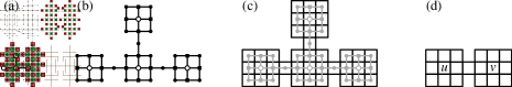
Figure 1: (a) The graph $G$ with prescribed angles between edges. The edges in the drawing have length 1. (b) The graph $H$ drawn with edges of length 1. (c) Representation of $H$ with unit squares. (d) Unique representation with unit squares of a subgraph of $H$ corresponding to an edge $uv$ in $G$.

Theorem 1

It is NP-complete to minimize the size of a pixel representation of a planar graph.

Proof: Clearly the corresponding decision problem is in NP, thus it remains to show NP-hardness. Let $G$ be a planar graph of maximum degree 4 and assume that the angles between adjacent edges are prescribed. We define a graph $H$ as follows (see Figs. 1a and  1b). First, replace every vertex by a wheel with five vertices such that the angles between the edges are respected. Second, subdivide every edge except those that are incident to the center of a wheel. We claim that $G$ admits a grid drawing with edges of length 1 (respecting the prescribed angles) if and only if $H$ admits a representation where every vertex is represented by exactly one pixel.

Assume $G$ admits a grid drawing with edges of length 1. Scaling the drawing by a factor of 4 and suitably adding the new vertices and edges clearly yields a drawing of $H$ with edges of length 1, such that two vertices have distance 1 only if they are adjacent; see Fig. 1b. For every vertex $v$ of $H$, we create a pixel $P_{v}$ with $v$ at its center (Fig. 1c). Clearly, for two adjacent vertices $u$ and $v$ in $H$, the pixels $P_{u}$ and $P_{v}$ touch as the edge $uv$ has length 1 in the drawing of $H$. Moreover, two pixel $P_{u}$ and $P_{v}$ touch only if $u$ and $v$ have distance 1 and thus only if $u$ and $v$ are adjacent. Hence, this set of pixels is a pixel representation of $H$.

Conversely, assume $H$ admits a representation such that every vertex $v$ is represented by a single pixel. Obviously, the subdivided wheel of size 4 has a unique representation (up to symmetries) consisting of a square of $3\times 3$ pixels. Consider two adjacent vertices $u$ and $v$ of $G$. Then there is a $3\times 3$ square for $u$ and one for $v$. As $u$ and $v$ adjacent in $G$, there must be a pixel representing the subdivision vertex on the edge $uv$ in $H$ that touches both $3\times 3$ squares (of $u$ and $v$) as in Fig. 1d. Thus, the straight line from the center of the square representing $u$ to the center of the square representing $v$ is either horizontal or vertical and has length 4. Hence, we obtain a drawing of $G$ where every edge has length 4. Scaling this drawing by a factor of ${1}/{4}$ yields a grid drawing of $G$ with edges of length 1. $\square$

Next, we reduce computing minimum-size pixel representations to computing minimum-size voxel representations.

Theorem 2

It is NP-complete to minimize the size of a voxel representation of a graph.

Proof: Again, the corresponding decision problem is clearly in NP. To show NP-hardness, we reduce from the 2D case. To this end, we build a rigid structure called cage that forces the graph in which we are actually interested to be drawn in a single plane.

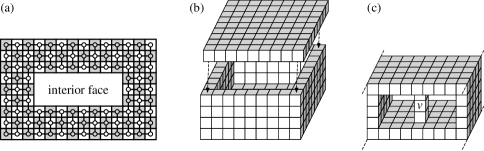
Figure 2: Illustration for the hardness proof in 3D. (a) A 2-dimensional cage with thickness $3$ and interior face of size $8\times 3$. (b) A 3-dimensional cage with thickness $1$ and interior of size $7\times 3\times 7$. (c) Attaching $v$ to two sides of the box forces it into interior of cage.

To simplify notation, we first prove for the 2-dimensional equivalent of a 3-dimensional cage that it actually is a rigid structure. We then extend this to 3D. The cage is basically the grid graph with a hole; see Fig. 2a. More precisely, the cage is defined by two parameters, the thickness $t$, which is an integer, and by the interior $w\times h$, which is a rectangle with integer width $w$ and integer height $h$. Given these parameters, the corresponding cage is the graph obtained from the $(2t+w)\times(2t+h)$ grid by deleting a $w\times h$ grid such that the distance from the external face to the large internal face corresponding to the interior is $t$. We call this internal face the interior face. Fig. 2a shows the cage with thickness $3$ and interior $8\times 3$ together with a contact representation with exactly one pixel per vertex.

Consider a pixel representation $\Gamma$ of the cage of thickness $t$ with interior $w\times h$. We show that either the bounding box of the interior face has size at most $w\times h$ or $\Gamma$ uses at least one pixel per vertex plus $t$ additional pixels. Thus, if we force some structure to lie in the interior of the cage, we can make the cost for using an area exceeding $w\times h$ arbitrarily large by increasing the thickness $t$ appropriately.

We partition the cage into cycles $C_{1},\dots,C_{t}$ where the vertices of $C_{i}$ have distance $i$ from the interior face. Consider $C_{1}$, which is the cycle bounding the interior face. The cycle $C_{1}$ has four corner vertices that are incident to two vertices in the outer face of $C_{1}$. All remaining vertices are incident to one vertex in the outer face. Requiring $C_{1}$ to be represented with exactly one pixel per vertex such that the corner vertices have two sides and every other vertex has one side incident to the outer face implies that $C_{1}$ must form a rectangle of size $(w+1)\times(h+1)$. Thus, if the bounding box of the interior face exceeds $w\times h$, $C_{1}$ requires at least one additional pixel. Moreover, the bounding box of the outer face of $C_{1}$ exceeds $(w+1)\times(h+1)$. Hence, an inductive argument shows that one requires at least one additional pixel for each of the cycles $C_{1},\dots,C_{t}$, which shows the above claim.

Analogously, we can build cages in 3D with thickness $t$ and interior $w\times h\times d$, by taking a 3D grid of size $(2t+w)\times(2t+h)\times(2t+d)$ and deleting a grid of size $w\times h\times d$. Fig. 2b shows the cage with $t=1$, and $w\times h\times d=7\times 3\times 7$. Assume that we have a graph $G$ for which we want to find an minimum-size pixel representation (in 2D). We build a 3D cage, choose $t$, $w$ and $d$ to be very large, and set $h=3$. To force $G$ to lie in the interior of the cage, we pick a vertex $v$ of $G$ and connect it to two vertices of the cage as shown in Fig. 2c. This forces $G$ to completely lie in the interior of the cage. As this interior has height $3$ and no vertex of $G$ (except for $v$) is allowed to touch another vertex of the cage, $G$ is forced to lie in a single plane when choosing $t$ sufficiently large (obviously, polynomial size is sufficient). Moreover, choosing $w$ and $d$ sufficiently large, ensures that the size of the plane available for $G$ does not restrict the possible representations of $G$. Finding a minimum-size pixel representation of $G$ is equivalent to finding a minimum-size voxel representation of the resulting graph $G^{\prime}$. $\square$

3 Lower and Upper Bounds in 2D

Here we only consider planar graphs since only planar graphs admit pixel representations. Let $G$ be a planar graph with fixed plane embedding $\mathcal{E}$. The embedding $\mathcal{E}$ is $1$-outerplane (or simply outerplane) if all vertices are on the outer face. It is $k$-outerplane if removing all vertices on the outer face yields a $(k-1)$-outerplane embedding. A graph $G$ is $k$-outerplanar if it admits a $k$-outerplane embedding but no $k^{\prime}$-outerplane embedding for $k^{\prime}<k$. Note that $k\in O(n)$, where $n$ is the number of vertices of $G$.

In Section 3.1, we show that pixel representations of an $n$-vertex $k$-outerplanar graph sometimes requires $\Omega(kn)$ pixels. As the number of pixels is a lower bound for the area consumption, this strengthens a result by Dolev et al. [21] that says that orthogonal drawings of planar graphs of maximum degree 4 and width $w$ sometimes require $\Omega(wn)$ area. As we will see later, width and $k$-outerplanarity are very similar concepts.

In Section 3.2, we show that $O(kn)$ area and thus using $O(kn)$ pixels is also sufficient. We use a result by Dolev et al. [21] who proved that any $n$-vertex planar graph of maximum degree 4 and width $w$ admits a planar orthogonal drawing of area $O(wn)$. The main difficulty is to extend their result to general planar graphs.

3.1 Lower Bound

Let $G$ be a $k$-outerplanar graph with a pixel representation $\Gamma$. Note that a pixel representation $\Gamma$ induces an embedding of $G$. Let $\Gamma$ induce a $k$-outerplane embedding of $G$, which we call a $k$-outerplane pixel representation for short. We claim that the width and the height of $\Gamma$ are at least $2k-1$. For $k=1$ this is trivial as every (non-empty) graph requires width and height at least $1$. For $k\geq 2$, let $V_{\mathrm{ext}}=\{v_{1},\dots,v_{\ell}\}$ be the set of vertices incident to the outer face of $\Gamma$. Removing $V_{\mathrm{ext}}$ from $G$ yields a $(k-1)$-outerplane graph $G^{\prime}$ with corresponding pixel representation $\Gamma^{\prime}$. By induction, $\Gamma^{\prime}$ requires width and height $2(k-1)-1$. As the representation of $V_{\mathrm{ext}}$ in $\Gamma$ encloses the whole representation $\Gamma^{\prime}$ in its interior, the width and the height of $\Gamma$ are at least two units larger than the width and the height of $\Gamma^{\prime}$, respectively.

Clearly, the number of pixels required by the vertices in $V_{\mathrm{ext}}$ is at least the perimeter of $\Gamma$ (twice the width plus twice the height minus 4 for the corners, which are shared) and thus at least $8k-8$. After removing the vertices in $V_{\mathrm{ext}}$, the new vertices on the outer face require $8(k-1)-8$ pixels, and so on. Thus, $\Gamma$ requires overall at least $\sum_{i=1}^{k}(8i-8)=4k^{2}-4k$ pixels, which gives the following lemma.

Lemma 3

Any $k$-outerplane pixel representation has size at least $4k^{2}-4k$.

There are $k$-outerplanar graphs with $n$ vertices such that $k\in\Theta(n)$. For example, the nested triangle graph with $2k$ triangles (see Fig. 4) has $n=6k$ vertices and is $k$-outerplanar for $k\geq 2$. Let $G$ be a graph with $c$ connected components each of which is $k$-outerplanar and has $\Theta(k)$ vertices. Then each connected component requires $4k^{2}-4k$ pixels (due to Lemma 3) and thus we need at least $(4k^{2}-4k)c$ pixels in total. As $G$ has $n=\Theta(kc)$ vertices, we get $(4k^{2}-4k)c\in\Theta(kn)$, which proves the following.

Theorem 4

Some $k$-outerplanar graphs require $\Omega(kn)$-size pixel representations.

3.2 Upper Bound

In the following two lemmas, we first show how to construct a pixel representation from a given orthogonal drawing and that taking minors does not heavily increase the number of pixels we need. Both lemmas aim at extending a result of Dolev et al. [21] on orthogonal drawings of planar graphs with maximum degree 4 to pixel representations of general planar graphs. As we re-use both lemmas in the 3D case (Section 4), we state them in the general $d$-dimensional setting.

Lemma 5

Let $G$ be a graph with $n$ vertices, $m$ edges, and an orthogonal drawing of total edge length $\ell$ in $d$-dimensional space. Then $G$ admits a $d$-dimensional representation of size $2\ell+n-m$.

Proof: We first scale the given drawing $\Gamma$ of $G$ by a factor of $2$ and subdivide the edges of $G$ such that every edge has length 1. Denote the resulting graph by $G^{\prime}$ and its drawing by $\Gamma^{\prime}$. An edge $e$ of length $\ell_{e}$ in $\Gamma$ is represented by a path with $2\ell_{e}-1$ internal vertices (the subdivision vertices). Thus, the total number of subdivision vertices is $2\ell-m$. Due to the scaling, non-adjacent vertices in $G^{\prime}$ have distance greater than 1 in $\Gamma^{\prime}$ (adjacent vertices have distance 1). Thus, representing every vertex $v$ by the box having $v$ as center yields a representation of $G^{\prime}$ with $2\ell+n-m$ boxes (one box per vertex of $G^{\prime}$). If we assign the boxes representing subdivision vertices to one of the endpoints of the corresponding edge, we get a representation of $G$ with $2\ell+n-m$ boxes. $\square$

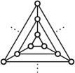
Figure 3: A nested triangle graph of outerplanarity $\Omega(n)$.

(a)	(b)	(c)

Figure 4: Constructing a representation of a minor with asymptotically the same number of blocks.

Lemma 6

Let $G$ be a graph that has a $d$-dimensional representation of size $b$. Every minor of $G$ admits a $d$-dimensional representation of size at most $3^{d}b$.

Proof: Let $H$ be a minor obtained from $G$ by first deleting some edges, then deleting isolated vertices, and finally contracting edges. We start with the representation $\Gamma$ of $G$ using $b$ boxes and scale it by a factor of 3. This yields a representation $3\Gamma$ using $3^{d}b$ boxes. Then we modify $3\Gamma$, without adding boxes, to represent the minor $H$. For convenience, we consider the 2D case; the case $d>2$ works analogously.

Let $uv$ be an edge in $G$ that is deleted. In $3\Gamma$ we delete every pixel in the representation of $u$ that touches a pixel of the representation of $v$. We claim that this neither destroys the contact of $u$ with any other vertex nor does it disconnect the shape representing $u$. Consider a single pixel $B$ in $\Gamma$. In $3\Gamma$ it is represented by a square of $3\times 3$ pixels belonging to $B$. If $B$ is in contact to another pixel $A$ in $\Gamma$, then there is a pair of pixels $A^{\prime}$ and $B^{\prime}$ in $3\Gamma$ such that $A^{\prime}$ and $B^{\prime}$ are in contact, while all other pixels that touch $A^{\prime}$ and $B^{\prime}$ belong to $A$ and $B$, respectively; see Figs. 4a and 4b. Assume that we remove in $3\Gamma$ all pixels belonging to $B$ that are in contact to pixels belonging to another pixel $C$ touching $B$ in $\Gamma$; see Fig. 4c. Obviously, this does not effect the contact between $A^{\prime}$ and $B^{\prime}$. Moreover, the remaining pixels belonging to $B$ form a connected blob. The above claim follows immediately.

Removing isolated vertices can be done by simply removing their representation. Moreover, contracting an edge $uv$ into a vertex $w$ can be done by merging the blobs representing $u$ and $v$ into a single blob representing $w$. This blob is obviously connected and touches the blob of another vertex if and only if either $u$ or $v$ touch this vertex. $\square$

Now let $G$ be a $k$-outerplanar graph. Applying the algorithm of Dolev et al. [21] yields an orthogonal drawing of total length $O(wn)$, where $w$ is the width of $G$. The width $w$ of $G$ is the maximum number of vertices contained in a shortest path from an arbitrary vertex of $G$ to a vertex on the outer face. Given the orthogonal drawing, Lemma 5 gives us a pixel representation of $G$. There are, however, two issues. First, $k$ and $w$ are not the same (e.g., subdividing edges increases $w$ but not $k$). Second, $G$ does not have maximum degree 4, thus we cannot simply apply the algorithm of Dolev et al. [21].

Concerning the first issue, we note that the algorithm of Dolev et al. exploits that $G$ has width $w$ only to find a special type of separator [21, Theorem 1]. For this, it is sufficient that $G$ is a subgraph of a graph of width $w$ (not necessarily with maximum degree 4; in fact Dolev et al. triangulate the graph before finding the separator).

Lemma 7

Every $k$-outerplanar graph has a planar supergraph of width $w=k$.

Proof: Let $G$ be a graph with a $k$-outerplane embedding. Iteratively deleting the vertices on the outer face gives us a sequence of deletion phases. For each vertex $v$, let $k_{v}$ be the phase in which $v$ is deleted. Note that the maximum over all values of $k_{v}$ is exactly $k$. For any vertex $v$, either $k_{v}=1$ or there is a vertex $u$ with $k_{u}=k_{v}-1$ such that $u$ and $v$ are incident to a common face. Thus, there is a sequence $v_{1},\dots,v_{k_{v}}$ of $k_{v}$ vertices such that (i) $v_{1}=v$, (ii) $v_{k_{v}}$ lies on the outer face, and (iii) $v_{i}$, $v_{i+1}$ are incident to a common face. If the graph $G$ was triangulated, this would yield a path containing $k_{v}$ vertices from $v$ to a vertex on the outer face. Thus, triangulated $k$-outerplanar graphs have width $w=k$.

It remains to show that $G$ can be triangulated without increasing $k_{v}$ for any vertex $v$. Consider a face $f$ and let $u$ be the vertex incident to $f$ for which $k_{u}$ is minimal. Let $v\not=u$ be any other vertex incident to $f$. Adding the edge $uv$ clearly does not increase the value $k_{x}$ for any vertex $x$. We add edges in this way until the graph is triangulated. Alternatively, we can use a result of Biedl [7] to triangulate $G$. Note that we do not need to triangulate the outer face of $G$. Hence, we do not increase the outerplanarity. $\square$

To solve the second issue (the $k$-outerplanar graph $G$ not having maximum degree 4), we construct a graph $G^{\prime}$ such that $G$ is a minor of $G^{\prime}$, $G^{\prime}$ is $k$-outerplanar, and $G^{\prime}$ has maximum degree 4. Then, (due to Lemma 7) we can apply the algorithm of Dolev et al. [21] to $G^{\prime}$. Next, we apply Lemma 5 to the resulting drawing to get a representation of $G^{\prime}$ with $O(kn)$ pixels. As $G$ is a minor of $G^{\prime}$, Lemma 6 yields a representation of $G$ that, too, requires $O(kn)$ pixels.

Theorem 8

Every $k$-outerplanar $n$-vertex graph has a size $O(kn)$ pixel representation.

Proof: Let $G$ be a $k$-outerplanar graph. After the above considerations, it remains to construct a $k$-outerplanar graph $G^{\prime}$ with maximum degree 4 such that $G$ is a minor of $G^{\prime}$. Let $u$ be a vertex with $\deg(u)>4$. We replace $u$ with a path of length $\deg(u)$ and connect each neighbor of $u$ to a unique vertex of this path. This can be done maintaining a plane embedding. We now show that the resulting graph remains $k$-outerplanar.

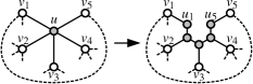
Figure 5: Replacement of high-degree vertices while preserving $k$-outerplanarity.

Consider a vertex $u$ on the outer face with neighbors $v_{1},\dots,v_{\ell}$. Assume the neighbors appear in that order around $u$ such that $v_{1}$ is the counter-clockwise successor of $u$ on the outer face; see Fig. 5. We replace $u$ with the path $u_{1},\dots,u_{\ell}$ and connect $u_{i}$ to $v_{i}$ for $1\leq i\leq\ell$. Call the resulting graph $G_{u}$. Note that all $u_{i}$ in $G_{u}$ are incident to the outer face. Thus, if $G$ was $k$-outerplanar, $G_{u}$ is also $k$-outerplanar. Moreover, the degrees of the new vertices do not exceed 4 (actually not even 3), and $G$ is a minor of $G_{u}$—one can simply contract the inserted path to obtain $G$.

We can basically apply the same replacement if $u$ is not incident to the outer face. Assume that we delete $u$ in phase $k_{u}$ if we iteratively delete vertices incident to the outer face. When replacing $u$ with the vertices $u_{1},\dots,u_{\ell}$, we have to make sure that all these vertices get deleted in phase $k_{u}$. Let $f$ be a face incident to $u$ that is merged with the outer face after $k_{u}-1$ deletion phases (such a face must exist, otherwise $u$ is not deleted in phase $k_{u}$). We apply the same replacement as for the case where $u$ was incident to the outer face, but this time we ensure that the new vertices $u_{i}$ are incident to the face $f$. Thus, after $k_{u}-1$ deletion phases they are all incident to the outer face and thus they are deleted in phase $k_{u}$. Hence, the resulting graph $G_{u}$ is $k$-outerplanar. Again the new vertices have degree at most 3 and $G$ is obviously a minor of $G_{u}$. Iteratively applying this kind of replacement for ever vertex $u$ with $\deg(u)>4$ yields the claimed graph $G^{\prime}$.

The corresponding drawing can then be obtained as follows. Since $G^{\prime}$ has a supergraph of width $w=k$ by Lemma 7, and $G^{\prime}$ has maximum degree 4, we use the algorithm of Dolev et al. [21] to obtain a drawing of $G^{\prime}$ with area (and hence total edge length) $O(nk)$. By Lemma 5, we thus obtain a representation of $G^{\prime}$ with $O(nk)$ pixels. Since $G$ is a minor of $G^{\prime}$, Lemma 6 yields a representation of $G$ with $O(nk)$ pixels. $\square$

4 Representations in 3D

In this section, we consider voxel representations. We start with some basic considerations showing that every $n$-vertex graph admits a representation with $O(n^{2})$ voxels. Note that $\Omega(n^{2})$ is obviously necessary for $K_{n}$ as every edge corresponds to a face-to-face contact and every voxel has at most $6$ such contacts. We improve on this simple general result in two ways. First, we show that $n$-vertex graphs with treewidth at most $\tau$ admit voxel representations of size $O(n\cdot\tau)$ (see Section 4.1). Second, for $n$-vertex graphs with genus at most $g$, we obtain representations with $O(g^{2}n\log^{2}n)$ voxels (see Section 4.2).

Theorem 9

Any $n$-vertex graph admits a voxel representation of size $O(n^{2})$.

Proof: Let $G$ be a graph with vertices $v_{1},\dots,v_{n}$. Vertex $v_{i}$ ($i=1,\dots,n$) is represented by three cuboids (see Fig. 6a), namely a vertical cuboid consisting of the voxels centered at the points $(2i,2,0),(2i,3,0),\dots,(2i,2n,0)$, a horizontal cuboid consisting of the voxels centered at $(2,2i,2),(3,2i,2),\dots,(2n,2i,2)$, and the voxel centered at $(2i,2i,1)$. This yields a representation where every vertex is a connected blob and no two blobs are in contact. Moreover, for every pair of vertices $v_{i}$ and $v_{j}$, there is a voxel of $v_{i}$ at $(2i,2j,0)$ and a voxel of $v_{j}$ at $(2i,2j,2)$ and no voxel between them at $(2i,2j,1)$. Thus, one can easily represent an arbitrary edge $(v_{i},v_{j})$ by extending the representation of $v_{i}$ to also contain $(2i,2j,1)$; see Fig. 6b. Clearly, this representation consists of $O(n^{2})$ voxels. $\square$

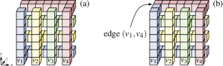
Figure 6: (a) The basic contact representation without any contacts between vertices. (b) If $v_{1}$ and $v_{4}$ are adjacent, it suffices to add a single voxel to the representation of $v_{1}$ (or to that of $v_{4}$).

4.1 Graphs of Bounded Treewidth

Let $G=(V,E)$ be a graph. A tree decomposition of $G$ is a tree $T$ where each node $\mu$ in $T$ is associated with a bag $X_{\mu}\subseteq V$ such that: (i) for each $v\in V$, the nodes of $T$ whose bags contain $v$ form a connected subtree, and (ii) for each edge $uv\in E$, $T$ contains a node $\mu$ such that $u,v\in X_{\mu}$.

Note that we use (lower case) Greek letters for the nodes of $T$ to distinguish them from the vertices of $G$. The width of the tree decomposition is the maximum bag size minus $1$. The treewidth of $G$ is the minimum width over all tree decompositions of $G$. A tree decomposition is nice if $T$ is a rooted binary tree, where for every node $\mu$:

• $\mu$ is a leaf and $|X_{\mu}|=1$ (leaf node), or

• $\mu$ has a single child $\eta$ with $X_{\mu}\subseteq X_{\eta}$ and $|X_{\mu}|=|X_{\eta}|-1$ (forget node), or

• $\mu$ has a single child $\eta$ with $X_{\eta}\subseteq X_{\mu}$ and $|X_{\mu}|=|X_{\eta}|+1$ (introduce node), or

• $\mu$ has two children $\eta$ and $\kappa$ with $X_{\mu}=X_{\eta}=X_{\kappa}$ (join node).

Any tree decomposition can be transformed (without increasing its width) into a nice tree decomposition such that the resulting tree $T$ has $O(n)$ nodes, where $n$ is the number of vertices of $G$ [9]. This transformation can be done in linear time. Thus, we can assume any tree decomposition to be a nice tree decomposition with a tree of size $O(n)$.

Lemma 10

Let $T$ be a nice tree decomposition of a graph $G$. The edges of $G$ can be mapped to the nodes of $T$ such that every edge $uv$ of $G$ is mapped to a node $\mu$ with $u,v\in X_{\mu}$ and the edges mapped to each node $\mu$ form a star.

Proof: We say that a node $\mu$ represents the edge $uv$ if $uv$ is mapped to $\mu$. Consider a node $\mu$ during a bottom-up traversal of $T$. We want to maintain the invariant that, after processing $\mu$, all edges between vertices in $X_{\mu}$ are represented by $\mu$ or by a descendant of $\mu$. This ensures that every edge is represented by at least one node. Every edge can then be mapped to one of the nodes representing it.

If $\mu$ is a leaf, it cannot represent an edge as $|X_{\mu}|=1$. If $\mu$ is a forget node, it has a child $\eta$ with $X_{\mu}\subseteq X_{\eta}$. Thus, by induction, all edges between vertices in $X_{\mu}$ are already represented by descendants of $\mu$. If $\mu$ is an introduce node, it has a child $\eta$ and $X_{\mu}=X_{\eta}\cup\{u\}$ for a vertex $u$ of $G$. By induction, all edges between nodes in $X_{\eta}$ are already represented by descendants of $\mu$. Thus, $\mu$ only needs to represent the edges between the new node $u$ and other nodes in $X_{\mu}$. Note that these edges form a star with center $u$. Finally, if $\mu$ is a join node, no edge needs to be represented by $\mu$ (by the same argument as for forget nodes). This concludes the proof. $\square$

We obtain a small voxel representation roughly as follows. We start with a “2D” voxel representation of the tree $T$, that is, all voxel centers lie in the $x$–$y$ plane. We take $\tau+1$ copies of this representation and place them in different layers in 3D space. We then assign to each vertex $v$ of $G$ a piece of this layered representation such that its piece contains all nodes of $T$ that include $v$ in their bags. For an edge $uv$, let $\mu$ be the node to which $uv$ is mapped by Lemma 10. By construction, the representation of $\mu$ occurs multiple times representing $u$ and $v$ in different layers. To represent $uv$, we only have to connect the representations of $u$ and $v$. As it suffices to represent a star for each node $\mu$ in this way, the number of voxels additionally used for these connections is small.

Theorem 11

Any $n$-vertex graph of treewidth $\tau$ has a voxel representation of size $O(n\tau)$.

Proof: Let $G$ be an $n$-vertex graph of treewidth $\tau$. During our construction, we will get some contacts between the blobs of vertices that are actually not adjacent in $G$. As $G$ is a minor of the graph that we represent this way, we can use Lemma 6 to get a representation of $G$. Let $T$ be a nice tree decomposition of $G$. As a tree, $T$ is outerplanar and, hence, admits a pixel representation $\Gamma$ with $O(n)$ pixels (by Theorem 8). Let $\Gamma_{1},\dots,\Gamma_{k}$ be voxel representations corresponding to $\Gamma$ with $z$-coordinates $1,\dots,k=\tau+1$.

For a vertex $v$ of $G$, we denote by $\Gamma_{i}(v)$ the sub-representation of $\Gamma_{i}$ induced by the nodes of $T$ whose bags contain $v$. Now let $c\colon V\to\{1,\dots,k\}$ be a $k$-coloring of $G$ with color set $\{1,\dots,k\}$ such that no two vertices sharing a bag have the same color. Such a coloring can be computed by traversing $T$ bottom up, assigning in every introduce node $\mu$ a color to the new vertex that is not already used by any other vertex in $X_{\mu}$. As a basis for our construction, we represent each vertex $v$ of $G$ by the sub-representation $\Gamma_{c(v)}(v)$.

So far, we did not represent any edge of $G$. Our construction, however, has the following properties: (i) it uses $O(nk)$ voxels. (ii) every vertex is a connected set of voxels. (iii) for every node $\mu$ of $T$, there is a position $(x_{\mu},y_{\mu})$ in the plane such that, for every vertex $v\in X_{\mu}$, the voxel at $(x_{\mu},y_{\mu},c(v))$ belongs to the representation of $v$. Scaling the representation by a factor of $2$ ensures that this is not the only voxel for $v$ and that $v$ is not disconnected if this voxel is removed (or reassigned to another vertex).

By Lemma 10 it suffices to represent for every node $\mu$ edges between vertices in $X_{\mu}$ that form a star. Let $u$ be the center of this star. We simply assign the voxels centered at $(x_{\mu},y_{\mu},1),\dots,(x_{\mu},y_{\mu},k)$ to the blob of $u$. This creates a contact between $u$ and every other vertex $v\in X_{\mu}$ (by the above property that the voxel $(x_{\mu},y_{\mu},c(v))$ belonged to $v$ before). Finally, we apply Lemma 6 to get rid of unwanted contacts. The resulting representation uses $O(nk)$ voxels, which concludes the proof. $\square$

Note that cliques of size $k$ require $\Omega(k^{2})$ voxels. Taking the disjoint union of $n/k$ such cliques yields graphs with $n$ vertices requiring $\Omega(nk)$ voxels. Note that these graphs have treewidth $\tau=k-1$. Thus, the bound of Theorem 11 is asymptotically tight.

Theorem 12

Some $n$-vertex graphs of treewidth $\tau$ require $\Omega(n\tau)$ voxels.

4.2 Graphs of Bounded Genus

Since planar graphs (genus $0$) have treewidth $O(\sqrt{n})$ [28], we can obtain a voxel representation of size $O(n^{1.5})$ for any planar graph, from Theorem 11. Next, we improve this bound to $O(n\log^{2}n)$ by proving a more general result for graphs of bounded genus. Recall that we used known results on orthogonal drawings with small area to obtain small pixel representations in Section 3.2. Here we follow a similar approach (re-using Lemmas 5 and 6), now allowing the orthogonal drawing we start with to be non-planar.

We obtain small voxel representations by first showing that it is sufficient to consider graphs of maximum degree 4: we replace higher-degree vertices by connected subgraphs as in the proof of Theorem 8. Then we use a result of Leiserson [32] who showed that any graph of genus $g$ and maximum degree 4 admits a 2D orthogonal drawing of area $O((g+1)^{2}n\log^{2}n)$, possibly with edge crossings. The area of an orthogonal drawing is clearly an upper bound for its total edge length. Finally we turn the pixels into voxels and use the third dimension to get rid of the crossings without using too many additional voxels.

Theorem 13

Every $n$-vertex graph of genus $g$ admits a voxel representation of size $O((g+1)^{2}n\log^{2}n)$.

Proof: Let $G$ be an $n$-vertex graph, and let $u$ be a vertex of degree $\ell>4$. Assume $G$ to be embedded on a surface of genus $g$, and let $v_{1},\dots,v_{\ell}$ be the neighbors of $u$ appearing in that order around $u$ (with respect to the embedding). We replace $u$ with the cycle $u_{1},\dots,u_{\ell}$ and connect $u_{i}$ to $v_{i}$ for $1\leq i\leq\ell$; see Fig. 7a. Clearly, the new vertices have degree 3 and the genus of the graph has not increased. Applying this modification to every vertex of degree at least 5 yields a graph $G_{4}$ of maximum degree 4 and genus $g$. Moreover, $G$ is a minor of $G_{4}$ as one can undo the cycle replacements by contracting all edges in the cycles. Thus, we can transform a voxel representation of $G_{4}$ into a voxel representation of $G$ by applying Lemma 6.

We claim that the number $n_{4}$ of vertices in $G_{4}$ is linear in $n$. Indeed, if $m$ denotes the number of edges in $G$, then we have $n_{4}\leq n+2m$. Moreover, we can assume without loss of generality that $g\in O(n)$ (otherwise Theorem 9 already gives a better bound). This implies that $m\in O(n)$ and hence, $n_{4}\in O(n)$, as we claimed.

We thus assume that $G$ has maximum degree 4. Then $G$ has a (possibly non-planar) orthogonal drawing $\Gamma$ of total edge length $O(g^{2}n\log^{2}n)$ [32]. We modify $G$ and $\Gamma$ as follows. For every bend on an edge $e$ in $\Gamma$, we subdivide the edge $e$ once yielding a partition of the edges of the subdivided graph into horizontal and vertical edges. We obtain a graph $G^{\prime}$ from this subdivision of $G$ by replacing every vertex $v$ by two adjacent vertices $v_{1}$ and $v_{2}$, and connecting $v_{1}$ and $w_{1}$ (respectively $v_{2}$ and $w_{2}$) by an edge if $v$ and $w$ are connected by a horizontal (respectively vertical edge); see Fig. 7b.

Figure 7: Constructing voxel representations for bounded-genus graphs: (a) replacing high-degree vertices while preserving the genus, (b) subdividing and decomposing a graph according to a non-planar orthogonal drawing with small area, and (c) constructing a 3D drawing with small total edge length from the decomposition in (b).

We draw $G^{\prime}$ in 3D space by using the drawing $\Gamma$ and setting for every vertex $v$ the $z$-coordinate of $v_{1}$ and $v_{2}$ to $0$ and $1$, respectively. The $x$- and $y$-coordinates of vertices and edges are the same as in $\Gamma$; see Fig. 7b. Note that $G$ is a minor of $G^{\prime}$: we obtain $G$ from $G^{\prime}$ by contracting (i) the edge $v_{0}v_{1}$ for every vertex $v$ and (ii) any subdivision vertex. Asymptotically, the total edge length of $\Gamma^{\prime}$ is the same as that of $\Gamma$, that is, $O((g+1)^{2}n\log^{2}n)$. By Lemma 5, we turn $\Gamma^{\prime}$ into a voxel representation of $G^{\prime}$ and, by Lemma 6, into a voxel representation of $G$ with size $O((g+1)^{2}n\log^{2}n)$. $\square$

5 Conclusion

In this paper, we have studied pixel representations and voxel representations of graphs, where vertices are represented by disjoint blobs (that is, connected sets of grid cells) and edges correspond to pairs of blobs with face-to-face contact. We have shown that it is NP-complete to minimize the number of pixels or voxels in such representations. Does this problem admit an approximation algorithm?

We have shown that $O((g+1)^{2}n\log^{2}n)$ voxels suffice for any $n$-vertex graph of genus $g$. It remains open to improve this upper bound or to give a non-trivial lower bound. We believe that any planar graph admits a voxel representation of linear size.

References

- [1] N. Aerts and S. Felsner. Vertex contact graphs of paths on a grid. In Graph-Theoretic Concepts Comput. Sci. (WG’14), volume 8747, pages 56–68, 2014.
- [2] M. J. Alam, T. Biedl, S. Felsner, M. Kaufmann, S. Kobourov, and T. Ueckerdt. Computing cartograms with optimal complexity. Discrete Comput. Geom., 50(3):784–810, 2013.
- [3] M. Badent, C. Binucci, E. D. Giacomo, W. Didimo, S. Felsner, F. Giordano, J. Kratochvíl, P. Palladino, M. Patrignani, and F. Trotta. Homothetic triangle contact representations of planar graphs. In Canad. Conf. Comput. Geom. (CCCG’07), pages 233–236, 2007.
- [4] A. Bezdek. On the number of mutually touching cylinders. Comb. Comput. Geom., 52:121–127, 2005.
- [5] K. Bezdek and S. Reid. Contact graphs of unit sphere packings revisited. J. Geom., 104(1):57–83, 2013.
- [6] S. N. Bhatt and S. S. Cosmadakis. The complexity of minimizing wire lengths in VLSI layouts. Inf. Process. Lett., 25(4):263–267, 1987.
- [7] T. Biedl. On triangulating -outerplanar graphs. CoRR, abs/1310.1845, 2013.
- [8] T. C. Biedl. Small drawings of outerplanar graphs, series-parallel graphs, and other planar graphs. Discrete Comput. Geom., 45(1):141–160, 2011.
- [9] H. L. Bodlaender. Treewidth: Algorithmic techniques and results. In Math. Foundat. Comput. Sci. (MFCS’97), volume 1295, pages 19–36, 1997.
- [10] P. Bose, H. Everett, S. P. Fekete, M. E. Houle, A. Lubiw, H. Meijer, K. Romanik, G. Rote, T. C. Shermer, S. Whitesides, and C. Zelle. A visibility representation for graphs in three dimensions. J. Graph Algorithms Appl., 2(2), 1998.
- [11] F. Brandenburg, D. Eppstein, M. Goodrich, S. Kobourov, G. Liotta, and P. Mutzel. Selected open problems in graph drawing. In Graph Drawing (GD’03), volume 2912, pages 515–539, 2003.
- [12] F. J. Brandenburg. 1-visibility representations of 1-planar graphs. J. Graph Algorithms Appl., 18(3):421–438, 2014.
- [13] D. Bremner, W. S. Evans, F. Frati, L. J. Heyer, S. G. Kobourov, W. J. Lenhart, G. Liotta, D. Rappaport, and S. Whitesides. On representing graphs by touching cuboids. In Graph Drawing (GD’12), volume 7704, pages 187–198, 2012.
- [14] A. L. Buchsbaum, E. R. Gansner, C. M. Procopiuc, and S. Venkatasubramanian. Rectangular layouts and contact graphs. ACM Transactions on Algorithms, 4(1), 2008.
- [15] T. M. Chan, M. T. Goodrich, S. R. Kosaraju, and R. Tamassia. Optimizing area and aspect ratio in straight-line orthogonal tree drawings. 23(2):153–162, 2002.
- [16] S. Chaplick, S. G. Kobourov, and T. Ueckerdt. Equilateral L-contact graphs. In Graph-Theoretic Concepts Comput. Sci. (WG’13), volume 8165, pages 139–151, 2013.
- [17] H. de Fraysseix and P. O. de Mendez. Representations by contact and intersection of segments. Algorithmica, 47(4):453–463, 2007.
- [18] H. de Fraysseix, P. O. de Mendez, and P. Rosenstiehl. On triangle contact graphs. Comb. Prob. Comput., 3:233–246, 1994.
- [19] H. de Fraysseix, J. Pach, and R. Pollack. How to draw a planar graph on a grid. Combinatorica, 10(1):41–51, 1990.
- [20] G. Di Battista and F. Frati. Small area drawings of outerplanar graphs. Algorithmica, 54(1):25–53, 2009.
- [21] D. Dolev, T. Leighton, and H. Trickey. Planar embedding of planar graphs. Adv. Comput. Research, 2:147–161, 1984.
- [22] V. Dujmović, P. Morin, and D. Wood. Layered separators for queue layouts, 3d graph drawing and nonrepetitive coloring. In Foundat. Comput. Sci. (FOCS’13), pages 280–289, 2013.
- [23] C. A. Duncan, E. R. Gansner, Y. F. Hu, M. Kaufmann, and S. G. Kobourov. Optimal polygonal representation of planar graphs. Algorithmica, 63(3):672–691, 2012.
- [24] W. Evans, M. Kaufmann, W. Lenhart, T. Mchedlidze, and S. Wismath. Bar 1-visibility graphs and their relation to other nearly planar graphs. 18(5):721–739, 2014.
- [25] J. Fan, C. Lin, H. Lu, and H. Yen. Width-optimal visibility representations of plane graphs. In Int. Symp. Algorithms Comput. (ISAAC’07), volume 4835, pages 160–171, 2007.
- [26] S. Felsner. Rectangle and square representations of planar graphs. Thirty Essays on Geometric Graph Theory, pages 213–248, 2013.
- [27] S. Felsner and M. C. Francis. Contact representations of planar graphs with cubes. In Symp. Comput. Geom. (SoCG’11), pages 315–320, 2011.
- [28] F. V. Fomin and D. M. Thilikos. New upper bounds on the decomposability of planar graphs. 51(1):53–81, 2006.
- [29] P. Hliněný. Classes and recognition of curve contact graphs. J. Comb. Theory B, 74(1):87–103, 1998.
- [30] P. Hliněný and J. Kratochvíl. Representing graphs by disks and balls (a survey of recognition-complexity results). Discrete Math., 229(1–3):101–124, 2001.
- [31] P. Koebe. Kontaktprobleme der konformen Abbildung. Berichte über die Verhandlungen der Sächsischen Akademie der Wissenschaften zu Leipzig. Math.-Phy. Kla., 88:141–164, 1936.
- [32] C. E. Leiserson. Area-efficient graph layouts (for VLSI). In Foundat. Comput. Sci. (FOCS’80), pages 270–281, 1980.
- [33] J. Pach, T. Thiele, and G. Tóth. Three-dimensional grid drawings of graphs. In Graph Drawing (GD’97), volume 1353, pages 47–51, 1997.
- [34] M. Patrignani. Complexity results for three-dimensional orthogonal graph drawing. 6(1):140–161, 2008.
- [35] W. Schnyder. Embedding planar graphs on the grid. In Symp. Discrete Algorithms (SODA’90), pages 138–148, 1990.
- [36] R. Tamassia and I. G. Tollis. A unified approach a visibility representation of planar graphs. Discrete Comput. Geom., 1:321–341, 1986.
- [37] C. Thomassen. Interval representations of planar graphs. J. Comb. Theory B, 40(1):9–20, 1986.
- [38] C. Zong. The kissing numbers of tetrahedra. Discrete Comput. Geom., 15(3):239–252, 1996.