ExoMol molecular line lists XII: Line Lists for 8 isotopologues of CS

Abstract

Comprehensive vibration-rotation line lists for eight isotopologues of carbon monosulphide (CS) (¹²C³²S, ¹²C³³S, ¹²C³⁴S, ¹²C³⁶S, ¹³C³²S, ¹³C³³S, ¹³C³⁴S, ¹³C³⁶S) in their ground electronic states are calculated. These line lists are suitable for temperatures up to 3000 K. A spectroscopically-determined potential energy curve (PEC) and dipole moment curve (DMC) are taken from literature. This PEC is adapted to suit our method prior to the computation of ro-vibrational energies. The calculated energies are then substituted by experimental energies, where available, to improve the accuracy of the line lists. The ab initio DMC is used without refinement to generate Einstein A coefficients. Full line lists of vibration-rotation transitions and partition functions are made available in an electronic form as supporting information to this paper and at www.exomol.com.

molecular data; opacity; astronomical data bases: miscellaneous; planets and satellites: atmospheres; stars: low-mass

1 Introduction

It was the development of radio astronomy that led to the realisation that the majority of our galaxy, and hence the universe, is dominated by molecular processes. More than 150 molecules have been detected so far in the interstellar medium (ISM) by direct observation of their spectra. Carbon monosulphide (CS) is one of these molecules (Penzias et al., 1971) and is a diatomic of both atmospheric as well as astrophysical interest. In the Earth’s atmosphere, CS plays a role in the formation of aerosols, in particular carbonyl sulphide (OCS) in the troposphere (Li et al., 2013).

In the solar system CS has been observed in comets (Canaves et al., 2007) and the collision of comet Shoemaker-Levy 9 (Orton et al., 1995) led to its detection in the atmosphere of Jupiter (Moreno et al., 2003). Astronomically the molecule has been observed in a variety of objects such as carbon-rich stars (Bregman et al., 1978; Botschwina & Sebald, 1985; Agundez & Cernicharo, 2006), star forming regions (Davis et al., 2013) and dense interstellar clouds (Nilsson et al., 2000; McQuinn et al., 2002; Scoville et al., 2015). In fact CS is one of the most abundant sulphur-containing species in interstellar clouds (Shi et al., 2011; Bilalbegovic & Baranovic, 2015) with several isotopologues long detected outside the Milky Way (Henkel & Bally, 1985; Mauersberger et al., 1989b, a; Henkel et al., 1993).

The numerous astronomical detections of CS and the importance of the molecule in our own atmosphere has motivated copious laboratory studies. Experimentally the CS spectrum has been studied in wavelength regions ranging from the microwave to the ultraviolet (UV). A pioneering study was carried out by Crawford & Shurcliff (1934) whom discovered the main $A~{}^{1}\Pi$ - $X~{}^{1}\Sigma^{+}$ transition in the visible. Additional electronic transitions in the visible to near UV have been investigated by, for example, Bell et al. (1972), Cossart et al. (1977) and Stark et al. (1987).

Mockler & Bird (1955) made the first measurements of rotational lines for the ¹²C³²S, ¹²C³³S, ¹²C³⁴S and ¹³C³²S isotopomers in the microwave region. Transitions in this region have also been observed by, for example, Lovas & Krupenie (1974). Early work in the millimetre wave region began with measurements of rotational ¹²C³²S and ¹²C³⁴S lines by Kewley et al. (1963), later extended by Bogey et al. (1982) who additionally observed ¹³C³²S. Bogey et al. (1981) also presented a study of the millimetre spectrum of rarer isotopologues ¹²C³³S,¹²C³⁶S, ¹³C³³S and ¹³C³⁴S. More recent work in the region has been carried out by Ahrens & Winnewisser (1999) (¹²C³²S, ¹²C³⁴S, ¹²C³³S, ¹³C³²S, ¹²C³⁶S, ¹³C³³S, ¹³C³⁴S), Kim & Yamamoto (2003) (¹²C³²S, ¹²C³⁴S) and Gottlieb et al. (2003) (¹²C³²S, ¹²C³⁴S, ¹²C³³S, ¹³C³²S).

The first study in the infra-red region was performed by Todd (1977) who measured the $v=2-0$ vibrational band of the main isotope while Todd & Olson (1979) and Yamada & Hirota (1979) measured several $\Delta v$ = 1 bands of ¹²C³²S, ¹²C³³S, ¹²C³⁴S and ¹³C³²S. The resulting molecular parameters were later refined by Winkel et al. (1984) and Burkholder et al. (1987). Winkel et al. (1984) measured many $\Delta v$ = 2 bands for vibrational levels up to $v$ = 8 while Burkholder et al. (1987) obtained high resolution measurements of the 1-0 band, and 2-1 band for the main isotope, of ¹²C³³S, ¹²C³⁴S and ¹³C³²S for $J$ up to 41, 28, 32 and 28 respectively. $\Delta v$ = 1 bands up to $v$ = 9-8 for the main isotope were later measured by Ram et al. (1995). The most recent research on CS infra-red spectra has been performed by Uehara et al. (2015), who reported $\Delta v$ = 1 transitions of ¹³C³²S up to $v$ = 5-4. Additionally they measured $\Delta v$ = 1 transitions of ¹²C³²S up to $v$ = 7-6 to a higher accuracy than Ram et al. (1995).

Using the vibration-rotation and pure rotation data on this molecule available to them, Coxon & Hajigeorgiou (1992) derived a spectroscopic potential energy curve (PEC) that reproduced all the input experimental data within experimental error. This PEC is the starting point for the current work.

Transition probabilities or Einstein A coefficients have been provided by Botschwina & Sebald (1985) and Pineiro et al. (1987). The latter produced transition lists for rotational quantum numbers $J^{\prime}-J=\pm 1$ for $J\leq 200$, and vibrational $v\leq 20$, though only for the four most abundant isotopes (¹²C³²S, ¹²C³³S, ¹²C³⁴S and ¹³C³²S). Line lists for all isotopologues of CS, including some rotation-vibration transitions, are available from CDMS (Müller et al., 2005). These were constructed from experimental data obtained by Bogey et al. (1982), Bogey et al. (1981), Ahrens & Winnewisser (1999), Kim & Yamamoto (2003) , Gottlieb et al. (2003), Burkholder et al. (1987), Ram et al. (1995), Winkel et al. (1984) and the only available experimental measurements of the dipole moment (Winnewisser & Cook, 1968). The line lists are very accurate and recommended for use in radio astronomy, though are limited to $v\leq 4$ and $J\leq 99$ and hence temperatures, $T$ below about 500 K. The aim of this work is to produce comprehensive line lists for all stable isotopologues of CS suitable for modelling hot environments, such as carbon stars ($T\sim 3000$ K).

The ExoMol project aims to provide line lists on all the molecular transitions of importance in the atmospheres of planets (Tennyson & Yurchenko, 2012). The ExoMol methology has already been applied to a number of diatomic molecules: BeH, MgH and CaH (Yadin et al., 2012), SiO (Barton et al., 2013), NaCl and KCl (Barton et al., 2014), PN (Yorke et al., 2014), AlO (Patrascu et al., 2015) and NaH (Rivlin et al., 2015). In this paper, we present ro-vibrational transition lists and associated spectra for all stable isotopologues of CS.

2 Method

The line lists for all eight isotopologues of CS, which we have named JnK, were obtained by solving the Schrödinger equation allowing for Born-Oppenheimer Breakdown (BOB) effects using the program LEVEL8.0 (Le Roy, 2007). In principle the calculations were initiated using the spectroscopic PEC of Coxon & Hajigeorgiou (1992). In practice, as described below, the PEC was first expressed in a form compatible with LEVEL. The PEC was then adapted to improve the results of calculations performed using LEVEL. After computation the line lists are improved by replacing calculated energies with experimentally derived energies, where available, and shifting the remaining energies to maintain LEVEL predicted energy level separations. A theoretical dipole moment curve (DMC) from Pineiro et al. (1987) was also employed.

2.1 Potential Energy Curve

We did not generate a new PEC for CS. A full set of potential parameters representing a very accurate PEC is already available from Coxon & Hajigeorgiou (1992). The authors employed data for four isotopomers (¹²C³²S, ¹²C³³S, ¹²C³⁴S and ¹³C³²S) in a least-squares fit to a potential function in the Born-Oppenheimer approximation and BOB functions to determine a PEC valid for all isotopologues. They set the dissociation energy $D_{e}$ to 59300.0 cm^-1 and expressed their fitted potential $U_{\rm CS}^{\rm BO}(R)$ as a Morse potential with a variable $\beta$:

$$U_{\rm CS}^{\rm BO}(R)=D_{\rm e}\left(1-\exp\left[-\beta(R)(R-R_{\rm e})\right]\right)^{2},$$ (1)

where:

$$\beta(R)=\beta_{0}+\beta_{1}(R-R_{\rm e})+\beta_{2}(R-R_{\rm e})^{2}+...$$ (2)

The isotopically invariant breakdown functions were modelled as:

$$U_{\rm C}(R)=\Sigma_{i=1}u_{i}^{\rm C}(R-R_{\rm e})^{i},$$ (3)

and

$$U_{\rm S}(R)=\Sigma_{i=1}u_{i}^{\rm S}(R-R_{\rm e})^{i},$$ (4)

while the $J$-dependent non-adiatbatic breakdown function was modelled as:

$$q_{\rm CS}(R)=q^{\rm C}(R)/M_{\rm C}+q^{\rm S}(R)/M_{\rm S},$$ (5)

where:

$$q^{(k)}(R)=\Sigma_{i=1}\rho_{i}^{(k)}(R-R_{\rm e})^{i},$$ (6)

such that $q^{(k)}(R_{\rm e})=0$. These were applied in the effective radial Hamiltonian according to:

$$H_{\rm CS}(R)=-\beta_{at}^{2}\nabla_{R}^{2}+U_{\rm CS}^{eff}(R)+(\beta_{at}^{2}/R^{2})J(J+1)[1+q_{\rm CS}(R)],$$ (7)

where $\beta_{at}^{2}=\hbar^{2}/2\mu_{at}$, defined with the atomic masses and:

$$U_{\rm CS}^{eff}(R)=U_{\rm CS}^{\rm BO}(R)+U_{\rm C}(R)/M_{\rm C}+U_{\rm S}(R)/M_{\rm S},$$ (8)

The variable $\beta$ Morse is not implemented in LEVEL8.0. The coefficients from Coxon & Hajigeorgiou (1992), given in Column II of Table 1, were hence used to generate turning points for a range of internuclear distances. The turning points were used directly in LEVEL.

Employing the potential parameters of Coxon & Hajigeorgiou (1992) in this way we could not reproduce the vibrational energies to the spectroscopic accuracy achieved by Coxon & Hajigeorgiou (1992). By applying small ‘corrections’ to potential parameters $u_{1}^{\rm C}$, $u_{1}^{\rm S}$, $\rho_{1}^{\rm S}$ and $\rho_{2}^{\rm S}$, we were able to predict the ro-vibrational energies up to $v$ = 9, and experimental frequencies, for ¹²C³²S and ¹³C³²S to within 0.02 cm^-1 and 0.04 cm^-1 respectively (see JnK columns in Table 2 and Table 3). To give an example, the residual (obs-calc) for ¹²C³²S $T_{1}$ without the ‘corrections’ was 0.027 cm^-1 and 0.007 cm^-1 after correction. The term ‘correction’ is used tentatively in this context as, although the modification of the potential parameters improved the present results, this is not an improvement on the variable $\beta$ Morse presented by Coxon & Hajigeorgiou (1992). The potential parameters used in this work are given as Column III of Table 1.

To further improve our results we took advantage of the ExoMol format used to store the line list, see Section 3. Put simply this is a states file containing level energies and a transitions file detailing allowed energy level couplings. The advantage of the format is it gives the option of replacing calculated energies with more refined or experimental energies such that, when the files are unpacked to produce the line list, more accurate line frequencies are computed, see Barber et al. (2014) for example.

First we attempted to refine our ro-vibrational energies ($E_{v,J}^{\rm JnK}$) for all isotopologues using the vibrational ($J$ = 0, $v\leq$20) energies given in Coxon & Hajigeorgiou (1992) ($E_{v,0}^{\rm Cox}$) and the formula:

$$E_{v,J}^{{\rm JnK}-\rm{Cox}}=\left(E_{v,J}^{\rm JnK}-E_{v,0}^{\rm JnK}\right)+E_{v,0}^{\rm Cox}$$ (9)

Ro-vibrational energies for $v$ > 20 were shifted to maintain the energy level separations predicted by LEVEL according to:

$$E_{v,J}^{{\rm JnK}-{\rm Cox}}=\left(E_{v,J}^{\rm JnK}-E_{v-1,J}^{\rm JnK}\right)+E_{v-1,J}^{\rm Cox}$$ (10)

We could then reproduce the vibrational energies to the same spectroscopic accuracy achieved by Coxon & Hajigeorgiou (1992), however not all the line frequency predictions improved (see JnK-Cox columns in Table 3).

This is likely due to the fact experimental data available to Coxon & Hajigeorgiou (1992) was limited to $J\leq$41 and $J\leq$28 while Ram et al. (1995) and Uehara et al. (2015) assigned lines for $J$ up to 113 and 86 for ¹²C³²S and ¹³C³²S respectively.

Therefore we decided to determine experimental energies directly from frequencies measured by Ram et al. (1995) and Uehara et al. (2015) using the measured active rotation-vibration energy levels (MARVEL) technique (Furtenbacher et al., 2007) which involves inverting transition frequencies to extract experimental level energies. Uehara et al. (2015) is the more accurate experimental study and thence energies extracted from these frequencies were used preferentially over those extracted from Ram et al. (1995) frequencies where possible. We extracted 733 energies in total for the main isotopologue and 341 energies for ¹³C³²S, see Table 6.

¹²C³²S and ¹³C³²S energies for the experimental ranges were replaced with experimentally derived energies. Ro-vibrational energies for ($v$, $J$) outside the experimental ranges were shifted to maintain the energy level separations predicted by LEVEL according to the following equations. For $v$ < $v^{\rm Exp}_{\rm max}$ and $J$ > $J^{\rm Exp}_{\rm max}$:

$$E_{v,J}^{{\rm JnK}-{\rm Exp}}=\left(E_{v,J}^{\rm JnK}-E_{v,0}^{\rm JnK}\right)+E_{v,0}^{\rm Exp}$$ (11)

For $v$ > $v^{\rm Exp}_{\rm max}$:

$$E_{v,J}^{{\rm JnK}-{\rm Exp}}=\left(E_{v,J}^{\rm JnK}-E_{v-1,J}^{\rm JnK}\right)+E_{v-1,J}^{{\rm JnK}-{\rm Exp}}$$ (12)

The experimental frequencies for ¹²C³²S and ¹³C³²S, by default, were reproduced almost exactly using this method. The largest residual is < 0.001 cm^-1. Hence the accuracy of these line lists should be equal to the experimental accuracies, which are expected to be 0.012 cm^-1 and 0.01 cm^-1 for Ram et al. (1995) and Uehara et al. (2015) respectively.

For ¹²C³³S and ¹²C³⁴S Burkholder et al. (1987) measured infra-red $v$ = 1 – 0 absorption frequencies at 0.004 cm^-1unapodized resolution. The Coxon refined energies, see Eqs. 9 and 10, reproduce these frequencies to very high precision (see Table 4), as would be expected considering they fitted to these frequencies. The Coxon refined energies also represent an improvement on the unrefined JnK energies (see Table 4), therefore we chose to employ them in our final line lists for these two isotopologues.

For the remaining isotopologues, with the exception of ¹³C³⁶S which has not been observed experimentally, we have only measurements of rotational frequencies from Ahrens & Winnewisser (1999) to compare with. These are expected to have an accuracy of at least 0.00002 cm^-1. As can been seen in Table 5 the agreement is excellent. Due to our methods, unrefined JnK and Coxon refined energies predict the same rotational frequencies. However, since the Coxon refined energies improved ro-vibrational frequency predictions for other isotopologues, these are employed in our final line lists for the remaining four isotopologues.

An overview of the energy level content of our final ’hybrid’ line lists is given in Table  7. Although we have used terms JnK, JnK-Cox and JnK-Exp in the text to refer to unrefined, Coxon refined and experimentally substituted energies respectively, the final line lists as provided in supplementary data and on www.exomol.com are simply named JnK.

Table 1: Coefficients of the Born-Oppenheimer potential and radial functions for the $X~{}^{1}\Sigma^{+}$ state of CS.

Parameter	Coxon & Hajigeorgiou (1992)1	This Work
$R_{\rm e}$ Å	1.5348175 (27)	1.5348175
$\beta_{0}$	1.89830910 (907)	1.89830910
$\beta_{1}$	0.0173292 (2255)	0.0173292
$\beta_{2}$	0.1220304 (5245)	0.1220304
$\beta_{3}$	0.0317616 (6808)	0.0317616
$\beta_{4}$	0.0437801 (7351)	0.0437801
$\beta_{5}$	0.028153 (1245)	0.028153
$\mathbf{u_{1}^{\rm C}}$	-473.55 (11.10)	-474
$u_{2}^{\rm C}$	1631.08 (21.83)	1631.08
$u_{3}^{\rm C}$	-1380.3 (640.8)	-1380.3
$u_{4}^{\rm C}$	-13714.9 (730.8)	-13714.9
$\mathbf{u_{1}^{\rm S}}$	-448.24 (18.61)	-448
$u_{2}^{\rm S}$	1124.90 (52.07)	1124.90
$u_{3}^{\rm S}$	-1245.2 (116.2)	-1245.2
$\mathbf{\rho_{1}^{\rm S}}$	-0.0041274 (3021)	-0.0038353
$\mathbf{\rho_{2}^{\rm S}}$	-0.0008036 (4672)	-0.0003364

¹Uncertainties are given in parentheses in units of the last digit.

Table 2: A comparison of theoretically and experimentally derived vibrational term values for ¹²C³²S and ¹³C³²S in cm^-1.

$T_{v}$	Experiment	Calculated	Obs-Calc	Coxon & Hajigeorgiou (1992)
		This Work	This Work
	(JnK-Exp)	(JnK)	(JnK)	(JnK-Cox)	(JnK-Cox)
		12C32S
Uehara et al. (2015)
$T_{1}$	1272.162085	1272.1690	-0.0069	1272.16214	-0.00006
$T_{2}$	2531.353715	2531.3486	0.0051	2531.35384	-0.00013
$T_{3}$	3777.597715	3777.5899	0.0078	3777.59800	-0.00029
$T_{4}$	5010.916850	5010.9087	0.0082	5010.91739	-0.00054
$T_{5}$	6231.333760	6231.3229	0.0109	6231.33456	-0.00080
$T_{6}$	7438.870820	7438.8584	0.0124	7438.87183	-0.00101
$T_{7}$	8633.550080	8633.5338	0.0163	8633.55125	-0.00117
Ram et al. (1995)
$T_{8}$	9815.39254	9815.3752	0.0173	9815.39457	-0.0020
$T_{9}$	10984.42006	10984.4025	0.0176	10984.42297	-0.0029
		13C32S
Uehara et al. (2015)
$T_{1}$	1236.315929	1236.3524	-0.0364	1236.31591	0.00002
$T_{2}$	2460.388235	2460.3782	0.0100	2460.39043	-0.00220
$T_{3}$	3672.237852	3672.2234	0.0145	3672.24479	-0.00694
$T_{4}$	4871.88567	4871.8831	0.0026	-	-
$T_{5}$	6059.35246	6059.3547	-0.0021	-	-

Table 3: Comparison of predicted ro-vibrational frequencies, in cm^-1, with experimental line positions measured by Ram et al. (1995) and Uehara et al. (2015) for ¹²C³²S and ¹³C³²S.

$J^{\prime}$	$J^{\prime\prime}$	$v^{\prime}$	$v^{\prime\prime}$	Experimental	Calculated	Obs-Calc	Calculated	Obs-Calc
				JnK-Exp	JnK	JnK	JnK-Cox	JnK-Cox
12C32S
				Uehara et al. (2015)
10	9	1	0	1287.847083	1287.8541	-0.0070	1287.8472	-0.0001
10	11	1	0	1253.542068	1253.5490	-0.0070	1253.5421	-0.0000
9	10	2	1	1242.440398	1242.4286	0.0118	1242.4407	-0.0003
11	10	2	1	1276.248067	1276.2363	0.0118	1276.2484	-0.0003
100	101	2	1	1040.852470	1040.8485	0.0039	1040.8606	-0.0082
20	21	6	5	1172.020927	1172.0201	0.0008	1172.0219	-0.0010
21	20	6	5	1237.819388	1237.8182	0.0012	1237.8200	-0.0006
78	79	6	5	1049.137636	1049.1376	0.0000	1049.1394	-0.0018
10	11	7	6	1176.836843	1176.8360	0.0008	1176.8400	-0.0032
15	14	7	6	1216.680436	1216.6786	0.0018	1216.6827	-0.0022
63	64	7	6	1072.087367	1072.0888	-0.001	1072.0928	-0.0054
				Ram et al. (1995)
102	103	1	0	1047.2868	1047.2910	-0.004	1047.2841	0.0027
107	106	1	0	1371.8550	1371.8529	0.0021	1371.8459	0.0090
107	106	2	1	1357.5752	1357.5763	-0.0011	1357.5884	-0.0132
89	88	6	5	1296.2749	1296.2749	0.0000	1296.2767	-0.0018
89	88	7	6	1282.3246	1282.3263	-0.0017	1282.3303	-0.0057
25	26	8	7	1137.7464	1137.7446	0.0018	1137.7465	-0.0001
30	31	8	7	1128.3927	1128.3910	0.0017	1128.3928	-0.0001
52	53	8	7	1084.0478	1084.0496	-0.0018	1084.0514	-0.0036
59	58	8	7	1251.2061	1251.2079	-0.0018	1251.2098	-0.0037
25	26	9	8	1125.2391	1125.2367	0.0024	1125.2379	0.0012
28	27	9	8	1207.1842	1207.1833	0.0009	1207.1844	-0.0002
52	53	9	8	1071.8531	1071.8548	-0.0017	1071.8559	-0.0028
59	58	9	8	1237.6787	1237.6766	0.0021	1237.6778	0.0009
13C32S
				Uehara et al. (2015)
2	1	1	0	1239.369011	1239.4051	-0.0360	1239.3686	0.0004
79	80	1	0	1080.972174	1080.9775	-0.0053	1080.9411	0.0311
12	13	2	1	1203.322346	1203.2753	0.0470	1203.3239	-0.0015
70	71	2	1	1089.992782	1089.9459	0.0469	1089.9944	-0.0016
7	8	3	2	1199.383201	1199.3761	0.0071	1199.3855	-0.0023
53	52	3	2	1276.188741	1276.1977	-0.0089	1276.2070	-0.0182
6	7	4	3	1188.850787	1188.8625	-0.0117	1188.8411	0.0097
64	65	4	3	1080.169544	1080.1756	-0.0061	1080.1542	0.0154
14	13	5	4	1207.300671	1207.3057	-0.0051	1207.3057	-0.0051
45	46	5	4	1107.707636	1107.7159	-0.0083	1107.7159	-0.0083

Table 4: Comparison of predicted ro-vibrational frequencies, in cm^-1, with experimental line positions measured by Burkholder et al. (1987) for ¹²C³³S and ¹²C³⁴S.

$J^{\prime}$	$J^{\prime\prime}$	$v^{\prime}$	$v^{\prime\prime}$	Experimental	Calculated	Obs-Calc	Calculated	Obs-Calc
					JnK	JnK	JnK-Cox	JnK-Cox
12C33S
3	2	1	0	1271.73537	1271.736018	-0.000648	1271.735366	0.000004
4	5	1	0	1258.72386	1258.724631	-0.000771	1258.723979	-0.000119
29	28	1	0	1308.72699	1308.728068	-0.001078	1308.727416	-0.000426
25	26	1	0	1221.09717	1221.098153	-0.000983	1221.097501	-0.000331
12C34S
3	2	1	0	1266.78054	1266.775300	0.005240	1266.780744	-0.000204
4	5	1	0	1253.87137	1253.865751	0.005619	1253.871195	0.000175
35	34	1	0	1310.80236	1310.797693	0.004667	1310.803137	-0.000777
35	36	1	0	1197.09619	1197.091827	0.004363	1197.097271	-0.001081

Table 5: Comparison of predicted rotational frequencies, in cm^-1, with experimental line positions measured by Ahrens & Winnewisser (1999) for ¹²C³⁶S, ¹³C³³S and ¹³C³⁴S.

$J^{\prime}$	$J^{\prime\prime}$	$v^{\prime}$	$v^{\prime\prime}$	Experimental	Calculated	Obs-Calc
					JnK  JnK-Cox	JnK  JnK-Cox
12C36S
6	5	0	0	9.507279	9.507297	-0.000018
22	21	1	1	34.561685	34.561709	-0.000024
13C33S
6	5	0	0	9.173973	9.173971	0.000002
20	19	0	0	30.545844	30.545846	-0.000002
13C34S
20	19	0	0	30.293201	30.293299	-0.000098
13	12	2	2	19.429173	19.429154	0.000019

Table 6: Summary of Energies Extracted from Experimental Frequencies.

v	Jmax	Total Extracted	Using Uehara et al. (2015)	Using Ram et al. (1995)
12C32S
0	106	107	87	20
1	106	107	102	5
2	101	102	94	8
3	93	94	86	8
4	89	90	89	1
5	89	80	62	18
6	76	55	41	14
7	70	46	24	22
8	59	32	0	32
9	59	32	0	32
13C32S
0	80	78	78	0
1	71	70	70	0
2	70	69	69	0
3	65	64	64	0
4	46	30	30	0
5	46	30	30	0

Table 7: Overview of sources of energy levels used in the JnK ’hybrid’ line lists.

Isotopologue	Experimental Energies	Coxon Energies	Shifted Energies
12C32S	v $\leq$ 9, J $\leq$ 106	None	v > 9, J > 106 using Eq. 11 and Eq. 12
12C33S	None	v $\leq$ 7 using Eq. 9	v > 7 using Eq. 10
12C34S	None	v $\leq$ 7 using Eq. 9	v > 7 using Eq. 10
12C36S	None	v $\leq$ 7 using Eq. 9	v > 7 using Eq. 10
13C32S	v $\leq$ 5, J $\leq$ 80	None	v > 5, J > 80 using Eq. 11 and Eq. 12
13C33S	None	v $\leq$ 3 using Eq. 9	v > 3 using Eq. 10
13C34S	None	v $\leq$ 3 using Eq. 9	v > 3 using Eq. 10
13C36S	None	v $\leq$ 3 using Eq. 9	v > 3 using Eq. 10

We note that the behaviour of the potential curve for longer internuclear distances than 3 Å was found to be divergent and non-physical resulting in the molecule not dissociating properly. This is consistent with the findings of Coxon & Colin (1997), that the model employed by Coxon & Hajigeorgiou (1992) does not account for the inverse-power behaviour of the PEC at long range. For this reason we only generated turning-points for internuclear distances between $R_{\rm min}=1.00$ Å and $R_{\rm max}=3.00$ Å with a grid spacing of $0.0007$ Å. This has consequences for the temperature range considered. Based on our partition sum, see Section 2.3, this range now extends to 3000 K.

One approach proposed by Hajigeorgiou & Le Roy (2000) to overcome the problem is to employ a Modified Lennard-Jones (MLJ) potential function in place of the Morse variable $\beta$ (Coxon & Colin, 1997). As it is possible to produce a high temperature line list without this treatment, it is beyond the scope of this work.

2.2 Dipole Moment Curve

The only experimental dipole moment data for CS in the literature are Stark measurements of the $J$ = 1 $\leftarrow$ 0 matrix elements for $v$ = 0 and $v$ = 1 (Winnewisser & Cook, 1968). This motivated Botschwina & Sebald (1985) to perform ab initio calculations of the dipole moment for CS over a range of internuclear separations (2.5 $a_{0}<R<3.3a_{0}$). The resulting DMC yielded results that were in good agreement with the Stark values and so it was extended to longer and shorter internuclear distances by Pineiro et al. (1987) using a Padé approximant:

$$M(x)=\frac{N_{0}+N_{1}x}{1+D_{1}x+D_{2}x^{2}+D_{3}x^{3}+D_{4}x^{4}+D_{5}x^{5}}$$ (13)

where $x$ = $(R-R_{\rm e})/R_{\rm e}$. This function and coefficients $N_{i}$, $D_{i}$ were used to generate turning points for input to LEVEL. The results of Pineiro et al. (1987) were reproduced to the precision quoted in their paper by this approach.

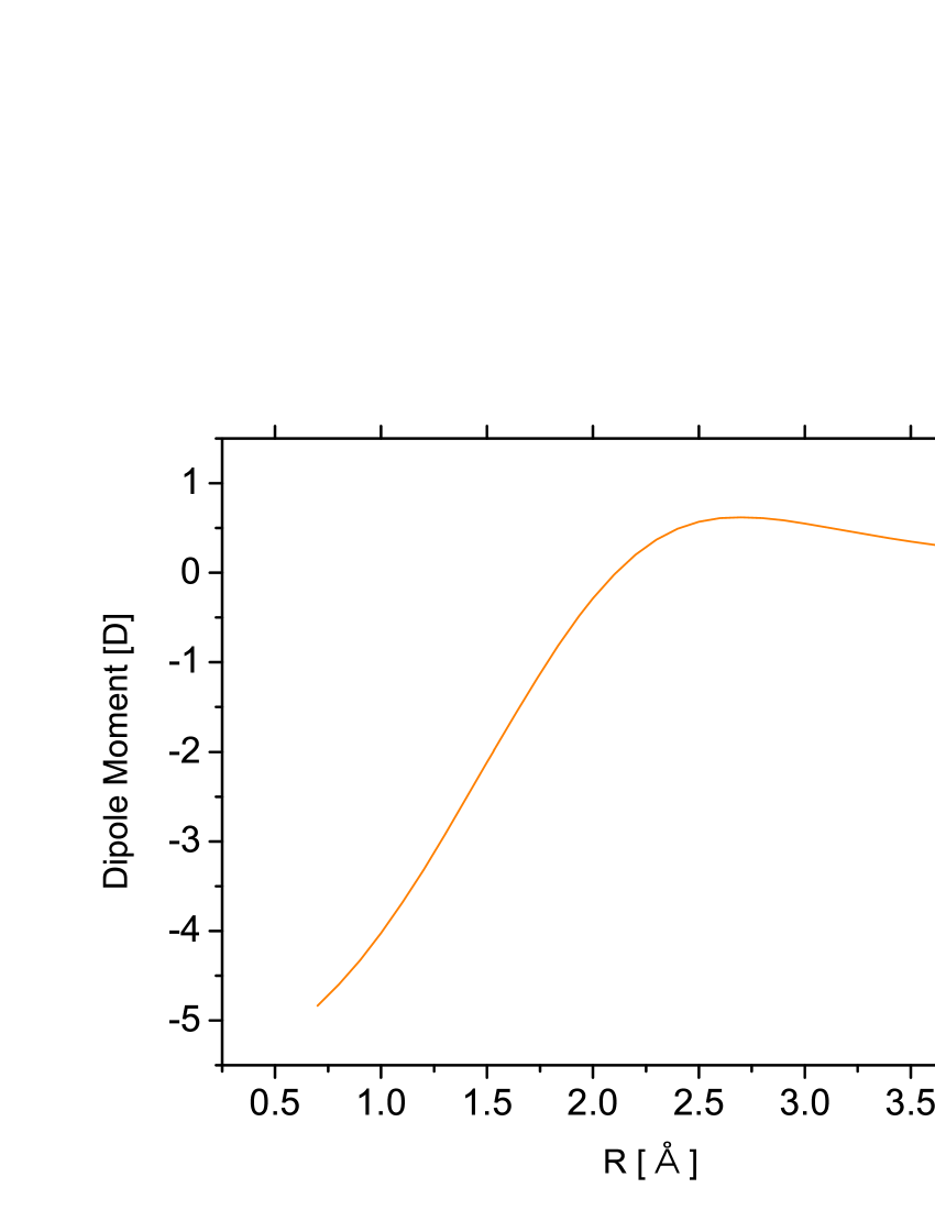
Figure 1: Dipole moment curve for CS obtained from the Padé expansion parameters of Pineiro et al. (1987).

2.3 Partition Functions

Partition function values for all 8 isotopologues of CS were calculated by a direct sum of all calculated energies for a range of temperatures. We determined that our partition function is at least 95% converged at 3000 K and much better than this at lower temperatures. Therefore temperatures up to 3000 K were considered. Partition function values for the parent isotopologue from CDMS and HITRAN (Laraia et al., 2011) are compared to the present work in Table 8.

At lower temperatures the CDMS partition function values are expected to be the most accurate and our values compare very well in this case. At higher temperatures only partition function values from HITRAN are available and our values are noticeably lower in this case. As the HITRAN partition function values are derived from using analytical approximations rather than a direct sum over energy levels, and do not agree as well with the CDMS values at lower temperatures, the results from this work are expected to be more accurate.

For ease of use, we fitted our partition functions, Q, to a series expansion of the form used by Vidler & Tennyson (2000):

$$\log_{10}Q(T)=\sum_{n=0}^{6}a_{n}\left[\log_{10}T\right]^{n}$$ (14)

with the $a_{n}$ values given in Table 9.

Table 8: Comparison of ¹²C³²S partition functions

T(K)	This work	CDMS	HITRAN
150	127.9828	127.9818	128.1770
300	256.3156	256.3136	257.0819
500	437.5903	437.5868	439.6790
1000	1018.57	-	1026.38
2000	2880.03	-	2910.73
3000	5705.80	-	5803.37

Table 9: Fitting parameters used to fit the partition functions. Fits are valid for temperatures between 500 and 3000 K.

	12C32S	12C33S	12C34S	12C36S	13C32S	13C33S	13C34S	13C36S
$a_{0}$	-80.005915	-76.155662	-80.005983	-80.004802	-79.895945	-79.450814	-79.753470	-72.151123
$a_{1}$	135.900176	130.515908	135.900484	135.901969	136.196073	136.926482	136.119795	132.718091
$a_{2}$	-92.069670	-88.464147	-92.068939	-92.067292	-92.226365	-92.982691	-92.125142	-99.251755
$a_{3}$	32.390529	31.162671	32.390765	32.392690	32.426480	32.752272	32.286797	39.931597
$a_{4}$	-6.167993	-5.950792	-6.168046	-6.170901	-6.170418	-6.233068	-6.095478	-9.136353
$a_{5}$	0.599177	0.581747	0.599173	0.600214	0.599063	0.603143	0.582017	1.139224
$a_{6}$	-0.022766	-0.022418	-0.022766	-0.022885	-0.022771	-0.022683	-0.021361	-0.060799

2.4 Line-List Calculations

Line lists were calculated for all stable isotopologues of CS (¹²C³²S, ¹²C³³S, ¹²C³⁴S, ¹²C³⁶S, ¹³C³²S, ¹³C³³S, ¹³C³⁴S and ¹³C³⁶S). These line lists span frequencies of up to 50,000 cm^-1. A summary of each line list is given in Table 10. All rotation-vibration states up to $v$ = 49 and $J$ = 258, and all transitions between these states satisfying the dipole selection rule $\Delta J=\pm 1$, were considered.

Table 10: Summary of our line lists.

	12C32S	12C33S	12C34S	12C36S	13C32S	13C33S	13C34S	13C36S
Maximum $v$	49	49	49	49	49	49	49	49
Maximum $J$	258	258	258	258	258	258	258	258
Number of lines	548312	550244	554898	560733	577885	581375	584485	590320

3 Results

The line lists contain over half a million transitions each. For compactness and ease of use they are separated into energy state and transitions files using the standard ExoMol format (Tennyson et al., 2013), which is based on a method originally developed for the BT2 line list (Barber et al., 2006). Extracts from the start of the ¹²C³²S files are given in Tables 11 and 12. The full line lists for all isotopologues considered can be downloaded from CDS, via ftp://cdsarc.u-strasbg.fr/pub/cats/J/MNRAS/xxx/yy, or http://cdsarc.u-strasbg.fr/viz-bin/qcat?J/MNRAS//xxx/yy or can be obtained from www.exomol.com.

Table 11: Extract from start of states file for ¹²C³²S. The full file can be downloaded from http://cdsarc.u-strasbg.fr/viz-bin/qcat?J/MNRAS//xxx/yy or www.exomol.com.

$n$	$\tilde{E}$	$g$	$J$	$v$
1	0.000000	1	0	0
2	1.634164	3	1	0
3	4.902459	5	2	0
4	9.804822	7	3	0
5	16.341155	9	4	0
6	24.511332	11	5	0

$n$: State counting number;
$\tilde{E}$: State energy in cm^-1;
$g$: State degeneracy;
$J$: State rotational quantum number;
$v$: State vibrational quantum number.

Table 12: Extracts from the transitions file for¹²C³²S. The full file can be downloaded from http://cdsarc.u-strasbg.fr/viz-bin/qcat?J/MNRAS//xxx/yy or www.exomol.com.

$F$	$I$	$A_{FI}$
2	1	1.7471E-06
3	2	1.6771E-05
4	3	6.0640E-05
5	4	1.4904E-04
6	5	2.9766E-04
7	6	5.2215E-04

$F$: Upper state counting number;
$I$: Lower state counting number;
$A_{FI}$: Einstein A coefficient in s^-1.

Table 13 compares our CS line lists with the previous ones from Pineiro et al. (1987) and CDMS; note that the 2078 CS transitions given in HITRAN-2012 (Rothman et al., 2013) are reproduced from CDMS. Although this is an assessment of the quantity of the data, not its quality, it demonstrates the reason for computing the new line lists, to provide a more comprehensive coverage of the problem.

Figure 2 provides an overview of CS absorption at infrared wavelengths as function of temperature. At 300 K, and below, the spectrum is dominated by a series of vibrational bands starting with the fundamental band at about 8 $\mu$m. At higher temperatures the bands become very much broader and their peak absorption is reduced.

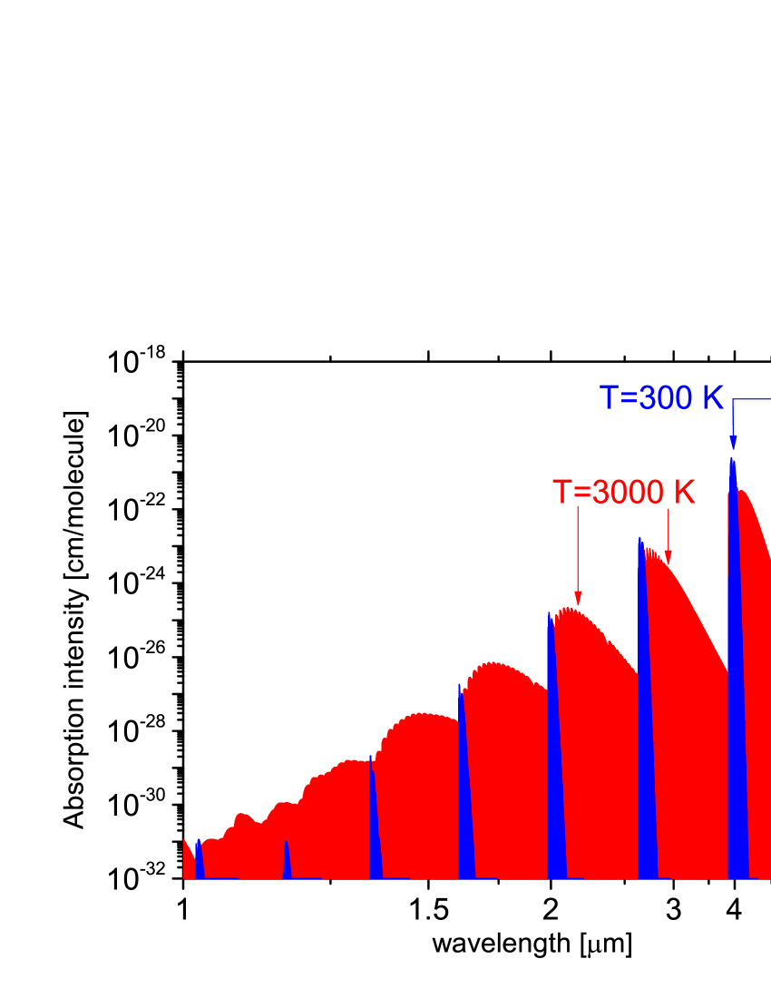
Figure 2: ¹²C³²S absorption spectrum at infrared wavelengths as calculated in this work for a temperature of 300 K (narrow features) and 3000 K (broad features).

Table 13: Comparison of CS rotation-vibration line lists. Given are the number of isotopologues considered, the maximum values for vibrational ($v$) and rotational ($J$) states considered, the maximum change in vibrational state ($\Delta v$) and whether intensity information and a partition function are provided.

Reference	Pineiro et al. (1987)	CDMS	This work
Isotopes	4	6	6
maximum $v$	20	4	49
maximum $J$	200	99	258
maximum $\Delta v$	4	2	50
Intensities?	Yes	Yes	Yes
Partition Function?	No	Yes	Yes

Comparisons with the CDMS rotational, $v^{\prime}-v^{\prime\prime}$ = 1 – 0 and $v^{\prime}-v^{\prime\prime}$ = 2 – 0 lines for ¹²C³²S are presented in Figure 3. The agreement is excellent for both frequency and intensity.

Ram et al. (1995) give two figures showing their observed spectrum, a compressed view of the vibration-rotation bands (1000 - 1400 cm^-1) and a portion of the R-branch region (1290 - 1310 cm^-1). Emission cross-sections for ¹²C³²S were simulated using a Gaussian line shape profile with HWHM = 0.01 cm^-1 as described in Hill et al. (2013). The resulting synthetic emission spectra are compared to the experimental spectra in Figures 4 and  5. For the former we the band structure and intensity ratio in our calculated spectra is very similar to the experiment. For the latter there is generally good agreement; however the intensities of five strongest lines are almost 50 % larger in the theoretical spectrum which may be due to saturation effects in the measured spectrum.

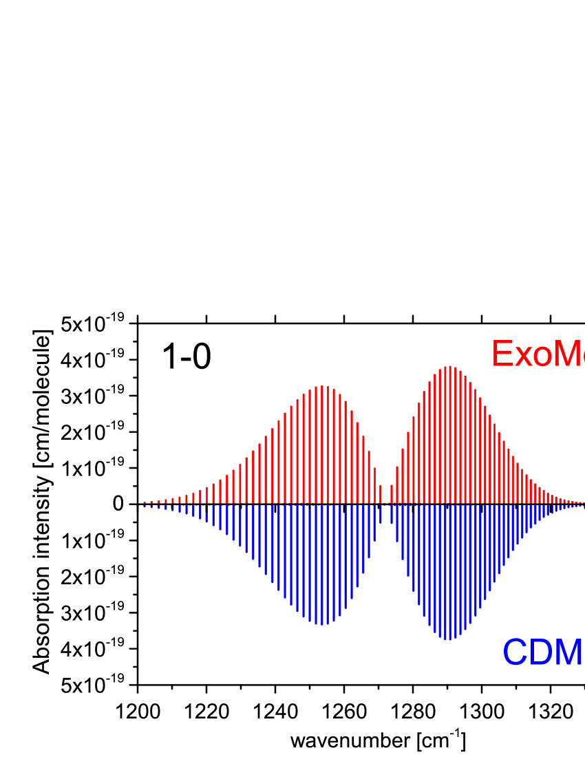
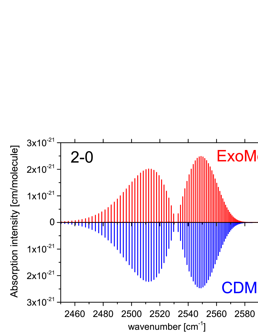
Figure 3: Absorption lines of ¹²C³²S at 300 K: ExoMol verses CDMS

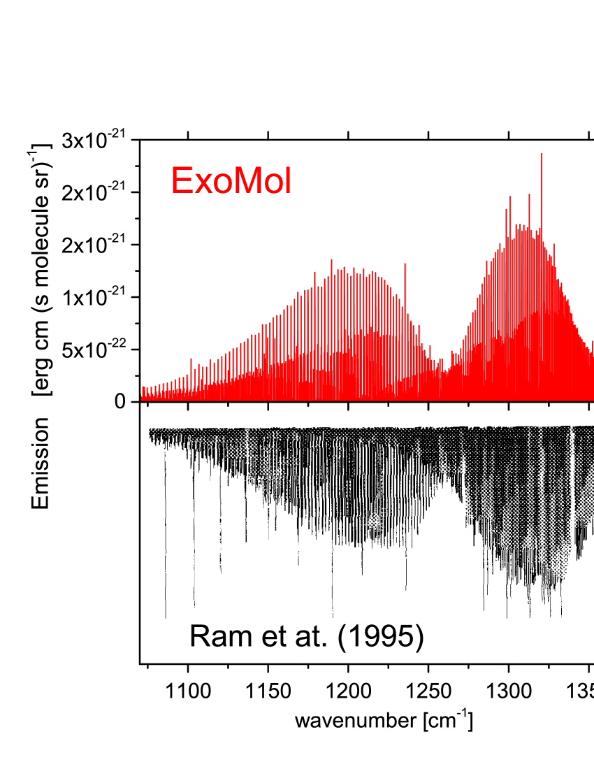
Figure 4: ¹²C³²S at 2300 C: Emission spectrum upper, Ram et al. (1995); Emission lines lower, ExoMol. [Reprinted from Ram et al. (1995)]

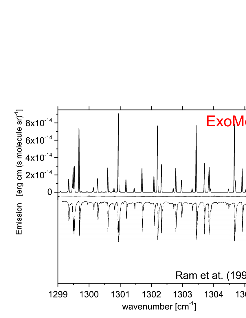
Figure 5: Emission spectrum of ¹²C³²S at 2300 C: upper, Ram et al. (1995); lower, ExoMol. [Reprinted from Ram et al. (1995)]

4 Conclusions

In the present work we have computed comprehensive line lists for all stable isotopologues of carbon monosulphide. We determined a PEC using LEVEL and modified potential parameters from the literature. We then substituted calculated energies in the states file with energies derived directly from experimental frequencies to match the experimental accuracy. This accuracy should extend to all predicted transition frequencies up to at least $v$ = 9 and $J$ = 106 for ¹²C³²S, and $v$ = 5 and $J$ = 80 for ¹³C³²S, the experimental ranges. Based on comparisons with other experiments the frequencies for the remaining isotopologues should be predicted to sub-wavenumber accuracy at least for v < 3 and J < 21. Einstein A coefficients were computed from a dipole moment curve taken from the literature. Comparisons with the semi-empirical CDMS database suggest that the pure rotational, $v^{\prime}-v^{\prime\prime}$ = 1 – 0, and $v^{\prime}-v^{\prime\prime}$ = 2 – 0 intensities are accurate.

The results are line lists for rotation-vibration transitions within the ground states of ¹²C³²S, ¹²C³³S, ¹²C³⁴S, ¹²C³⁶S, ¹³C³²S, ¹³C³³S, ¹³C³⁴S and ¹³C³⁶S, which should be accurate for a range of temperatures up to at least 3000 K. The line lists can be downloaded from CDS or from www.exomol.com.

Finally we note that, although our line lists are more comprehensive, for the purposes of high resolution radio astronomy and far-infrared studies of the low temperature objects, the CDMS line lists are recommended.

References

- Agundez & Cernicharo (2006) Agundez M., Cernicharo J., 2006, ApJ, 650, 374
- Ahrens & Winnewisser (1999) Ahrens V., Winnewisser G., 1999, Z. Naturforsch, 54a, 131
- Barber et al. (2014) Barber R. J., Strange J. K., Hill C., Polyansky O. L., Mellau G. C., Yurchenko S. N., Tennyson J., 2014, MNRAS, 437, 1828
- Barber et al. (2006) Barber R. J., Tennyson J., Harris G. J., Tolchenov R. N., 2006, MNRAS, 368, 1087
- Barton et al. (2014) Barton E. J., Chiu C., Golpayegani S., Yurchenko S. N., Tennyson J., Frohman D. J., Bernath P. F., 2014, MNRAS, 442, 1821
- Barton et al. (2013) Barton E. J., Yurchenko S. N., Tennyson J., 2013, MNRAS, 434, 1469
- Bell et al. (1972) Bell S., Ng T., Suggitt C., 1972, J. Mol. Spectrosc., 44, 267
- Bilalbegovic & Baranovic (2015) Bilalbegovic G., Baranovic G., 2015, MNRAS, 446, 3118
- Bogey et al. (1981) Bogey M., Demuynck C., Destombes J., 1981, Chem. Phys. Lett., 81, 256
- Bogey et al. (1982) Bogey M., Demuynck C., Destombes J., 1982, J. Mol. Spectrosc., 95, 35
- Botschwina & Sebald (1985) Botschwina P., Sebald P., 1985, J. Mol. Spectrosc., 110, 1
- Bregman et al. (1978) Bregman J. D., Goebel J. H., Strecker D., 1978, ApJ, 223, L45
- Burkholder et al. (1987) Burkholder J. B., Lovejoy E., Hammer P. D., Howard C. J., 1987, J. Mol. Spectrosc., 124, 450
- Canaves et al. (2007) Canaves M., de Almeida A., Boice D., Sanzovo G., 2007, Adv. Space Res., 39, 451
- Cossart et al. (1977) Cossart D., Horani M., Rostas J., 1977, J. Mol. Spectrosc., 67, 283
- Coxon & Colin (1997) Coxon J. A., Colin R., 1997, J. Mol. Spectrosc., 181, 215
- Coxon & Hajigeorgiou (1992) Coxon J. A., Hajigeorgiou P. G., 1992, Chem. Phys., 167, 327
- Crawford & Shurcliff (1934) Crawford F. H., Shurcliff W. A., 1934, Phys. Rev., 45, 860
- Davis et al. (2013) Davis T., Bayet E., Crocker A., Topal S., Bureau M., 2013, MNRAS, 433, 1659
- Furtenbacher et al. (2007) Furtenbacher T., Császár A. G., Tennyson J., 2007, J. Mol. Spectrosc., 245, 115
- Gottlieb et al. (2003) Gottlieb C. A., Myers P. C., Thaddeus P., 2003, ApJ, 588, 655
- Hajigeorgiou & Le Roy (2000) Hajigeorgiou P. G., Le Roy R. J., 2000, J. Chem. Phys., 112, 3949
- Henkel & Bally (1985) Henkel C., Bally J., 1985, A&A, 150, L25
- Henkel et al. (1993) Henkel C., Mauersberger R., Wiklind T., Huettemeister S., Lemme C., Millar T. J., 1993, A&A, 268, L17
- Hill et al. (2013) Hill C., Yurchenko S. N., Tennyson J., 2013, Icarus, 226, 1673
- Kewley et al. (1963) Kewley R., Sastry K., Winnewisser M., Gordy W., 1963, J. Chem. Phys., 39, 2856
- Kim & Yamamoto (2003) Kim E., Yamamoto S., 2003, J. Mol. Spectrosc., 219, 296
- Laraia et al. (2011) Laraia A. L., Gamache R. R., Lamouroux J., Gordon I. E., Rothman L. S., 2011, Icarus, 215, 391
- Le Roy (2007) Le Roy R. J., 2007, LEVEL 8.0 A Computer Program for Solving the Radial Schrödinger Equation for Bound and Quasibound Levels. University of Waterloo Chemical Physics Research Report CP-663, http://leroy.uwaterloo.ca/programs/
- Li et al. (2013) Li C., Deng L., Zhang J., Qiu X., Wei J., Chen Y., 2013, J. Mol. Spectrosc., 284, 29
- Lovas & Krupenie (1974) Lovas F., Krupenie P., 1974, J. Phys. Chem. Ref. Data, 3, 245
- Mauersberger et al. (1989a) Mauersberger R., Henkel C., Wilson T., Harju J., 1989a, A&A, 226, L5
- Mauersberger et al. (1989b) Mauersberger R., Henkel C., Wilson T., Harju J., 1989b, A&A, 223, 79
- McQuinn et al. (2002) McQuinn K. B. W., Simon R., Law C. J., Jackson J. M., Bania T. M., Clemens D. P., Heyer M. H., 2002, ApJ, 576, 274
- Mockler & Bird (1955) Mockler R. C., Bird G. R., 1955, Phys. Rev., 98, 1837
- Moreno et al. (2003) Moreno R., Marten A., Matthews H. E., Biraud Y., 2003, PlanetSpaceSci, 51, 591
- Müller et al. (2005) Müller H. S. P., Schlöder F., Stutzki J., Winnewisser G., 2005, J. Molec. Struct. (THEOCHEM), 742, 215
- Nilsson et al. (2000) Nilsson A., Bergman P., Hjalmarson A., 2000, ApJS, 144, 441
- Orton et al. (1995) Orton G. et al., 1995, Science, 267, 1277
- Patrascu et al. (2015) Patrascu A. T., Tennyson J., Yurchenko S. N., 2015, MNRAS, 449, 3613
- Penzias et al. (1971) Penzias A. A., Solomon P. M., Wilson R. W., Jefferts K. B., 1971, ApJ, 168, L53
- Pineiro et al. (1987) Pineiro A. L., Tipping R. H., Chackerian Jr C., 1987, J. Mol. Spectrosc., 125, 91
- Ram et al. (1995) Ram R. S., Bernath P. F., Davis S. P., 1995, J. Mol. Spectrosc., 173, 146
- Rivlin et al. (2015) Rivlin T., Lodi L., Yurchenko S. N., Tennyson J., Le Roy R. J., 2015, MNRAS, 451, 5153
- Rothman et al. (2013) Rothman L. S. et al., 2013, J. Quant. Spectrosc. Radiat. Transf., 130, 4
- Scoville et al. (2015) Scoville N. et al., 2015, ApJ, 800, 70
- Shi et al. (2011) Shi D., Li W., Zhang X., Sun J., Liu Y., Zhu Z., Wang J., 2011, J. Mol. Spectrosc., 266, 27
- Stark et al. (1987) Stark G., Yoshino K., Smith P. L., 1987, J. Mol. Spectrosc., 124, 420
- Tennyson et al. (2013) Tennyson J., Hill C., Yurchenko S. N., 2013, in AIP Conference Proceedings, Vol. 1545, 6th international conference on atomic and molecular data and their applications ICAMDATA-2012, AIP, New York, pp. 186–195
- Tennyson & Yurchenko (2012) Tennyson J., Yurchenko S. N., 2012, MNRAS, 425, 21
- Todd (1977) Todd T. R., 1977, J. Mol. Spectrosc., 66, 162
- Todd & Olson (1979) Todd T. R., Olson W. B., 1979, J. Mol. Spectrosc., 74, 190
- Uehara et al. (2015) Uehara H., Horiai K., Sakamoto Y., 2015, J. Mol. Spectrosc., 313, 19
- Vidler & Tennyson (2000) Vidler M., Tennyson J., 2000, J. Chem. Phys., 113, 9766
- Winkel et al. (1984) Winkel R. J., Davis S. P., Pecyner R., Brault J. W., 1984, Can. J. Phys., 62, 1414
- Winnewisser & Cook (1968) Winnewisser G., Cook R. L., 1968, J. Mol. Spectrosc., 28, 266
- Yadin et al. (2012) Yadin B., Vaness T., Conti P., Hill C., Yurchenko S. N., Tennyson J., 2012, MNRAS, 425, 34
- Yamada & Hirota (1979) Yamada C., Hirota E., 1979, J. Mol. Spectrosc., 74, 203
- Yorke et al. (2014) Yorke L., Yurchenko S. N., Lodi L., Tennyson J., 2014, MNRAS, 445, 1383