The classical mutual information in mean-field spin glass models

Abstract

We investigate the classical Rényi entropy $S_{n}$ and the associated mutual information ${\mathcal{I}}_{n}$ in the Sherrington-Kirkpatrick (S-K) model, which is the paradigm model of mean-field spin glasses. Using classical Monte Carlo simulations and analytical tools we investigate the S-K model on the $n$-sheets booklet. This is obtained by gluing together $n$ independent copies of the model, and it is the main ingredient to construct the Rényi entanglement-related quantities. We find a glassy phase at low temperature, whereas at high temperature the model exhibits paramagnetic behavior, consistent with the regular S-K model. The temperature of the paramagnetic-glassy transition depends non-trivially on the geometry of the booklet. At high-temperatures we provide the exact solution of the model by exploiting the replica symmetry. This is the permutation symmetry among the fictitious replicas that are used to perform disorder averages (via the replica trick). In the glassy phase the replica symmetry has to be broken. Using a generalization of the Parisi solution, we provide analytical results for $S_{n}$ and ${\mathcal{I}}_{n}$, and for standard thermodynamic quantities. Both $S_{n}$ and ${\mathcal{I}}_{n}$ exhibit a volume law in the whole phase diagram. We characterize the behavior of the corresponding densities $S_{n}/N,{\mathcal{I}}_{n}/N$, in the thermodynamic limit. Interestingly, at the critical point the mutual information does not exhibit any crossing for different system sizes, in contrast with local spin models.

I Introduction

Besides being ubiquitous in nature, disorder leads to several intriguing physical phenomena. Arguably, spin glasses represent one of the most prototypical examples of interesting behavior induced by disorder. While at any finite temperature disorder can prevent the usual magnetic ordering, at low-enough temperatures these systems display a new type of “order”. In the past decades an intense theoretical effort has been devoted to characterizing this spin glass order, the nature of the paramagnetic-glassy transition, and that of the associated order parameter binder-1986 ; parisi-book ; young-1998 ; nishimori-book ; castellani-2005 .

All these issues can be thoroughly addressed in the Sherrington-Kirkpatrick (S-K) model sherrington-1978 ; sherrington-1978-prl , which is exactly solvable. The S-K model is a classical Ising model on the fully-connected graph of $N$ sites, with quenched random interactions. Its hamiltonian reads

$${\mathcal{H}}=-\sum\limits_{1\leq i<j\leq N}J_{ij}S_{i}S_{j}-h\sum\limits_{1\leq i\leq N}S_{i}.$$ (1)

Here $S_{i}=\pm 1$ are classical Ising spins, $h$ is an external magnetic field, and $J_{ij}$ are uncorrelated (from site to site) random variables. The S-K model hosts a low-temperature glassy phase, which is separated from a high-temperature paramagnetic one by a second order phase transition. Despite its mean-field nature, the solution of the S-K model has been a mathematical challenge. Although it was proposed as an ansatz by Parisi parisi-1980 more than thirty years ago, its rigorous proof was obtained only recently talagrand-2006 . Moreover, the solution exhibits several intricate features, such as lack of self-averaging pastur-1991 , ultrametricity mezard-1984 ; rammal-1986 , and replica symmetry breaking parisi-book ; castellani-2005 . The last refers to the breaking of the permutation symmetry among the fictitious replicas of the model, which are introduced to perform disorder averages (via the so-called replica trick cardy-book . Finally, although the applicability of the S-K model to describe realistic spin glasses is still highly debated yucesoy-2012 ; billoire-2012 ; yucesoy-2013 , there are recent proposals on how to realize it in cold-atomic gases morrison-2008 ; rotondo-2015 , or in laser systems ghofraniha-2015 .

In the last decade entanglement-related quantities emerged as valuable tools to understand the physics of complex systems amico-2008 ; eisert-2009 ; calabrese-2009 ; cc-rev , both classical and quantum. For instance, at a conformally invariant critical point entanglement measures contain universal information about the underlying conformal field theory (CFT), such as the central charge holzhey-1994 ; vidal-2003 ; calabrese-2004 ; calabrese-2012 . For classical spin models a lot of attention has been focused on the classical Rényi entropy jaconis-2013 ; stephan-2014 . Given a bipartition of the system into two complementary subregions $A$ and $B$, the classical Rényi entropy $S_{n}(A)$ (with $n\in\mathbb{N}$) is defined as

$$S_{n}(A)\equiv\frac{1}{1-n}\log\Big{(}\sum\limits_{i_{A}\in{\mathcal{C}}_{A}}p^{n}_{i_{A}}\Big{)}$$ (2)

Here ${\mathcal{C}}_{A}$ denotes the set of all the possible spin configurations in part $A$, whereas $p_{i_{A}}$ is the probability of the configuration $i_{A}$. Alternatively, $S_{n}(A)$ can be obtained from the partition function of the model on an ad hoc defined “booklet” geometry (see section II for its definition). This consists of $n$ independent and identical copies (the booklet “sheets”) of the model. These physical copies are different from the fictitious replicas used to perform the disorder average. Each sheet is divided into two parts $A$ and $B$, containing $N_{A}$ and $N_{B}$ spins, respectively. The spins in part $A$ of different sheets are constrained to be equal. It is convenient to introduce the booklet aspect ratio $0\leq\omega\leq 1$ as

$$\omega\equiv\frac{N_{A}}{N}.$$ (3)

For local spin models the bipartition correspond to a spatial separation between the spins. However, the definition (2) can be used in models with no notion of space, where it quantifies the correlation between two groups of spins rathen than two spatial regions. Notice that Eq. (2) can also be used for quantum systems by replacing the sum over the proababilities of each state in region $A$ with the trace over the reduced density matrix for region $A$. For $n=1$ Eq. (2) defines the subsystem Shannon entropy alcaraz-2013 ; stephan-2014-a . From $S_{n}(A)$, one defines the classical mutual information ${\mathcal{I}}_{n}(A,B)$ as

$${\mathcal{I}}_{n}(A,B)\equiv S_{n}(A)+S_{n}(B)-S_{n}(A\cup B).$$ (4)

For local models ${\mathcal{I}}_{n}$ obeys the area law wolf-2008 ${\mathcal{I}}_{n}(A)\propto\ell$, with $\ell$ the length of the boundary between $A$ and $B$. Remarkably, for different $\ell$, the ratio ${\mathcal{I}}_{n}/\ell$ has been shown to exhibit a crossing at a second order phase transition jaconis-2013 , implying that it can be used as a diagnostic tool for critical behaviors. For conformally invariant critical models more universal information can be extracted from the area-law corrections of ${\mathcal{I}}_{n}$ stephan-2014 .

Although recently the study of the interplay between disorder and entanglement became a fruitful research area refael-2009 , the behavior of entanglement-related quantities in glassy phases, and at glassy critical points, has not been explored yet (see, however, Ref. castelnovo-2010, for some interesting results). Here we investigate both the classical Rényi entropy $S_{n}(A)$ and the mutual information ${\mathcal{I}}_{n}$ in the S-K model, using classical Monte Carlo simulations and analytical tools. We often restrict ourselves to the case with $n=2$, as this is where numerical simulations are most efficient. As usual in disordered system, we focus on disorder-averaged quantities, considering $[S_{n}]$ and $[{\mathcal{I}}_{n}]$, with the brackets $[\cdot]$ denoting the average over different realizations of $J_{ij}$ (cf. Eq. (1)).

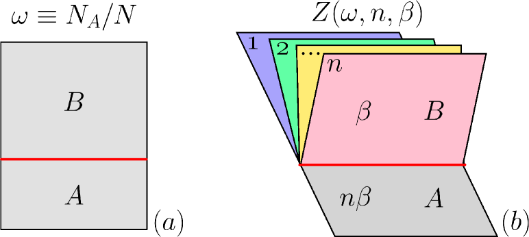
Figure 1: The booklet geometry considered in this work. (a) The single sheet (“page”) of the booklet: The $N$ spins living on the sheet are divided into two groups $A$ and $B$, containing $N_{A}$ and $N_{B}$ spins, respectively. Here $\omega\equiv N_{A}/N$ is the booklet ratio. (b) The $n$ sheets are glued together to form the booklet. The spins in part $B$ of the booklet pages are at inverse temperature $\beta$. The spins in part $A$ are identified (see Eq. (8)). As a consequence, the effective temperature in part $A$ is $n\beta$. $Z(\omega,n,\beta)$ denotes the partition function of the S-K model on the booklet.

The Article is organized as follows. In section II we introduce the classical Rényi entropy and the mutual information, reviewing their representation in terms of the booklet partition functions. In section III we present the structure of the solution of the S-K model on the booklet. Specifically, we discuss the replica trick, which is used to perform disorder averages, and the saddle point approximation in the thermodynamic limit. Section IV is concerned with the RS approximation. In subsection IV.1 we focus on the high-temperature region, where this approximation becomes exact. In subsection IV.3 we discuss the structure of the RS ansatz in the low-temperature region. Section V is devoted to the $1$-RSB approximation. In section VI we check the validity of both the RS and the $1$-RSB results comparing with Monte Carlo simulations for the internal energy. Section VII and section VIII discuss the classical Rényi entropy and the mutual information, respectively. We conclude in section IX.

II The booklet construction & and the classical Rényi entropy

Given a generic classical spin model at inverse temperature $\beta$, The probability $p_{i}$ of a given spin configuration $i\in{\mathcal{C}}$, with ${\mathcal{C}}$ being the set of all possible configurations, is given by the Boltzmann weight $p_{i}=e^{-\beta E(i)}/Z$, with $E(i)$ the associated energy. In presence of a bipartition (see Fig. 1 (a)) the probability of a spin configuration $i_{A}\in{\mathcal{C}}_{A}$ is given as $p_{i_{A}}=\sum_{i_{B}}e^{-\beta E(i_{A},i_{B})}/Z$, where the sum is over all possible spin configurations in part $B$. Note that this is valid for generic interactions, i.e., both local and non-local ones. Clearly, one has $p^{n}_{i_{A}}\equiv\frac{1}{Z^{n}}\sum_{(i^{1}_{B},\dots,i^{n}_{B})}e^{-\beta\sum_{k}E(i_{A},i^{k}_{B})}$. Thus, the classical Rényi entropy $S_{n}(A)$ (Eq. (2)) can be calculated as jaconis-2013 ; stephan-2014

$$S_{n}(A)\equiv\frac{1}{1-n}\log\left(\frac{Z(A,n,\beta)}{Z^{n}(\beta)}\right).$$ (5)

Here $Z(A,n,\beta)\equiv\sum_{i_{A},(i_{B}^{1},\dots,i_{B}^{n})}e^{-\beta\sum_{k}E(i_{A},i^{k}_{B})}$ can be interpreted as the partition function of the model on the $n$-sheet booklet (with $k$ labelling its different sheets), whereas $Z(\beta)$ is the partition functions on the plane at inverse temperatures $\beta$. The booklet geometry is illustrated in Fig. 1, and consists of $n$ identical copies (“sheets”) of the system. Each sheet is divided into two parts $A$ and $B$ (cf. Fig. 1 (a)). The spins in part $A$ of the different sheets are identified (cf. Fig. 1 (b)). While spins in parts $B$ of the booklet are at inverse temperature $\beta$, the ones in $A$ are at the effective temperature $n\beta$. Notice that a similar geometric construction guerra-2002 plays an important role in the mathematical proof of the Parisi ansatz. Moreover, the study of the partition function of critical models on the booklet has attracted considerable attention recently fradkin-2006 ; fradkin-2009 ; hsu-2009 ; stephan-2009 ; hsu-2010 ; oshikawa-2010 ; stephan-2010 ; zaletel-2011 . Clearly, one has $S_{n}(A)\equiv 1/(n-1)(\log(F(A,n,\beta))-n\log(F(\beta)))$, where $F(A,n,\beta)\equiv\log(Z(A,n\beta))$ and $F(\beta)\equiv\log(Z(\beta))$ are related (apart from a factor $-1/\beta$) to the free energy of the model on the booklet and on the plane, respectively.

The mutual information ${\mathcal{I}}_{n}(A,B,\beta)$ is obtained in terms of the booklet partition functions using Eq. (5) and Eq. (4), where $S_{n}(B)$ is obtained from (5) by exchanging $A$ and $B$. Notice also that in (5) $Z(A\cup B,n,\beta)\equiv Z(n\beta)$ is the partition function of the model on the booklet with all the $n$ sheets identified, equivalently on a single sheet but at temperature $n\beta$. Notice that the disorder-averaged mutual information $[{\mathcal{I}}_{n}]$ and the Rényi entropy $[S_{n}]$ are directly related to the so-called quenched-averaged free energy $[F(A,n,\beta)]$, which is the main quantity of interest in disordered systems cardy-book . For clean (i.e., without disorder) local spin models ${\mathcal{I}}_{n}$ obeys the boundary law

$${\mathcal{I}}_{n}(A,B,\beta)=\alpha_{n}\ell+{\mathcal{G}}_{n}+\gamma_{n},$$ (6)

with $\ell$ the length of the boundary between $A$ and $B$, and $\alpha_{n},\gamma_{n}$ two non-universal constants. Here ${\mathcal{G}}_{n}$ is the so-called geometric mutual information stephan-2014 . Interestingly, for critical systems ${\mathcal{G}}_{n}$ depends only on the geometry of $A$ and $B$, and it is universal. For conformally invariant models ${\mathcal{G}}_{n}$ can be calculated using standard methods of conformal field theory (CFT), and it allows to numerically extract universal information about the CFT, such as the central charge stephan-2014 .

III The Sherrington-Kirkpatrick (S-K) model on the booklet

Here we introduce the Sherrington-Kirkpatrick (S-K) model on the booklet. In subsection III.1 we define the model and its partition function. In subsection III.2 we discuss the replicated booklet construction that is used to calculate the disorder-averaged free energy $[F(\omega,n,\beta)]$. In section III.3 we consider the thermodynamic limit, using the saddle point approximation. We also introduce the overlap tensor, which contains all the information about the thermodynamic behavior of the model. The analytical formula for the replicated partition function (Eq. (19)), and the saddle point equations (Eqs. (22)(23)) for the overlap tensor are the main results of this section.

III.1 The model and its partition function

The Sherrington-Kirkpatrick (S-K) model sherrington-1978-prl ; sherrington-1978 on the $n$-sheets booklet (cf. Fig. 1) is defined by the Hamiltonian

$${\mathcal{H}}=-\sum\limits_{r=1}^{n}\left\{\sum\limits_{i<j}J_{ij}S^{(r)}_{i}S^{(r)}_{j}-h\sum\limits_{i=1}^{N}S^{(r)}_{i}\right\}.$$ (7)

Here $S_{i}^{(r)}=\pm 1$ are classical Ising spins, $r\in[1,n]$ labels the different sheets (“pages”) of the booklet, $i\in[1,N]$ denotes the sites on each sheet, $J_{ij}$ is the interaction strength, and $h$ is an external magnetic field. The total number of spins in the booklet is $nN$. The first sum inside the brackets in Eq. (7) is over all the $N(N-1)/2$ pairs of spins in each sheet. Spins on different sheets do not interact. In each “sheet” all the sites are divided into two groups $A\equiv\{1,\dots,N_{A}\}$ and $B\equiv\{N_{A}+1,\dots,N\}$, containing $N_{A}$ and $N_{B}\equiv N-N_{A}$ sites, respectively. The spins living in part $A$ and different sheets are identified, i.e. one has

$$S_{i}^{(r)}=S_{i}^{(r^{\prime})}\quad\forall\,i\in A,r,r^{\prime}.$$ (8)

Since in each sheet all spins interact with each other, there is no notion of distance between different spins. Thus, physical observables should depend on the booklet geometry only through the ratio $\omega$ (cf. Eq. (3)).

In Eq. (7) the couplings $J_{ij}\in\mathbb{R}$ are uncorrelated (from site to site) quenched random variables. $J_{ij}$ are the same in all the sheets of the booklet. Specifically, here $J_{ij}$ are drawn from the gaussian distribution

$$P(J_{ij})=\left(\frac{N}{2\pi}\right)^{1/2}\exp\Big{\{}-\frac{N}{2J^{2}}\Big{(}J_{ij}-\frac{J_{0}}{N}\Big{)}^{2}\Big{\}}.$$ (9)

The mean and the variance of $P(\{J_{ij}\})$ are given as $[J_{ij}]=J_{0}/N$ and $[(J_{ij}-[J_{ij}])^{2}]=J^{2}/N$, respectively. Here we set $J=1$. The square brackets $[\cdot]$ denote the average over different realizations of $J_{ij}$. Here we restrict ourselves to $J_{0}=0$ and $J=1$. The factors $N$ in Eq. (9) ensure a well-defined thermodynamic limit.

The partition function $Z(\omega,n,\beta,\{J\})$ of the S-K model on the booklet at inverse temperature $\beta\equiv 1/T$, and for fixed disorder realization $\{J_{ij}\}$, reads

$$Z(\omega,n,\beta,\{J\})\equiv\textrm{Tr}^{\prime}\exp(-\beta{\mathcal{H}})=\\ \textrm{Tr}^{\prime}\exp\Big{\{}\beta\sum\limits_{r}\Big{(}\sum\limits_{i<j}J_{ij}S^{(r)}_{i}S^{(r)}_{j}-h\sum\limits_{i=1}^{N}S^{(r)}_{i}\Big{)}\Big{\}},$$ (10)

where $\textrm{Tr}^{\prime}\equiv\sum_{\{S_{i}\}}$ denotes the sum over all possible spin configurations. The prime in $\textrm{Tr}^{\prime}$ stresses that only spin configurations satisfying the constraint in Eq. (8) are considered. In the two limits $\omega=0$ and $\omega=1$ one recovers the standard S-K model. In particular, for $\omega=0$, i.e., $n$ disconnected sheets, one has $Z(0,n,\beta,\{J\})=Z(\beta,\{J\})^{n}$, with $Z(\beta,\{J\})$ the partition function of the S-K model on the plane (i.e., the original S-K model). On the other hand, for $\omega=1$ it is $Z(1,n,\beta,\{J\})=Z(n\beta,\{J\})$, i.e., the partition function of the S-K model at inverse temperature $n\beta$. The quenched averaged free energy $[F(\omega,n,\beta)]$, is defined as

$$[F(\omega,n,\beta)]\equiv-\frac{1}{\beta}\int{\mathcal{D}}\{J\}\log Z(\omega,n,\beta,\{J\}),$$ (11)

where $\int{\mathcal{D}}\{J\}\equiv\prod\nolimits_{i<j}\int_{-\infty}^{+\infty}dJ_{ij}P(J_{ij})$.

At $\omega=0$ and $\omega=1$ the phase diagram of the S-K model in the thermodynamic limit is well established parisi-book ; nishimori-book . At $\omega=0$ it exhibits a standard paramagnetic phase in the high temperature region, whereas at low temperatures a glassy phase is present, with replica-symmetry breaking. The two phases are divided by a second order phase transition at $\beta=\beta_{c}=1$. The phase diagram for $\omega=1$ is the same, apart from the trivial rescaling $\beta\to n\beta$. We anticipate here (see section IV.3) that a similar scenario holds for generic $\omega$. Specifically, the glassy replica-symmetry-broken phase at low temperatures survives for generic $0<\omega<1$, while at high enough temperature the model is paramagnetic. The critical point, which marks the transition between the two phases, is a nontrivial function of the booklet ratio $\omega$ (see section IV.4).

III.2 The replicated booklet and the overlap tensor

The disorder-averaged free energy $[F(\omega,n,\beta)]$ (cf. Eq. (11)) of the model is obtained, using the standard replica trick cardy-book , as

$$[F(\omega,n,\beta)]=\lim_{\alpha\to 0}\frac{[Z^{\alpha}(\omega,n,\beta)]-1}{\alpha}.$$ (12)

Here $[Z^{\alpha}(\omega,n,\beta)]$ is the disorder-averaged partition function of $\alpha\in\mathbb{N}$ independent copies of the S-K model on the booklet. Precisely, $[Z^{\alpha}(\omega,n,\beta)]$ reads

$$[Z^{\alpha}(\omega,n,\beta)]=\int{\mathcal{D}}\{J\}\textrm{Tr}^{\prime}\exp\sum\limits_{r,\gamma}\Big{\{}\\ \beta\sum\limits_{i<j}J_{ij}S_{i}^{(r,\gamma)}S_{j}^{(r,\gamma)}+\beta h\sum\limits_{i}S^{(r,\gamma)}_{i}\Big{\}},$$ (13)

where the index $\gamma=1,2,\dots,\alpha$ labels the different fictitious replicas introduced in Eq. (12), whereas $r$ denote the physical copies, i.e., the booklet sheets, as in Eq. (10). Again, spins on different sheets or different replicas do not interact with each other. Notice that $Z^{\alpha}(\omega,n,\beta)$ can be thought of as the partition function of the S-K model on a “replicated” booklet.

Using Eq. (9), the disorder average in Eq. (13) can be performed explicitly, to obtain

$$[Z^{\alpha}(\omega,n,\beta)]=\textrm{Tr}^{\prime}\exp\sum\limits_{r,\gamma}\Big{\{}\\ \frac{1}{N}\sum\limits_{i<j}\Big{(}\frac{\beta^{2}}{2}\sum\limits_{\gamma^{\prime},r^{\prime}}S^{(r,\gamma)}_{i}S^{(r,\gamma)}_{j}S^{(r^{\prime},\gamma^{\prime})}_{i}S^{(r^{\prime},\gamma^{\prime})}_{j}\\ +\beta J_{0}S_{i}^{(r,\gamma)}S_{j}^{(r,\gamma)}\Big{)}+\beta h\sum\limits_{i}S_{i}^{(r,\gamma)}\Big{\}}.$$ (14)

In contrast with Eq. (13), both different sheets and different replicas are now coupled by a four-spin interaction. It is convenient to introduce the Hubbard-Stratonovich variables $q_{\gamma\gamma^{\prime}}^{rr^{\prime}}$ and $m_{\gamma}^{r}$. Following the spin glass literature parisi-book , we dub $q_{\gamma\gamma^{\prime}}^{rr^{\prime}}$ the overlap tensor. In the standard S-K model (i.e., for $n=1$) $q_{\gamma\gamma^{\prime}}^{rr^{\prime}}$ becomes a $\alpha\times\alpha$ matrix sherrington-1978-prl . Eq. (14) now yields

$$[Z^{\alpha}(\omega,n,\beta)]=\exp\Big{(}\frac{\beta^{2}Nn\alpha}{4}\Big{)}\int\prod_{\begin{subarray}{c}\gamma\leq\gamma^{\prime}\\ r,r^{\prime}\end{subarray}}dq^{rr^{\prime}}_{\gamma\gamma^{\prime}}\int\prod_{\gamma,r}dm_{\gamma}^{r}\\ \textrm{Tr}^{\prime}\exp\Big{\{}-N{\mathcal{K}}(\{q,m\})+\sum_{i}{\mathcal{L}}_{i}(\{q,m\})\Big{\}},$$ (15)

where we neglected subleading contributions ${\mathcal{O}}(1/N)$ in the thermodynamic limit. Here ${\mathcal{K}}(\{q,m\})$ is spin-independent and it reads

$${\mathcal{K}}(\{q,m\})\equiv\frac{\beta^{2}}{2J_{0}}\Big{(}\sum\limits_{\gamma<\gamma^{\prime}}\sum\limits_{r,r^{\prime}}(q_{\gamma\gamma^{\prime}}^{rr^{\prime}})^{2}\\ +\sum\limits_{\gamma}\sum\limits_{r<r^{\prime}}(q_{\gamma\gamma}^{rr^{\prime}})^{2}\Big{)}+\frac{\beta}{2J_{0}}\sum\limits_{\gamma r}(m_{\gamma}^{r})^{2}.$$ (16)

On the other hand ${\mathcal{L}}_{i}(\{q,m\})$ depends on the spin degrees of freedom, and it is given as

$${\mathcal{L}}_{i}(\{q,m\})\equiv\beta^{2}\sum\limits_{\gamma<\gamma^{\prime}}\sum\limits_{r,r^{\prime}}q_{\gamma\gamma^{\prime}}^{rr^{\prime}}S_{i}^{(r,\gamma)}S_{i}^{(r^{\prime},\gamma^{\prime})}+\\ \beta^{2}\sum_{\gamma}\sum\limits_{r<r^{\prime}}q_{\gamma\gamma}^{rr^{\prime}}S^{(r,\gamma)}_{i}S^{(r^{\prime},\gamma)}_{i}+\beta\sum\limits_{\gamma r}(m_{\gamma}^{r}+h)S_{i}^{(r,\gamma)}.$$ (17)

Interestingly, ${\mathcal{L}}_{i}$ describes a system of $n\alpha$ spins living in the replica space with the long-range interaction $q_{\gamma\gamma^{\prime}}^{rr^{\prime}}$, and a magnetic field $m_{\gamma}^{r}+h$. Notice that, while the first term in Eq. (17) is off-diagonal in the space of the fictitious replicas, the second one is diagonal. We anticipate here that the latter fully determines the behavior of the model in the paramagnetic phase (see section IV.1).

Since in Eq. (15) spins on different sites are decoupled, one can perform the trace over the spins in parts $A$ and $B$ (see Fig. 1) independently, to obtain

$$[Z^{\alpha}(\omega,n,\beta)]=\int\prod_{\begin{subarray}{c}\gamma\leq\gamma^{\prime}\\ r,r^{\prime}\end{subarray}}dq^{rr^{\prime}}_{\gamma\gamma^{\prime}}\int\prod_{\gamma,r}dm_{\gamma}^{r}\exp\Big{\{}N\Big{(}\\ \frac{\beta^{2}n\alpha}{4}+\omega\log\textrm{Tr}_{A}e^{{\mathcal{L}}}+(1-\omega)\log\textrm{Tr}_{B}e^{{\mathcal{L}}}-{\mathcal{K}}\Big{)}\Big{\}}.$$ (18)

Here to lighten the notation we drop the dependence on the coordinate $i$ and the arguments of ${\mathcal{L}}_{i}(\{q,m\})$ and ${\mathcal{K}}(\{q,m\})$. $\textrm{Tr}_{A}$ and $\textrm{Tr}_{B}$ denote the trace over the spin degrees of freedom living in parts $A$ and $B$ of the booklet. The subscript $A$ in $\textrm{Tr}_{A}$ is to stress that spins living in different sheets (i.e., for $r\neq r^{\prime}$ in Eq. (17)) are identified (due to the booklet constraint in Eq. (8)), whereas they have to be treated as independent variables in performing $\textrm{Tr}_{B}$.

III.3 The saddle point approximation

In the thermodynamic limit, i.e., for $N,N_{A}\to\infty$, at fixed ratio $\omega\equiv N_{A}/N$, one can take the saddle point approximation in Eq. (18), which yields

$$[Z^{\alpha}(\omega,n,\beta)]\approx\exp\Big{\{}N\alpha\Big{(}\frac{\beta^{2}n}{4}-\frac{\mathcal{K}}{\alpha}\\ +\frac{\omega}{\alpha}\log\textrm{Tr}_{A}\exp({\mathcal{L}})+\frac{1}{\alpha}(1-\omega)\log\textrm{Tr}_{B}\exp({\mathcal{L}})\Big{)}\Big{\}}.$$ (19)

The overlap tensor $q_{\gamma\gamma^{\prime}}^{rr^{\prime}}$ and $m_{\gamma}^{r}$ are determined by solving the saddle point equations

$$\frac{\partial}{\partial q_{\gamma\gamma^{\prime}}^{rr^{\prime}}}\left(\omega\log\textrm{Tr}_{A}e^{{\mathcal{L}}}+(1-\omega)\log\textrm{Tr}_{B}e^{{\mathcal{L}}}\right)=q_{\gamma\gamma^{\prime}}^{rr^{\prime}}$$ (20)

$$\frac{\partial}{\partial m_{\gamma}^{r}}\left(\omega\log\textrm{Tr}_{A}e^{{\mathcal{L}}}+(1-\omega)\log\textrm{Tr}_{B}e^{{\mathcal{L}}}\right)=J_{0}^{-1}m_{\gamma}^{r}.$$ (21)

It is enlightening to rewrite Eqs. (20) (21) as

$$q_{\gamma\gamma^{\prime}}^{rr^{\prime}}=\omega\langle S^{(r,\gamma)}S^{(r^{\prime},\gamma^{\prime})}\rangle_{A}+(1-\omega)\langle S^{(r,\gamma)}S^{(r^{\prime},\gamma^{\prime})}\rangle_{B}$$ (22)

$$J_{0}^{-1}m_{\gamma}^{r}=\omega\langle S^{(r,\gamma)}\rangle_{A}+(1-\omega)\langle S^{(r,\gamma)}\rangle_{B}$$ (23)

where $\langle{\mathcal{O}}\rangle_{A(B)}\equiv(Z_{A(B)})^{-1}\textrm{Tr}_{A(B)}\{{\mathcal{O}}\exp({\mathcal{L}})\}$ with $Z_{A(B)}\equiv\textrm{Tr}_{A(B)}\exp({\mathcal{L}})$. Notice that Eq. (22) implies that $q_{\gamma\gamma}^{rr}=1$ $\forall\gamma,r$. For $\omega=0$ and $n=1$, one recovers the saddle point equations for the standard SK model parisi-book ; nishimori-book .

In order to calculate the free energy $[F(\omega,n,\beta)]$ one has to solve Eqs. (22) (23), take the analytic continuation $\alpha\in\mathbb{R}$, and, finally, the limit $\alpha\to 0$. (cf. Eq. (12)). Although it is possible to solve Eqs. (22) (23) numerically for any fixed $r,\alpha\in\mathbb{N}$, taking the analytic continuation $\alpha\in\mathbb{R}$ is a formidable task, since the dependence of $Z^{\alpha}(\omega,n,\beta)$ on $\alpha$ is in general too complicated. The strategy is usually to choose a specific form of the overlap tensor $q_{\gamma\gamma^{\prime}}^{rr^{\prime}}$ in terms of “few” parameters, which allows to perform the analytic continuation and the limit $\alpha\to 0$ exactly.

For the standard S-K model (i.e., for $n=1$) the simplest parametrization is the replica-symmetric one (RS), which amounts to taking $q^{11}_{\gamma\gamma^{\prime}}=q$. This relies on the observation that the fictitious replicas appear symmetrically in Eq. (13). Although the RS ansatz is correct at high temperatures, it fails in the glassy phase at low temperatures, where the permutation invariance within the replicas has to be broken almeida-1978 . The celebrated Parisi ansatz parisi-1979 provides a systematic scheme to break the replica symmetry in successive steps, and it allows to capture the glassy behavior of the S-K model at low temperature. We anticipate (see section V for the details) that a similar scheme has to be used to describe the glassy phase of the S-K model on the booklet.

IV The replica-symmetric (RS) ansatz

In this section we present the solution of the S-K model on the booklet, using the replica symmetric (RS) approximation. In subsection IV.1 we focus on the high temperature phase, where this approximation is exact, and the behavior of the model is fully determined by the diagonal part of the overlap tensor $q_{\gamma\gamma^{\prime}}^{rr^{\prime}}$ (see section III.2 for its definition). In IV.2 we perform the analytic continuation $n\to 1$, which allows to obtain the Shannon mutual information $[{\mathcal{I}}_{1}]$. The generic structure of $q_{\gamma\gamma^{\prime}}^{rr^{\prime}}$ within the RS ansatz is discussed in subsection IV.3. This allows us to determine the critical temperature of the paramagnetic-glassy transition. For simplicity, here and in the following sections we restrict ourselves to zero magnetic field ($h=0$ in Eq. (7)), and to $J_{0}=0$ in Eq. (9).

IV.1 The paramagnetic phase

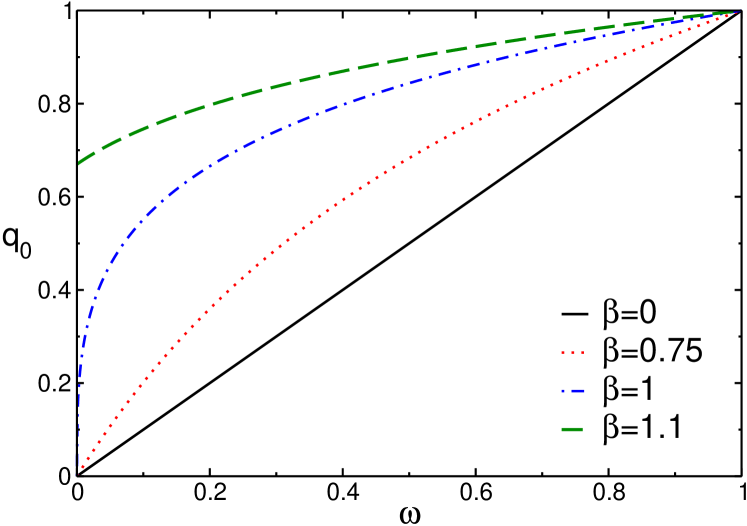
Figure 2: The S-K model on the $2$-sheets booklet in the paramagnetic phase: the solution $q_{0}$ of the saddle point equation (34) plotted as a function of the booklet aspect ratio $\omega$ and several values of the inverse temperature $\beta=1/T$. At $\omega=1$ one has $q_{0}=1,\forall\beta$. In the zero-temperature limit one has $q_{0}\to 1,\forall\omega$. The straight line is the infinite temperature result.

Here we provide the exact analytical expression for the disorder-averaged free energy $[F_{para}(\omega,n,\beta)]$ in the paramagnetic non-glassy phase. We start discussing the infinite temperature limit (i.e., $\beta\to 0$), restricting ourselves to zero magnetic field. Using Eq. (17), a standard high-temperature expansion yields $\textrm{Tr}_{A}e^{{\mathcal{L}}}=2^{\alpha}+{\mathcal{O}}(\beta^{2})$ and $\textrm{Tr}_{B}e^{{\mathcal{L}}}=2^{n\alpha}+{\mathcal{O}}(\beta^{2})$, implying

$$\langle S^{(r,\gamma)}S^{(r^{\prime},\gamma^{\prime})}\rangle_{B}=2^{n\alpha}\delta_{\gamma,\gamma^{\prime}}\delta_{r,r^{\prime}}+{\mathcal{O}}(\beta^{2})$$ (24)

$$\langle S^{(r,\gamma)}S^{(r^{\prime},\gamma^{\prime})}\rangle_{A}=2^{\alpha}\delta_{\gamma,\gamma^{\prime}}+{\mathcal{O}}(\beta^{2}).$$ (25)

Using Eq. (22), it is straightforward to obtain the infinite-temperature overlap tensor $q_{\gamma\gamma^{\prime}}^{rr^{\prime}}$ as

$$q_{\gamma\gamma^{\prime}}^{rr^{\prime}}=(1-\omega)\delta_{\gamma,\gamma^{\prime}}\delta_{r,r^{\prime}}+\omega\delta_{\gamma,\gamma^{\prime}}.$$ (26)

Notice that $q_{\gamma\gamma^{\prime}}^{rr^{\prime}}$ is diagonal in both the indices $\gamma,\gamma^{\prime}$ and $r,r^{\prime}$, i.e., the sheet and the replica spaces. Using Eq. (19) and Eq. (12), after performing the analytic continuation $\alpha\to 0$, one obtains

$$[F_{para}(\omega,n,\beta)]=N\Big{\{}(n-\omega(n-1))\log(2)\\ +\frac{\beta^{2}}{4}(\omega^{2}(n^{2}-n)+n)\Big{\}}+{\mathcal{O}}(\beta^{4}).$$ (27)

It is natural to expect that for finite $\beta\leq\beta_{c}$, with $\beta_{c}$ the critical temperature of the paramagnetic-glassy transition, the overlap tensor $q_{\gamma\gamma^{\prime}}^{rr^{\prime}}$ remains diagonal. This suggests the ansatz

$$q_{\gamma\gamma^{\prime}}^{rr^{\prime}}=(1-q_{0})\delta_{r,r^{\prime}}\delta_{\gamma,\gamma^{\prime}}+q_{0}\delta_{\gamma,\gamma^{\prime}}.$$ (28)

with $q_{0}\in{\mathbb{R}}$ a parameter. The ansatz (28) is formally obtained from Eq. (26) by replacing $\omega\to q_{0}$. Notice that one has $q_{\gamma\gamma}^{rr}=1$, in agreement with Eqs. (22). Using Eq. (28), one obtains ${\mathcal{L}}_{para}$ (cf. Eq. (17)) as

$${\mathcal{L}}_{para}=\beta^{2}\frac{q_{0}}{2}\Big{\{}\sum_{\gamma}\sum_{rr^{\prime}}S^{(r,\gamma)}S^{(r^{\prime},\gamma)}-n\alpha\Big{\}}.$$ (29)

After introducing the Hubbard-Stratonovich variables $z_{\lambda}$ (with $\lambda=1,\dots,\alpha$), one can write

$$\textrm{Tr}_{B}\exp({\mathcal{L}}_{para})=\\ \textrm{Tr}_{B}\int\prod_{\lambda}Dz_{\lambda}\exp\Big{(}z_{\lambda}\beta\sqrt{q_{0}}\sum_{r}S^{(r,\lambda)}\Big{)},$$ (30)

where $\int Dzf(z)\equiv(2\pi)^{-1/2}\int\exp(-z^{2}/2)f(z)$. Notice that due to the square root in Eq. (30), one has the constraint $q_{0}>0$. Moreover, from Eq. (29) one obtains $\textrm{Tr}_{A}\exp({\mathcal{L}})=2^{n\alpha}$. The trace $\textrm{Tr}_{B}$ in Eq. (30) can be performed explicitly. Using Eq. (19) and Eq. (12), one obtains the free energy $[F_{para}(\omega,n,\beta)]$ as

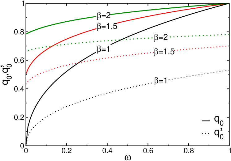
Figure 3: The S-K model on the $2$-sheets booklet. The overlap tensor in the replica-symmetric (RS) approximation (see Eq. (37)): the solutions $q_{0}$ and $q_{0}^{\prime}$ (shown as full and dotted lines, respectively) of the saddle point equations (58)(59) plotted as a function of the booklet aspect ratio $\omega$, and inverse temperature $\beta=1/T=1,3/2,2$. At $\omega=1$ one has that $q_{0}=1,\forall\beta$. In the limit $\beta\to\infty$ it is $q_{0},q_{0}^{\prime}\to 1,\forall\omega$.

$$[F_{para}(\omega,n,\beta)]=N\Big{\{}n\log(2)-\omega(n-1)\log(2)\\ +\frac{\beta^{2}}{2}\Big{(}\frac{n}{2}-\frac{q_{0}^{2}}{2}(n^{2}-n)+\omega q_{0}n^{2}-q_{0}n\Big{)}\\ +(1-\omega)\log\int Dz\cosh^{n}(z\sqrt{q_{0}}\beta)\Big{\}},$$ (31)

where $q_{0}$ is determined by solving the saddle point condition $\partial[F_{para}(\omega,n,\beta)]/\partial q_{0}=0$. $[F_{para}(\omega,n,\beta)]$ can be written in terms of simple functions using that

$$\frac{1}{\sqrt{2\pi}}\int Dz\cosh^{n}(z\sqrt{q_{0}}\beta)=\\ \frac{1}{2^{n-1}}\sum\limits_{k=0}^{\lfloor n/2\rfloor-1}\frac{\Gamma(n+1)}{\Gamma(k+1)\Gamma(n-k+1)}e^{2\beta^{2}q_{0}(n/2-k)^{2}}\\ +\frac{2^{-2\left\lfloor n/2\right\rfloor}\Gamma(n+1)}{\Gamma(n-\lfloor n/2\rfloor+1)\Gamma(\lfloor n/2\rfloor+1)}e^{2\beta^{2}q_{0}(n/2-\lfloor n/2\rfloor)^{2}},$$ (32)

where $\Gamma(x)$ denotes the Euler Gamma function. The saddle point equation for $q_{0}$ reads

$$0=\beta\big{(}\omega n-1-q_{0}(n-1)\big{)}\\ +(1-\omega)\frac{\int Dz\cosh^{n-1}(z\sqrt{q_{0}}\beta)\sinh(z\sqrt{q_{0}}\beta)z}{\sqrt{q_{0}}\int Dz\cosh^{n}(z\sqrt{q_{0}}\beta)}.$$ (33)

For the $2$-sheets booklet (i.e., $n=2$) this is given as

$$q_{0}=\omega+(1-\omega)\tanh(\beta^{2}q_{0}).$$ (34)

Alternatively, Eq. (34) can be obtained by substituting the ansatz (28) in Eqs. (22) (23). Clearly, for two independent copies of the S-K model, i.e., $\omega=0$, Eq. (34) gives $q_{0}=0$ for $\beta\leq 1$, whereas one has $q_{0}\neq 0$ for $\beta>1$. On the other hand, for $\omega=1$ one has $q_{0}=1$ $\forall\beta$. For intermediate $0<\omega<1$, $q_{0}$ is plotted as a function of $\omega$ in Fig. 2. For $\beta=0$ it is $q_{0}=\omega$ (straight line in the Figure). In the low-temperature limit one has $q_{0}\to 1$, for any $\omega$. In particular, it is straightforward to check that $q_{0}\approx 1-2(1-\omega)\exp(-2\beta^{2})$ for $\beta\to\infty$.

IV.2 The analytic continuation $n\to 1$

It is interesting to consider the analytic continuation $\lim_{n\to 1}[S_{n}]$ and $\lim_{n\to 1}[{\mathcal{I}}_{n}]$ to obtain the Shannon entropy and mutual information. In the limit $n\to 1$, $F_{para}(\omega,n,\beta)$ (see (31)) does not depend on $q_{0}$ and $\omega$, as expected. This holds for any $\beta$ even including the effects of the replica symmetry breaking. However, the Shannon entropy $S_{1}(A)$ (and the mutual information ${\mathcal{I}}_{1}$ thereof) is non trivial due to the prefactor $1/(1-n)$ in (5). In order to obtain $S_{1}(A)$ one should consider $1/(1-n)[F_{para}(\omega,n,\beta)]$ performing carefully the limit $n\to 1$. The result reads

$$\frac{[F_{para}(\omega,1,\beta)]}{N(1-n)}=\omega\log(2)+\frac{\beta^{2}}{2}\Big{(}\frac{q_{0}^{2}}{2}n-\omega q_{0}(n+1)+q_{0}\Big{)}\\ -(1-\omega)\frac{\int Dz\cosh(z\sqrt{q_{0}}\beta)\log\cosh(z\sqrt{q_{0}}\beta)}{\int Dz\cosh(z\sqrt{q_{0}\beta})}.$$ (35)

The saddle point equation (33) for $q_{0}$ now becomes

$$(\omega-q_{0})\exp\big{(}\beta^{2}\frac{q_{0}}{2}\big{)}+(1-\omega)\int Dz\Big{(}\frac{z}{\beta\sqrt{q_{0}}}\sinh(z\sqrt{q_{0}}\beta)\\ -\cosh(z\sqrt{q_{0}}\beta)\Big{)}\log\cosh(z\sqrt{q_{0}}\beta)=0.$$ (36)

Notice that in the limit $\beta\to 0$ one has $q_{0}\to\omega$, which implies, using (35) and (4), the volume-law behavior $[{\mathcal{I}}_{1}]\to\beta^{2}/2\omega(1-\omega)N$. This in constrast with the clean case wilms-2012 , where ${\mathcal{I}}_{1}={\mathcal{O}}(1)$ for any $\beta$ away from the critical point at $\beta_{c}=1$.

IV.3 The replica-symmetric (RS) approximation

In the replica-symmetric (RS) approximation one writes the overlap tensor $q_{\gamma\gamma^{\prime}}^{rr^{\prime}}$ as

$$q_{\gamma\gamma^{\prime}}^{rr^{\prime}}=(1-q_{0})\delta_{r,r^{\prime}}\delta_{\gamma,\gamma^{\prime}}+q_{0}\delta_{\gamma,\gamma^{\prime}}+(1-\delta_{\gamma,\gamma^{\prime}})q^{\prime}_{0}.$$ (37)

The first two terms in Eq. (37) are the same as in the paramagnetic phase (cf. Eq. (28)). The last term sets $q_{\gamma\gamma^{\prime}}^{rr^{\prime}}=q^{\prime}_{0}$ $\forall\gamma\neq\gamma^{\prime}$ and $\forall r,r^{\prime}$. Clearly, $q_{\gamma\gamma^{\prime}}^{rr^{\prime}}$ is invariant under permutations of both the booklet sheets and the replicas. We do not have any rigorous argument to justify the ansatz (37), besides its simplicity. However, we numerically observe that it captures quite accurately the behavior of the model, at least around the paramagnetic-glassy transition (see section VI for the comparison with Monte Carlo data).

Using Eq. (37) and Eqs. (12)(19) one obtains the replica-symmetric approximation for the free energy $[F_{RS}(\omega,n,\beta)]$ as

$$[F_{RS}(\omega,n,\beta)]=\\ \lim_{\alpha\to 0}\Big{\{}N\Big{[}\frac{\beta^{2}}{4}n-\frac{\beta^{2}}{4}\Big{(}(q_{0}^{2}-(q^{\prime}_{0})^{2})n^{2}-q_{0}^{2}n\Big{)}\\ +\frac{1-\omega}{\alpha}\log\textrm{Tr}_{B}\exp({\mathcal{L}}_{RS})\\ +\frac{\omega}{\alpha}\log\textrm{Tr}_{A}\exp({\mathcal{L}}_{RS})\Big{]}\Big{\}},$$ (38)

where ${\mathcal{L}}_{RS}$ is obtained by substituting Eq. (37) in Eq. (17), which yields

$${\mathcal{L}}_{RS}=\frac{q_{0}^{\prime}}{2}\beta^{2}\sum\limits_{\gamma\gamma^{\prime}}\sum_{rr^{\prime}}S^{(r,\gamma)}S^{(r^{\prime},\gamma^{\prime})}\\ +\frac{q_{0}-q_{0}^{\prime}}{2}\beta^{2}\sum_{\gamma}\sum_{rr^{\prime}}S^{(r,\gamma)}S^{(r^{\prime},\gamma^{\prime})}-\frac{q_{0}}{2}\beta^{2}n\alpha.$$ (39)

To calculate the last two terms in Eq. (38) one has to introduce two auxiliary Hubbard-Stratonovich variables $z,z^{\prime}$, similar to the paramagnetic phase (cf. section IV.1). Thus, after performing the trace over the spin variables, in the limit $\alpha\to 0$, one obtains

$$\log\textrm{Tr}_{B}\exp({\mathcal{L}}_{RS})= -\frac{q_{0}}{2}\beta^{2}n\alpha+n\alpha\log(2)$$ (40)

$$+\alpha\int Dz\log\int Dz^{\prime}H_{RS}^{n}(z,z^{\prime}),$$

$$\log\textrm{Tr}_{A}\exp({\mathcal{L}}_{RS})= -\frac{q_{0}}{2}\beta^{2}n\alpha+\alpha\log(2)$$ (41)

$$+\alpha\int Dz\log\int Dz^{\prime}H_{RS}(nz,nz^{\prime}),$$

where $H_{RS}(z,z^{\prime})\equiv\cosh(\beta z\sqrt{q_{0}^{\prime}}+\beta z^{\prime}\sqrt{q_{0}-q_{0}^{\prime}})$. Notice that because of the square roots in the definition of $H_{RS}(z,z^{\prime})$, one has the constraint $0\leq q_{0}^{\prime}\leq q_{0}\leq 1$.

In Eqs. (40)(41) $q_{0},q_{0}^{\prime}$ satisfy the saddle point conditions $\partial[F_{RS}(\omega,n,\beta)]/\partial q_{0}=\partial[F_{RS}(\omega,n,\beta)]/\partial q^{\prime}_{0}=0$ (cf. Eqs. (58)(59) for their form for $n=2$). The resulting $q_{0}$ and $q_{0}^{\prime}$ are plotted in Fig. 3 (full and dotted lines, respectively) as function of $\omega$ and for several values of $\beta$. Clearly, for any $\beta$ one has $q_{0}=1$ in the limit $\omega\to 1$. Also, in the zero-temperature limit $\beta\to\infty$ one has that $q_{0}\to 1$ and $q_{0}^{\prime}\to 1$, for any $\omega$. Moreover, a simple large $\beta$ expansion yields

$$q_{0}=1-(1-\omega)\sqrt{\frac{2}{\pi}}\frac{1}{\beta}\exp\Big{(}-\frac{1}{\pi}-\sqrt{\frac{2}{\pi}}\beta\Big{)}+\dots$$ (42)

$$q_{0}^{\prime}=1-\frac{1}{\sqrt{2\pi}\beta}-\frac{1}{2\pi\beta^{2}}+{\mathcal{O}}(\beta^{-3}),$$ (43)

with the dots denoting exponentially suppressed terms in the limit $\beta\to\infty$. Interestingly, from Eq. (42) one has that $q_{0}\to 1$ exponentially in the limit $\beta\to\infty$, as in the paramagnetic phase (cf. section IV.1), whereas $q_{0}^{\prime}-1\propto 1/\beta$.

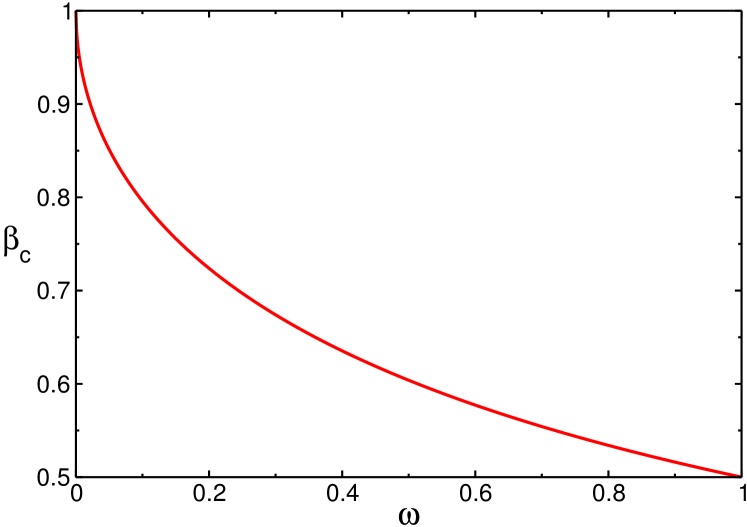
Figure 4: The critical temperature $\beta_{c}\equiv 1/T_{c}$ of the paramagnetic-glassy transition for the S-K model on the $2$-sheets booklet (see Fig. 1) from Eq. (44): $\beta_{c}$ as a function of the booklet ratio $\omega\equiv N_{A}/N$. Here $\beta_{c}$ is obtained from the replica-symmetric (RS) approximation. Notice that $\beta_{c}=1$ and $\beta_{c}=1/2$ for $\omega=0$ and $\omega=1$, respectively.

IV.4 The paramagnetic-glassy transition

Using the replica-symmetric ansatz Eq. (37) one can determine the critical temperature $\beta_{c}$ of the paramagnetic-glassy transition. Near the glassy transition one should expect $q^{\prime}_{0}\to 0$, whereas $q_{0}$ should remain finite (see section IV.1). One expands $[F_{RS}(\omega,n,\beta)]$ (cf. Eq (38)) for small $q_{0}^{\prime}$, keeping only terms up to ${\mathcal{O}}((q_{0}^{\prime})^{2})$. Thus, $\beta_{c}$ is obtained by imposing that the coefficient of the quadratic term $q_{0}^{\prime 2}$ vanishes. This leads to the equation

$$\exp(-4q_{0}\beta^{2}_{c})+2\exp(-2q_{0}\beta^{2}_{c})=\frac{1-4\beta^{2}_{c}}{4\beta^{2}_{c}\omega-1},$$ (44)

where $q_{0}$ is obtained by solving the high-temperature saddle point equation (34). The resulting $\beta_{c}$ is plotted in Fig. 4 as a function of $\omega$.

V The one-step replica-symmetry-breaking (1-RSB) approximation

In this section we go beyond the replica-symmetric approximation, including some of the effects of the replica symmetry breaking. More specifically, here we discuss the one-step replica symmetry breaking (1-RSB) approximation. The overlap tensor $q_{\gamma\gamma^{\prime}}^{rr^{\prime}}$ now reads

$$q_{\gamma\gamma^{\prime}}^{rr^{\prime}}=(1-q_{0})\delta_{\gamma,\gamma^{\prime}}\delta_{r,r^{\prime}}+q_{0}\delta_{\gamma,\gamma^{\prime}}+(1-\delta_{\gamma,\gamma^{\prime}})q^{\prime},$$ (45)

which is formally equivalent to the RS ansatz in Eq. (37), apart from the trivial redefinition $q_{0}^{\prime}\to q^{\prime}$. However, in contrast with Eq. (37), where $q_{0}^{\prime}\in\mathbb{R}$ is a number, here $q^{\prime}$ is a matrix. Inspired by the Parisi scheme for the standard S-K model parisi-1979 , we choose

$$q^{\prime}=\left\{\begin{array}[]{cc}q_{1}^{\prime}&\textrm{if}\,\lfloor\gamma/m_{1}\rfloor=\lfloor\gamma^{\prime}/m_{1}\rfloor\\ \\ q_{0}^{\prime}&\textrm{otherwise}\\ \end{array}\right.$$ (46)

where $q_{0}^{\prime},q_{1}^{\prime}\in{\mathbb{R}}$, $m_{1}\in{\mathbb{N}}$, and $\lfloor\cdot\rfloor$ denotes the floor function. Notice that the off-diagonal elements of $q^{\prime}$ (i.e., for $\gamma\neq\gamma^{\prime}$) do not depend on $r,r^{\prime}$, meaning that, although the permutation symmetry between the replicas is broken, the symmetry among the booklet sheets is preserved. The choice in Eq. (46) corresponds to a simple block-diagonal structure for $q^{\prime}$: the matrix elements of the $m_{1}\times m_{1}$ diagonal blocks of $q^{\prime}$ are set to $q_{1}^{\prime}$, whereas all the off-diagonal elements are set to $q_{0}^{\prime}$. As for the replica-symmetric ansatz in Eq. (37), we do not have any rigorous argument to justify Eq. (46) (see section (VI), however, for numerical results).

The effective interaction ${\mathcal{L}}_{1\textrm{-}RSB}$ (cf. Eq. (17)) in the replica space is obtained by substituting Eq. (45) in Eq. (17). This yields

$${\mathcal{L}}_{1\textrm{-}RSB}/\beta^{2}=-\frac{q_{0}}{2}n\alpha-\frac{q_{1}^{\prime}-q_{0}}{2}\sum\limits_{\sigma=1}^{\alpha/m_{1}}\sum\limits_{\gamma\in B_{\sigma}}\Big{(}\sum_{r}S^{(r,\gamma)}\Big{)}^{2}\\ +\frac{q_{0}^{\prime}}{2}\Big{(}\sum\limits_{\gamma,r}S^{(r,\gamma)}\Big{)}^{2}-\frac{q_{0}^{\prime}-q_{1}^{\prime}}{2}\sum\limits_{\sigma=1}^{\alpha/m_{1}}\Big{(}\sum\limits_{\gamma\in B_{\sigma},r}S^{(r,\gamma)}\Big{)}^{2},$$ (47)

where we defined $B_{\sigma}\equiv[\sigma m_{1},(\sigma+1)m_{1})$ with $\sigma\in\mathbb{N}$.

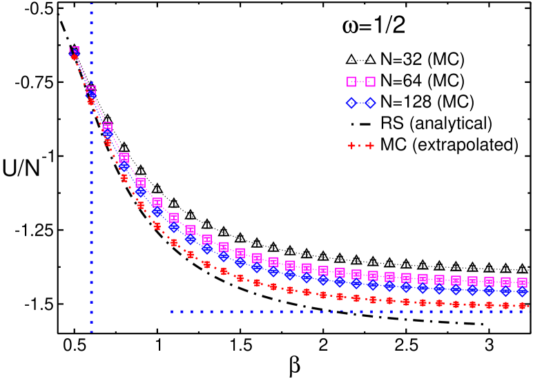
Figure 5: The S-K model on the $2$-sheets booklet with aspect ratio $\omega=1/2$ (see Fig. 1): The internal energy per spin $U/N$ as a function of the inverse temperature $\beta$. The triangles, squares, and rhombi, denote the Monte Carlo data for a booklet with $N=32,64,128$ spins per sheet. Notice that the Monte Carlo error bars are often smaller than the symbol sizes. The plus symbols are the extrapolations to the thermodynamic limit $N\to\infty$, at fixed $\omega$. The dash-dotted line is the analytical result $U_{RS}/N$ obtained using the replica-symmetric (RS) approximation. The horizontal dotted line is the exact zero-temperature result $U/N=2u_{\infty}$, with $\tilde{u}_{\infty}\approx-0.76321$ the zero temperature energy density of the regular S-K model parisi-1979 ; parisi-1983 .

It is convenient to introduce the Hubbard-Stratonovich variables $z,z_{\sigma},z_{\sigma,\gamma}$ (one for each term in Eq. (47)). One then obtains

$$\log\textrm{Tr}^{\prime}\exp({\mathcal{L}}_{1\textrm{-}RSB})=-\frac{q_{0}}{2}\beta^{2}n\alpha\\ +\log\textrm{Tr}^{\prime}\int Dz\prod_{\sigma}\int Dz_{\sigma}\prod\limits_{\gamma\in B_{\sigma}}\int Dz_{\sigma,\gamma}\prod_{r}\exp\Big{\{}\\ \beta\Big{(}z\sqrt{q^{\prime}_{0}}+z_{\sigma,\gamma}\sqrt{q_{0}-q_{1}^{\prime}}+z_{\sigma}\sqrt{q_{1}^{\prime}-q_{0}^{\prime}}\Big{)}S^{(r,\gamma)}\Big{\}}.$$ (48)

The trace over the spin variables in Eq. (48) can be now performed explicitly. Finally, one obtains the 1-RSB approximation for the free energy $[F_{1\textrm{-}RSB}(\omega,n,\beta)]$ as

$$[F_{1\textrm{-}RSB}(\omega,n\beta)]/N=(\omega+(1-\omega)n)\log(2)+\frac{n}{4}\beta^{2}\Big{(}1+nq_{0}^{\prime 2}-n(m_{1}-1)(q_{1}^{\prime 2}-q_{0}^{\prime 2})-(n-1)q_{0}^{2}-2q_{0}\Big{)}\\ +\int Dz\left\{\frac{1-\omega}{m_{1}}\log\int Dz^{\prime}\Big{\{}\int Dz^{\prime\prime}H_{1\textrm{-}RSB}^{n}(z,z^{\prime},z^{\prime\prime})\Big{\}}^{m_{1}}+\frac{\omega}{m_{1}}\log\int Dz^{\prime}\Big{\{}\int Dz^{\prime\prime}H_{1\textrm{-}RSB}(nz,nz^{\prime},nz^{\prime\prime})\Big{\}}^{m_{1}}\right\},$$ (49)

where we defined $H_{1\textrm{-}RSB}(z,z^{\prime},z^{\prime\prime})$ as

$$H_{1\textrm{-}RSB}(z,z^{\prime},z^{\prime\prime})\equiv\cosh(z\beta\sqrt{q^{\prime}_{0}}\\ +z^{\prime\prime}\beta\sqrt{q_{0}-q^{\prime}_{1}}+z^{\prime}\beta\sqrt{q_{1}^{\prime}-q_{0}^{\prime}}).$$ (50)

Similar to the replica-symmetric situation (see section IV.3), from Eq. (50) one has the constraint $0\leq q_{0}^{\prime}\leq q_{1}^{\prime}\leq q_{0}\leq 1$. The parameters $q_{0},q_{0}^{\prime},q_{1}^{\prime},m_{1}$ are obtained by solving the saddle point equations (64)(65)(66) (67). One should remark that, although $m_{1}$ is by defintion an integer, one obtains $m_{1}\in\mathbb{R}$ from the saddle point equations. Clearly, the replica-symmetric result $[F_{RS}(\omega,n,\beta)]$ (cf. Eq. (38)) is recovered from Eq. (49) in the limit $q_{1}^{\prime}=q_{0}^{\prime}$, while the free energy in the paramagnetic phase $[F_{para}(\omega,n,\beta)]$ (cf. Eq. (31)) corresponds to $q_{1}^{\prime}=q_{0}^{\prime}=0$.

VI Monte Carlo results: The internal energy

In this section we numerically confirm the analytical results of section IV. We discuss Monte Carlo (MC) data for the S-K model on the $2$-sheets booklet with zero external magnetic field. The data we present are obtained from parallel tempering Monte Carlo simulations hukushima-1996 . In the parallel tempering simulations $N_{\textrm{rep}}$ identical disorder realizations of the system are simulated. Each copy is at a different temperature in the range $\beta_{\textrm{min}}-\beta_{\textrm{max}}$. The standard Metropolis sweeps at each temperature are supplemented with parallel tempering moves, which allow to exchange the spin configurations between replicas with neighboring temperatures. In our simulations we choose the interval with $\beta_{\textrm{min}}=0.25$ and $\beta_{\textrm{max}}=2.5$, with $46$ temperatures corresponding to equally spaced values of $\beta$. Each Monte Carlo sweep consists of $N$ single spin updates and $45$ parallel tempering moves. For each disorder realization we perform $10^{5}$ sweeps. The disorder average is performed over $128$ different disorder realizations.

We focus on the internal energy $U(\omega,n,\beta)$

$$U(\omega,n,\beta)\equiv-\frac{\partial}{\partial\beta}[\log(Z(\omega,n,\beta))].$$ (51)

Fig. 5 plots the MC data for $U(\omega,2,\beta)$ versus the inverse temperature $\beta$, for $\omega=1/2$. The circles, squares, and triangles are the MC results for different sizes, i.e., number of spins per sheet, $N=32,64,128$. The vertical dotted line is the critical temperature $\beta_{c}\approx 0.6$ of the paramagnetic-glassy transition (cf. Fig. 4). In the high-temperature region finite-size effects are small, and already for $N=64$ the MC data are indistinguishable from the thermodynamic limit result. Oppositely, stronger scaling corrections are visible in the low-temperature phase at $\beta>\beta_{c}$. The plus symbols in Fig. 5 are the numerical extrapolations in the thermodynamic limit. These are obtained by fitting the finite size MC data to the ansatz $U/N=u_{\infty}(\omega,\beta)+c/N^{\phi}$, where $u_{\infty}$ is energy density in the thermodynamic limit, $c$ a fitting parameter, and $\phi$ the exponent of the scaling corrections. In our fits we fix $\phi=2/3$, which is the exponent governing the finite-size corrections of $U/N$ in the standard S-K model billoire-2007 ; aspelmeier-2008 .

The dash-dotted line in Fig. 5 is the analytical result $U_{RS}$ obtained using the replica-symmetric (RS) approximation (see section IV.3). Using Eq. (38) and Eq. (51), $U_{RS}$ is obtained as

$$U_{RS}=-N\beta(1+q_{0}^{2}-2q_{0}^{\prime 2}).$$ (52)

Here $q_{0},q_{0}^{\prime}$ are solutions of the saddle point equations Eqs. (58) (59). Notice that $U_{RS}$ depends on $\omega$ only through $q_{0},q_{0}^{\prime}$. From Fig. 5 one has that, while $U_{RS}$ is in perfect agreement with the numerics for $\beta\approx\beta_{c}$, deviations appear in the low-temperature region. Notice that already at $\beta\gtrsim 1$, $U_{RS}$ is incompatible with the data. These deviations increase upon lowering the temperature and have to be attributed to the replica symmetry breaking happening in the glassy phase. Finally, since in the limit $\beta\to\infty$ all the sheets are in the same state, one should expect that $u_{\infty}(\omega,\beta)\to n\tilde{u}_{\infty}$ (horizontal line in Fig. 5), with $\tilde{u}_{\infty}=-0.76321...$ parisi-1979 ; parisi-1983 the zero-temperature internal energy density of the S-K model on the plane.

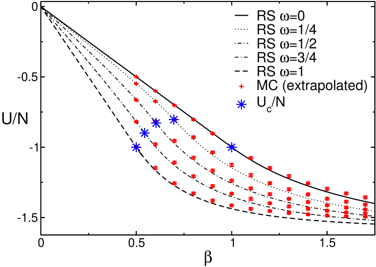
Figure 6: The S-K model on the 2-sheets booklet: The internal energy per spin $U/N$ in the thermodynamic limit. The symbols are the Monte Carlo data extrapolated to the thermodynamic limit $N\to\infty$, at fixed booklet ratio $\omega$ (see Fig. 1). $U/N$ is plotted as a function of inverse temperature $\beta$ and for $\omega=0,1/4,1/2,3/4,1$. The lines are the analytical results $U_{RS}$ obtained using the replica-symmetric (RS) approximation. The stars denote the value of $U_{c}/N$ at the paramagnetic-glassy transition.

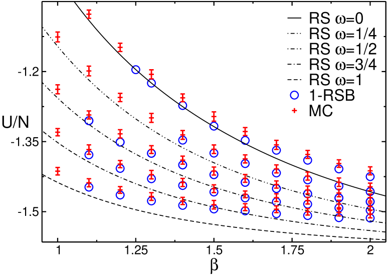
Figure 7: The S-K model on the 2-sheets booklet: The internal energy per spin $U/N$ in the thermodynamic limit plotted as a function of inverse temperature $\beta$. The plus symbols are the same extrapolated Monte Carlo data as in Fig. 6. The lines denote $U/N$ in the replica-symmetric (RS) approximation (same as in Fig. 6). The circles are the results in the one-step replica symmetry breaking (1-RSB) approximation.

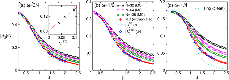
Figure 8: The classical disorder-averaged Rényi entropy per spin $[S_{2}(\omega)]/N$ in the S-K model on the $2$-sheets booklet: $[S_{2}(\omega)]/N$ as a function of the inverse temperature $\beta$. The different panels correspond to different booklet aspect ratios $\omega=3/4,1/2,1/4$ (see Fig. 1). The triangles, squares and rhombi denote the Monte Carlo results for booklets with $N=32,64,128$ spins per sheet. The Monte Carlo error bars are often smaller than the symbol size. The plus symbols are the numerical extrapolations to the thermodynamic limit. The inset in panel (a) shows $[S_{2}]/N$ at fixed $\beta=2$, plotted versus $N^{-2/3}$.The dotted line is a linear fit. In all the panels the dash-dotted lines are the analytical results in the replica-symmetry (RS) approximation. The circles are the analytical results obtained using the one-step replica symmetry breaking (1-RSB) ansatz. In panel (c) the dotted line (clean Ising) is the analytic result for the infinite-range Ising model without disorder.

The behavior of $U/N$ for different $\omega$ is investigated in Fig. 6, plotting $U/N$ as a function of $\beta$ and for $\omega=0,1/4,3/4,1$. The result for $\omega=1/2$ is shown for comparison. The plus symbols are the MC data extrapolated to the thermodynamic, at fixed $\omega$. Similar to Fig. 6, the extrapolations are done assuming $U/N(\omega,n,\beta)=u_{\infty}(\omega,n,\beta)+c/N^{\phi}$, with $\phi=2/3$ irrespective of $\omega$. The stars in Fig. 6 are the critical values $U_{c}/N$ at the paramagnetic-glassy transition, whereas the lines are the analytical results (cf. Eq. (52)). Notice that at high temperature, and for generic $n$ and $\omega$, Eq. (27) and Eq. (51) give

$$U_{RS}=-N\frac{\beta}{2}(\omega^{2}(n^{2}-n)+n)+{\mathcal{O}}(\beta^{2}),$$ (53)

i.e., a linear behavior of $U/N$ as a function of $\beta$. For $\omega=0$ and $\omega=1$ this behavior is exact up to the critical point at $\beta=\beta_{c}$, meaning that the higher orders ${\mathcal{O}}(\beta^{2})$ in Eq. (53) are zero. This is only an approximation at intermediate $0<\omega<1$. Both the behaviors in Eq. (52) and Eq. (53) are clearly confirmed in Fig. 6.

However, from Fig. 6 one has that the RS result is not correct for $\beta>\beta_{c}$, where the replica symmetry breaking has to be taken into account. This is more carefully discussed in Fig. 7, focusing on the low temperature region at $1\leq\beta\leq 2$. The plus symbols and the lines are the same as in Fig. 6. The circles denote the internal energy per spin $U_{1\textrm{-}RSB}/N$ as obtained using the $1$-step replica symmetry breaking (1-RSB) approximation (see section V). Specifically, from Eq. (49) and Eq. (51), for $n=2$ a straightforward calculation gives

$$U_{1\textrm{-}RSB}=-N\beta(1+q_{0}^{2}+2q_{1}^{\prime 2}(m_{1}-1)-2q_{0}^{\prime 2}m_{1}),$$ (54)

where $q_{0},q_{0}^{\prime},q_{1}^{\prime},m_{1}\in\mathbb{R}$ are solutions of the saddle point equations (64)-(67). Clearly, Eq. (54) implies $U_{1\textrm{-}RSB}\to U_{RS}$ for $q_{1}^{\prime}\to q_{0}^{\prime}$, as expected. Moreover, for $\beta\approx\beta_{c}$ one has $q_{1}^{\prime}\approx q_{0}^{\prime}\approx 0$, implying that $U_{1\textrm{-}RSB}\approx U_{RS}$, i.e. the effects of the replica symmetry breaking are negligible near the critical point. Interestingly, at low temperatures, where the RS approximation fails (see Fig. 6), $U_{1\textrm{-}RSB}$ is in good agreement with the Monte Carlo data, at least up to $\beta\approx 2$.

VII The classical Rényi entropies

We now turn to discuss the behavior of the classical Rényi entropies (cf. Eq. (5)). Here we restrict ourselves to the second Rényi entropy $[S_{2}]$, which is obtained in terms of the booklet partition function $Z(\omega,2,\beta)$ (see section II) as $-\log(Z(\omega,2,\beta)/Z(0,2,\beta))$. Due to the mean-field nature of the S-K model (cf. Eq. (7)), there is no well defined boundary between the two parts $A$ and $B$ of the system (unlike in local spin models). With this in mind we assume that we will find volume law behavior $[S_{2}]\propto N$, and consider the entropy per spin $[S_{2}]/N$ as the quantity of interest.

Figure 9: The classical disorder-averaged mutual information per spin $[{\mathcal{I}}_{2}]/N$ in the S-K model on the $2$-sheets booklet: $[{\mathcal{I}}_{2}]/N$ versus the inverse temperature $\beta$. The different panels correspond to different booklet ratios $\omega=1/2,1/4,1/8$ (see Fig. 1). The same scale is used on both axes in all panels. The symbols are the Monte Carlo data for systems with $N=32,64,128$ spins per sheet. The Monte Carlo error bars are smaller than the symbol size. The dash-dotted line is the analytical result in the replica-symmetric (RS) approximation. In (a) the dotted line is the result for the clean, i.e., without disorder, infinite-range Ising model.

The Monte Carlo data for $[S_{2}]/N$ are shown in Fig. 8 plotted versus the inverse temperature $0.25\leq\beta\leq 2.5$. Some details on the Monte Carlo method used to calculate $[S_{2}]$ are provided in Appendix C. The different panels correspond to the booklet ratios $\omega=3/4,1/2,1/4$ (see Fig. 1). In all the panels the triangles, squares, and rhombi correspond to booklets with $N=32,64,128$ spins per sheet. Clearly, finite size effects are present, which increase upon lowering the temperature, as expected. In order to obtain $[S_{2}]/N$ in the thermodynamic limit we fit the data to the ansatz $[S_{2}]/N=s_{2}(\omega)+c^{\prime}(\omega)/N^{\phi}$, where $s_{2}(\omega)$ is the entropy per spin in the thermodynamic limit, $c^{\prime}$ a constant, and $\phi$ the exponent of the finite-size corrections. The plus symbols in Fig. 8 are the results of the fits. We should mention that the fits give $\phi\approx 2/3$, which is the exponent of the scaling corrections of the free energy in the standard S-K model. This is not surprising, since $[S_{2}]$ is obtained as the difference $[S_{2}]\equiv[F(0,2,\beta)-F(\omega,2,\beta)]$ (cf. Eq. (5)). Clearly, from Fig. 8 one has that in the thermodynamic limit $[S_{2}]/N$ is finite for any $\beta$, confirming the expected volume law behavior. Moreover, $[S_{2}]/N$ exhibits a maximum in the infinite-temperature limit $\beta\to 0$. The height of this maximum is a decreasing function of $\omega$ (compare the panels (a)(b)(c) in Fig. 8).

The dash-dotted line in the Figure denotes the analytical result $[S_{2}^{RS}]$ obtained within the RS approximation (see section IV.3). More precisely, $[S_{2}^{RS}]/N$ is obtained from Eq. (5) and the expression for the free energy $[F_{RS}]$ (cf. Eq. (38)). Notice that in the high-temperature limit $\beta\to 0$, where the RS approximation is exact, Eq. (5) and Eq. (31) give

$$\frac{[S^{RS}_{2}]}{N}=\omega\log(2)-\frac{\beta^{2}}{4}\omega^{2}+{\mathcal{O}}(\beta^{3}).$$ (55)

From Fig. 8 one has that the extrapolated MC data are in quantitative agreement with $[S_{2}^{RS}]/N$ for $\beta\lesssim 1.5$, whereas strong deviations are observed at lower temperatures (not shown in the Figure). A better approximation for $[S_{2}]/N$ at low temperatures is obtained by including the effects of the replica symmetry breaking. The circles in Fig. 8 denote the one-step replica symmetry breaking result $[S_{2}^{1\textrm{-}RSB}]/N$ (see section V), which is obtained from Eq. (5) and Eq. (49). Remarkably, $[S_{2}^{1\textrm{-}RSB}]/N$ is in excellent agreement with the extrapolated Monte Carlo data for $\beta\lesssim 2$. Finally, for comparison we report in panel (c) the analytical result (dotted line) for $S_{2}/N$ for the infinite-range Ising model without disorder at $\omega=1/4$ (see Appendix B).

VIII The classical Rényi mutual information

Here we focus on the behavior of the Rényi mutual information $[{\mathcal{I}}_{2}]$. Similar to $[S_{2}]$, the mutual information exhibits the volume law $[{\mathcal{I}}_{2}]\propto N$. This is in contrast with local models, where $[{\mathcal{I}}_{n}]$, for any $n$, by construction obeys an area law at all temperatures. Here we consider the mutual information per spin $[{\mathcal{I}}_{2}]/N$.

Figure 9 plots $[{\mathcal{I}}_{2}]/N$ versus $0\leq\beta\leq 2.5$ and $\omega=1/2,1/4,1/8$ (panels from left to right in the Figure). Notice that by definition (cf. Eq. (4)) $[{\mathcal{I}}_{n}(\omega)]=[{\mathcal{I}}_{n}(1-\omega)]$. Circles, squares, and triangles are Monte Carlo data for $N=32,64,128$. In the high-temperature region $[{\mathcal{I}}_{2}]$ exhibits a vanishing behavior. Moreover, finite-size effects are “small”. Using Eq. (27) it is straightforward to derive the high-temperature behavior of $[{\mathcal{I}}_{n}]$ as

$$[{\mathcal{I}}_{n}]=\frac{N\beta^{2}}{2}\omega(1-\omega)n+{\mathcal{O}}(\beta^{4}).$$ (56)

$[{\mathcal{I}}_{2}]/N$ increases upon lowering the temperature up to $\beta\approx 1$, where it exhibits a maximum. One should stress that its position is not simply related to the paramagnetic-glassy transition. Furthermore, the data for $[{\mathcal{I}}_{2}]/N$ at different system sizes do not exhibit any crossing. This is in sharp contrast with local models jaconis-2013 , where ${\mathcal{I}}_{n}/L$ exhibits a crossing at a second order phase transition. The dash-dotted line in Fig. 9 is the analytical result obtained using the replica symmetric (RS) approximation (see section IV.3). Formally, this is obtained using Eq. (4) and Eq. (38), and it is in perfect agreement with the MC data in the whole paramagnetic phase. Finally, we should stress that similar qualitative behavior is observed for ${\mathcal{I}}_{2}/N$ in the infinite-range Ising model without disorder. The analytical result for ${\mathcal{I}}_{2}/N$ at $\omega=1/2$ in the thermodynamic limit is reported in panel (a) (dotted line).

Interestingly, at low temperatures $[{\mathcal{I}}_{2}]/N$ exhibits strong finite-size corrections, and significant deviations from the RS result. In order to extract the thermodynamic behavior of $[{\mathcal{I}}_{2}]/N$ we fit the MC data to

$$\frac{[{\mathcal{I}}_{2}]}{N}=a+\frac{b}{N^{\phi}},$$ (57)

where we fix $\phi=2/3$. The results of the fits are shown in Fig. 10. Different symbols now correspond to different aspect ratios $\omega$. Remarkably, the RS approximation (dash-dotted lines) is in good agreement with the extrapolations for $\beta\lesssim 0.6$. We should stress that in the region $0.6\lesssim\beta\lesssim 1$, i.e., near the peak, due to the large error bars it is difficult to reach a conclusion on the validity of the RS approximation. In particular, the data exhibit a systematic shift of the mutual information peak towards lower temperatures. Much larger system sizes would be needed to clarify this issue. The effect of the replica symmetry breaking, however, should be negligible. For instance, at $\beta=0.6$ for $\omega=1/2$ one can estimate that $|[{\mathcal{I}}_{2}^{RS}]-[{\mathcal{I}}_{2}^{1\textrm{-}RSB}]|/N\sim 2\cdot 10^{-5}$. Moreover, the results for the infinite-range clean Ising (see Appendix 68) suggest that logarithmic scaling corrections as $\propto\log(N)/N$ could be present at criticality making the extrapolation to the thermodynamic limit tricky. Finally, clear deviations from the RS result occur at lower temperatures. For instance, for $\omega=1/8$, the numerical results exhibit deviations from the RS result already at $\beta\gtrsim 1$. These deviations, however, have to be attributed to the physics of the replica symmetry breaking. The full rhombi in Fig. 10 denote the one-step replica symmetry breaking result $[{\mathcal{I}}_{2}^{1\textrm{-}RSB}]$, which is obtained using Eq. (4) and Eq. (49)). The agreement between $[{\mathcal{I}}_{2}^{1\textrm{-}RSB}]$ and the Monte Carlo data is perfect up to $\beta\lesssim 2$.

IX Summary and Conclusions

We investigated the classical Rényi entropy $S_{n}$ and the mutual information ${\mathcal{I}}_{n}$ in the Sherrington-Kirkpatrick (S-K) model, which is the paradigm model of mean-field spin glasses. We focused on the quenched averages $[S_{n}]$ and $[{\mathcal{I}}_{n}]$. Specifically, here $[S_{n}]$ and $[{\mathcal{I}}_{n}]$ are obtained from suitable combinations of the partition functions of the S-K model on the $n$-sheets booklet (cf. Fig. 1). This is constructed by “gluing” together $n$ independent replicas (“sheets”) of the model. On each replica the spins are divided into two groups $A$ and $B$, containing $N_{A}$ and $N_{B}$ spins respectively. The spins in part $A$ of the different sheets are identified. Due to the mean-field nature of the model, physical quantities depend on the bipartition only through the aspect ratio $\omega\equiv N_{A}/N$.

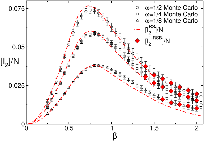
Figure 10: The classical mutual information per spin $[{\mathcal{I}}_{2}]/N$ in the S-K model on the $2$-sheets booklet: $[{\mathcal{I}}_{2}]/N$ plotted versus $\beta$. The symbols denote the Monte Carlo results extrapolated to the thermodynamic limit for booklet ratios $\omega=1/2,1/4,1/8$ (circles, squares, triangles). The dash-dotted lines are the analytical results in the replica-symmetric (RS) approximation. The full symbols (rhombi) are the results in the first-step replica-symmetry-breaking (1-RSB) approximation.

We first discussed the thermodynamic phase diagram of the S-K model on the $n$-sheets booklet, as a function of temperature, and the aspect ratio $\omega$ (cf. Eq. (3)). For any fixed $\omega$ the S-K model exhibits a low-temperature glassy phase, which is divided by the standard paramagnetic one at high temperatures by a phase transition. The critical inverse temperature $\beta_{c}$ exhibits a non trivial decreasing behavior as a function of $\omega$. Moreover, one has $\beta_{c}=1$ and $\beta_{c}=1/2$ for $\omega=0$ and $\omega=1$, respectively. In the high-temperature region the permutation symmetry among both the replicas and the physical sheets is preserved. This allowed us to provide an exact analytic expression for the free energy of the model and several derived quantities, such as the internal energy. We compared our results with Monte Carlo simulations, finding perfect agreement. Oppositely, in the low-temperature phase the replica symmetry is broken. For instance, we numerically observed that the replica-symmetric (RS) result for the internal energy is systematically lower than the Monte Carlo data, as in the standard S-K model sherrington-1978-prl ; sherrington-1978 . This discrepancy becomes larger upon lowering the temperature.

Inspired by the Parisi scheme parisi-1979 , we devised a systematic way of breaking the replica symmetry in successive steps. Our scheme breaks only the symmetry among the fictitious replicas, preserving that among the physical ones. Although this appears natural, we were not able to provide a rigorous proof that this is the correct symmetry breaking pattern. As a consequence, our scheme should be regarded as an approximation, and not as an exact solution. Moreover, we restricted ourselves to the one-level replica symmetry breaking ($1$-RSB). Surprisingly, the $1$-RSB result for the internal energy are in excellent agreement with the Monte Carlo data for $\beta\lesssim 3$, whereas the RS approximation fails already at $\beta\approx 1$. This suggests that the $1$-RSB ansatz captures correctly some aspects of the replica symmetry breaking.

Clear signatures of the replica symmetry breaking can be observed in the behavior of $[S_{2}]$. First, since $[S_{2}]$ exhibits the volume law behavior $[S_{2}]\propto N$, we considered its density $[S_{2}]/N$. For finite-size systems, and for any $\omega$, $[S_{2}]/N$ exhibits a maximum at infinite temperature, and it is a decreasing function of the temperature, as expected. Finite-size corrections are negligible at high temperatures, whereas they increase upon lowering the temperature. In the paramagnetic phase we were able to determine the functional form of $[S_{2}]/N$ in the thermodynamic limit, using the replica-symmetric approximation. This perfectly matched the Monte Carlo data. At low temperatures deviations from the RS result are present, reflecting the replica symmetry breaking. Remarkably, the one-step replica symmetry breaking ($1$-RSB) result $[S_{2}^{1\textrm{-}RSB}]/N$ fully describes the Monte Carlo data for $\beta\lesssim 3$, consistent with what was observed for the internal energy.

Finally, we considered the Rényi mutual information $[{\mathcal{I}}_{2}]$. This obeys a volume law for any $\beta$ and $\omega$, in contrast with local spin models, where an area law is observed wolf-2008 . The corresponding density $[{\mathcal{I}}_{2}]/N$ vanishes in both the infinite-temperature and the zero-temperature limits. Surprisingly, $[{\mathcal{I}}_{2}]/N$ does not exhibit any crossing for different system sizes at the paramagnetic-glassy transition, in striking contrast with local spin models jaconis-2013 . For any $\omega$, $[{\mathcal{I}}_{2}]/N$ exhibits a maximum for $\beta\approx 1$. The position of this maximum is not simply related to the paramagnetic-glassy transition. At high temperature $[{\mathcal{I}}_{2}]/N$ is described analytically by the RS result $[{\mathcal{I}}_{2}]^{RS}/N$. Deviations from the RS result, if present, are $\lesssim 10^{-3}$. On the other hand, at low temperatures one has to include the effects of the replica symmetry breaking. Similar to $[S_{2}]$, the $1$-RSB approximation $[{\mathcal{I}}^{1\textrm{-}RSB}_{2}]/N$ is in good agreement with the Monte Carlo data for $\beta\lesssim 3$.

Our work opens several research directions. First, it would be interesting to extend our results taking into account the full breaking of the replica symmetry, i.e., going beyond the one-step replica symmetry breaking approximation. This would allow us to reach a conclusion on the correctness of the replica symmetry breaking scheme that we used. Moreover, it would be interesting to discuss the finite size-corrections to the saddle point approximation. An intriguing direction would be to investigate whether the glassy critical behavior is reflected in the volume-law corrections to the classical Rényi entropies and mutual information. Finally, it would be interesting to extend our results to quantum spin systems exhibiting glassy behavior and replica symmetry breaking read-1995 ; andreanov-2012 .

X Acknowledgements

We would like to thank Pasquale Calabrese for useful discussions. V.A. acknowledges financial support from the ERC under Starting Grant 279391 EDEQS. S.I. and L.P. acknowledge support from the FP7/ERC Starting Grant No. 306897.

Appendix A The saddle point equations

In this section we provide the analytical expression for the saddle point equations (22)(23), which determine the overlap tensor $q_{\gamma\gamma^{\prime}}^{rr^{\prime}}$ (see section III.2). We restrict ourselves to zero magnetic field and to the $2$-sheets booklet (see Fig. 1). It is straightforward to generalize the calculation to the case with non zero magnetic field and to the $n$-sheets booklet. Here we provide the saddle point equations for both the replica-symmetric (RS) (see section IV.3) and the one-step replica symmetry breaking ($1$-RSB) approximations (see section V).

A.1 The replica-symmetric (RS) approximation

In the replica-symmetric approximation $q_{\gamma\gamma^{\prime}}^{rr^{\prime}}$ depends on the two parameters $q_{0},q_{0}^{\prime}\in\mathbb{R}$ (cf. Eq. (37)). The saddle point equations are derived from the RS approximation for the free energy $[F_{RS}(\omega,n,\beta)]$ (cf. Eq. (38)) as $\nabla_{\mathbf{q}}[F_{RS}(\omega,2,\beta)]=0$, where $\mathbf{q}\equiv(q_{0},q_{0}^{\prime})$, and $\nabla_{\mathbf{q}}\equiv\partial/\partial\mathbf{q}$. A straightforward calculation gives

$$\frac{1-q_{0}}{1-\omega}=2\int dzG_{0}(z)(1+\exp(2\beta^{2}(q_{0}-q_{0}^{\prime}))\cosh(2z))^{-1},$$ (58)

and

$$2\beta^{2}\frac{1-q_{0}^{\prime}}{1-\omega}=\int dzG_{0}(z)\Big{\{}\frac{\omega}{1-\omega}\Delta_{0}(z)\log\cosh(2z)\\ +\Delta_{0}(z)\log(1+\exp(2\beta^{2}(q_{0}-q_{0}^{\prime}))\cosh(2z))\\ +2\beta^{2}(1+\exp(2\beta^{2}(q_{0}-q_{0}^{\prime}))\cosh(2z))^{-1}\Big{\}},$$ (59)

where we defined $\Delta_{0}(z)$ as

$$\Delta_{0}(z)\equiv\frac{z^{2}}{2\beta^{2}q_{0}^{\prime 2}}-\frac{1}{2q_{0}^{\prime}},$$ (60)

and the so-called heat kernel $G_{0}(z)$ as

$$G_{0}(z)\equiv\frac{1}{\sqrt{2\pi\beta^{2}q_{0}^{\prime}}}\exp\Big{(}-\frac{z^{2}}{2\beta^{2}q_{0}^{\prime}}\Big{)}.$$ (61)

Notice that $\int dzG_{0}(z)\Delta_{0}(z)=0$.

A.2 The one-step replica symmetry breaking ($1$-RSB) approximation

In the one-step replica symmetry breaking approximation (see section V) $q_{\gamma\gamma^{\prime}}^{rr^{\prime}}$ depends on the four parameters $q_{0},q_{0}^{\prime},q_{1}^{\prime},m_{1}\in\mathbb{R}$. The saddle point equations are given as $\nabla_{\mathbf{p}}[F_{1\textrm{-}RSB}]=0$, where $\mathbf{p}\equiv(q_{0},q_{0}^{\prime},q_{1}^{\prime},m_{1})$, and $[F_{1\textrm{-}RSB}]$ is the disorder-averaged free energy given in Eq. (49). It is useful to define the modified heat kernel $G_{1}(z)$ as

$$G_{1}(z)\equiv\frac{1}{\sqrt{2\pi\beta^{2}(q_{1}^{\prime}-q_{0}^{\prime})}}\exp\Big{(}-\frac{z^{2}}{2\beta^{2}(q_{1}^{\prime}-q_{0}^{\prime})}\Big{)},$$ (62)

and

$$\Delta_{1}(z)\equiv\frac{z^{2}}{\beta^{2}(q_{1}^{\prime}-q_{0}^{\prime})^{2}}-\frac{1}{q_{1}^{\prime}-q_{0}^{\prime}}$$ (63)

$$\Gamma(z)\equiv\Big{\{}\int dz^{\prime}G_{1}(z^{\prime})\cosh^{m_{1}}(2z+2z^{\prime})\Big{\}}^{-1}$$

$$\Gamma^{\prime}(z)\equiv\Big{\{}\int dz^{\prime}G_{1}(z^{\prime})\Big{(}1+\cosh(2z+2z^{\prime})\Big{)}^{m_{1}}\Big{\}}^{-1}$$

$$\Theta(z,z^{\prime})\equiv 1+\exp(2\beta^{2}(q_{0}-q_{1}^{\prime}))\cosh(2z+2z^{\prime}).$$

Finally, the saddle point equations for $q_{0},q_{0}^{\prime},q_{1}^{\prime},m_{1}$ are obtained as

$$0=(1+q_{0}-2\omega)\exp(-2\beta^{2}(q_{0}-q_{1}^{\prime}))-2(1-\omega)\int dzdz^{\prime}G_{0}(z)\Gamma^{\prime}(z)G_{1}(z^{\prime})\cosh(2z+2z^{\prime})\Theta^{m_{1}-1}(z,z^{\prime})$$ (64)

$$0=4\beta^{2}m_{1}q_{0}^{\prime}+\frac{\omega}{m_{1}}\int dzG_{0}(z)\Delta_{0}(z)\log\int dz^{\prime}G_{1}(z^{\prime})\cosh^{m_{1}}(2z+2z^{\prime})\\ +\frac{1-\omega}{m_{1}}\int dzG_{0}(z)\Delta(z)\log\int dz^{\prime}G_{1}(z^{\prime})\Theta^{m_{1}}(z,z^{\prime})-\frac{\omega}{m_{1}}\int dzdz^{\prime}G_{0}(z)\Gamma(z)G_{1}(z^{\prime})\Delta_{1}(z^{\prime})\cosh^{m_{1}}(2z+2z^{\prime})\\ -\frac{1-\omega}{m_{1}}\int dzdz^{\prime}G_{0}(z)\Gamma^{\prime}(z)G_{1}(z^{\prime})\Delta_{1}(z^{\prime})\Theta^{m_{1}}(z,z^{\prime})$$ (65)

$$0=-4\beta^{2}(m_{1}-1)q_{1}^{\prime}-4\beta^{2}\omega+\frac{\omega}{m_{1}}\int dzdz^{\prime}G_{0}(z)\Gamma(z)G_{1}(z^{\prime})\Delta_{1}(z^{\prime})\cosh^{m_{1}}(2z+2z^{\prime})\\ +\frac{1-\omega}{m_{1}}\int dzdz^{\prime}G_{0}(z)\Gamma^{\prime}(z)G_{1}(z^{\prime})\Big{\{}\Delta_{1}(z^{\prime})\Theta^{m_{1}}(z,z^{\prime})-4\beta^{2}m_{1}\exp(2\beta^{2}(q_{0}-q_{1}^{\prime}))\cosh(2z+2z^{\prime})\Theta^{m_{1}-1}(z,z^{\prime})\Big{\}}$$ (66)

$$0=-\beta^{2}(q_{1}^{\prime 2}-q_{0}^{\prime 2})+\frac{\omega}{m_{1}}\int dzdz^{\prime}G_{0}(z)\Gamma(z)G_{1}(z^{\prime})\cosh^{m_{1}}(2z+2z^{\prime})\log\cosh(2z+2z^{\prime})\\ +\frac{1-\omega}{m_{1}}\int dzdz^{\prime}G_{0}(z)\Gamma^{\prime}(z)G_{1}(z^{\prime})\Theta^{m_{1}}(z,z^{\prime})\log(\Theta(z,z^{\prime}))-\frac{1-\omega}{m_{1}^{2}}\int dzG_{0}(z)\log\int dz^{\prime}G_{1}(z^{\prime})\Theta^{m_{1}}(z,z^{\prime})\\ -\frac{\omega}{m_{1}^{2}}\int dzG_{0}(z)\log\int dz^{\prime}G_{1}(z^{\prime})\cosh^{m_{1}}(2z+2z^{\prime}).$$ (67)

Appendix B Mutual information in the infinite-range clean Ising model

Here we discuss the Rényi entropy $S_{2}$ and the associated mutual information ${\mathcal{I}}_{2}$ in the infinite-range Ising model without disorder, defined by the hamiltonian

$${\mathcal{H}}=-\frac{J}{N}\sum\limits_{i<j}S_{i}S_{j}+h\sum_{i}S_{i}.$$ (68)

We consider the situation without external magnetic field, i.e., $h=0$ and fix $J=1$. The phase diagram of the model exhibits a paramagnetic phase at high temperature, while at low temperatures there is ferromagnetic order. The two phases are separated by a phase transition at $\beta_{c}=1$. We consider both the situations with finite $N$ as well as the thermodynamic limit. For finite $N$ we provide exact numerical results for $S_{2}$ and ${\mathcal{I}}_{2}$, while we address the thermodynamic limit using the booklet construction (see II) and the saddle point approximation.

Similar to the S-K model, we find that the para-ferro transition persists on the booklet, and the critical temperature depends on the booklet ratio $\omega$. The Rényi entropy $S_{2}$ and the mutual information ${\mathcal{I}}_{2}$ are extensive, and their densities $S_{2}/N,{\mathcal{I}}_{2}/N$ finite and smooth at any temperature. Notice that this different for the Shannon mutual information wilms-2012 ${\mathcal{I}}_{1}$, which is finite (i.e., ${\mathcal{I}}_{1}\sim{\mathcal{O}}(1)$) in the whole phase diagram, except for a logarithmically divergent behavior (with system size) at the critical point $\beta_{c}=1$.

Finally, we show that the information about the phase transition is encoded in the subleading, i.e. $o(N)$, corrections of ${\mathcal{I}}_{2}$. Precisely, logarithmically divergent contributions are present at $\beta=1/2,1$ and $\beta=\beta_{c}(\omega)$, with $\beta_{c}(\omega)$ the critical temperature of the model on the booklet at fixed aspect ratio $\omega$.

B.1 Saddle point approximation

We first discuss the thermodynamic limit. The calculation of the booklet partition function $Z(\omega,n,\beta)$ (see section II) can be done using the same techniques as in section III. The result reads

$$Z(\omega,n,\beta)=\exp\Big{(}-\frac{\beta}{2}n\Big{)}\Big{(}2\pi\frac{\beta}{N}\Big{)}^{-\frac{n}{2}}\int\prod_{\delta}dz_{\delta}\exp N\Big{\{}\\ -\sum_{\delta}\Big{[}\frac{z^{2}_{\delta}}{2\beta}-(1-\omega)\log(2\cosh z_{\delta})\Big{]}+\omega\log(2\cosh\sum_{\delta}z_{\delta})\Big{\}},$$ (69)

with $\delta=1,\dots,n$. Using the saddle point approximation, from (69) one obtains $F(\omega,n,\beta)\equiv\log Z(\omega,n,\beta)$ as

$$F(\omega,n,\beta)\approx N\Big{\{}-\sum_{\delta}\Big{[}\frac{z^{2}_{\delta}}{2\beta}-(1-\omega)\log(2\cosh z_{\delta})\Big{]}\\ +\omega\log(2\cosh\sum_{\delta}z_{\delta})\Big{\}},$$ (70)

where we neglected subleading contributions $o(N)$. The parameters $\{z_{\delta}\}_{\delta=1}^{n}$ are solutions of the saddle point equations

$$0=z_{\delta}-\beta(1-\omega)\tanh z_{\delta}-\beta\omega\tanh\big{(}\sum_{\delta}z_{\delta}\big{)},\quad\forall\delta.$$ (71)

For $n=2$, the system (71) becomes

$$0=z_{1}-\beta(1-\omega)\tanh z_{1}-\beta\omega\tanh\big{(}z_{1}+z_{2}\big{)}$$ (72)

$$0=z_{2}-\beta(1-\omega)\tanh z_{2}-\beta\omega\tanh\big{(}z_{1}+z_{2}\big{)}.$$ (73)

The system has the solutions $z_{1}=z_{2}=z_{s}=0$ for $\beta\leq\beta_{c}=1/(1+\omega)$, and $z_{1}=z_{2}=z_{s}\neq 0$ for $\beta>\beta_{c}$. Note that $\beta_{c}$ is different in presence of disorder (see (44)).

The solution $z_{s}$ of the saddle point equations (71) is shown in Fig. 11 as a function of $\beta$ for $\omega=0,1/2,1$. The vertical-dotted line is $\beta_{c}$ for $\omega=1/2$. Notice that at low temperatures $z_{s}$ is independent on $\omega$, and one has $z_{s}\sim\beta$.

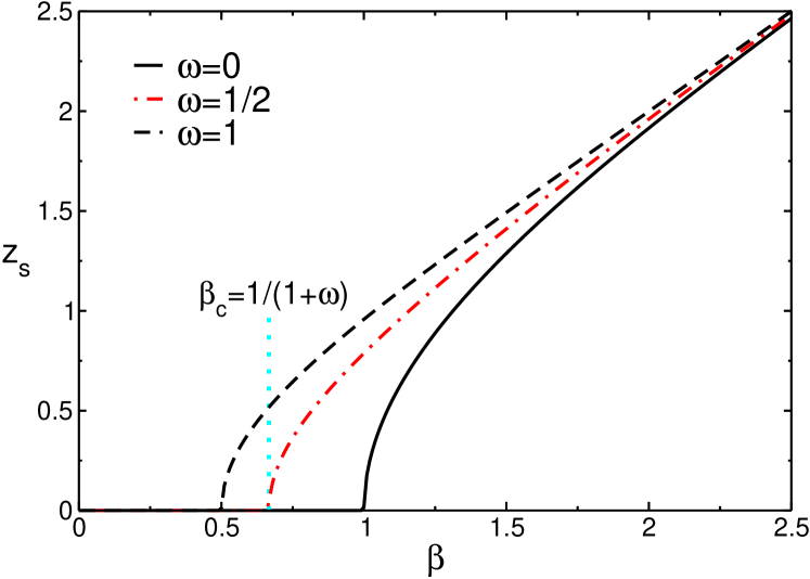
Figure 11: The infinite-range Ising model on the $2$-sheets booklet: saddle point approximation. The solution $z_{s}$ of the saddle point equations (71) plotted as a function of the inverse temperature $\beta$ and for booklet aspect ratio $\omega=0,1/2,1$. The vertical dotted line denotes the critical inverse temperature for $\omega=1/2$.

B.2 Rényi entropy and mutual information: saddle point results

It is straightforward to obtain the Rényi entropies $S_{n}=(F(\omega=0,n,\beta)-F(\omega,n,\beta))/(n-1)$ using (70) and (5). Figure 12 plots the entropy density $S_{2}/N$ versus the inverse temperature $\beta$. $S_{2}$ exhibits a volume-law behavior $S_{2}\propto N$ for all values of $\beta$ and $\omega$. The different curves correspond to different booklet aspect ratios $\omega$. For $\beta\leq\beta_{c}$ one has the flat behavior $S_{2}=\omega\log(2)$, whereas $S_{2}$ is vanishing in the low-temperature regime. The full symbol (rhombi) in Figure 12 are exact results for a booklet with $N=400$ spins per sheet (see next section), and are in good agreement with the saddle point approximation results.

The mutual information per spin ${\mathcal{I}}_{2}/N$ is reported in Figure 13. The lines are the analytical results for booklet aspect ratios $\omega=1/20,1/4,1/2$, while the full symbols are the exact results for the booklet with $N=400$ spins per sheet. Clearly, ${\mathcal{I}}_{2}/N$ is exactly zero in the high-temperature region for $\beta\leq 1/2$, it exhibits at maximum at $\beta\approx 1$, and it is vanishing in the limit $\beta\to\infty$.

Finally, one should stress that a dramatically different behavior is observed in the Shannon mutual information ${\mathcal{I}}_{1}\equiv\lim_{n\to 1}{\mathcal{I}}_{n}$. Specifically, ${\mathcal{I}}_{1}$ is finite in the thermodynamic limit, and it only exhibits a logarithmic divergence as ${\mathcal{I}}=1/4\log(N)$ at the critical point $\beta_{c}=1$ (see Ref. wilms-2012, ).

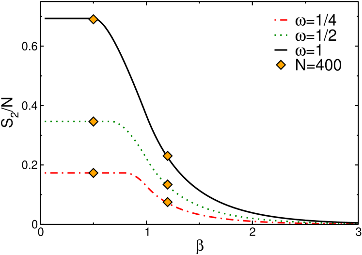
Figure 12: The infinite-range Ising model on the $2$-sheets booklet in the thermodynamic limit: the classical Rényi entropy density $S_{2}/N$, with $N$ the total number of spins on a single sheet of the booklet. $S_{2}/N$ is plotted against the inverse temperature $\beta$ and for booklet aspect ratio $\omega=1/4,1/2,1$. Note tht at high temperature $S_{2}=\omega\log(2)$. The lines are obtained using the saddle point approximation, while the full symbols denote the exact numerical results for a finite system with $N=400$.

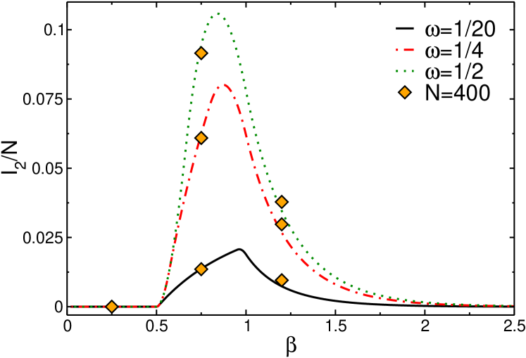
Figure 13: The infinite-range Ising model on the $2$-sheets booklet in the thermodynamic limit: the classical mutual information density ${\mathcal{I}}_{2}/N$ plotted against the inverse temperature $\beta$ and for booklet aspect ratio $\omega=1/4,1/2,1$. Note that ${\mathcal{I}}_{2}=0$ for $\beta\leq 1/2$. The full symbols are the the exact numerical results for a finite system with $N=400$.

B.3 Rényi entropy and mutual information: Exact treatment

For finite $N$, $S_{2}$ and ${\mathcal{I}}_{2}$ can be calculated exactly using the results obtained in Ref. wilms-2012, . The eigenstates of (68) are product states. They can be characterized as $|p,i\rangle$, with $p$ the total number of up spins (the remaining $N-p$ being down spins) and $i$ labelling the $B(N,p)\equiv N!/(p!(N-p)!)$ eigenstates with the same $p$. The partition function of (68) is given as

$$Z(\beta)\equiv\textrm{Tr}\rho=\sum\limits_{p=0}^{N}B(N,p)e^{2N\beta(\frac{p}{N}-\frac{1}{2})^{2}}.$$ (74)

Similarly, one has

$$Z^{n}(\beta)\equiv\textrm{Tr}\sum\limits_{p=0}^{N}B(N,p)e^{2nN\beta(\frac{p}{N}-\frac{1}{2})^{2}}.$$ (75)

The thermal density matrix $\rho$ is defined as $\rho\equiv 1/Ze^{-\beta{\mathcal{H}}}$. Given a bipartition of the spins into two groups $A$ and $B$ containing $N_{A}$ and $N-N_{A}$ spins, respectively, the reduced density matrix for $A$ is obtained as wilms-2012

$$\rho_{A}\equiv\frac{1}{Z}\textrm{Tr}_{B}\sum\limits_{p,i}e^{2N\beta(\frac{p}{N}-\frac{1}{2})^{2}}|p,i\rangle\langle p,i|.$$ (76)

By performing the trace over part $B$ one obtains

$$\rho_{A}=\sum\limits_{p_{A},i_{A}}R(p_{A})|p_{A},i_{A}\rangle\langle p_{A},i_{A}|,$$ (77)

where $|p_{A},i_{A}\rangle$ form a basis for part $A$ of the system and

$$R(p_{A})\equiv\frac{1}{Z}\sum\limits_{p_{B}=0}^{N-N_{A}}B(N-N_{A},p_{B})e^{2N\beta(\frac{p_{A}}{N}+\frac{p_{B}}{N}-\frac{1}{2})^{2}}.$$ (78)

From (77) it is straightforward to obtain

$$\textrm{Tr}\rho_{A}^{n}=\sum\limits_{p_{A}=0}^{N_{A}}B(N_{A},p_{A})R^{n}(p_{A}).$$ (79)

Similarly, $\textrm{Tr}\rho^{n}_{B}$ is obtained from (79) substituting $A\to B$ and $N_{A}\to N-N_{A}$, while $\textrm{Tr}\rho^{n}_{A\cup B}\equiv\textrm{Tr}\rho^{n}$. The Rényi entropies $S_{n}$ and the mutual informations ${\mathcal{I}}_{n}$ can be calculated numerically using (79), (75) and the definitions (2) (4). The numerical results for $S_{2}$ and ${\mathcal{I}}_{2}$ for a system with $N=400$ spins are shown in Figure 12 and Figure 13, and are in good agreement with the results in the thermodynamic limit.

Figure 14 focuses on the finite-size subextensive corrections for ${\mathcal{I}}_{2}$. We plot ${\mathcal{I}}_{2}-{\mathcal{I}}^{(sp)}_{2}$, with ${\mathcal{I}}_{2}^{(sp)}$ denoting the saddle point extensive part of ${\mathcal{I}}_{2}$. We restrict ourselves to $\omega=N_{A}/N=1/2$, although similar results have to be expected at different $\omega$. Clearly, ${\mathcal{I}}_{2}-{\mathcal{I}}_{2}^{(sp)}$ is vanishing at high temperatures, whereas one has ${\mathcal{I}}_{2}-{\mathcal{I}}_{2}^{(sp)}\to\log(2)$ in the limit $\beta\to\infty$ (horizontal line). Surprisingly, ${\mathcal{I}}_{2}-{\mathcal{I}}_{2}^{(sp)}$ diverges in the thermodynamic limit for $\beta=1/2,2/3,1$ (vertical lines in the Figure), which are the critical temperatures for the model on a booklet with $\omega=1,1/2,0$. This divergence is logarithmic as a function of $N$, as confirmed in Figure 15 plotting $|{\mathcal{I}}_{2}-{\mathcal{I}}_{2}^{(sp)}|$ versus $\log(N)$ for fixed $\beta=1/2,2/3,1$. Interestingly, the precise behavior depends on $\beta$. One has $|{\mathcal{I}}_{2}-{\mathcal{I}}_{2}^{(sp)}|\propto 1/4\log(N)$ for $\beta=1/2$ and $|{\mathcal{I}}_{2}-{\mathcal{I}}_{2}^{(sp)}|\propto 1/2\log(N)$ for $\beta=2/3$ and $\beta=1$. Again, this is dramatically different for the von Neumann mutual information ${\mathcal{I}}_{1}=\lim_{n\to 1}{\mathcal{I}}_{n}$, which exhibits only one divergent peak wilms-2012 at $\beta=1$.

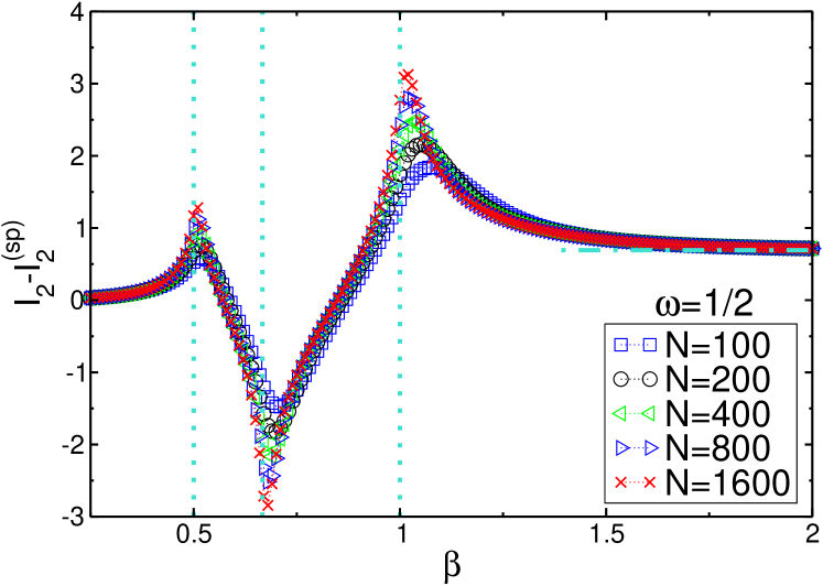
Figure 14: The infinite-range Ising model on the $2$-sheets booklet: saddle point corrections. The correction for the mutual information ${\mathcal{I}}_{2}-{\mathcal{I}}_{2}^{(sp)}$ are plotted against the inverse temperature $\beta$. The data are for a booklet with aspect ratio $\omega=1/2$. Here ${\mathcal{I}}_{2}^{(sp)}$ are the same data as in Figure 13 (dotted line). The vertical lines denote the critical temperatures $\beta_{c}$ for $\omega=1,1/2,0$ (from left to right). The horizontal dash-dotted line is $\log(2)$. Note the (logarithmically) divergent behavior at $\beta_{c}$.

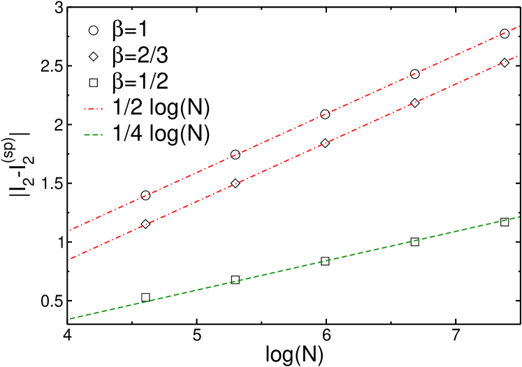
Figure 15: The infinite-range Ising model on the $2$-sheets booklet: Scaling of the corrections of the mutual information ${\mathcal{I}}_{2}$ at the booklet critical points $\beta_{c}=1/2,2/3,1$ (see vertical lines in Figure 14). We plot $|{\mathcal{I}}_{2}-{\mathcal{I}}_{2}^{(sp)}|$ versus $\log(N)$, with $N$ the number of spins on one sheet of the booklet. Here ${\mathcal{I}}_{2}^{(sp)}$ is the same as in Figure 13 (dotted line).

Appendix C Monte Carlo method to calculate the classical Rényi entropies

Here we describe the Monte Carlo method that we used to calculate the Rényi entropies $S_{n}$ and the mutual information ${\mathcal{I}}_{n}$. The method exploits the representation of $S_{n}$ as ratio of partition functions as

$$S_{n}(A)\equiv\frac{1}{1-n}\log\left(\frac{Z(A,n,\beta)}{Z^{n}(\beta)}\right),$$ (80)

where $Z(A,n,\beta)$ and $Z(\beta)$ are the partition functions of the model on the booklet and on the plane, respectively (see Fig. 1 and section II for the definitions). There are only few approaches to numerically calculate the ratio of partition functions in Eq. (80). For instance, a brute force numerical integration of the internal energy as a function of temperaturejaconis-2013 can be used to calculate $Z(A,n,\beta)$ and $Z(\beta)$. However, this requires high accuracy over a large range of temperature.

Here we directly measure the ratio of partition functions using the so-called ratio trick. In the ratio trick one splits the subsystem $A$ in a set of subsystems $A_{i}$ such that $A_{i}\subset A_{i+1}$, and the largest subsystem in the set is simply $A$ itself. Then one writes

$$\frac{Z(A,n,\beta)}{Z^{n}(\beta)}=\prod_{i=0}^{N/4-1}\frac{Z(A_{i},n,\beta)}{Z(A_{i+1},n,\beta)},$$ (81)

where for simplicity we specialized to intervals $A_{i}$ such that

$$A_{i}=4i,\quad i\in[0,N/4].$$ (82)

Crucially, if the length of $A_{i}$ increases mildly with $i$, each term in the product in the right-hand side of Eq. (81) can be sampled efficiently in Monte Carlo stephan-2014 . Notice that the same trick has also been used in Ref. alba-2010, ; alba-2011, ; alba-2013, . More specifically, one can write

$$\frac{Z(A_{i},n,\beta)}{Z(A_{j},n,\beta)}=\frac{T_{j\rightarrow i}}{T_{i\rightarrow j}},$$ (83)

where $T_{i\rightarrow j}$ is the (Monte Carlo) transition probability from a spin configuration living on the booklet with subregion $A=A_{i}$ to a spin configuration living on the booklet with $A=A_{j}$. Notice that spins in region $A$ of different sheets are identified (cf. Eq. (8)). Clearly, if $j<i$ one has $T_{i\rightarrow j}=1$. When $j>i$ a naive method to determine $T_{i\rightarrow j}$ would be to simply count the fraction of times (during the Monte Carlo update) that a spin configuration living on the booklet with $A=A_{i}$ is also a valid spin configuration on the booklet with $A=A_{j}$. In the following we provide a more efficient scheme to calculate $T_{i\rightarrow j}$. To summarize, our approach for calculating the ratio of partition functions in Eq. (81) consists of four steps:

1. Do a full Monte Carlo sweep of the system on the booklet with $A=A_{i}$ to generate an importance sampled spin configuration. This can be done with any update scheme, such as standard Metropolis or cluster updates.

2. For the spins living in the set difference $A_{i+1}\setminus A_{i}$ calculate

   $$W_{a}=\prod_{n}\sum_{i_{n}}e^{-\beta E_{i_{n}}}.$$ (84)

   Here (cf. Eq. (82)) $i$ runs over all the $2^{4}$ configurations of the four spins in $A_{i+1}\setminus A_{i}$ for each of the $n$ sheets, and $E_{i_{n}}$ is the energy associated with the spin configuration $i_{n}$ on a single sheet.

3. Calculate the quantity

   $$W_{b}=\sum_{j}e^{-\beta E_{j}}.$$ (85)

   As in step $2$, $j$ runs over all the $2^{4}$ configurations of the four spins living in $A_{i+1}\setminus A_{i}$, but since the spins living on different sheets are identified there are only $2^{4}$ configurations in total and the energy $E_{i}$ is that of all $n$ sheets together.

4. Calculate the transition probability $T_{i\rightarrow i+1}$ as

   $$T_{i\rightarrow i+1}=\Bigl{<}\frac{W_{b}}{W_{a}}\Bigr{>},$$ (86)

where the angular brackets denote the Monte Carlo average. This method is much faster than simply counting configurations as it allows us to integrate over all possible configurations of the spins in $A_{i+1}\setminus A_{i}$, treating the remaining ones as a bath that is updated by the regular Monte Carlo update. The computational cost of this procedure grows exponentially with the number of spins in $A_{i+1}\setminus A_{i}$. In our Monte Carlo simulations we calculate $Z(A_{i},n,\beta)/Z(A_{i+1},n,\beta)$ for every disorder realization and $S_{n}(A)$ using Eq. (80). Finally, we average over the disorder to obtain $[S_{n}(A)]$.

References

- (1) K. Binder and A. P. Young, Rev. Mod. Phys. 58, 801 (1986).
- (2) M. Mezard, G. Parisi, and M. Virasoro, Spin Glass theory and beyond, World Scientific, Singapore (1987).
- (3) A. P. Young, Spin Glasses and Random Fields (Singapore: World Scientific).
- (4) H. Nishimori, Statistical Physics of Spin Glasses and Information Processing, Clarendon Press, Oxford (2001).
- (5) T. Castellani and A. Cavagna, J. Stat. Mech. (2005) P05012.
- (6) D. Sherrington and S. Kirkpatrick, Phys. Rev. B 17, 4385 (1978).
- (7) D. Sherrington and S. Kirkpatrick, Phys. Rev. Lett. 35, 1972 (1978).
- (8) G. Parisi, J. Phys. A 13, 1101 (1980).
- (9) M. Talagrand, Ann. of Math. 163, 221 (2006).
- (10) L. A. Pastur and M. V. Shcherbina, J. Stat. Phys. 62, 1 (1991).
- (11) M. Mezard, G. Parisi, N. Sourlas, G. Toulouse, and M. Virasoro, Phys. Rev. Lett. 52, 1156 (1984).
- (12) R. Rammal, G. Toulouse, and M. A. Virasoro, Rev. Mod. Phys. 58, 765 (1986).
- (13) J. Cardy, Scaling and Renormalization in Statistical Physics (Cambridge Lecture Notes in Physics).
- (14) B. Yucesoy, H. G. Katzgraber, and J. Machta, Phys. Rev. Lett. 109, 177204 (2012).
- (15) A. Billoire, L. A. Fernandez, A. Maiorano, E. Marinari, V. Martin-Mayor, G. Parisi, F. Ricci-Tersenghi, J. J. Ruiz-Lorenzo, and D. Yllanes, Phys. Rev. Lett. 110, 219701 (2013).
- (16) B. Yucesoy, H. G. Katzgraber, and J. Machta, Phys. Rev. Lett. 110, 219702 (2013)
- (17) S. Morrison, A. Kantian, A. J. Daley, H. G. Katzgraber, M. Lewenstein, H. P. Büchler, and P. Zoller, New J. Phys. 10, 073032 (2008).
- (18) P. Rotondo, E. Tesio, and S. Caracciolo, Phys. Rev. B 91, 014415 (2015).
- (19) N. Ghofraniha, I. Viola, F. Di Maria, G. Barbarella, G. Gigli, L. Leuzzi, and C. Conti, Nature Comm. 6, 6058 (2015).
- (20) L. Amico, R. Fazio, A. Osterloh, and V. Vedral, Rev. Mod. Phys. 80, 517 (2008).
- (21) J. Eisert, M. Cramer, and M. B. Plenio, Rev. Mod. Phys. 82, 277 (2009).
- (22) P. Calabrese, J. Cardy, and B. Doyon Eds., Special issue: Entanglement entropy in extended systems, J. Phys. A 42, 50 (2009).
- (23) P. Calabrese and J. Cardy, J. Phys. A 42 504005 (2009).
- (24) C. Holzhey, F. Larsen, and F. Wilczek, Nucl. Phys. B 424, 443 (1994).
- (25) G. Vidal, J. I. Latorre, E. Rico, and A. Kitaev, Phys. Rev. Lett. 90, 227902 (2003). J. I. Latorre, E. Rico, and G. Vidal, Quant. Inf. and Comp. 4, 048 (2004).
- (26) P. Calabrese and J. Cardy, J. Stat. Mech. (2004) P06002. P. Calabrese and J. Cardy, Int. J. Quant. Inf. 4, 429 (2006).
- (27) P. Calabrese, J. Cardy, and E. Tonni, Phys. Rev. Lett. 109, 130502 (2012).
- (28) J. Iaconis, S. Inglis, A. B. Kallin, and R. G. Melko, Phys. Rev. B 87, 195134 (2013).
- (29) J.-M. Stéphan, S. Inglis, P. Fendley, and R. G. Melko, Phys. Rev. Lett. 112, 127204 (2014).
- (30) F. C. Alcaraz and M. A. Rajabpour, Phys. Rev. Lett. 111, 017201 (2013).
- (31) J.-M. Stéphan, Phys. Rev. B 90, 045424 (2014).
- (32) M. M. Wolf, F. Verstraete, M. B. Hastings, and J. I. Cirac, Phys. Rev. Lett. 100, 070502 (2008).
- (33) G. Refael and J. E. Moore J. Phys. A: Math. Theor. 42 504010 (2009).
- (34) C. Castelnovo, C. Chamon, and D. Sherrington, Phys. Rev. B 81, 184303 (2010).
- (35) F. Guerra and F. L. Toninelli, Commun. Math. Phys. 230, 71 (2002).
- (36) E. Fradkin and J. E. Moore, Phys. Rev. Lett. 97, 050404 (2006).
- (37) E. Fradkin, J. Phys. A 42, 504011 (2009).
- (38) B. Hsu, M. Mulligan, E. Fradkin, and E.-A. Kim, Phys. Rev. B 79, 115421 (2009).
- (39) J-M Stéphan, S. Furukawa, G. Misguich, and V. Pasquier, Phys. Rev. B 80, 184421 (2009).
- (40) B. Hsu and E. Fradkin, J. Stat. Mech. (2010) P09004.
- (41) M. Oshikawa, arXiv:1007.3739 (2010).
- (42) J-M Stéphan, G. Misguich, and V. Pasquier, Phys. Rev. B, 82, 125455 (2010);
- (43) M. P. Zaletel, J. H. Bardarson, and J. E. Moore, Phys. Rev. Lett. 107, 020402 (2011).
- (44) J. R. L. de Almeida and D. J. Thouless, J. Phys. A 11, 983 (1978).
- (45) G. Parisi, Phys. Rev. Lett. 43, 1754 (1979).
- (46) J. Wilms, J. Vidal, F. Verstraete, and S. Dusuel, J. Stat. Mech. (2012) P01023.
- (47) G. Parisi, Phys. Rev. Lett 50, 1946 (1983).
- (48) K. Hukushima and K. Nemoto, J. Phys. Soc. Jpn. 65, 1604 (1996).
- (49) A. Billoire, in Rugged Free Energy Landscape, Springer Lecture Notes in Physics, edited by W. Janke (Springer, Berlin-Heidelberg 2007.
- (50) T. Aspelmeier, A. Billoire, E. Marinari, and M. A. Moore, J. Phys. A: Math. Theor. 41 324008 (2008).
- (51) N. Read, S. Sachdev, and J. Ye, Phys. Rev. B 52, 384 (1995).
- (52) A. Andreanov and M. Müller, Phys. Rev. Lett. 109, 177201 (2012).
- (53) V. Alba, L. Tagliacozzo, and P. Calabrese, Phys. Rev. B 81, 060411(R) (2010).
- (54) V. Alba, L. Tagliacozzo, and P. Calabrese, J. Stat. Mech. (2011) P06012.
- (55) V. Alba, J. Stat. Mech. (2013) P05013.