Multiple shooting-Local Linearization method for the identification of dynamical systems

Abstract

The combination of the multiple shooting strategy with the generalized Gauss-Newton algorithm turns out in a recognized method for estimating parameters in ordinary differential equations (ODEs) from noisy discrete observations. A key issue for an efficient implementation of this method is the accurate integration of the ODE and the evaluation of the derivatives involved in the optimization algorithm. In this paper, we study the feasibility of the Local Linearization (LL) approach for the simultaneous numerical integration of the ODE and the evaluation of such derivatives. This integration approach results in a stable method for the accurate approximation of the derivatives with no more computational cost than the that involved in the integration of the ODE. The numerical simulations show that the proposed Multiple Shooting-Local Linearization method recovers the true parameters value under different scenarios of noisy data.

Key words and phrases. Multiple Shooting, Local Linear Approximation, nonlinear equations, parameter estimation, chaotic dynamics, generalized Gauss-Newton, line search algorithm

1 Introduction

Ordinary differential equations (ODEs) are extensively used for modeling the temporal evolution of complex dynamical systems in dissimilar fields such as physics, economy, ecology, biology, chemistry and social sciences [1]. Typically, these ODEs contain parameters that are associated to phenomenological factors that control the basic variables interplay of the models. However, the values of such parameters are usually unknown and must be determined in such a way that the models reproduce the observed experimental data at best. Despite a time series analysis of observed experimental data can determine useful quantities that characterize the system dynamics (e.g., Lyapunov exponents, attractor dimension), identifying the system structure and estimating the corresponding parameters would be a matter of greater practical value. Thus, an accurate estimation of the non observed states and models’s parameters is not only critical to reproduce and describe a given dynamic behavior but also to understand the underlying causes of the analyzed processes. This is of particular importance for ODEs describing chaotic dynamics, where the trajectories of interest are very sensitive to small perturbations of the parameters and initial values ([2], [3], [4], [5]). In this circumstance, a major challenge is to find a proper numerical integrator able to preserve the stability of the solutions in situations of parameter-dependent instabilities in such a way that allows an accurate estimation of these parameters from noisy chaotic observations.

Several strategies have been proposed for dealing with the parameter estimation problem in ODEs given a set of noisy observations. Among them, the so-called Initial Value approach is perhaps the most known. In this approach, the estimated parameters are those that minimize the least square errors resulting from fitting the numerical solution of the corresponding Initial Value problem to the given observation data. However, as it has been pointed out in [6], [7], [8], the estimators resulting from this approach are very sensitive to the initial guess of the parameters and usually turn out only local optimum solutions. A class of estimation methods that overcome this drawback was originally introduced in [6] and it is currently known as the Boundary Value approach (see, e.g., [7], [3], [9], [10]). This approach has two distinctive components: 1) the introduction of several multiple shooting nodes for solving the ODE as multiple Initial Value Problems (IVPs) in smaller subintervals, and 2) the solution of a constrained least squares problem in an augmented set of parameters. The main advantage of this multiple shooting strategy is that the whole observed data can be easily used to bring information about the true solution of the ODE [7]. Thus, the solution of the multiple IVP remains close to the true solution since the initial iteration of the optimization algorithm. In this way,  the influence of the poor initial parameter estimates is considerably reduced. Besides, the splitting of the integration interval into multiple subintervals limits the error propagation and allows parameter estimation even for chaotic systems ([2], [3]). Despite the introduction of additional variables seems to yield a more complicated estimation procedure, it is actually increasing computational efficiency and numerical stability of the estimation method [7], [3]. A third estimation strategy, called nonparametric, employs nonparametric functions to represent the unknown solutions of the ODEs (see,e.g., [11], [12], [13], [8], [14]). Typically, this class of estimators require two levels of optimization. The lower level approximates non parametric functions to the ODE trajectories conditional on the ODE parameters, while the upper optimization level does the estimation of the parameters of interest. Clearly, as compared to the previous two approaches, this procedure increases the computational burden of the parameters estimation process.

As remarked in [8], a common difficulty of all these estimation strategies is the numerical computation of the derivatives of the trajectories with respect to the parameters of the ODE. With this respect, three main approximations have been commonly employed. The simplest one, finite differences, also called external differentiation [6], [7] is not usually recommended due to the high computational cost required for achieving numerically stable derivatives (see further discussion in [10]). The second one, called internal differentiation, consists on differentiating the numerical integrator corresponding to the original differential equation [6], [7], [15]. In general, internal differentiation is a mechanism less computationally intensive than the external differentiation but, it might introduce also high computational cost in the case of implicit integrators or integrators defined trough some numerical derivatives. The third approach ([6], [7], [10]) consists on approximating the variational equations that describe the temporal evolution of the required derivatives, which must be integrated simultaneously to original equation. As in the second kind of approximation, this can be also computationally intensive for certain types of numerical schemes.

In this paper, we study the feasibility of the Local Linearization (LL) technique (see, e.g., [16], [17]) for the simultaneous numerical integration of the IVPs and the evaluation of the numerical derivatives that appear in the multiple shooting method. In previous works [18], [19], [20] this LL technique has been successfully applied for the parameter estimation of ODEs in the context of the Initial-Value approach. This has been possible thanks to the convenient trade-off between the numerical accuracy, stability and computational cost of the LL integrators and their capability of preserve a number of dynamical behaviors of the ODEs, which became relevant for the parameter estimation. In addition to this and following the ideas used in [21] for the computation of the Lyapunov Exponents, the LL technique can be used for the numerical integration of the variational equations associated to the derivative with respect to the parameters and initial conditions with no more computational cost than the that involved in the integration of the ODE. Therefore, the application of the LL technique for identification of ODEs in the framework of Boundary Value approach is also attractive.

The paper is organized as follows. In Section 2, the essentials on the Multiple Shooting strategy and the generalized Gauss-Newton algorithm are presented. Section 3 is focused in the link of the LL technique to the multiple shooting method. The resulting algorithm for the parameter estimation is summarized in this section as well. The performance of the Multiple Shooting-Local Linearization method is presented in Section 4 throughout three numerical examples. Finally, some discussion and conclusions are presented in the last two sections.

2 Multiple Shooting Method

Let us consider the $d$-dimensional ODE

$$\overset{.}{\mathbf{x}}=\mathbf{f}(t,\mathbf{x,p});\ t\in[t_{0},T]$$ (1)

depending on a $p$-dimensional vector $\mathbf{p}$ of parameters, where $\mathbf{f}:\mathbb{R}\times\mathbb{R}^{d}\times\mathbb{R}^{p}\rightarrow\mathbb{R}^{d}$ is a smooth function.

A typical estimation problem for ODEs consist of finding optimal values for the parameters $\mathbf{p}$ based on the observation of some values of the state variable $\mathbf{x}$ contaminated with noise (i.e., data points). That is, suppose that a number of $N$ observed data points $\mathbf{z}_{i}$ related to the state variables $\mathbf{x}$ and parameters $\mathbf{p}$ via the observation equation

$$\mathbf{z}_{i}=\mathbf{g}(t_{i}^{\ast},\mathbf{x}(t_{i}^{\ast}),\mathbf{p})+\epsilon_{i},$$ (2)

are given at the time instants $t_{i}^{\ast}\in[t_{0},T]$, $i=1,...,N$, where $\mathbf{g}:\mathbb{R}\times\mathbb{R}^{d}\times\mathbb{R}^{p}\rightarrow\mathbb{R}^{v}$ is a smooth function, and $\epsilon_{i}$ denotes the measurement errors. If the measurement errors are assumed independent, Gaussian distributed with zero mean and known variance $\sigma^{2}$, then the minimization of the weighted least-squares objective function

$$J(\mathbf{p})=\sum\limits_{i=1}^{N}\sum\limits_{j=1}^{v}\sigma^{-2}(\mathbf{z}_{i}^{j}-\mathbf{g}^{j}(t_{i}^{\ast},\mathbf{x}(t_{i}^{\ast},\mathbf{p}),\mathbf{p}))^{2}$$

with respect to $\mathbf{p}$ yields a maximum likelihood estimator for the parameters of the ODE (1).

2.1 Nonlinear optimization problem

Formally, the least squares problem described so far is a unconstrained optimization problem of the type

$$\min_{\mathbf{p}}\{\left\|\mathbf{F}_{1}(\mathbf{p})\right\|_{2}^{2}\},$$

where $\mathbf{F}_{1}(\mathbf{p})=vec(\mathbf{M}(\mathbf{p}))$ is a $Nv$-dimensional vector, $\mathbf{M}(\mathbf{p})$ is a $N\times v$ matrix with entries $\mathbf{M}^{ji}(\mathbf{p})$ $=$ $\sigma^{-1}(\mathbf{z}_{i}^{j}-\mathbf{g}^{j}(t_{i}^{\ast},\mathbf{x}(t_{i}^{\ast}),\mathbf{p}))$ for all $i=1,...,N$ and $\ j=1,...,v$, and $vec(.)$ denotes the vectorization operator.

However, in many applications, certain initial/boundary problems as those that appear in control engineering problems (see, e.g., [22]) additional requirements for the solutions and parameters must be satisfied. Mathematically, these restrictions are represented by a vector of (component wise) equality and/or inequality conditions of the form

$$\mathbf{R}(t_{1}^{\ast},\mathbf{x}(t_{1}^{\ast}),...,t_{N}^{\ast},\mathbf{x(}t_{N}^{\ast}\mathbf{)},\mathbf{p})=0\text{ or }\geq 0.$$

In this situation, our estimation problem is reformulated as a constrained optimization problem of the form

$$\min_{\mathbf{p}}\{\left\|\mathbf{F}_{1}(\mathbf{p})\right\|_{2}^{2}\text{ }|\text{ }\mathbf{R}_{2}(\mathbf{p})=0;\text{ }\mathbf{R}_{3}(\mathbf{p})\geq 0\},$$ (3)

for certain functions $\mathbf{R}_{2}$ and $\mathbf{R}_{3}$.

The multiple shooting approach for solving the optimization problem (3) consists on the introduction of $m+1$ grid points $t_{0}=\tau_{0}<...<\tau_{m}=T$ on the interval $[t_{0},T]$ and new parameters $\mathbf{s}_{k}=\mathbf{x}(\tau_{k})$, $k=0,...,m$ such that the solution of the original equation (1) can be approximated by the solution of a set of independent initial value problems

$$\overset{.}{\mathbf{x}} = \mathbf{f}(t,\mathbf{x,p});\ t\in[\tau_{k},\tau_{k+1}]$$ (4)

$$\mathbf{x}(\tau_{k}) = \mathbf{s}_{k}\text{.}$$

which, in principle, generate a discontinuous trajectory $\{\mathbf{x}(t;\tau_{k},\mathbf{s}_{k},\mathbf{p}),$ $t\in[\tau_{k},\tau_{k+1}),$ $k=0,...,m-1\}$. These introduced shooting values $\mathbf{s}_{k}$ act as new parameters for the associated optimization problem (3) that should be solved for the augmented parameters $\mathbf{q=(p,s}_{0},...,\mathbf{s}_{m}\mathbf{)}$. Thus, the optimization problem (3) is rewritten as

$$\min_{\mathbf{q}}\{\left\|\mathbf{F}_{1}(\mathbf{q})\right\|_{2}^{2}\text{ }|\text{ }\mathbf{F}_{2}(\mathbf{q})=0;\text{ }\mathbf{R}_{3}(\mathbf{q})\geq 0\},$$ (5)

where the vector-valued function $\mathbf{F}_{2}$ contains the equality restrictions $\mathbf{R}_{2}$ and the continuity conditions

$$\mathbf{c}_{k}=\mathbf{x}(\tau_{k+1};\tau_{k},\mathbf{s}_{k},\mathbf{p})-\mathbf{s}_{k+1}=\mathbf{0,}\text{ }k=0,...,m-1.$$ (6)

Notice that, the purpose of the imposed continuity conditions (6) is to guarantee the continuity of the final approximated solution of the original equation (1) rather than updating the shooting values $\mathbf{s}_{k}$ from interval to interval in (4). In fact, the initial value problems (4) can be independently solved following a proper parallel running implementation.

2.2 Linearized optimization problem

Clearly, (5) represents a very large constrained non-linear optimization problem that need to be solved via iterative methods. As originally proposed in [6], the damped generalized Gauss-Newton method is a suitable choice. Thus, starting with initial guess $\mathbf{q}^{(0)}=(\mathbf{p}^{(0)},\mathbf{s}_{0}^{(0)},...,\mathbf{s}_{m}^{(0)}),$ the Gauss-Newton iteration is given by

$$\mathbf{q}^{(l+1)}=\mathbf{q}^{(l)}+\alpha_{l}\Delta\mathbf{q}_{l},\text{ }l=0,1,...,$$ (7)

where $0<\alpha_{l}\leq 1$ is a local damping parameter, the increment $\Delta\mathbf{q}_{l}$ is the solution of the linearized problem

$$\min_{\Delta\mathbf{q}_{l}}\left\{\left\|\mathbf{F}_{1}(\mathbf{q}^{(l)})+\frac{\partial\mathbf{F}_{1}}{\partial\mathbf{q}}(\mathbf{q}^{(l)})\Delta\mathbf{q}_{l}\right\|_{2}^{2}\text{ }|\text{ }\mathbf{F}_{2}(\mathbf{q}^{(l)})+\frac{\partial\mathbf{F}_{2}}{\partial\mathbf{q}}(\mathbf{q}^{(l)})\Delta\mathbf{q}_{l}=0;\text{ }\mathbf{R}_{3}(\mathbf{q}^{(l)})+\frac{\partial\mathbf{R}_{3}}{\partial\mathbf{q}}(\mathbf{q}^{(l)})\Delta\mathbf{q}_{l}\geq 0\right\},$$

and the iteration stops when the absolute error condition

$$\left\|\mathbf{q}^{(l+1)}-\mathbf{q}^{(l)}\right\|\leq\varepsilon$$

holds for certain given tolerance $\varepsilon>0$.

As pointed out in [6], it is convenient to choose some of the observation time points $t_{i}^{\ast}$ as member of the set of multiple shooting grid points $\tau_{0}<...<\tau_{m}.$ Thus, the choice of the initial parameters $\mathbf{(s}_{0}^{(0)},...,\mathbf{s}_{m}^{(0)}\mathbf{)}$ can be based on the prior information given by the observation data points, which is a recognized advantage of the multiple shooting approach. In that way, despite being discontinuous, the initial trajectory $\{\mathbf{x}(t;\tau_{k},\mathbf{s}_{k}^{(0)},\mathbf{p}^{(0)}),$ $t\in[\tau_{k},\tau_{k+1})$, $k=0,...,m-1\}$ can remains relatively close to the observed data points.

For simplicity in our exposition, from now on we will confine to the equality constrained case. However, as pointed out in ([6]), the following results can be straightforwardly extended to the inequality constrained case. Thus, the optimal solution of the linearized problem

$$\min_{\Delta\mathbf{q}_{l}}\left\{\left\|\mathbf{F}_{1}(\mathbf{q}^{(l)})+\frac{\partial\mathbf{F}_{1}}{\partial\mathbf{q}}(\mathbf{q}^{(l)})\Delta\mathbf{q}_{l}\right\|_{2}^{2}\text{ }|\text{ }\mathbf{F}_{2}(\mathbf{q}^{(l)})+\frac{\partial\mathbf{F}_{2}}{\partial\mathbf{q}}(\mathbf{q}^{(l)})\Delta\mathbf{q}_{l}=0\right\}$$ (8)

is given by

$$\Delta\mathbf{q}_{l}=-\left(\frac{\partial\mathbf{F}}{\partial\mathbf{q}}(\mathbf{q}^{(l)})\right)^{+}\mathbf{F}(\mathbf{q}^{(l)}),$$ (9)

where $\mathbf{F}=\left(\begin{array}[]{c}\mathbf{F}_{1}\\ \mathbf{F}_{2}\end{array}\right)$,

$$\frac{\partial\mathbf{F}}{\partial\mathbf{q}}=\left(\begin{array}[]{ccccc}\frac{\partial\mathbf{F}_{1}}{\partial\mathbf{s}_{0}}&\frac{\partial\mathbf{F}_{1}}{\partial\mathbf{s}_{1}}&\cdots&\frac{\partial\mathbf{F}_{1}}{\partial\mathbf{s}_{m}}&\frac{\partial\mathbf{F}_{1}}{\partial\mathbf{p}}\\ \frac{\partial\mathbf{R}_{2}}{\partial\mathbf{s}_{0}}&\frac{\partial\mathbf{R}_{2}}{\partial\mathbf{s}_{1}}&\cdots&\frac{\partial\mathbf{R}_{2}}{\partial\mathbf{s}_{m}}&\frac{\partial\mathbf{R}_{2}}{\partial\mathbf{p}}\\ \frac{\partial\mathbf{c}_{0}}{\partial\mathbf{s}_{0}}&-\mathbf{I}_{d}&\cdots&\mathbf{0}&\frac{\partial\mathbf{c}_{0}}{\partial\mathbf{p}}\\ \vdots&\ddots&\ddots&\vdots&\vdots\\ \mathbf{0}&\cdots&\frac{\partial\mathbf{c}_{m-1}}{\partial\mathbf{s}_{m-1}}&-\mathbf{I}_{d}&\frac{\partial\mathbf{c}_{m-1}}{\partial\mathbf{p}}\end{array}\right)$$ (10)

and

$$\left(\frac{\partial\mathbf{F}}{\partial\mathbf{q}}\right)^{+}=\left(\begin{array}[]{cc}\mathbf{I}&\text{ \ }\mathbf{0}\end{array}\right)\left(\begin{array}[]{cc}\left(\frac{\partial\mathbf{F}_{1}}{\partial\mathbf{q}}\right)^{\prime}\frac{\partial\mathbf{F}_{1}}{\partial\mathbf{q}}&\text{ \ }\left(\frac{\partial\mathbf{F}_{2}}{\partial\mathbf{q}}\right)^{\prime}\\ \frac{\partial\mathbf{F}_{2}}{\partial\mathbf{q}}&\mathbf{0}\end{array}\right)^{-1}\left(\begin{array}[]{cc}\left(\frac{\partial\mathbf{F}_{1}}{\partial\mathbf{q}}\right)^{\prime}&\text{ \ }\mathbf{0}\\ \mathbf{0}&\text{ \ }\mathbf{I}\end{array}\right)$$ (11)

denotes a generalized inverse of the Jacobian $\frac{\partial\mathbf{F}}{\partial\mathbf{q}}$ (i.e. $\left(\frac{\partial\mathbf{F}}{\partial\mathbf{q}}\right)^{+}\frac{\partial\mathbf{F}}{\partial\mathbf{q}}\left(\frac{\partial\mathbf{F}}{\partial\mathbf{q}}\right)^{+}=\left(\frac{\partial\mathbf{F}}{\partial\mathbf{q}}\right)^{+}$).

2.3 Equivalent condensed problem

A major challenge in the computation of the optimal solution of the linearized problem (8) is the algebraic manipulation of the Jacobian matrix (10) and, in turn, the computation of the generalized inverse (11). Notice that the Jacobian (10) is a high dimensional matrix of dimension at least $Nv+d(m-1)$, which makes the direct evaluation of the formula (11) computationally unfeasible for a large number of either observed data points or multiple shooting nodes. However, the sparse structure in the bottom side in the Jacobian (10) allows a convenient recursive elimination of the variables $\Delta\mathbf{s}_{m},...,\Delta\mathbf{s}_{1}$. Following [6], a backward recursion can be implemented as

$$\mathbf{U}_{1}^{(m)} : =\mathbf{F}_{1},\text{ }\mathbf{P}_{1}^{(m)}:=\frac{\partial\mathbf{F}_{1}}{\partial\mathbf{p}},\text{ }\mathbf{S}_{1}^{(m)}:=\frac{\partial\mathbf{F}_{1}}{\partial\mathbf{s}_{m}}$$ (12)

$$\mathbf{U}_{2}^{(m)} : =\mathbf{R}_{2},\text{ }\mathbf{P}_{2}^{(m)}:=\frac{\partial\mathbf{R}_{2}}{\partial\mathbf{p}},\text{ }\mathbf{S}_{2}^{(m)}:=\frac{\partial\mathbf{R}_{2}}{\partial\mathbf{s}_{m}}$$

$$\text{For }i = m,m-1,...,1\text{:}$$

$$\mathbf{U}_{1}^{(i-1)} : =\mathbf{U}_{1}^{(i)}+\mathbf{S}_{1}^{(i)}\mathbf{c}_{i-1},\text{ }\mathbf{P}_{1}^{(i-1)}:=\mathbf{P}_{1}^{(i)}+\mathbf{S}_{1}^{(i)}\left(\frac{\partial\mathbf{c}_{i-1}}{\partial\mathbf{p}}\right),\text{ }\mathbf{S}_{1}^{(i-1)}:=\frac{\partial\mathbf{F}_{1}}{\partial\mathbf{s}_{i-1}}+\mathbf{S}_{1}^{(i)}\left(\frac{\partial\mathbf{c}_{i-1}}{\partial\mathbf{s}_{i-1}}\right)$$

$$\mathbf{U}_{2}^{(i-1)} : =\mathbf{U}_{2}^{(i)}+\mathbf{S}_{2}^{(i)}\mathbf{c}_{i-1},\text{ }\mathbf{P}_{2}^{(i-1)}:=\mathbf{P}_{2}^{(i)}+\mathbf{S}_{2}^{(i)}\left(\frac{\partial\mathbf{c}_{i-1}}{\partial\mathbf{p}}\right),\text{ }\mathbf{S}_{2}^{(i-1)}:=\frac{\partial\mathbf{R}_{2}}{\partial\mathbf{s}_{i-1}}+\mathbf{S}_{2}^{(i)}\left(\frac{\partial\mathbf{c}_{i-1}}{\partial\mathbf{s}_{i-1}}\right),$$

which transforms the problem (8) into the equivalent condensed problem

$$\min_{\Delta\mathbf{s}_{0},\Delta\mathbf{p}}\left\{\left\|\mathbf{U}_{1}^{(0)}+\mathbf{S}_{1}^{(0)}\Delta\mathbf{s}_{0}+\mathbf{P}_{1}^{(0)}\Delta\mathbf{p}\right\|_{2}^{2}\text{ }|\text{ }\mathbf{U}_{2}^{(0)}+\mathbf{S}_{2}^{(0)}\Delta\mathbf{s}_{0}+\mathbf{P}_{2}^{(0)}\Delta\mathbf{p}=0\right\}$$ (13)

in the variables $\Delta\mathbf{s}_{0}$ and $\Delta\mathbf{p}$. Notice that, as compared to (8), the condensed problem (13) is of lower dimension due to the elimination of the variables $\Delta\mathbf{s}_{m},...,\Delta\mathbf{s}_{1}$.

Depending on the nature of the original optimization problem (3), the solution of the condensed problem can be simplified in several ways. The simplest situation is the one where no equality constrains are required. In this case, the solution of the condensed problem can be found by solving the system of normal equations $(\mathbf{X}^{\prime}\mathbf{X)\beta}=\mathbf{X}^{\prime}\mathbf{y}$ with $\mathbf{X}=\left(\begin{array}[]{cc}\mathbf{S}_{1}^{(0)}&\mathbf{P}_{1}^{(0)}\end{array}\right),$ $\mathbf{y}=-\mathbf{U}_{1}^{(0)}$ and $\mathbf{\beta=}\left(\begin{array}[]{c}\Delta\mathbf{s}_{0}\\ \Delta\mathbf{p}\end{array}\right)$. Another simple situation is where there are no equality constrains other than an initial condition $\mathbf{x}(t_{0})=\mathbf{x}_{0}$ for the equation (1). In this case, it can be seen that $\mathbf{s}_{0}=\mathbf{x}_{0}$, $\Delta\mathbf{s}_{0}=\mathbf{0}$ and the condensed problem is solved with $\mathbf{X}=\mathbf{P}_{1}^{(0)}$ and $\mathbf{\beta=}\Delta\mathbf{p}$. For a more general case of equality constrains, the condensed problem can be solved by using algorithms specifically designed for linear least squares problems with linear constrains (see [23], [24], [25] for instance). Once the condensed problem has been solved for $\Delta\mathbf{s}_{0}$ and $\Delta\mathbf{p}$, the remaining variables $\Delta\mathbf{s}_{m},...,\Delta\mathbf{s}_{1}$ can be obtained by the forward recursion

$$\Delta\mathbf{s}_{i+1}=\left(\frac{\partial\mathbf{c}_{i}}{\partial\mathbf{s}_{i}}\right)\Delta\mathbf{s}_{i}+\left(\frac{\partial\mathbf{c}_{i}}{\partial\mathbf{p}}\right)\Delta\mathbf{p}+\mathbf{c}_{i},i=0,...,m-1.$$ (14)

2.4 Damping parameter estimation

It is well-known that the Gauss-Newton iteration (7) with $\alpha_{l}\equiv 1$ guarantees local convergence to a solution $\mathbf{q}^{\ast}$ of the problem (5). However, in practical applications, it is not possible to choose initial parameters guess $\mathbf{q}^{(0)}$ for guaranteeing iteration convergence to the optimal global solution. Thus, in order to extend the global convergence domain, the damping parameter $0<\alpha_{l}\leq 1$ should be chosen to unsure the decreasing of an appropriate level function $L(\mathbf{q})$ (i.e., $L(\mathbf{q}^{(l+1)})<L(\mathbf{q}^{(l)})$). As pointed out in [6], this monotonicity test is only feasible when the increment $\Delta\mathbf{q}_{l}$ is a descent direction of the level function at $\mathbf{q}^{(l)}$. An appropriate choice of $L$ is then given by the locally defined natural level functions ([26], [6])

$$L_{l}(\mathbf{q})=\frac{1}{2}\left\|\left(\frac{\partial\mathbf{F}}{\partial\mathbf{q}}(\mathbf{q}^{(l)})\right)^{+}\mathbf{F}(\mathbf{q})\right\|_{2}^{2},$$

for which $\frac{\partial L_{l}}{\partial\mathbf{q}}(\mathbf{q}^{(l)})=-\Delta\mathbf{q}_{l}$ (i.e., $\Delta\mathbf{q}_{l}$ is the steepest descent direction of $L_{l}$ at $\mathbf{q}^{(l)}$).

The damping parameter $\alpha_{l}$ is then determined by

$$\min_{\alpha_{l}}\{\mathbf{L}_{l}(\mathbf{q}^{(l)}+\alpha_{l}\Delta\mathbf{q}_{l})\},$$ (15)

which can be solved by any line search algorithm ([27], [28], [29]). Notice that a line search algorithm is also an iterative procedure that would require additional evaluation of the function $\mathbf{F}$ at some points $\mathbf{q}^{(l)}+\alpha_{l}^{(u)}\Delta\mathbf{q}_{l}$, $u=0,1,...$. Correspondingly, an extra computationally burden appears during the numerical evaluation of the terms

$$\mathbf{r}_{l}^{u}=\left(\frac{\partial\mathbf{F}}{\partial\mathbf{q}}(\mathbf{q}^{(l)})\right)^{+}\mathbf{F}(\mathbf{q}^{(l)}+\alpha_{l}^{(u)}\Delta\mathbf{q}_{l}).$$

Indeed, by using similar arguments to the ones employed for deriving (13), we can easily observe that the term $-\mathbf{r}_{l}^{u}$ is the optimal solution of the linear squares problem

$$\min_{\mathbf{r}_{l}^{u}}\left\{\left\|\mathbf{F}_{1}(\mathbf{q}^{(l)}+\alpha_{l}^{(u)}\Delta\mathbf{q}_{l})+\frac{\partial\mathbf{F}_{1}}{\partial\mathbf{q}}(\mathbf{q}^{(l)})\mathbf{r}_{l}^{u}\right\|_{2}^{2}\text{ }|\text{ }\mathbf{F}_{2}(\mathbf{q}^{(l)}+\alpha_{l}^{(u)}\Delta\mathbf{q}_{l})+\frac{\partial\mathbf{F}_{2}}{\partial\mathbf{q}}(\mathbf{q}^{(l)})\mathbf{r}_{l}^{u}=0\right\},$$

which can be solved by reducing it to a corresponding condensed problem.

In order to avoid the intensive evaluations required in full line search algorithms, we have employed a modified line search method ([6], [10]) that naturally adapts to the geometry of the problem. Specifically, the modified line search algorithm consists on finding an upper bound for the natural level function $L_{l}(\mathbf{q})$, evaluated at $\mathbf{q=q}^{(l)}+\alpha_{l}\Delta\mathbf{q}_{l}$, which is given by (see details in [6] and [10])

$$L_{l}(\mathbf{q}^{(l)}+\alpha_{l}\Delta\mathbf{q}_{l})\leq\left(1-\alpha_{l}+\alpha_{l}^{2}w(\mathbf{q}^{(l)},\alpha_{l})\right)^{2}L_{l}(\mathbf{q}^{(l)}),$$

where $w(\mathbf{q},\alpha)$ is a function that characterizes the nonlinearity of the optimization problem (15). The importance of $w(\mathbf{q},\alpha)$ is given by the fact that (see proof in [10]), for an arbitrarily chosen $\eta\in(0,2]$, any $\alpha_{l}\in(0,\alpha^{\ast}]$ satisfies the required descending property

$$L_{l}(\mathbf{q}^{(l)}+\alpha_{l}\Delta\mathbf{q}_{l})\leq L_{l}(\mathbf{q}^{(l)}),$$ (16)

where $\alpha^{\ast}$ is given by

$$\alpha^{\ast}=\min\left(1,\frac{\eta}{w(\mathbf{q}^{(l)},\alpha^{\ast})\left\|\Delta\mathbf{q}_{l}\right\|}\right).$$ (17)

Since $w$ is unknown a priori, an estimator is given by

$$w(\mathbf{q}^{(l)},\alpha_{l})=2\frac{\left\|\left(\frac{\partial\mathbf{F}}{\partial\mathbf{q}}(\mathbf{q}^{(l)})\right)^{+}\mathbf{F}(\mathbf{q}^{(l)}+\alpha_{l}\Delta\mathbf{q}_{l})-(1-\alpha_{l})\Delta\mathbf{q}_{l}\right\|}{\left\|\alpha_{l}\Delta\mathbf{q}_{l}\right\|^{2}}.$$ (18)

Then, a predictor-corrector procedure can be constructed from the two previous expressions. That is, starting with an estimate $w(\mathbf{q}^{(l-1)},\alpha_{l-1})$ from the previous Gauss-Newton iteration $l-1$, the initial guess $\alpha_{l}^{(0)}$ is determined according to

$$\alpha_{l}^{(0)}=\min\left(1,\frac{\eta}{w(\mathbf{q}^{(l-1)},\alpha_{l-1})\left\|\Delta\mathbf{q}_{l}\right\|}\right).$$

If the descending property (16) holds, then we should take $\alpha_{l}=\alpha_{l}^{(0)}$ as the optimal damping parameter. Otherwise, $w$ has to be re-estimated from (18) with $\alpha_{l}=\alpha_{l}^{(0)}$ and the process has to be repeated until the descending property (16) be satisfied (see a detailed algorithm implementation in [10]).

3 Multiple Shooting - Local Linearization method

Since analytical solutions $\mathbf{x}$ of the ODE (1) are generally unknown, the objective function $J(\mathbf{p})$ is typically approximated by

$$\widetilde{J}(\mathbf{p})=\sum\limits_{i=1}^{N}\sum\limits_{j=1}^{v}\sigma^{-2}(\mathbf{z}_{i}^{j}-\mathbf{g}^{j}(t_{i}^{\ast},\widetilde{\mathbf{x}}(t_{i}^{\ast},\mathbf{p}),\mathbf{p}))^{2},$$ (19)

where $\widetilde{\mathbf{x}}(t_{i}^{\ast},\mathbf{p})$ denotes a numerical approximation to $\mathbf{x}(t_{i}^{\ast})$. Therefore, numerical approximations to functions $\mathbf{F}_{1}$ and $\mathbf{F}_{2}$ as well as theirs derivatives are needed for evaluating the iteration (7). In this section it is shown how the initial value problems (4) as well as the corresponding variational equations respecting to the initial value and the parameters are numerically approximated by the so-called Local Linearization approach.

3.1 Local Linearization integrators

In addition to the IVP (4), let us consider the associated variational problems corresponding to the initial value $\mathbf{s}_{k}$

$$\overset{.}{\mathbf{X}^{s_{k}}} = \frac{\partial\mathbf{f}}{\partial\mathbf{x}}(t,\mathbf{x,p})\mathbf{X}^{s_{k}},\ t\in[\tau_{k},\tau_{k+1}]$$ (20)

$$\mathbf{X}^{s_{k}}(\tau_{k}) = \mathbf{I}_{d}\text{,}$$

for all $k=0,...,m-1$, where $\mathbf{X}^{s_{k}}=\frac{\partial\mathbf{x}}{\partial\mathbf{s}_{k}}$. Here, by definition, $\mathbf{X}^{s_{k}}\equiv\mathbf{0}_{d}$ for $t\notin[\tau_{k},\tau_{k+1}]$. Consider also the variational problem corresponding to the parameters $\mathbf{p}$

$$\overset{.}{\mathbf{X}^{p}} = \frac{\partial\mathbf{f}}{\partial\mathbf{x}}(t,\mathbf{x,p})\mathbf{X}^{p}+\frac{\partial\mathbf{f}}{\partial\mathbf{p}}(t,\mathbf{x,p}),\ t\in[\tau_{k},\tau_{k+1}]$$ (21)

$$\mathbf{X}^{p}(\tau_{i}) = \mathbf{0}_{d\times p}\text{,}$$

where $\mathbf{X}^{p}=$ $\frac{\partial\mathbf{x}}{\partial\mathbf{p}}$.

Denote by $\Upsilon^{k}(h)=\{\tau_{k}\leq t_{n}^{k}\leq\tau_{k+1}:n=0,1,...,N_{k}\}$ a time discretization of the subinterval  $[\tau_{k},\tau_{k+1}]$ with  $t_{0}^{k}=\tau_{k}$, $t_{N_{k}}^{k}=\tau_{k+1}$, $h_{n}^{k}=t_{n+1}^{k}-t_{n}^{k}\leq h$ for $h>0$, and satisfying $t_{i}^{\ast}\in\Upsilon^{k}(h)$ for those observation time points $t_{i}^{\ast}$ such that $\tau_{k}\leq t_{i}^{\ast}\leq\tau_{k+1}$. Since the observation time points $t_{i}^{\ast}$, $i=1,...,N$ have a fix location over the interval $\left[t_{0},T\right]$, any time discretization $\Upsilon^{k}(h)$ containing more than 2 observation time points does not likely have equally spaced time points $t_{n}^{k}$ over the interval $[\tau_{k},\tau_{k+1}]$. Thus, a numerical integration with a fix step size $h$ is, usually, unfeasible. Instead, an adaptive step size strategy is in order. For the remaining of our exposition, it is assumed that the time discretization $\Upsilon^{k}(h)$ have been constructed under the adaptive step size strategy proposed in [30] for the LL integrators with relative and absolute tolerances $RelTol$ and $AbsTol$. A slight modification to this adaptive strategy for including the fix observation time points $t_{i}^{\ast}\in\Upsilon^{k}(h)\,$ has been implemented here.

The Local Linear approximation $\mathbf{y}$ to the solution $\mathbf{x}$ of (4) is obtained from the local (piece-wise) linearization of the function $\mathbf{f}$ respecting to $\mathbf{x}$ and $t$, and the exact computation of the resulting linear IVP

$$\overset{.}{\mathbf{y}} = \mathbf{f}(t_{n},\mathbf{y}_{t_{n}^{k}},\mathbf{p})+\frac{\partial\mathbf{f}}{\partial\mathbf{x}}(t_{n}^{k},\mathbf{y}_{t_{n}^{k}},\mathbf{p})(\mathbf{y}-\mathbf{y}_{t_{n}^{k}})\text{ }\mathbf{+}\frac{\partial\mathbf{f}}{\partial t}(t_{n}^{k},\mathbf{y}_{t_{n}^{k}},\mathbf{p})(t-t_{n}^{k}),\text{ }t\in\left[t_{n}^{k},t_{n+1}^{k}\right]$$ (22)

$$\mathbf{y}(t_{n}^{k}) = \mathbf{y}_{t_{n}^{k}},$$

with $\mathbf{y}(t_{0}^{k})=\mathbf{y}_{t_{0}^{k}}=\mathbf{s}_{k}$ for all $n=0,...,N_{k}$ (see, e.g., [16],[17]).

By following the same ideas used in [21] for computing the Lyapunov Exponents, the derivatives $\mathbf{X}^{s_{k}}$ and $\mathbf{X}^{p}$ can be approximated by the solution of the variational equations

$$\overset{.}{\mathbf{Y}^{s_{k}}} = \frac{\partial\mathbf{f}}{\partial\mathbf{x}}(t_{n}^{k},\mathbf{y}_{t_{n}^{k}},\mathbf{p})\mathbf{Y}^{s_{k}},\text{ }t\in\left[t_{n}^{k},t_{n+1}^{k}\right]$$ (23)

$$\mathbf{Y}^{s_{k}}(t_{n}^{k}) = \mathbf{Y}_{t_{n}^{k}}^{s_{k}}$$

and

$$\overset{.}{\mathbf{Y}^{p}} = \frac{\partial\mathbf{f}}{\partial\mathbf{x}}(t_{n}^{k},\mathbf{y}_{t_{n}^{k}},\mathbf{p})\mathbf{Y}^{p}+\frac{\partial\mathbf{f}}{\partial\mathbf{p}}(t_{n}^{k},\mathbf{y}_{t_{n}^{k}},\mathbf{p}),\text{ }t\in\left[t_{n}^{k},t_{n+1}^{k}\right]$$ (24)

$$\mathbf{Y}^{p}(t_{n}^{k}) = \mathbf{Y}_{t_{n}^{k}}^{p},$$

respectively, with $\mathbf{Y}^{s_{k}}(t_{0}^{k})=\mathbf{Y}_{t_{0}^{k}}^{s_{k}}=\mathbf{I}_{d}$ and $\mathbf{Y}^{p}(t_{0}^{k})=\mathbf{Y}_{t_{0}^{k}}^{p}=\mathbf{0}_{d\times p}$. Notice that, by construction, $\mathbf{Y}_{t_{n}^{r}}^{s_{k}}\equiv\mathbf{0}_{d}$ for $r\neq k,$ $n=0,1,...,N_{r}$.

The solutions $\mathbf{y,}$ $\mathbf{Y}^{s_{k}}$ and $\mathbf{Y}^{p}$ of the equations (22), (23) and (24) can be straightforwardly derived by using their integral representations obtained in [16] and [21] combined with the formulas for computing integrals of exponential matrices proposed in [31]. That is,

$$\mathbf{y}_{t_{n+1}^{k}}=\mathbf{y}_{t_{n}^{k}}+\mathbf{E}_{14}(\mathbf{y}_{t_{n}^{k}}),\text{ }n=0,...,N_{k}-1$$ (25)

$$\mathbf{Y}_{t_{n+1}^{k}}^{s_{k}}=\mathbf{E}_{11}(\mathbf{y}_{t_{n}^{k}})\mathbf{Y}_{t_{n}^{k}}^{s_{k}},\text{ }n=0,...,N_{k}-1$$ (26)

and

$$\mathbf{Y}_{t_{n+1}^{k}}^{p}=\mathbf{E}_{11}(\mathbf{y}_{t_{n}^{k}})\mathbf{Y}_{t_{n}^{k}}^{p}+\mathbf{E}_{12}(\mathbf{y}_{t_{n}^{k}}),\text{ }n=0,...,N_{k}-1$$ (27)

where the vectors $\mathbf{E}_{14}(\mathbf{y}_{t_{n}^{k}})$, $\mathbf{E}_{12}(\mathbf{y}_{t_{n}^{k}})$ and the matrix $\mathbf{E}_{11}(\mathbf{y}_{t_{n}^{k}})$ are specific block components of the exponential matrix

$$\exp(h_{n}^{k}\mathbf{C})=\left[\begin{array}[]{cccc}\mathbf{E}_{11}(\mathbf{y}_{t_{n}^{k}})&\mathbf{E}_{12}(\mathbf{y}_{t_{n}^{k}})&\mathbf{E}_{13}(\mathbf{y}_{t_{n}^{k}})&\mathbf{E}_{14}(\mathbf{y}_{t_{n}^{k}})\\ -&-&-&-\\ -&-&-&-\\ -&-&-&-\end{array}\right]$$

with $\mathbf{C\in}\mathbb{R}^{(d+p+2)\times(d+p+2)}$ defined as

$$\mathbf{C}=\left[\begin{array}[]{cccc}\frac{\partial\mathbf{f}}{\partial\mathbf{x}}(t_{n}^{k},\mathbf{y}_{t_{n}^{k}},\mathbf{p})&\frac{\partial\mathbf{f}}{\partial\mathbf{p}}(t_{n}^{k},\mathbf{y}_{t_{n}^{k}},\mathbf{p})&\frac{\partial\mathbf{f}}{\partial t}(t_{n}^{k},\mathbf{y}_{t_{n}^{k}},\mathbf{p})&\mathbf{f}(t_{n}^{k},\mathbf{y}_{t_{n}^{k}},\mathbf{p})\\ 0&0&0&0\\ 0&0&0&1\\ 0&0&0&0\end{array}\right].$$

It is worth noticing here that the numerical implementation of LL schemes (25), (26), (27) reduce to the use of a convenient algorithm for computing matrix exponentials, e.g., those based on rational Padé approximations [32], the Schur decomposition [32] or Krylov subspace methods [33]. The selection of one of them will mainly depend on the size and structure of the matrix $\mathbf{C}$. For instance, for many low dimensional system of equations one could use the algorithm developed in [34], which takes advantage of the special structure of the matrix $\mathbf{C}$. Whereas, for large systems of equations, the Krylov subspace methods are strongly recommended.

Notice also that the equations (22), (23) and (24) are not the result of applying the standard local linearization technique simultaneously to the set of equations (4), (20) and (21). Instead, an appropriate local linearization approach has been chosen in order to decouple the system of equations (4), (20) and (21). Indeed, (22) is the local linear approximation to equation (4) but equations (23) and (24) are suitable linear equations with locally constant coefficients. Nevertheless, it has been proved in [21] that

$$\underset{t\in[\tau_{k},\tau_{k+1}]}{\sup}\left\|\mathbf{X}^{s}(t)-\mathbf{Y}^{s}(t)\right\|\leq C_{s}^{k}h,$$

where the constant $C_{s}^{k}$ does not depend on $h$. Correspondingly, following similar arguments to the ones employed in Theorem 4 of [21], it can be also proved that

$$\underset{t\in[\tau_{k},\tau_{k+1}]}{\sup}\left\|\mathbf{X}^{p}(t)-\mathbf{Y}^{p}(t)\right\|\leq C_{p}^{k}h,$$

for certain constant $C_{p}^{k}$. Thus, despite

$$\underset{t\in[\tau_{k},\tau_{k+1}]}{\sup}\left\|\mathbf{x}(t)-\mathbf{y}_{t}\right\|\leq C^{k}h^{2},$$

for certain constant $C^{k}$ (see proof in [16]), the system of equations (22)-(24) has global order of convergence equal to 1. In other words, the numerical derivatives $\mathbf{X}^{s}$ and $\mathbf{Y}^{s}$ can be approximated with global order of convergence 1 and no extra computationally cost but the one involved in the implementation of the local linearization schemes. Remarkably, it has been also avoided the manipulation of second order derivatives like to ones that would certainly appear with the employ of internal differentiation in the equation (22). Additionally, under request, the Lyapunov exponents of the ODEs might be straightforwardly approximated from the solution $\mathbf{Y}^{s}$ by following the algorithm developed in [21].

3.2 Parameters estimation algorithm

The Multiple Shooting-Local Linearization algorithm for estimating the unknown parameters $\mathbf{p}$ of the model (1)-(2) proceeds by inserting the LL approximations of the previous subsection into the minimization objective function (19), namely,

$$\widetilde{J}(\mathbf{p})=\sum\limits_{i=1}^{N}\sum\limits_{j=1}^{v}\sigma^{-2}(\mathbf{z}_{i}^{j}-\mathbf{g}^{j}(t_{i}^{\ast},\mathbf{y}_{t_{i}^{\ast}},\mathbf{p}))^{2},$$

where $\mathbf{y}_{t_{i}^{\ast}}$ denotes the LL approximation to $\mathbf{x}(t_{i}^{\ast})$, $i=1,...,N$. Correspondingly, the continuity constrains $\mathbf{c}_{k}$ and additional equality constrains take the form $\mathbf{c}_{k}=\mathbf{y}_{t_{N_{k}}^{k}}-\mathbf{s}_{k+1}$, $k=0,...,m-1$, and $\mathbf{R}_{2}=\mathbf{R}_{2}(t_{1}^{\ast},\mathbf{y}_{t_{1}^{\ast}},...,t_{N}^{\ast},\mathbf{y}_{t_{N}^{\ast}},\mathbf{p})$, respectively. Analogously, the functions $\mathbf{F}_{1}(\mathbf{p})$, $\mathbf{F}_{2}(\mathbf{p})$ and $\mathbf{R}_{3}$ of the Section 2 must be redefined in terms of the approximations $\mathbf{y,}$ $\mathbf{Y}^{s_{k}}$ and $\mathbf{Y}^{p}$ to $\mathbf{x,}$ $\mathbf{X}^{s_{k}}$ and $\mathbf{X}^{p}$.  Indeed, from now on, $\mathbf{F}_{1}(\mathbf{p})=vec(\widetilde{\mathbf{M}}(\mathbf{p}))$ with $\ \widetilde{\mathbf{M}}^{ji}(\mathbf{p})$ $=\sigma^{-1}(\mathbf{z}_{i}^{j}-\mathbf{g}^{j}(t_{i}^{\ast},\mathbf{y}_{t_{i}^{\ast}},\mathbf{p}))$,

$$\frac{\partial\mathbf{F}_{1}}{\partial\mathbf{s}_{k}} = [\frac{\partial\mathbf{g}}{\partial\mathbf{y}}(t_{1}^{\ast},\mathbf{y}_{t_{1}^{\ast}},\mathbf{p})\mathbf{Y}_{t_{1}^{\ast}}^{s_{k}};\frac{\partial\mathbf{g}}{\partial\mathbf{y}}(t_{2}^{\ast},\mathbf{y}_{t_{2}^{\ast}},\mathbf{p})\mathbf{Y}_{t_{2}^{\ast}}^{s_{k}};...;\frac{\partial\mathbf{g}}{\partial\mathbf{y}}(t_{N}^{\ast},\mathbf{y}_{t_{N}^{\ast}},\mathbf{p})\mathbf{Y}_{t_{N}^{\ast}}^{s_{k}}],$$ (28)

$$\frac{\partial\mathbf{F}_{1}}{\partial\mathbf{p}} = [\frac{\partial\mathbf{g}}{\partial\mathbf{y}}(t_{1}^{\ast},\mathbf{y}_{t_{1}^{\ast}},\mathbf{p})\mathbf{Y}_{t_{1}^{\ast}}^{p}+\frac{\partial\mathbf{g}}{\partial\mathbf{p}}(t_{1}^{\ast},\mathbf{y}_{t_{1}^{\ast}},\mathbf{p});\frac{\partial\mathbf{g}}{\partial\mathbf{y}}(t_{2}^{\ast},\mathbf{y}_{t_{2}^{\ast}},\mathbf{p})\mathbf{Y}_{t_{2}^{\ast}}^{p}+\frac{\partial\mathbf{g}}{\partial\mathbf{p}}(t_{2}^{\ast},\mathbf{y}_{t_{2}^{\ast}},\mathbf{p});...;$$

$$\frac{\partial\mathbf{g}}{\partial\mathbf{y}}(t_{N}^{\ast},\mathbf{y}_{t_{N}^{\ast}},\mathbf{p})\mathbf{Y}_{t_{N}^{\ast}}^{p}+\frac{\partial\mathbf{g}}{\partial\mathbf{p}}(t_{N}^{\ast},\mathbf{y}_{t_{N}^{\ast}},\mathbf{p})],$$

$$\frac{\partial\mathbf{R}_{2}}{\partial\mathbf{s}_{k}} = \sum\limits_{i=1}^{N}\frac{\partial\mathbf{R}_{2}}{\partial\mathbf{y}_{i}}(t_{1}^{\ast},\mathbf{y}_{t_{1}^{\ast}},...,t_{N}^{\ast},\mathbf{y}_{t_{N}^{\ast}},\mathbf{p})\mathbf{Y}_{t_{i}^{\ast}}^{s_{k}}$$

$$\frac{\partial\mathbf{R}_{2}}{\partial\mathbf{p}} = \sum\limits_{i=1}^{N}\frac{\partial\mathbf{R}_{2}}{\partial\mathbf{y}_{i}}(t_{1}^{\ast},\mathbf{y}_{t_{1}^{\ast}},...,t_{N}^{\ast},\mathbf{y}_{t_{N}^{\ast}},\mathbf{p})\mathbf{Y}_{t_{i}^{\ast}}^{p}+\frac{\partial\mathbf{R}_{2}}{\partial\mathbf{p}}(t_{1}^{\ast},\mathbf{y}_{t_{1}^{\ast}},...,t_{N}^{\ast},\mathbf{y}_{t_{N}^{\ast}},\mathbf{p})$$

$$\frac{\partial\mathbf{c}_{k}}{\partial\mathbf{s}_{k}} = \mathbf{Y}_{{}_{t_{N_{k}}^{k}}}^{s_{k}},$$

$$\frac{\partial\mathbf{c}_{k}}{\partial\mathbf{p}} = \mathbf{Y}_{{}_{t_{N_{k}}^{k}}}^{p},$$

where $[.;.;...;.]$ denotes the algebraic operation of concatenating matrices with equal number of columns by their rows. Here, $\mathbf{Y}_{t_{i}^{\ast}}^{s_{k}}$ and $\mathbf{Y}_{t_{i}^{\ast}}^{p}$ denote the LL approximations to $\mathbf{X}^{s_{k}}(t_{i}^{\ast})$ and $\mathbf{X}^{p}(t_{i}^{\ast}),$respectively.

The parameters estimation algorithm is then summarized in the following steps:

1. Setting $l=0$ and initial guess $\mathbf{q}^{(0)}=(\mathbf{p}^{(0)},\mathbf{s}_{0}^{(0)},...,\mathbf{s}_{m}^{(0)})$ for the parameters and shooting nodes,

2. With $\mathbf{p}=\mathbf{p}^{(l)}$ and $\mathbf{s}_{k}=\mathbf{s}_{k}^{(l)},$ $k=1,...,m$, compute $\mathbf{y}_{t_{i}^{\ast}},\mathbf{Y}_{t_{i}^{\ast}}^{s_{k}}$ and $\mathbf{Y}_{t_{i}^{\ast}}^{p}$ as indicated in Section 3.1 for all $i=1,...,N$. Then, evaluate the expressions (28),

3. Compute the increments $\Delta\mathbf{q}_{l}$ in (9) by either direct evaluation of the Jacobian (10) and the generalized inverse (11) or evaluating the backward and forward iterations (12) and (14) in the condensed problem,

4. Compute the damping parameter $\alpha_{l}$ by the modified line search algorithm according to (17)-(18),

5. Iterate the Gauss-Newton algorithm $\mathbf{q}^{(l+1)}=\mathbf{q}^{(l)}+\alpha_{l}\Delta\mathbf{q}_{l}$,

6. Set $l=l+1$ and repeat steps (2)-(5) until $\left\|\mathbf{q}^{(l+1)}-\mathbf{q}^{(l)}\right\|\leq\varepsilon$ for a given tolerance $\varepsilon>0.$

3.3 Variance estimation

In practical situations, the variance $\sigma^{2}$ of the observation errors in (2) is also an unknown parameter that should be estimated, namely, by extending the parameter $\mathbf{p}$ with the inclusion of $\sigma$. However, since only the function $\mathbf{F}_{1}$ does depend on $\sigma$, the inclusion of $\sigma$ in the Gauss-Newton iteration process would unnecessarily increase the dimension of the problem. An alternative estimation for $\sigma$ is then computed as

$$\mathbf{\sigma}^{(l)}=\sqrt{\frac{\sum\limits_{i=1}^{N}\sum\limits_{j=1}^{v}(\mathbf{z}_{i}^{j}-\mathbf{g}^{j}(t_{i}^{\ast},\mathbf{y}_{t_{i}^{\ast}},\mathbf{p}^{(l)}))^{2}}{Nv-p}},\text{ }l=0,1,...,$$

Obviously, in this case, the estimated $\widehat{\mathbf{p}}$ is not longer maximum likelihood estimator.

4 Numerical Experiments

In this section, the performance of the Multiple Shooting-Local Linearization approach is illustrated through three numerical examples. The first example, extensively studied in [3] , is a 4-dimensional chaotic system defined by a vector field that is linear respecting to the unknown parameters. The second example corresponds to the well-known FitzHugh-Nagumo system, which is defined nonlinearly respecting to the parameters of interest. The last example correspond to the Rikitake system [35], which is known for generating chaotic trajectories fro certain parameters combination. For the three examples, the parameters were estimated with a stopping tolerance of $\varepsilon=$ $10^{-4}$ and the shooting points were selected within the set of the observed time points $t_{i}^{\ast}$, $i=1,...,N$, in an approximately equispaced manner. For each $t_{i}^{\ast}$, $i=1,...,N$, the LL approximations $\mathbf{y}_{t_{i}^{\ast}},\mathbf{Y}_{t_{i}^{\ast}}^{s_{k}}$ and $\mathbf{Y}_{t_{i}^{\ast}}^{p}$ were adaptively computed with relative and absolute tolerances $RelTol=10^{-3}$ and $AbsTol=10^{-6}$.

Example 1. Consider the Henon-Heiles system described by the 4-dimensional ODE (see details in [3]):

$$\overset{.}{x}_{1} = \mathbf{x}_{3}$$

$$\overset{.}{x}_{2} = x_{4}$$

$$\overset{.}{x}_{3} = -ax_{1}-2x_{1}x_{2}$$

$$\overset{.}{x}_{4} = -bx_{2}-x_{1}^{2}-cx_{2}^{2},$$

with parameters $\mathbf{p}=(a,b,c)$. The  ”true” trajectory in the interval $[0,10]$ is shown in Figure 1 for $\mathbf{p}=(1,1,-1)$ and initial condition $\mathbf{x}_{0}=(0,0,0.3,-0.4)$. This  ”true” trajectory $\mathbf{x}$ was generated by the Local Linearization method with a fixed step size of $h=2^{-12}$. A realization of $N$ random observations $\mathbf{z}_{i}$,  is generated by randomly selecting $N$ points $t_{i}^{\ast}$, $i=1,...,N,$  in the interval $[0,10]$ (with uniform distribution) and adding a Gaussian noise with zero mean and variance $\sigma^{2}$ to the value $\mathbf{x}(t_{i}^{\ast})$. That is,

$$\mathbf{z}_{i}=\mathbf{x}(t_{i}^{\ast})+\sigma\epsilon_{i},\text{ }\epsilon_{i}\thicksim N(0,1)\text{, }i=1,...,N,$$

with $N(0,1)$ denoting the Gaussian normal distribution. A number of 1000 of such realizations were generated for different values of $\sigma$ and $N$. These 1000 realizations were arranged into 20 batches of 50 realizations each, where each batch corresponds to a fix distribution of the observation time points $t_{i}^{\ast}$, $i=1,...,N$. The distribution of the observation time points then varies from batch to batch. The goal was to estimate the parameters $\mathbf{p}$, $\mathbf{x}_{0}$ and $\sigma$ in each realization. For each realization, the initial parameters guesses were set at $\mathbf{p}^{(0)}=$ $(9,1,2)$ and $\sigma^{(0)}=1$, and $m=50$ shooting nodes were distributed over the interval $[0,10]$.

It should be noticed that the integration of this chaotic system with initial condition $\mathbf{x}_{0}=(0,0,0.3,-0.4)$ and parameter $\mathbf{p}=(9,1,2)$ leads to numerically unstable solutions (i.e. numerical explosions) after $t=4.4$ even with a very small fixed step size of $h=2^{-12}$. This evidences that the classical initial value approach estimation is not suitable in this scenario. Instead, more sophisticated methods like the multiple shooting approach presented here seems to be a proper choice.

The estimated parameters are reported in Table 1 as the average within the batch (i.e. average across 100 realization of fixed observation time points distribution) and then average and standard deviation across the 20 batches. Notice that such a summary should not be confounded with the so-called a posteriori analysis (see [6]) that is usually carried out for statistical inference of the estimated parameters (e.g. variance-covariance matrix and confidence interval for the estimated parameters).

$$\text{Table 1. Estimated parameters and number of required Gauss-Newton iterations (}N.Iter.\text{) }$$

corresponding to the Henon-Heiles system.

Figure 1 shows the true trajectory with initial condition $\mathbf{x}_{0}=(0,0,0.3,-0.4)$ and $N=100$ noisy observations corresponding to one realization with $\sigma=0.1$. This figure also shows the approximated discontinuous trajectory after the first iteration as well the estimated optimal trajectory after $l=6$ iterations of the Gauss-Newton method$.\,$This optimal trajectory corresponds to the estimated parameters $\widehat{\mathbf{x}}_{0}=(-0.0231,-0.0008,0.3055,-0.3899)$, $\widehat{\mathbf{p}}=(1.0314,0.9839,-1.0101)$  and $\widehat{\sigma}=0.1029$. Notice that the first iteration produces a discontinuous trajectory due to the continuity conditions (6) are unable to be satisfied at this stage of the optimization process. However, after only four iterations, the estimated parameters and shooting nodes produce an optimal continuous trajectory that is quite close to the true trajectory of the problem.

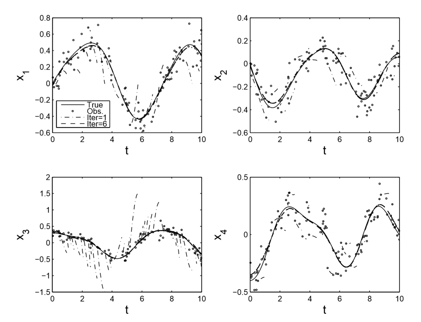
Figure 1: Initial and optimal trajectory corresponding to the Henon-Heiles system with estimated initial condition $\widehat{\mathbf{x}}_{0}=(-0.0231,-0.0008,0.3055,-0.3899)$ and parameters $\widehat{\mathbf{p}}=(1.0314,0.9839,-1.0101)$  and $\widehat{\sigma}=0.1029$.

Example 2. Consider the FitzHugh-Nagumo ODE, which is a simplified version of the well-known Hodgkin–Huxley model for describing activation and deactivation dynamics of a spiking neuron:

$$\overset{.}{V} = c(V-\frac{V^{3}}{3}+R)$$

$$\overset{.}{R} = -\frac{1}{c}(V-a+bR),$$

where $V$ and $R$ denote the voltage across an axon membrane and the outwards currents, respectively. Here, $a,b,c$ are parameters to be estimated from $n=400$ noisy observations of the variable $V$, which were randomly distributed (with uniform distribution) in the interval $[0,20]$. Similarly to [12] and [8], the true trajectory was generated with initial values $V(0)=-1$ and $R(0)=1$ and true parameters $\ a=0.2$, $b=0.2$ and $c=3$. The noisy observations were generated by adding a Gaussian noise with standard deviation $\sigma$ $=0.2$. The initial parameter guess was set $\mathbf{p}^{(0)}=(a^{(0)},b^{(0)},c^{(0)})=(2,2,5)$ and $\sigma^{(0)}=1$. A number of $m=50$ shooting nodes were approximately equispaced over the set of observation time points. Since only the variable $V$ is observed in the case and no additional information if available for the variable $R$ at the shooting points, we set the second component of $\mathbf{s}_{k}^{(0)}$ equal to zero for all $k=0,...,m$.

The estimated parameters resulting from 1000 realizations (20 batches of 50 realizations each) were $\widehat{a}=0.2007\pm 0.0023$, $\widehat{b}=0.1932\pm 0.0068$, $\widehat{c}=2.9794\pm 0.0113,\widehat{\mathbf{x}}_{0}=(-1.0019\pm 0.0123,1.0085\pm 0.0121)$ and $\widehat{\sigma}=0.2016\pm 0.0010$. Figure 2 shows the true, initial and estimated trajectories after $l=29$ iterations. Notice that a larger number of iterations were required in this case probably caused by the very bad (far away from the true trajectory) initial guess of the second component in the shooting nodes. The estimated trajectory corresponds to parameters with values $\widehat{a}=0.1971$, $\widehat{b}=0.2210$ and $\widehat{c}=2.9716.$

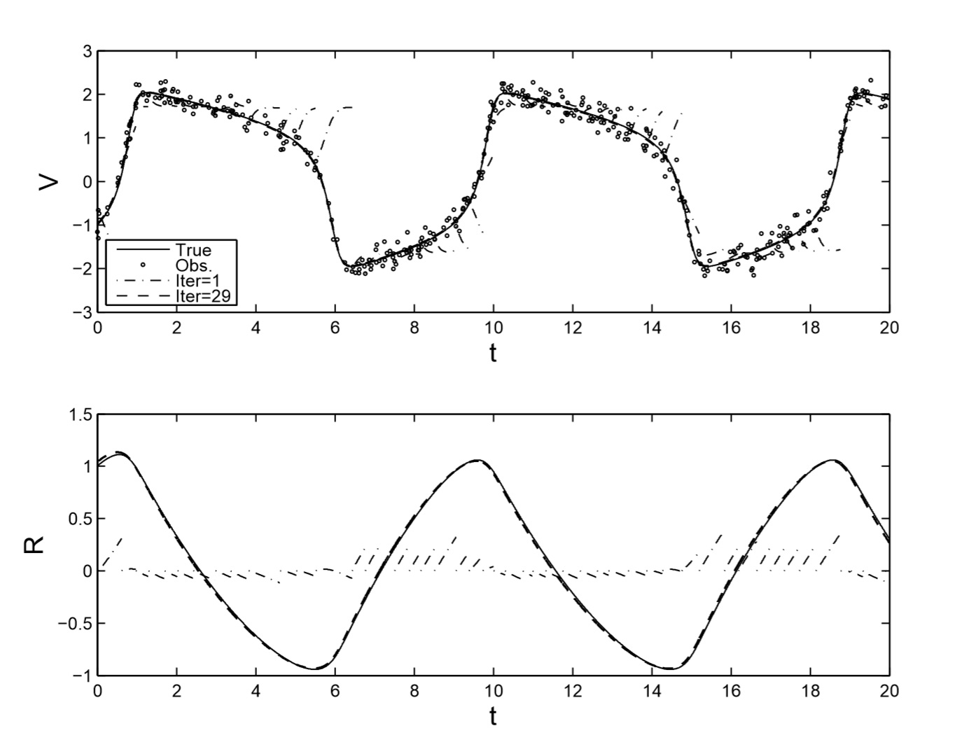
Figure 2: Initial and optimal trajectory corresponding to the FitzHugh-Nagumo system with estimated parameters $\widehat{a}=0.1971$, $\widehat{b}=0.2210$ and $\widehat{c}=2.9716.$

Example 3. Consider the Rikitake model defined by the ODE

$$\overset{.}{x}_{1} = -\mu x_{1}+x_{2}x_{3}$$

$$\overset{.}{x}_{2} = -\alpha x_{1}-\mu x_{2}+x_{1}x_{3}$$

$$\overset{.}{x}_{3} = 1-x_{1}x_{2},$$

which was originally introduced by [35] to explain geomagnetic polarity reversals. The model consists of coupled, self-excited disc dynamos, where the parameter $\mu>0$ and $\alpha$ represent the resistive dissipation and the difference of the angular velocities of two dynamo discs, respectively. Despite the physical meaning of $\mu$ is still not clear, estimates of geophysically plausible value for $\mu$ vary between $10^{-3}$ and $10$ [36]. Most of the studies for explaining the dynamical behavior of the Rikitake system focus on the parameter space determined by the pairs  $(\mu,K)\,$, where $\alpha=\mu(K^{2}-K^{-2})~{}$(see [36] for instance). Thus, combinations of the pairs $(\mu,K)$ produce different dynamical regimes, like the chaotic regime determined by $\mu=0.5$ and $\alpha=0.46125$ $(K=1.25).$

For this example, the parameters $\mu$ and $\alpha$ are going to be estimated from $N=200$ noisy observations of the three variable, randomly distributed (with uniform distribution) in the interval $[0,40]$. A ”true” trajectory was simulated with initial value $\mathbf{x}_{0}=(-2,-2,0)$ and the noisy observations were generated by adding a Gaussian noise with standard deviation $\sigma$ $=0.1.$ The initial parameter guesses were set at $\mathbf{p}^{(0)}=(\mu^{(0)},\alpha^{(0)})=(5,5)$ and $\sigma^{(0)}=1$. The following table presents the estimated parameters for different numbers of shooting nodes, including the case $m=0$ corresponding to the Initial Value approach. The estimated parameters are reported by the average and standard deviation over 100 different realizations of the observations $\mathbf{z}_{i}$ with a fix (random) distribution of the $N$ observation time points $t_{i}^{\ast}$, $i=1,...,N$. Notice that the average and standard deviation were calculated only across those realizations where the estimation algorithm converged after a maximum number of 50 iterations. In fact, this table also shows the required number of Gauss-Newton iterations ($N.Iter.$) that the algorithm needed to converge as well as the percentage of convergence ($\%Conv.$).

$$\text{Table 2. Estimated parameters, number of required Gauss-Newton iterations (}N.Iter.\text{), }$$

$$\text{and percentage of convergence (}\%Conv.\text{) corresponding to the Rikitake system.}$$

Notice that as the number of shooting nodes decreases, the estimated parameters become less accurate and the number of non convergent realizations increases. In fact, the simulations corresponding to $m=10$ and $m=0$ showed no convergent realization at all, which evidences the efficacy of the multiple shooting method as compared to the Initial Value approach. Importantly, recall that, due to the equivalent condensed problem, increasing the number of shooting nodes does not increase the dimensionality of the optimization problem. Therefore, as a rule of thumb, it is recommendable to employ the multiple shooting approach with a relatively large number of shooting nodes, particularly for those system showing complex, chaotic dynamics.

5 Discussion

The methodology presented here can be extended in several ways. As it was mentioned earlier, only the case of equality constrains for parameters and state variables has been treated here. For inequality constrains, it is easy to check that the condensing recursion is exactly the same as for equality constrains. Therefore, the solution of the condensed problem must be obtained by more general optimization strategies like active set strategy (see details in [6] and [7]). Additionally, we have assumed a very simple assumption for the measurements errors that define the set of observed data points. Namely, uncorrelated and equally distributed errors have been assumed for the components of the multi-dimensional data. This scenario can be easily extended to the more general case of correlated errors by replacing the parameter $\sigma^{2}$ by a variance-covariance matrix $\Sigma~{}$ and defining a proper formulation of the function $\mathbf{F}_{1}(\mathbf{p})$. Correspondingly, the observed data and the measurements errors might define more complicated statistical models like mixed effects models to cover, for instance, the cases of repeated measures at certain time points and temporarily-correlated errors.

Finally, the multiple shooting-LL approach can covers a more general class of models driven by random differential equations (RDE). Essentially, a RDE is a non autonomous ODE coupled with a stochastic process, which is usually employed for modelling noisy perturbations of deterministic systems. Thus, in principle, a RDE can be integrated by applying conventional numerical methods for ODEs, like the LL integrator presented here [37]. In fact, the LL method for RDE has been already successfully applied for the generation of EEG rhythms by means of realistically coupled neural mass models [38]. A possible extension consists of having more realistic neural mass models with certain free parameters that could be estimated from observed EEG data via the multiple shooting approach.

6 Conclusions

In this paper we have shown the feasibility of the multiple shooting approach in combination with local linearization techniques for parameter estimation in ordinary differential equations. The main advantage of the proposed approach consists of approximating the numerical derivatives involved in the multiple shooting scheme by a numerically stable method at no extra computational burden but the one required for the numerical integration of the original equations. The performance of the proposed approach has been evaluated in three different numerical examples. In all cases, the multiple shooting-local linearization method accurately recovered the true parameters values.

References

- [1] C. Chicone, Ordinary differential equations with applications, Springer Verlag, New York, 2006.
- [2] E. Baake, M. Baake, H. Bock, K. Briggs, Fitting ordinary differential equations to chaotic data, Physical Review A 45 (8) (1992) 5524–5529.
- [3] J. Kallrath, J. Schlöder, H. Bock, Least squares parameter estimation in chaotic differential equations, Celestial Mechanics and Dynamical Astronomy 56 (1993) 353–371.
- [4] H. Voss, J. Timmer, J. Kurths, Nonlinear dynamical system identification from uncertain and indirect measurements, International Journal of Bifurcation and Chaos 14 (6) (2004) 1905–1933.
- [5] H. Abarbanel, D. Creveling, Dynamical state and parameter estimation, SIAM Journal on Applied Dynamical Systems 8 (4) (2009) 1341–1381.
- [6] H. Bock, Numerical treatment of inverse problems in chemical reaction kinetics, Modelling of Chemical Reaction Systems 18 (1981) 102–125.
- [7] H. Bock, Recent advances in parameter identification techniques for ode, in: P. Deuflhard (Ed.), Numerical Treatment of Inverse Problems in Differential and Integral Equations, Birkhäuser, Boston, 1983, pp. 95–121.
- [8] J. Cao, L. Wang, J. Xu, Robust estimation for ordinary differential equation models, Biometrics 67 (4) (2011) 1305–1313.
- [9] D. Leineweber, I. Bauer, An efficient multiple shooting based reduced SQP strategy for large-scale dynamic process optimization. Part 1: theoretical aspects, Computers & Chemical Engineering 27 (2) (2003) 157–166.
- [10] M. Peifer, J. Timmer, Parameter estimation in ordinary differential equations for biochemical processes using the method of multiple shooting, Systems Biology, IET 1 (2) (2007) 78 – 88.
- [11] J. Varah, A spline least squares method for numerical parameter estimation in differential equations, SIAM Journal on Scientific and Statistical Computing 3 (1) (1982) 28–46.
- [12] J. Ramsay, G. Hooker, Parameter estimation for differential equations: a generalized smoothing approach, Journal of the Royal Statistical Society: Series B 69 (5) (2007) 741–796.
- [13] N. Brunel, Parameter estimation of ODE’s via nonparametric estimators, Electronic Journal of Statistics 2 (2008) 1242–1267.
- [14] H. Wu, H. Xue, A. Kumar, Numerical Discretization-Based Estimation Methods for Ordinary Differential Equation Models via Penalized Spline Smoothing with Applications in Biomedical Research, Biometrics 68 (2) (2012) 344–352.
- [15] E. Hairer, S. P. Norsett, G. Wanner, Solving Ordinary Differential Equations I: Nonstiff Problems, 2nd Edition, Springer, 2008.
- [16] J. C. Jimenez, R. Biscay, C. Mora, L. M. Rodriguez, Dynamic properties of the local linearization method for initial-value problems, Applied Mathematics and Computation 126 (1) (2002) 63–81.
- [17] J. C. Jimenez, F. Carbonell, Rate of convergence of local linearization schemes for initial-value problems, Applied Mathematics and Computation 171 (2) (2005) 1282–1295.
- [18] L. Pedroso, A. Marrero, H. de Arazoza, Nonlinear Parametric Model Identification using Genetic Algorithms, Lecture Notes in Computer Sciences 2867 (2003) 473–480.
- [19] S. Donnet, A. Samson, Estimation of parameters in incomplete data models defined by dynamical systems, Journal of Statistical Planning and Inference 137 (9) (2007) 2815–2831.
- [20] J. Ginart, A. Marrero, M. L. Baguer, H. de Arazoza, Parameter Estimation in HIV/AIDS Epidemiological Models, Revista de Matemática: Teoría y Aplicaciones 17 (2010) 143–158.
- [21] F. Carbonell, J. C. Jimenez, R. J. Biscay, A numerical method for the computation of the Lyapunov exponents of nonlinear ordinary differential equations, Applied Mathematics and Computation 131 (1) (2002) 21–37.
- [22] R. F. Hartl, S. P. Sethi, R. G. Vickson, A Survey of the Maximum Principles for Optimal Control Problems with State Constraints, SIAM Review 37 (2) (1995) 181–218.
- [23] J. Stoer, On the numerical solution of constrained least-squares problems, SIAM Journal on Numerical Analysis 8 (2) (1971) 382–411.
- [24] R. Hanson, K. Haskell, Algorithm 587: Two algorithms for the linearly constrained least squares problem, ACM Transactions on Mathematical Software 8 (3) (1982) 323–333.
- [25] R. Hanson, Linear least squares with bounds and linear constraints, SIAM Journal on scientific and statistical computing 7 (3) (1986) 826–834.
- [26] P. Deuflhard, A modified Newton method for the solution of ill-conditioned systems of nonlinear equations with application to multiple shooting, Numerische Mathematik 22 (1974) 289–315.
- [27] M. Al-Baali, R. Fletcher, An efficient line search for nonlinear least squares, Journal of Optimization Theory and Applications 48 (3) (1986) 359–377.
- [28] J. Moré, D. Thuente, Line search algorithms with guaranteed sufficient decrease, ACM Transactions on Mathematical Software 20 (3) (1994) 286–307.
- [29] H. Zhang, W. Hager, A nonmonotone line search technique and its application to unconstrained optimization, SIAM Journal on Optimization 14 (4) (2004) 1043–1056.
- [30] A. Sotolongo, J. C. Jiménez, Construction and study of local linearization adaptive codes for ordinary differential equations., Revista de Matemática: Teoría y Aplicaciones 21 (1) (2014) 21–53.
- [31] F. Carbonell, J. C. Jímenez, L. M. Pedroso, Computing multiple integrals involving matrix exponentials, Journal of Computational and Applied Mathematics 213 (1) (2008) 300–305.
- [32] G. H. Golub, C. F. V. Loan, Matrix Computations, third edit Edition, The Johns Hopkins University Press, 1996.
- [33] R. B. Sidje, Expokit: a software package for computing matrix exponentials, ACM Transactions on Mathematical Softwares 24 (1) (1998) 130–156.
- [34] C. Van Loan, Computing integrals involving the matrix exponential, IEEE Transactions on Automatic Control, 23 (3) (1978) 395–404.
- [35] T. Rikitake, Oscillations of a system of disk dynamos, Mathematical Proceedings of the Cambridge Philosophical Society 54 (1) (1958) 89–105.
- [36] K. Ito, Chaos in the Rikitake two-disc dynamo system, Earth and Planetary Science Letters 51 (2) (1980) 451–456.
- [37] F. Carbonell, J. C. Jimenez, R. J. Biscay, H. De La Cruz, The local linearization method for numerical integration of random differential equations, BIT Numerical Mathematics 45 (1) (2005) 1–14.
- [38] R. C. Sotero, N. J. Trujillo-Barreto, Y. Iturria-Medina, F. Carbonell, J. C. Jimenez, Realistically coupled neural mass models can generate EEG rhythms., Neural computation 19 (2) (2007) 478–512.