Enhancing efficiency and power of quantum-dots resonant tunneling thermoelectrics in three-terminal geometry by cooperative effects

Abstract

We propose a scheme of multilayer thermoelectric engine where one electric current is coupled to two temperature gradients in three-terminal geometry. This is realized by resonant tunneling through quantum dots embedded in two thermal and electrical resisting polymer matrix layers between highly conducting semiconductor layers. There are two thermoelectric effects, one of which is pertaining to inelastic transport processes (if energies of quantum dots in the two layers are different) while the other exists also for elastic transport processes. These two correspond to the transverse and longitudinal thermoelectric effects respectively and are associated with different temperature gradients. We show that cooperation between the two thermoelectric effects leads to markedly improved figure of merit and power factor which is confirmed by numerical calculation using material parameters. Such enhancement is robust against phonon heat conduction and energy level broadening. Therefore we demonstrated cooperative effect as an additional way to effectively improve performance of thermoelectrics in three-terminal geometry.

I Introduction

Harvesting usable energy from wasted heat using thermoelectrics has been attracting a lot of research interest.honig Much efforts have been devoted to bulk materials, making them mature thermoelectric systems that are already useful in industrial technologies.rev ; rev2 Recently there is a trend of incorporating nanostructures to further improve the performance of thermoelectric materials.nano1 ; nano2 ; lowd Successful examples have been achieved in many materials/structures along this direction.nano1 ; nano2 ; lowd Theoretical studies have demonstrated that the thermoelectric properties of individual nanostructures can be much better than the bulk.joe ; hicks ; ms ; Linke Experimental efforts have pushed forward the measurements of thermoelectric properties of individual nanostructures.nano-exp ; nano-th There are also studies trying to fill the gaps between the thermoelectric properties of individual nanostructures and their assembliesnano1 ; nano2 ; lowd as well as attempts to improve thermoelectric performance by tuning the shape and organization patterns of nanostructures.nano-ordering

In addition to material and structural aspects, geometry also plays an important role in thermoelectric applications. For example, transverse thermoelectricsTTE take advantages of accumulating temperature difference in one direction while generating electric current in the perpendicular direction. Geometric separation of the electric and heat flows facilitates special functions. For example, thermoelectric cooling and engine can be realized using a single type of carrier doping (i.e., without serial connection between $n$- and $p$-type thermoelectric components) via transverse thermoelectric effect.TTE Recently a related, but different, thermoelectric effect is found in mesoscopic thermoelectrics in three-terminal geometry.3t0 ; ora ; dot ; cavity ; prb1 ; photon ; magnon ; segal ; hopping ; jordan ; pn ; patent ; new ; qw Researches in this direction is pioneered by the theory of Edwards et al.Edwards and the later experiments.cam-exp The underlying physics is illustrated in Fig. 1 (see also Ref. prb1, ): excess population of phonons can induce an electric current during inelastic transport processes. Heat and electric flows are geometrically separated since heat is carried by the phonons flowing from/into the phonon bath. This picture can be generalized to inelastic transport processes assisted by other elementary excitations, such as photonsphoton , electron-hole excitationsdot ; cavity and magnons.magnon Besides the quantum dots (QDs) can be replaced with any conductors given that the carrier energies at the left and right conductors are considerably different, which can be realized by two low-dimensional structures (e.g., quantum wellsqw or wires), or a barrier,patent or a band gap.pn

Figure 1: (Color online) Illustration of a three-terminal thermoelectric system (studied in Ref. prb1, ). (a) An electron first tunnels from the source to the quantum dot (represented by a red dot) with energy $E_{1}$ and then hops to the other quantum dot with energy $E_{2}$ by absorbing a phonon from the phonon bath. After that the electron tunnels into the drain electrode. The tunneling processes are elastic, while the hoping between quantum dots must be assisted by a phonon with energy $E_{2}-E_{1}>0$. The temperatures of the source, drain and phonon bath are $T_{s}$, $T_{d}$, and $T_{p}$, while the electrochemical potentials of the source and drain are $\mu_{s}$ and $\mu_{d}$, respectively. When the phonon bath has the highest temperature among the three reservoirs, excess number of phonons prefer phonon absorption processes and hence induces an electric current from the source to the drain. (b) In realistic situations the phonon bath is connected with the (insulating) substrate supporting the quantum dots while the two electrodes are suspended to be isolated from the phonon bath.

Microscopic analysis3t0 ; dot ; cavity ; prb1 ; photon ; magnon ; jordan ; pn ; patent ; new ; qw indicates that the performance of each individual nano-scale three-terminal thermoelectric (3T-TE) device is promising. Experiments have demonstrated the effectiveness of 3T-TE cooling at submicron scale.cam-exp In this work we focus on 3T-TE systems based on the structure illustrated in Fig. 2. This structure was initially proposed by Edwards et al.Edwards and later explored experimentally in Ref. cam-exp, for cooling of electrons at cryogenic temperature. Recently Jordan et al. extend the idea to thermoelectric engine with layered self-assembled QDs where considerable electrical current density could be obtained due to contributions from many parallel quantum tunneling channelsjordan . This proposal significantly improve the potential for thermoelectric energy harvesting of the original idea (An extended idea of replacing the QD layers by quantum wells is presented in Ref. qw, ). Here we exploit the same structure of Jordan et al. to study cooperative effects between the longitudinal and transverse thermoelectric powers.

In Fig. 2(a) the electronic cavity, as well as the source and the drain, are highly conducting layers made of heavily-doped semiconductors (e.g., heavily-doped silicon or GaAs). In between those layers, there are two highly resisting layers with high thermal and electrical resistance. Each of the resisting layer is embedded with a QD through which electrons can tunnel between the cavity and the electrodes. The resonant tunneling through QDs are responsible for the transport. The energy levels in the left and right QDs are $E_{1}$ and $E_{2}$, respectively. When $E_{1}\neq E_{2}$, an electron transmitting from the source to the drain takes a finite amount of energy, $E_{2}-E_{1}$, from the cavity. To reach steady states the cavity must exchange energy with the phonon bath [see Fig. 2(b)]. The transverse thermoelectric effect is manifested as the fact that an electric current drives a heat current from the phonon bath [see Fig. 2(b)], and vice versa.

Following Ref. jordan, , the scheme to assemble the nano-scale devices into a macroscopic device is straightforward: 2D arrays of QDs can be placed in the resisting layers [see Fig. 2(c)]. This can be realized by self-assembled QDs grown on the surface of semiconductors,ass-qd or as we proposed here, core-shell QDs embedded in (undoped) polymers with low thermal and electrical conductance.polymer ; poly ; poly2 ; note1 In such an assembly scheme the total electric current is the sum of the electric currents in each nano-scale 3T-TE device (i.e., a pair of QDs). High power density can be prompted by high density of QDs which can reach $\sim 10^{11}$ cm^-2 for a single layer (about 1 nm thick).ass-qd

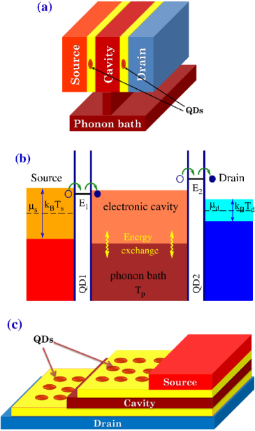
Figure 2: (Color online) Illustration of the 3T-TE device studied in this work. (a) Schematic of a possible realistic set-up. The layered structure consists of three highly conducting regions: the source, cavity, and drain. In between them there are two highly resisting layers (yellow regions) with very low thermal and electrical conductance. A QD is embedded into each resisting layer to allow electrical and thermal conduction through it. The cavity is connected with a (insulating) phonon bath. The connection allows efficient energy exchange between them. (b) Illustration of the microscopic processes. Carrier distributions in the source and the drain are determined by the chemical potentials and temperatures. Electrons transmit through QDs via resonant tunneling. When energies of the two QDs, $E_{1}$ and $E_{2}$, are different, energy exchange between the cavity and the phonon bath is necessary for the establishment of the steady state transport. (c) A scheme for building macroscopic devices where many QDs, forming 2D arrays, are embedded in the resisting layers.

To date all works on 3T-TE systems focus on exploiting the transverse thermoelectric effect. However, there is also a longitudinal thermoelectric effect in the system: the temperature difference between the two electrodes can also induce an electric current. A full description of thermoelectric transport in 3T-TE systems is given by the phenomenological equation (similar equations were found in Refs. ora, ; prb1, ; pn, ; hopping, )

$$\left(\begin{array}[]{c}I\\ I_{Q1}\\ I_{Q2}\end{array}\right)=\left(\begin{array}[]{cccc}G&L_{1}&L_{2}\\ L_{1}&K_{1}&K_{12}\\ L_{2}&K_{12}&K_{2}\\ \end{array}\right)\left(\begin{array}[]{c}V\\ \Delta T_{1}/T\\ \Delta T_{2}/T\end{array}\right),$$ (1)

where $L_{1}$ and $L_{2}$ represent the longitudinal and transverse thermoelectric effects, respectively. $I_{Q1}$ and $I_{Q2}$ stand for the heat currents leaving the source and the phonon bath, respectively. The two temperature differences are $\Delta T_{1}=T_{s}-T_{d}$ and $\Delta T_{2}=T_{p}-T_{d}$ with $T_{s}$, $T_{d}$, and $T_{p}$ being the temperatures of the source, the drain, and the phonon bath, respectively.

In this work we show that, if both the longitudinal and transverse thermoelectric effects are exploited simultaneously, due to cooperation between the two, the efficiency and power can be considerably improved. The cooperative effect originates deeply from the nature of three-terminal thermoelectric systems: the two thermoelectric effects are correlated with each other, or in other words, the electrical current are simultaneously induced by the two different temperature gradients. Simplified geometric interpretation is that the electric currents induced by the two thermoelectric effects can be parallel or anti-parallel. In the former case the two effects add up constructively, leading to enhanced thermopower and efficiency. The phenomenon reflects the cooperative effect of two (or more) correlated thermoelectric effects which is referred to as the “cooperative thermoelectric effect”.

The cooperative thermoelectric effect is manifested in the proposed thermoelectric device. Using material parameters we calculate the thermoelectric transport coefficients as well as the figure of merit and power factor. It is found that both the figure of merit and the power factor are considerably improved by the cooperative thermoelectric effect. This enhancement is as effective for good thermoelectrics as that for bad thermoelectrics. In calculation we show that the enhancement induced cooperative effect changes only slightly when phonon heat conductivity or QD energy broadening is increased significantly. These results demonstrate that cooperative effect is an alternative way to improve the performance of thermoelectrics in three-terminal geometry effectively.

This paper is organized as follows: In Sec. II we establish thermoelectric transport of the 3T-TE systems from microscopic theory. In Sec. III we demonstrate the cooperative thermoelectric effect in a geometric way. In Sec. IV we calculate the thermoelectric transport coefficients as well as the figures of merit and power factors for the longitudinal, transverse, and cooperative thermoelectric effects for the 3T-TE systems using material parameters. We conclude in Sec. V. Studies in this work are focused on linear-response steady state transport. Interesting nonlinear effectsnonl could be discussed in future works.

II Microscopic theory of Thermoelectric transport

In this section we develop a microscopic theory of 3T-TE transport, following the formalism of Jordan et al.jordan The system is a layered structure with thickness $L_{tot}=L_{s}+L_{d}+L_{c}+2L_{qd}$ where $L_{s}$, $L_{d}$, $L_{c}$, and $L_{qd}$ are the thickness of the source, the drain, the cavity, and the resisting layers, respectively. For realistic design, $L_{s}$, $L_{d}$, and $L_{c}$ is about one hundred nanometers (nm), while $L_{qd}$ is on the order of ten nm. The size of QDs is a few nm. The level spacing of the QDs, typically on the order of 100 meV for core-shell QDs (see Ref. gong, ), is much larger than $k_{B}T$. We suggest to fabricate serially connected unit structures [the structure in Fig. 2(a)] to scale the device up to a fully three-dimensional macroscopic device which can be implemented via layer-by-layer growth methods.

The Hamiltonian of the system is written as

$$H=H_{s}+H_{d}+H_{c}+H_{qd}+H_{int},$$ (2)

where $H_{s}$, $H_{d}$, $H_{c}$, and $H_{qd}$ are the Hamiltonian of the source, the drain, the cavity, and the QD, respectively. $H_{\alpha}=\sum_{\vec{k}}\varepsilon_{\vec{k}}c^{\dagger}_{{\vec{k}},\alpha}c_{{\vec{k}},\alpha}$, where $\alpha=s,d,c$ denotes the source, the drain, and the cavity, respectively. $\varepsilon_{\vec{k}}=\frac{\hbar^{2}k^{2}}{2m^{\ast}}$ with $m^{\ast}$ being the effective mass of the charge carrier.

$$H_{qd}=\sum_{i}E_{i}^{(\ell)}d_{i}^{\dagger}d_{i}+\sum_{j}E_{j}^{(r)}d_{j}^{\dagger}d_{j},$$ (3)

where the index $i$ and $j$ numerate the QDs in the left $({\ell})$ and right $(r)$ resisting layers, respectively. $H_{int}$ describes hybridization of the QD states with the states in the source, drain, and cavity,

$$H_{int}=\sum_{\alpha=s,c}\sum_{{\vec{k}},i}V^{(\ell)}_{i,\alpha,{\vec{k}}}c^{\dagger}_{{\vec{k}},\alpha}d_{i}+\sum_{\alpha=d,c}\sum_{{\vec{k}},j}V^{(r)}_{j,\alpha,{\vec{k}}}c^{\dagger}_{{\vec{k}},\alpha}d_{j}+{\rm H.c.}$$ (4)

The electric and thermal currents through the left resisting layer from the source to the cavity are given bybook

$$I_{e,\ell} =\frac{2e}{h}\int dE\ t_{\ell}(E)[f_{s}(E)-f_{c}(E)],$$ (5a)

$$I_{Q,\ell} =\frac{2}{h}\int dE(E-\mu)t_{\ell}(E)[f_{s}(E)-f_{c}(E)],$$ (5b)

respectively. The factor of two comes from the spin degeneracy of the carriers. $e$ is the electronic charge. $f_{s}$ and $f_{c}$ are the carrier distribution functions of the source and the cavity, respectively. They are determined by the temperatures of the source $T_{s}$ and the cavity $T_{c}$ as well as by their electrochemical potentials $\mu_{s}$ and $\mu_{c}$. Note that because the voltage and temperature gradients are mainly distributed at the two resisting layers, as a good approximation, one can assign uniform chemical potentials and temperatures to the source, drain, and cavity regions. The energy dependent transmission through QDs is given bybook ; ora $t_{\ell}(E)=\sum_{i}t_{i}(E)$ with

$$t_{i}(E)=\frac{\hbar^{2}\Gamma_{s,i}(E)\Gamma_{c,i}^{(\ell)}(E)}{(E-E_{i}^{(\ell)})^{2}+\frac{\hbar^{2}}{4}\left(\Gamma_{s,i}(E)+\Gamma_{c,i}^{(\ell)}(E)\right)^{2}},$$ (6)

where

$$\Gamma_{s,i}(E)=\frac{2\pi}{\hbar}\sum_{\vec{k}}|V^{(\ell)}_{i,s,{\vec{k}}}|^{2}\delta(E-\varepsilon_{\vec{k}}),$$ (7a)

$$\Gamma_{c,i}^{(\ell)}(E)=\frac{2\pi}{\hbar}\sum_{\vec{k}}|V^{(\ell)}_{i,c,{\vec{k}}}|^{2}\delta(E-\varepsilon_{\vec{k}}),$$ (7b)

are the energy-dependent tunneling rates from the QD $i$ to the source and the cavity, respectively. The electric and thermal currents from the drain to the cavity can be obtained by the replacements: $i\to j$, $\ell\to r$, and $s\to d$. Introducing

$$G_{\ell} =\frac{2e^{2}}{hk_{B}T}\int dE\ t_{\ell}(E)f(E)[1-f(E)]$$ (8a)

$$L_{\ell} =\frac{2e}{hk_{B}T}\int dE(E-\mu)t_{\ell}(E)f(E)[1-f(E)]$$ (8b)

$$K_{\ell} =\frac{2}{hk_{B}T}\int dE(E-\mu)^{2}t_{\ell}(E)f(E)[1-f(E)]$$ (8c)

with $f(E)$ being the equilibrium carrier distribution, in the linear-response regime one can rewrite Eq. (5) as

$$I_{e,\ell} =G_{\ell}(\mu_{s}-\mu_{c})/e+L_{\ell}(T_{s}-T_{c})/T,$$ (9a)

$$I_{Q,\ell} =L_{\ell}(\mu_{s}-\mu_{c})/e+K_{\ell}(T_{s}-T_{c})/T.$$ (9b)

Expressions for the currents from the drain to the cavity $I_{e,r}$ and $I_{Q,r}$ can be obtained from the above by the replacements $\ell\to r$ and $s\to d$.

Inelastic scatterings, such as the electron-phonon and electron-electron scatterings, are crucial for the establishment of steady states in the cavity. In the concerned temperature range, $300\sim 500$ K, those scatterings are quite efficient. The heat transfer between the phonon bath and the cavity can be made efficient by using materials with high thermal conductivity to connect them. Interface thermal resistance can be reduced if the cavity and the phonon bath are made of the same material. We assume the thermal conduction between the phonon bath and the cavity is efficient and the temperature gradient across them and within the cavity is considerably smaller than that across the two polymer layers. In this way the temperature of the cavity is very close to that of the phonon bath and one can approximate that $T_{c}=T_{p}$.prb1 ; pn

Energy conservation gives $I_{Q,\ell}+I_{Q,r}+I_{Q,t}+IV=0$, where $I_{Q,t}$ is the heat current from the phonon bath to the cavity. Therefore there are only two independent heat currents.prb1 ; hopping In Eq. (1) the two independent heat currents are chosen as $I_{Q1}=I_{Q,\ell}$ and $I_{Q2}=I_{Q,t}$. Charge conservation, $I_{e,\ell}+I_{e,r}=0$, determines the electrochemical potential of the cavity

$$\mu_{c} = (G_{\ell}+G_{r})^{-1}\Big{\{}G_{\ell}\mu_{s}+G_{r}\mu_{d}+eT^{-1}\big{[}L_{\ell}\left(T_{s}-T_{p}\right)$$ (10)

$$\ \ +L_{r}\left(T_{d}-T_{p}\right)\big{]}\Big{\}}.$$

Inserting the above into Eqs. (1) and (9) we obtain

$$G=(G_{\ell}^{-1}+G_{r}^{-1})^{-1},\quad L_{1}=G\frac{L_{\ell}}{G_{\ell}},$$ (11a)

$$L_{2}=G(\frac{L_{r}}{G_{r}}-\frac{L_{\ell}}{G_{\ell}}),\quad K_{1}=K_{\ell}-\frac{L_{\ell}^{2}}{G_{\ell}+G_{r}},$$ (11b)

$$K_{12}=\frac{L_{\ell}(L_{\ell}+L_{r})}{G_{\ell}+G_{r}}-K_{\ell},$$ (11c)

$$K_{2}=K_{\ell}+K_{r}-\frac{(L_{\ell}+L_{r})^{2}}{G_{\ell}+G_{r}}.$$ (11d)

To understand these results, we rewrite the transport coefficients in terms of average electronic energies, following Mahan and Sofo,ms

$$L_{1} =e^{-1}G\left\langle E-\mu\right\rangle_{\ell},\ \ L_{2}=e^{-1}G(\left\langle E\right\rangle_{r}-\left\langle E\right\rangle_{\ell}),$$ (12a)

$$K_{1} =\frac{L_{1}^{2}}{G}+K_{tl},\quad K_{12}=\frac{L_{1}L_{2}}{G}-K_{tl},$$ (12b)

$$K_{2} =\frac{L_{2}^{2}}{G}+K_{tl}+K_{tr}.$$ (12c)

where

$$K_{tl} =e^{-2}G_{\ell}\Big{[}\left\langle(E-\mu)^{2}\right\rangle_{\ell}-\left\langle E-\mu\right\rangle^{2}_{\ell}\Big{]},$$ (13a)

$$K_{tr} =e^{-2}G_{r}\Big{[}\left\langle(E-\mu)^{2}\right\rangle_{r}-\left\langle E-\mu\right\rangle^{2}_{r}\Big{]}.$$ (13b)

The average in the above is defined as

$$\left\langle E^{n}\right\rangle_{\beta}\equiv\frac{\int dEE^{n}G_{\beta}(E)}{\int dEG_{\beta}(E)}$$ (14)

with $G_{\beta}(E)=\frac{2e^{2}}{hk_{B}T}t_{\beta}(E)f(E)[1-f(E)]$, for $\beta=\ell,r$ and $n=0,1,2$. $G_{\ell}=\int dEG_{\ell}(E)$ and $G_{r}=\int dEG_{r}(E)$. One readily notices from Eq. (13) that $K_{tl}$ and $K_{tr}$ must be non-negative.

For a macroscopic system with area $A$ the electrical conductivity is $\sigma=Gl_{u}/A$ with $l_{u}=2l_{qd}+l_{c}+(l_{s}+l_{d})/2$ being the thickness of an unit structure [the structure in Fig. 2(a)]. Similarly the thermal conductivities are $\kappa_{1}=K_{1}l_{u}/(AT)$, $\kappa_{2}=K_{1}l_{u}/(AT)$, and $\kappa_{12}=K_{12}l_{u}/(AT)$. The longitudinal and transverse thermopowers are

$$S_{1}\equiv\frac{L_{1}}{TG}=\frac{\left\langle E-\mu\right\rangle_{\ell}}{eT},\ \ S_{2}\equiv\frac{L_{2}}{TG}=\frac{\left\langle E\right\rangle_{r}-\left\langle E\right\rangle_{\ell}}{eT}.$$ (15)

$S_{2}$ is proportional to the energy difference, reflecting that it is associated with the inelastic processes. In contrary $S_{1}$ remains finite when inelastic processes vanish.

The total entropy production of the system in the linear response regime is written as

$$\frac{dS}{dt}=\frac{1}{T}\left(IV+I_{Q1}\frac{\Delta T_{1}}{T}+I_{Q2}\frac{\Delta T_{2}}{T}\right).$$ (16)

The second law of thermodynamics, $\frac{dS}{dt}\geq 0$, requires thatonsager

$$GK_{1}\geq L_{1}^{2},\ \ GK_{2}\geq L_{2}^{2},\ \ K_{1}K_{2}\geq K_{12}^{2},$$ (17)

as well as that the determinant of the $3\times 3$ transport matrix in Eq. (1) to be non-negative. Those requirements are satisfied for the transport coefficients in Eq. (12) because $K_{tl},K_{tr}\geq 0$.

III Cooperative effect: A geometric interpretation

We parametrize the two temperature differences as

$$\Delta T_{1}\equiv\Delta T\cos\theta,\quad\Delta T_{2}\equiv\Delta T\sin\theta.$$ (18)

The exergy efficiency (or the “second-law efficiency”, see Refs. 2nd, ; general, ) of the thermoelectric engine is2nd ; Odum ; general

$$\phi=\frac{-IV}{I_{Q1}\Delta T_{1}/T+I_{Q2}\Delta T_{2}/T}\leq\phi_{max}=\frac{\sqrt{ZT+1}-1}{\sqrt{ZT+1}+1}.$$

The exergy efficiency (“second-law efficiency”) is defined by the output free energy divided by the input free energy.2nd ; Odum ; general It has been widely used in the studies of energy conversion in chemical and biological systems since its invention about 60 years ago.Odum Recently it was applied to thermoelectric systemsrev2 . According to Ref. onsager, the rate of variation of free energy associated with a current is given by the product of the current and its conjugated thermodynamic force. Hence the denominator of the above equation consists of heat currents multiplied by temperature differences. It has been shown in Ref. general, that the relation between the efficiency of $\eta=W/Q$ for heat engine (or $\eta=Q/W$ for refrigerator) and the second-law efficiency $\phi$ is that $\phi=\eta/\eta_{C}$ where $\eta_{C}$ is the Carnot efficiency. Thus Ioffe’s figure of merit is also obtained starting from the second-law efficiency. At given $\theta$ the figure of merit is

$$ZT=\frac{\sigma S_{\rm eff}^{2}T}{\kappa_{\rm eff}-\sigma S_{\rm eff}^{2}T}$$ (19)

is the figure of merit. Here $S_{\rm eff}=S_{1}\cos\theta+S_{2}\sin\theta$ and $\kappa_{\rm eff}=(K_{1}\cos^{2}\theta+2K_{12}\sin\theta\cos\theta+K_{2}\sin^{2}\theta)l_{u}/(AT)$. Upon optimizing the output power of the thermoelectric engine, one obtainsmaxpower

$$W_{max}=\frac{1}{4}P(\Delta T)^{2},$$ (20)

with the power factor

$$P=\sigma S_{\rm eff}^{2}.$$ (21)

When $\theta=0$ or $\pi$, Eqs. (19) and (21) give the well-known figure of merit and power factor for the longitudinal thermoelectric effecthonig ; ms

$$Z_{l}T=\frac{\sigma S_{1}^{2}T}{\kappa_{1}-\sigma S_{1}^{2}T},\quad P_{l}=\sigma S_{1}^{2}.$$ (22)

The transverse thermoelectric figure of merit and power factor, i.e., $\theta=\pi/2$ or $3\pi/2$, are given byprb1 ; pn

$$Z_{t}T=\frac{\sigma S_{2}^{2}T}{\kappa_{2}-\sigma S_{2}^{2}T},\quad P_{t}=\sigma S_{2}^{2}.$$ (23)

Fig. 3(a) shows $ZT$ versus the angle $\theta$ in a polar plot for a specific set of transport coefficients satisfying the thermodynamic bounds in (17). Remarkably for $0<\theta<\pi/2$ and $\pi<\theta<3\pi/2$, $ZT$ is greater than both $Z_{l}T$ and $Z_{t}T$. To understand the underlying physics, we decompose the electric current into three parts $I=I_{0}+I_{1}+I_{2}$ with $I_{0}\equiv GV$, $I_{1}\equiv L_{1}\Delta T_{1}/T$, and $I_{2}=L_{2}\Delta T_{2}/T$. The two thermoelectric effects add up constructively when $I_{1}$ and $I_{2}$ have the same sign which takes place when $0<\theta<\pi/2$ and $\pi<\theta<3\pi/2$. Fig. 3(b) shows the power factor versus the angle $\theta$. The power factor is also larger when the two currents $I_{1}$ and $I_{2}$ are in the same direction. The cooperation of the two thermoelectric effects thus leads to enhanced figure of merit and output power.

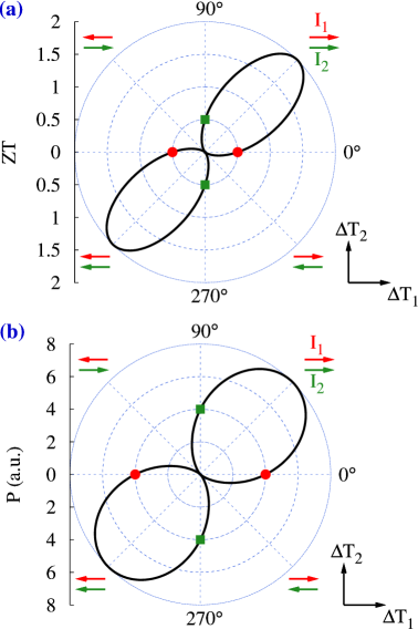
Figure 3: (Color online) Polar plot of figure of merit $ZT$ (a) and power factor $P$ (b) [in arbitrary unit (a.u.)] versus angle $\theta$. At $\theta=0^{\circ}$ or $180^{\circ}$ $ZT$ and $P$ recover the values for the longitudinal thermoelectric effect (red dots), while at $\theta=90^{\circ}$ and $270^{\circ}$ they go back to those of the transverse thermoelectric effect (green squares). The arrows in the I, II, III, IV quadrants label the direction of the currents $I_{1}\equiv L_{1}\Delta T_{1}/T$ (red arrows) and $I_{2}\equiv L_{2}\Delta T_{2}/T$ (green arrows). The transport coefficients are: $L_{1}=L_{2}=2Gk_{B}T/e$, $K_{1}=K_{2}=12G(k_{B}T/e)^{2}$, and $K_{12}=0$. $I_{0}\equiv GV$ (not shown) is reversed in III and IV quadrants for the operation of the thermoelectric engine.

One can maximize the figure of merit by tuning the angle $\theta$. This is achieved at

$$\partial_{\theta}(ZT)=0.$$ (24)

We find that the figure of merit is maximized at $\theta=\theta_{M}$ with

$$\tan(\theta_{M})\equiv\frac{L_{2}K_{1}-L_{1}K_{12}}{L_{1}K_{2}-L_{2}K_{12}}=\frac{S_{2}\kappa_{1}-S_{1}\kappa_{12}}{S_{1}\kappa_{2}-S_{2}\kappa_{12}}.$$ (25)

After some algebraic calculation the maximum figure of merit is found to be

$$Z_{M}T=\frac{G(K_{1}K_{2}-K_{12}^{2})}{D_{\cal M}}-1.$$ (26)

where $D_{\cal M}=GK_{1}K_{2}-GK_{12}^{2}-K_{2}L_{1}^{2}+2L_{1}K_{12}L_{2}-K_{1}L_{2}^{2}$ denotes the determinant of the $3\times 3$ transport matrix in Eq. (1). $Z_{M}T$ is greater than both $Z_{l}T$ and $Z_{t}T$, unless the denominator or the numerator in Eq. (25) vanishes. Nevertheless it is guaranteed by Eqs. (12) and (13) that both the numerator and denominator in Eq. (25) is nonzero when the broadening of the quantum dot energy is finite.

One can also tune $\theta$ to maximize the power factor $P$ which is achieved at

$$\partial_{\theta}P=0.$$ (27)

The power factor is maximized at $\theta=\theta_{m}$ (in general $\theta_{m}\neq\theta_{M}$) with

$$\tan(\theta_{m})\equiv\frac{L_{2}}{L_{1}}=\frac{S_{2}}{S_{1}}.$$ (28)

The maximum power factor

$$P_{m}=\sigma(S_{1}^{2}+S_{2}^{2})$$ (29)

is greater than both $P_{l}$ and $P_{t}$ unless $S_{1}$ or $S_{2}$ is zero. If $\theta_{M}$ is close to $\theta_{m}$, both the figure of merit and the power factor can be improved by the cooperative effect simultaneously in certain range of $\theta$.

The cooperative thermoelectric effect becomes particularly simple and vivid when $K_{12}=0$, $K_{1}=K_{2}\equiv K$, $L_{1}=L_{2}\equiv L$, and $S\equiv L/(TG)$. In this special case the transport equation becomes

$$\left(\begin{array}[]{c}I\\ I_{Q1}\\ I_{Q2}\end{array}\right)=\left(\begin{array}[]{cccc}G&L&L\\ L&K&0\\ L&0&K\\ \end{array}\right)\left(\begin{array}[]{c}V\\ \Delta T_{1}/T\\ \Delta T_{2}/T\end{array}\right).$$ (30)

We shall use the following combinations of temperature differences

$$\Delta T_{a}=\frac{\Delta T_{1}+\Delta T_{2}}{\sqrt{2}},\quad\Delta T_{b}=\frac{\Delta T_{1}-\Delta T_{2}}{\sqrt{2}}.$$ (31)

The heat currents conjugate to the above forces are

$$I_{Qa}=\frac{I_{Q1}+I_{Q2}}{\sqrt{2}},\quad I_{Qb}=\frac{I_{Q1}-I_{Q2}}{\sqrt{2}}.$$ (32)

The transport equation then becomes

$$\left(\begin{array}[]{c}I\\ I_{Qa}\\ I_{Qb}\end{array}\right)=\left(\begin{array}[]{cccc}G&\sqrt{2}L&0\\ \sqrt{2}L&K&0\\ 0&0&K\\ \end{array}\right)\left(\begin{array}[]{c}V\\ \Delta T_{a}/T\\ \Delta T_{b}/T\end{array}\right).$$ (33)

Consider conversion of heat $I_{Qa}$ into work $-IV$ at $\Delta T_{a}\neq 0$ and $\Delta T_{b}=0$. The figure of merit and power factor are

$$ZT=\frac{2L^{2}}{GK-2L^{2}}=\frac{2\sigma S^{2}T}{\kappa-2\sigma S^{2}T},\quad P=2\sigma S^{2},$$ (34)

respectively, with $\kappa\equiv Kl_{u}/(AT)$. The above figure of merit and power factor are greater than those of the longitudinal and transverse thermoelectric effects which are

$$Z_{l}T=Z_{t}T=\frac{\sigma S^{2}T}{\kappa-\sigma S^{2}T},\quad P_{l}=P_{t}=\sigma S^{2}.$$ (35)

IV Calculation of thermoelectric performance

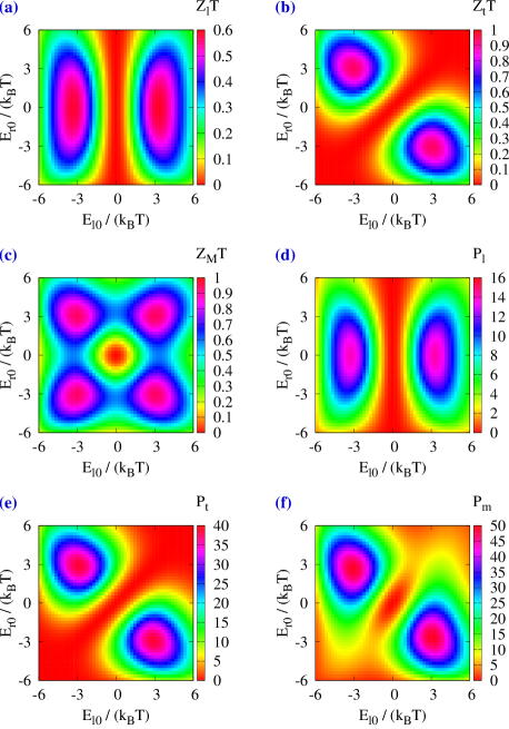
Figure 4: (Color online) Figures of merit $Z_{l}T$ (a), $Z_{t}T$ (b), and $Z_{M}T$ (c), and power factors (in unit of $10^{-4}$ W m^-1 K^-2) $P_{l}$ (d), $P_{t}$ (e), and $P_{m}$ (f) versus the QD energy $E_{\ell 0}$ and $E_{r0}$ for $\Delta_{qd}=20$ meV and $\kappa_{p}=0.05$ W m^-1 K^-1. The temperature is $T=400$ K, and the sheet density of QDs in each polymer layer (thickness 20 nm) is $4\times 10^{12}$ cm^-2. QD tunneling linewidth is $\Gamma=$30 meV.

We now calculate the transport coefficients using material parameters. The robustness of the device performance is tested by including the randomness of QD energy. Beside the transport mechanism described in Sec. II, there are other mechanisms conducting heat among reservoirs. The most important one is the heat conduction across the resisting layers by phonons. Polymers are good thermal insulators with heat conductivity $0.05\sim 1$ W m^-1 K^-1.polymer ; poly ; poly2 Phonon thermal conductivity should be much reduced in the nano-scale thin films concerned here due to abundant scattering with the embedded QDs and interfaces.nano1 We take the phonon thermal conductivity as $\kappa_{p}=0.05$ W m^-1 K^-1 (e.g., bulk rayonpolymer has thermal conductivity of 0.05 W m^-1 K^-1). The thermal conductance across a resisting layer is $K_{p}=A\kappa_{p}T/l_{qd}$. Adding this contribution to the transport equation and using Eq. (12) leads to

$$K_{1}=\frac{L_{1}^{2}}{G}+K_{tl}+K_{p},\quad K_{12}=\frac{L_{1}L_{2}}{G}-K_{tl}-K_{p},$$

$$K_{2}=\frac{L_{2}^{2}}{G}+K_{tr}+K_{tl}+2K_{p}.$$ (36)

The variance of the QDs energy is several tens of meV as revealed by experiments.ass-qd The thickness of the resisting layer is taken as $l_{qd}=20$ nm. The thickness of the source, the drain, and the cavity are all equal to 80 nm. High QD density, $2\times 10^{13}$ cm^-2, has been realized in polymer matrices of thickness around 20 nm.poly It is favorable to have more than one layer of QDs in each resisting layer to enable sufficient electron tunneling. Serial tunneling through several QDs may happen in the transmission across the resisting layers with many QDs.Gurvitz We suggest to incorporate $\simeq 4\times 10^{12}$ cm^-2 QDs into a 20 nm polymer layer which corresponds to a volume density of QDs as $\simeq 2\times 10^{18}$ cm^-3 (average inter-dot distance $\simeq 8$ nm). Taking into account of finite QD size, the inter-dot tunneling linewidth is $1\sim 30$ meV depending on materials and structures which is taken as $30$ meV here (see experimental measured value of 30 meV in Ref. awsh, ). And we take $\Gamma\equiv\Gamma_{c,i}^{(\ell)}(E)=\Gamma_{c,j}^{(r)}(E)=\Gamma_{s,i}(E)=\Gamma_{d,j}(E)=30$ meV ($\forall i,j,E$) as the QD tunneling linewidth used in calculating the tunneling rate. We shall study how the performance of the device varies with the variance and the mean value of the energy of QDs. The random QD energy in the left (right) resisting layer is modeled by a Gaussian distribution centered at $E_{\ell 0}$ ($E_{r0}$) with a variance $\Delta_{qd}^{2}$,

$$g_{\beta}(E)=\frac{1}{\Delta_{qd}\sqrt{2\pi}}\exp\left[-\frac{(E-E_{\beta 0})^{2}}{2\Delta_{qd}^{2}}\right].$$ (37)

with $\beta=\ell,r$. The QD energy and size can be controlled by various chemicalpoly and physicalass-qd methods during growth. We consider situations with temperature $T=400$ K. The energy zero is set to be the equilibrium chemical potential. The band edge of the semiconductor that constitutes the source, drain, and cavity layers is 200 meV below the chemical potential (a typical value for heavily-doped semiconductors). The electrical conductivity, thermopowers, and thermal conductivities are calculated according to Eqs. (12), (13), and (14). Based on those transport coefficients we calculate the figures of merit and power factors, $Z_{l}T$, $Z_{t}T$, $Z_{M}T$ [Figs. 4(a), 4(b), and 4(c)], $P_{l}$, $P_{t}$, and $P_{m}$ [Figs. 4(d), 4(e), and 4(f)].

Fig. 4 indicates that the figure of merit $Z_{l}T$ is optimized at the two points $E_{\ell 0}\simeq\pm 3k_{B}T$ with $E_{r0}=0$, while $Z_{t}T$ is optimized at $E_{\ell 0}=-E_{r0}\simeq\pm 3k_{B}T$. These results, which are consistent with the results in Ref. jordan, , can be understood as the balance between large electrical conductivity, large thermopower, and small thermal conductivity in optimizing the figure of merit. The power factors, $P_{l}$ and $P_{t}$, are optimized at parameters similar to those of $Z_{l}T$ and $Z_{t}T$, respectively. We find that when $Z_{t}T$ is optimized, $Z_{M}T$ is only slightly larger than $Z_{t}T$. For other situations, $Z_{M}T$ is considerably greater than both $Z_{l}T$ and $Z_{t}T$. Particularly near the two points $E_{\ell 0}=E_{r0}\simeq\pm 3k_{B}T$, the enhancement of figure of merit induced by cooperative effect is significant. For the power factor, cooperative effect always leads to considerable enhancement of power factor, unless when $P_{l}$ or $P_{t}$ are close to zero.

The above results reveal that cooperative effects can effectively improve the figure of merit and power factor for thermoelectrics in three-terminal geometry. Such improvement is especially useful for systems of which the electronic structure has not been fully optimized. Hence cooperative effects offer an additional way to improve the performance of thermoelectrics that are potentially useful for realistic systems. We also note that the largest figure of merit and power factor for the longitudinal thermoelectric effect are $Z_{l}T=0.6$ and $P_{l}=1.6\times 10^{-3}$ W m^-1 K^-2 respectively, while the largest figure of merit and power factor for the transverse thermoelectric effect is $Z_{t}T=1$ and $P_{t}=4\times 10^{-3}$ W m^-1 K^-2 respectively. This result confirms the conclusion in Refs. prb1, ; pn, ; hopping, ; jordan, ; qw, that the transverse thermoelectric effect in three-terminal geometry is of potential advantages.

Figure 5: (Color online) Figures of merit $Z_{l}T$ (a), $Z_{t}T$ (b), and $Z_{M}T$ (c), and power factors (in unit of $10^{-4}$ W m^-1 K^-2) $P_{l}$ (d), $P_{t}$ (e), and $P_{m}$ (f) versus the variance of the QDs energy $\Delta_{qd}$ and the difference of the mean values of QD energy in the two resisting layers $E_{r0}-E_{\ell 0}$. Here $E_{r0}$ is varying while $E_{\ell 0}=110$ meV ($\simeq 3k_{B}T$) is fixed. The temperature is $T=400$ K, $\kappa_{p}=0.05$ W m^-1 K^-1, and the sheet density of QDs in each polymer layer (of thickness 20 nm) is $4\times 10^{12}$ cm^-2. QD tunneling linewidth is $\Gamma=30$ meV.

In order to check the robustness of the effect in realistic situations we discuss the effect of the broadening of QD energy $\Delta_{qd}$ and the energy difference $E_{r0}-E_{\ell 0}$ for $E_{\ell 0}=110$ meV ($\simeq 3k_{B}T$). Increase of the broadening of QD energy $\Delta_{qd}$ reduces the thermopower and increases the electronic heat conductivity. Therefore the figures of merit and power factors for the longitudinal, transverse, and cooperative thermoelectric effects are all reduced. From Fig. 5 one finds that considerably large figures of merit and power factors can still be obtained for broadening of QD energy up to 50 meV. In experiments the full width at half-maximum of photoluminescence spectra can be as small as 35 meV (i.e., the variance is 15 meV).ass-qd Thus the proposed device is of potential application values. Finally in the above discussions only one energy level in each QD is considered. Careful calculation with higher energy levels (100 meV higher) included indicates that the figure of merit and the power factor are even larger [see Appendix].

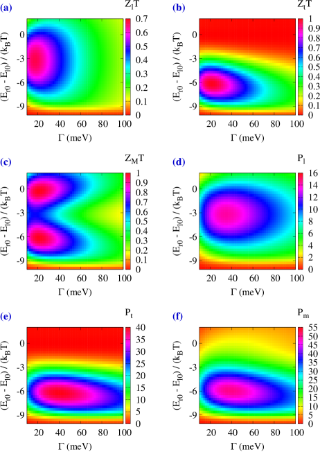
Figure 6: (Color online) Figures of merit $Z_{l}T$ (a), $Z_{t}T$ (b), and $Z_{M}T$ (c), and power factors (in unit of $10^{-4}$ W m^-1 K^-2) $P_{l}$ (d), $P_{t}$ (e), and $P_{m}$ (f) versus the tunneling linewidth of QDs $\Gamma$ and the difference of the mean values of QD energy in the two resisting layers $E_{r0}-E_{\ell 0}$. Here $E_{r0}$ is varying while $E_{\ell 0}=110$ meV ($\simeq 3k_{B}T$) is fixed. The temperature is $T=400$ K, $\kappa_{p}=0.05$ W m^-1 K^-1, and the sheet density of QDs in each polymer layer (of thickness 20 nm) is $4\times 10^{12}$ cm^-2. The variance of the QDs energy is $\Delta_{qd}=20$ meV.

We also plot the figures of merit and power factors for longitudinal, transverse, and cooperative thermoelectric effects as functions of the tunneling linewidth of QDs $\Gamma$ and the energy difference $E_{r0}-E_{\ell 0}$ for $E_{\ell 0}=110$ meV ($\simeq 3k_{B}T$) in Fig. 6. Unlike the monotonic dependence on the variance of the QDs energy $\Delta_{qd}$, the figures of merit and power factors first increases and then decreases with increasing $\Gamma$. This behavior is because at small $\Gamma$ increase of $\Gamma$ enhances electron tunneling and hence improves the electrical conductivity and the power factors. The enhancement of electron tunneling also improves electronic heat conductivity and reduces the effect of phonon heat conductivity on the figures of merit. Therefore, the figures of merit of the longitudinal, transverse, and cooperative thermoelectric effects are improved as well. However, the tunneling linewidth $\Gamma$ also induces broadening of the energy of transported electron. When such broadening is comparable with or larger than the thermal energy $k_{B}T$, it considerably reduces the thermopowers and increases the electronic thermal conductivity, hence the power factors $P_{l}$, $P_{t}$, and $P_{m}$ as well as the figures of merit $Z_{l}T$, $Z_{t}T$, and $Z_{M}T$ are reduced. The optimal tunneling linewidths for $Z_{l}T$, $Z_{t}T$, and $Z_{M}T$ are $\Gamma=17.3$, 21.4, 21.4 meV respectively where the optimal figures of merit are $Z_{l}T=0.668$, $Z_{t}T=0.987$, and $Z_{M}T=0.989$ respectively. Besides, the optimal tunneling linewidths for $P_{l}$, $P_{t}$, and $P_{m}$ are $\Gamma=34.5$, 39.4, and 38.6 meV respectively where the optimal power factors are $P_{l}=1.43\times 10^{-3}$ W m^-1 K^-2, $P_{t}=3.96\times 10^{-3}$ W m^-1 K^-2, and $P_{m}=5.02\times 10^{-3}$ W m^-1 K^-2 respectively. The optimal figure of merit and power factor for the cooperative thermoelectric effect are larger than those of the transverse and longitudinal thermoelectric effects. This result is consistent with the proof in Sec. III that the figure of merit and the power factor of the cooperative thermoelectric effect is greater than or equal to those of the longitudinal and transverse thermoelectric effects. Meanwhile the optimal performance of the transverse thermoelectric effect is also better than that of the longitudinal thermoelectric effect. Overall there are more parameter regions for the cooperative thermoelectric effect to have large values of the figure of merit and the power factor.

Figure 7: (Color online) The enhancement of figure of merit $Z_{M}T/{\rm max}(Z_{l}T,Z_{t}T)$ versus the QD energy $E_{\ell 0}$ and $E_{r0}$ for $\kappa_{p}=0.05$ W m^-1 K^-1 and $\Delta_{qd}=20$ meV (a), as well as when the phonon heat conductivity is increased to $\kappa_{p}=1$ W m^-1 K^-1 or when the QD energy broadening is increased to $\Delta_{qd}=150$ meV (c). In (d) figures of merit $Z_{M}T$ as a function of $E_{r0}$ with $E_{\ell 0}=E_{r0}$ is plotted for $\kappa_{p}=0.05$ W m^-1 K^-1 and $\Delta_{qd}=20$ meV (curve with triangles), and for when the phonon heat conductivity is increased to $\kappa_{p}=1$ W m^-1 K^-1 (curve with dots) or when the QD energy broadening is increased to $\Delta_{qd}=150$ meV (curve with squares). The temperature is $T=400$ K, and the sheet density of QDs in each polymer layer (thickness 20 nm) is $4\times 10^{12}$ cm^-2. QD tunneling linewidth is $\Gamma=30$ meV.

Finally we demonstrate the robustness of the cooperative effects by examining the enhancement factor $Z_{M}T/{\rm max}(Z_{l}T,Z_{t}T)$ of thermoelectric figure of merit for $\kappa_{p}=0.05$ W m^-1 K^-1 and $\Delta_{qd}=20$ meV, as well as when the phonon parasitic heat conductivity is increased to 1 W m^-1 K^-1 or when the QD energy broadening is increased to $\Delta_{qd}=150$ meV. The results are plotted for different QD energies in Fig. 7. Considerable enhancement of figure of merit by cooperative effect is found around $E_{\ell 0}\sim E_{r0}$ for a large portion of parameter region. Moreover, this enhancement by cooperative effect is still effective when the phonon heat conductivity is much enhanced or when the QD energy broadening is significantly increased. This result reveals that the cooperative effect remains effective in improving thermoelectric efficiency even in systems with small figure of merit induced by significant parasitic heat conductivity [see Fig. 7(d)].

V Conclusion and discussions

In summary we propose to enhance the thermoelectric efficiency and power by exploiting cooperative effects in three-terminal geometry. The three terminal geometry enables one electric current to couple with two temperature gradients with the help of inelastic transport processes. A scheme exploiting quantum-dots embedded in polymer matrices in multiple-layered structures is suggested to realize the principle. According to calculations based on material parameters, the figure of merit and power factor of the proposed structure are high, which indicates that layered resonant tunneling structures are potentially good thermoelectric systems.layered ; rtd Marked improvements of figure of merit and power factor by the cooperative thermoelectric effect are obtained. Remarkably the enhancement of figure of merit and power factor induced by cooperative effects is robust to the parasitic phonon heat conductivity as well as quantum dots energy broadening. Hence we shown that cooperative effect offers an effective way to improve the figure of merit and power factor for three-terminal thermoelectric systems, particularly useful for systems of which the electronic structure has not been optimized. Study in this work indicates that exploiting geometric aspect, inelastic processes, and cooperative thermoelectric effects could provide alternative routes to high performance thermoelectrics.

Appendix: Effects of higher levels in QDs on thermoelectric properties

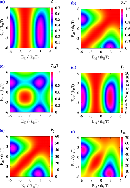
Figure 8: (Color online) Figures of merit $Z_{l}T$ (a), $Z_{t}T$ (b), and $Z_{M}T$ (c), and power factors (in unit of $10^{-4}$ W m^-1 K^-2) $P_{l}$ (d), $P_{t}$ (e), and $P_{m}$ (f) versus the QD energy $E_{\ell 0}$ and $E_{r0}$ when there is another energy level of 100 meV higher than the original one and of the same tunneling rate in each QD for both the left and the right polymer layers. $\Delta_{qd}=20$ meV and $\kappa_{p}=0.05$ W m^-1 K^-1. The temperature is $T=400$ K, and the sheet density of QDs in each polymer layer (thickness 20 nm) is $4\times 10^{12}$ cm^-2. QD tunneling linewidth is $\Gamma=30$ meV.

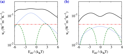
Figure 9: (Color online) Heat conductivity $\kappa_{1}$ (black full curve) and its three contributions: $\sigma S_{1}^{2}T$ (green dashed curve), $[\sigma/(e^{2}T)]\Big{[}\left\langle(E-\mu)^{2}\right\rangle_{\ell}-\left\langle E-\mu\right\rangle^{2}_{\ell}\Big{]}$ (blue dotted curve), and $\kappa_{p}$ (red chained curve) as functions of $E_{r0}=E_{\ell 0}$ for (a) with the higher level and (b) without the higher level. The higher level is 100 meV higher than the original level in each QD. $\Delta_{qd}=20$ meV and $\kappa_{p}=0.05$ W m^-1 K^-1. The temperature is $T=400$ K, and the sheet density of QDs in each polymer layer (thickness 20 nm) is $4\times 10^{12}$ cm^-2. QD tunneling linewidth is $\Gamma=30$ meV.

We calculate the figures of merit $Z_{l}T$, $Z_{t}T$, and $Z_{M}T$ and power factors $P_{l}$, $P_{t}$, and $P_{m}$ for the situation when there is another energy level of 100 meV higher than the original one in each QD for both the left and the right polymer layers. The results are plotted in Fig. 8. We assume that the tunneling rate of the higher level is the same as the lower one, i.e., $\Gamma=30$ meV. It is seen that the figures of merit as well as the power factors are all larger when the higher level is taken into account. Qualitatively, the results here is similar to those in Fig. 4 but with the center shifted toward lower energy for both $E_{\ell 0}$ and $E_{r0}$. This observation reveals that the main effect of the higher level is to enhance the electrical conductivity as well as the thermopower, which can be understood easily since a higher energy channel is introduced. However, introducing such a channel also increases the thermal conductivity which normally would reduce the figure of merit.

To clarify the underlying mechanism, we plot the thermal conductivity $\kappa_{1}$ as a function of $E_{r0}$ when $E_{\ell 0}=E_{r0}$. In Fig. 9 we plot three different contributions of $\kappa_{1}$: $\sigma S_{1}^{2}T$, $[\sigma/(e^{2}T)]\Big{[}\left\langle(E-\mu)^{2}\right\rangle_{\ell}-\left\langle E-\mu\right\rangle^{2}_{\ell}\Big{]}$, and $\kappa_{p}$. The figure of merit $Z_{l}T$ is given by $Z_{l}T=\sigma S_{1}^{2}T/(\kappa_{1}-\sigma S_{1}^{2}T)$. Indeed the thermal conductivity due to energy uncertainty $[\sigma/(e^{2}T)]\Big{[}\left\langle(E-\mu)^{2}\right\rangle_{\ell}-\left\langle E-\mu\right\rangle^{2}_{\ell}\Big{]}$ increases when higher level is introduced. However, in Fig. 9(a) (with the higher level) when $\sigma S_{1}^{2}T$ reaches its maximum value, it is very close to the other two contributions. In comparison, in Fig. 9(b) (without the higher level) when $\sigma S_{1}^{2}T$ reaches its maximum value, it is considerably smaller than the phonon heat conductivity $\kappa_{p}$. Therefore, the figure of merit $Z_{l}T$ is enhanced when the higher level is taken into account. This particular feature is because in the case without the higher level, phonon heat conductivity predominately limits the figure of merit, rather than the variance of electronic energy.

References

- (1) T. C. Harman and J. M. Honig, Thermoelectric and thermomagnetic effects and applications (McGraw-Hill, New-York, 1967); H. J. Goldsmid, Introduction to Thermoelectricity (Springer, Heidelberg, 2009).
- (2) G. J. Snyder and E. S. Toberer, Nat. Mater. 7, 105 (2008); A. Shakouri, Ann. Rev. of Mater. Res. 41, 399 (2011); T. M. Tritt, Ann. Rev. of Mater. Res. 41, 433 (2011).
- (3) G. J. Snyder and T. S. Ursell, Phys. Rev. Lett. 91, 148301 (2003).
- (4) R. Venkatasubramanian, Phys. Rev. B 61, 3091 (2000); J.-K. Yu, S. Mitrovic, D. Tham, J. Varghese, and J. R. Heath, Nat. Nanotechnol. 5, 718 (2010); N. Nakpathomkun, H. Q. Xu, and H. Linke, Phys. Rev. B 82, 235428 (2010); R. Venkatasubramanian, E. Siivola, T. Colpitts, and B. O’Quinn, Nature 413, 597 (2001).
- (5) A. I. Boukai et al., Nature 451, 168 (2008); B. Poudel et al., Science 320, 634 (2008); P. Pichanusakorn and P. Bandaru, Mater. Sci. Eng. R-Rep. 67, 19 (2010); A. J. Minnich, M. S. Dresselhaus, Z. F. Ren, and G. Chen, Energy Environ. Sci. 2, 466 (2009); C. J. Vineis, A. Shakouri, A. Majumdar, and M. G. Kanatzidis, Adv. Mater. 22, 3970 (2010); Z.-G. Chen, G. Han, L. Yang, L. Cheng, and J. Zou, Prog. Nat, Prog. Nat. Sci. 22, 535 (2012); J.-F. Li, W.-S. Liu, L.-D. Zhao, and M. Zhou, NPG Asia Mater. 2, 152 (2010).
- (6) M. S. Dresselhaus, G. Chen, M. Y. Tang, R. Yang, H. Lee, D. Wang, Z. Ren, J.-P. Fleurial, and P. Gogna, Adv. Mater. 19, 1043 (2007).
- (7) U. Sivan and Y. Imry, Phys. Rev. B 33, 551 (1986).
- (8) L. D. Hicks and M. S. Dresselhaus, Phys. Rev. B 47, 12727 (1993); ibid., 47, 16631 (1993).
- (9) G. D. Mahan and J. O. Sofo, Proc. Natl. Acad. Sci. (USA) 93, 7436 (1996).
- (10) T. E. Humphrey, R. Newbury, R. P. Taylor, and H. Linke, Phys. Rev. Lett. 89, 116801 (2002); T. E. Humphrey and H. Linke, Phys. Rev. Lett. 94, 096601 (2005).
- (11) P. Kim, L. Shi, A. Majumdar, and P. L. McEuen, Phys. Rev. Lett. 87, 215502 (2001); D. Li, Y. Wu, P. Kim, L. Shi, P. Yang, and A. Majumdar, Appl. Phys. Lett. 83, 2934 (2003); J. Hone, M. Whitney, C. Piskoti, and A. Zettl, Phys. Rev. B 59, R2514 (1999); C. Yu, L. Shi, Z. Yao, D. Li, and A. Majumdar, Nano Lett. 5, 1842 (2005).
- (12) F. Giazotto, T. T. Heikkilä, A. Luukanen, A. M. Savin, and J. P. Pekola, Rev. Mod. Phys. 78, 217 (2006).
- (13) Thermoelectric Nanomaterials, edited by K. Koumoto and T. Mori (Springer-Verlag, Berlin, 2013).
- (14) S. L. Korylyuk et al., Sov. Phys. Semicond. 7, 502 (1973); V. P. Babin et al., Sov. Phys. Semicond. 8, 478 (1974); A. Kyarad and H. Lengfellner, Appl. Phys. Lett. 89, 192103 (2006); C. Reitmaier, F. Walther, and H. Lengfellner, Appl. Phys. A 99, 717 (2010); H. J. Goldsmid, J. Electron. Mater. 40, 1254 (2011).
- (15) S. Zippilli, G. Morigi, and A. Bachtold, Phys. Rev. Lett. 102, 096804 (2009); B. Rutten, M. Esposito, and B. Cleuren, Phys. Rev. B 80, 235122 (2009).
- (16) O. Entin-Wohlman, Y. Imry, and A. Aharony, Phys. Rev. B 82, 115314 (2010).
- (17) R. Sánchez and M. Büttiker, Phys. Rev. B 83, 085428 (2011); B. Sothmann, R. Sánchez, and A. N. Jordan, arXiv:1406.5329
- (18) B. Sothmann, R. Sánchez, A. N. Jordan, and M. Büttiker, Phys. Rev. B 85, 205301 (2012).
- (19) J.-H. Jiang, O. Entin-Wohlman, and Y. Imry, Phys. Rev. B 85, 075412 (2012).
- (20) T. Ruokola and T. Ojanen, Phys. Rev. B 86, 035454 (2012).
- (21) B. Sothmann and M. Büttiker, Europhys. Lett. 99, 27001 (2012).
- (22) L. Simine and D. Segal, Phys. Chem. Chem. Phys. 14, 13820 (2012).
- (23) J.-H. Jiang, O. Entin-Wohlman, and Y. Imry, Phys. Rev. B 87, 205420 (2013).
- (24) A. N. Jordan, B. Sothmann, R. Sánchez, and M. Büttiker, Phys. Rev. B 87, 075312 (2013)
- (25) J.-H. Jiang, O. Entin-Wohlman, and Y. Imry, New J. Phys. 15, 075021 (2013).
- (26) Y. Imry, O. Entin-Wohlman, and J. H. Jiang, WO Patent 2,013,035,100.
- (27) S. Juergens, F. Haupt, M. Moskalets, and J. Splettstoesser, Phys. Rev. B 87, 245423 (2013); C. Bergenfeldt, P. Samuelsson, B. Sothmann, C. Flindt, and M. Büttiker, Phys. Rev. Lett. 112, 076803 (2014); R. Bosisio, C. Gorini, G. Fleury, and J.-L. Pichard, New J. Phys. 16, 095005 (2014); ibid., arXiv:1407.7020.
- (28) B. Sothmann, R. Sánchez, A. N. Jordan, and M. Büttiker, New J. Phys. 15, 095021 (2013).
- (29) H. L. Edwards, Q. Niu, and A. L. de Lozanne, Appl. Phys. Lett. 63, 1815 (1993); H. L. Edwards, Q. Niu, G. A. Georgakis, and A. L. de Lozanne, Phys. Rev. B 52, 5714 (1995).
- (30) J. R. Prance, C. G. Smith, J. P. Griffiths, S. J. Chorley, D. Anderson, G. A. C. Jones, I. Farrer, and D. A. Ritchie, Phys. Rev. Lett. 102, 146602 (2009).
- (31) S.-K. Park, J. Tatebayashi, and Y. Arakawa, Appl. Phys. Lett. 84, 1877 (2004); S. Tonomura and K. Yamaguchi, J. Appl. Phys. 104, 054909 (2008); M. Jo, T. Mano, Y. Sakuma, and K. Sakoda, Appl. Phys. Lett. 100, 212113 (2012).
- (32) Y. Yang, chap. 10 in Physical Properties of Polymers Handbook, edited by J. E. Mark (AIP Press, Woodbury, NY, 1996).
- (33) W. R. Algar and U. J. Krull, Langmuir 24, 5514 (2008); S. Ishii, R. Ueji, S. Nakanishi, Y. Yoshida, H. Nagata, T. Itoh, M. Ishikawa, and V. Biju, J. Photochem. Photobiol. A 183, 285 (2006).
- (34) K. Zhang, Y. Zhang, and S. Wang, Scientific Reports 3, 3448 (2013).
- (35) The polymer electronic band gap should be considerably larger than the semiconductor band gap, so that the charge carriers in the doped semiconductor regions (i.e., the cavity, source, and drain) will not diffuse into the polymer resisting layers.
- (36) R. S. Whitney, Phys. Rev. Lett. 112, 130601 (2014).
- (37) M. Gong, K. Duan, C.-F. Li, R. Magri, G. A. Narvaez, and L. He, Phys. Rev. B 77, 045326 (2008); A. D. Lad and S. Mahamuni, Phys. Rev. B 78, 125421 (2008).
- (38) H. Haug and A. P. Jauho, Quantum Kinetics in Transport and Optics of Semiconductors, (Springer, Berlin, 1996).
- (39) L. Onsager, Phys. Rev. 37, 405 (1931); 38, 2265 (1931).
- (40) Y. Demirel and S. I. Sandler, J. Phys. Chem. B 108, 31 (2004).
- (41) H. T. Odum and R. C. Pinkerton, Am. Sci. 43, 331 (1955).
- (42) J.-H. Jiang, Phys. Rev. E 90, 042126 (2014).
- (43) C. Van den Broeck, Phys. Rev. Lett. 95, 190602 (2005); M. Esposito, K. Lindenberg, and C. Van den Broeck, Phys. Rev. Lett. 102, 130602 (2009).
- (44) S. A. Gurvitz, Phys. Rev. B 57, 6602 (1998).
- (45) J. Berezovsky, O. Gywat, F. Meier, D. Battaglia, X. Peng, and D. D. Awschalom, Nat. Phys. 2, 831 (2006).
- (46) K. Koumoto et al., in CRC thermoelectric handbook: Micro to Nano, D. M, Rowe ed. (CRC press, USA, 2006).
- (47) A. Agarwal and B. Muralidharan, Appl. Phys. Lett. 105, 013104 (2014).