11email: {yutaro-s,shimbo,matsu}@is.naist.jp
22institutetext: The Institute of Statistical Mathematics, Tachikawa, Tokyo, Japan
22email: suzuki.ikumi@gmail.com
33institutetext: National Institute of Genetics, Mishima, Shizuoka, Japan
33email: kazuo.hara@gmail.com
Ridge Regression, Hubness, and Zero-Shot Learning††thanks: To be presented at ECML/PKDD 2015.
Abstract
This paper discusses the effect of hubness in zero-shot learning, when ridge regression is used to find a mapping between the example space to the label space. Contrary to the existing approach, which attempts to find a mapping from the example space to the label space, we show that mapping labels into the example space is desirable to suppress the emergence of hubs in the subsequent nearest neighbor search step. Assuming a simple data model, we prove that the proposed approach indeed reduces hubness. This was verified empirically on the tasks of bilingual lexicon extraction and image labeling: hubness was reduced with both of these tasks and the accuracy was improved accordingly.
1 Introduction
1.1 Background
In recent years, zero-shot learning (ZSL) [10, 14, 15, 22] has been an active research topic in machine learning, computer vision, and natural language processing. Many practical applications can be formulated as a ZSL task: drug discovery [15], bilingual lexicon extraction [7, 8, 20], and image labeling [2, 11, 21, 22, 25], to name a few. Cross-lingual information retrieval [28] can also be viewed as a ZSL task.
ZSL can be regarded as a type of (multi-class) classification problem, in the sense that the classifier is given a set of known example-class label pairs (training set), with the goal to predict the unknown labels of new examples (test set). However, ZSL differs from the standard classification in that the labels for the test examples are not present in the training set. In standard settings, the classifier chooses, for each test example, a label among those observed in the training set, but this is not the case in ZSL. Moreover, the number of class labels can be huge in ZSL; indeed, in bilingual lexicon extraction, labels correspond to possible translation words, which can range over entire vocabulary of the target language.
Obviously, such a task would be intractable without further assumptions. Labels are thus assumed to be embedded in a metric space (label space), and their distance (or similarity) can be measured in this space111 Throughout the paper, we assume both the example and label spaces are Euclidean. . Such a label space can be built with the help of background knowledge or external resources; in image labeling tasks, for example, labels correspond to annotation keywords, which can be readily represented as vectors in a Euclidean space, either by using corpus statistics in a standard way, or by using the more recent techniques for learning word representations, such as the continuous bag-of-words or skip-gram models [19].
After a label space is established, one natural approach would be to use a regression technique on the training set to obtain a mapping function from the example space to the label space. This function could then be used for mapping unlabeled examples into the label space, where nearest neighbor search is carried out to find the label closest to the mapped example. Finally, this label would be output as the prediction for the example.
To find the mapping function, some researchers use the standard linear ridge regression [7, 8, 20, 22], whereas others use neural networks [11, 21, 25].
In the machine learning community, meanwhile, the hubness phenomenon [23] is attracting attention as a new type of the “curse of dimensionality.” This phenomenon is concerned with nearest neighbor methods in high-dimensional space, and states that a small number of objects in the dataset, or hubs, may occur as the nearest neighbor of many objects. The emergence of these hubs will diminish the utility of nearest neighbor search, because the list of nearest neighbors often contain the same hub objects regardless of the query object for which the list is computed.
1.2 Research Objective and Contributions
In this paper, we show the interaction between the regression step in ZSL and the subsequent nearest neighbor step has a non-negligible effect on the prediction accuracy.
In ZSL, examples and labels are represented as vectors in high-dimensional space, of which the dimensionality is typically a few hundred. As demonstrated by Dinu and Baroni [8] (see also Sect. 6), when ZSL is formulated as a problem of ridge regression from examples to labels, “hub” labels emerge, which are simultaneously the nearest neighbors of many mapped examples. This has the consequence of incurring bias in the prediction, as these labels are output as the predicted labels for these examples. The presence of hubs are not necessarily disadvantageous in standard classification settings; there may be “good” hubs as well as “bad” hubs [23]. However, in typical ZSL tasks in which the label set is fine-grained and huge, hubs are nearly always harmful to the prediction accuracy.
Therefore, the objective of this study is to investigate ways to suppress hubs, and to improve the ZSL accuracy. Our contributions are as follows.
-
1.
We analyze the mechanism behind the emergence of hubs in ZSL, both with ridge regression and ordinary least squares. It is established that hubness occurs in ZSL not only because of high-dimensional space, but also because ridge regression has conventionally been used in ZSL in a way that promotes hubness. To be precise, the distributions of the mapped examples and the labels are different such that hubs are likely to emerge.
-
2.
Drawing on the above analysis, we propose using ridge regression to map labels into the space of examples. This approach is contrary to that followed in existing work on ZSL, in which examples are mapped into label space. Our proposal is therefore to reverse the mapping direction.
As shown in Sect. 6, our proposed approach outperformed the existing approach in an empirical evaluation using both synthetic and real data.
-
3.
In terms of contributions to the research on hubness, this paper is the first to provide in-depth analysis of the situation in which the query and data follow different distributions, and to show that the variance of data matters to hubness. In particular, in Sect. 3, we provide a proposition in which the degree of bias present in the data, which causes hub formation, is expressed as a function of the data variance. In Sect 4, this proposition serves as the main tool for analyzing hubness in ZSL.
2 Zero-Shot Learning as a Regression Problem
Let be a set of examples, and be a set of class labels. In ZSL, not only examples but also labels are assumed to be vectors. For this reason, examples are sometimes referred to as source objects, and labels as target objects. In the subsequent sections of this paper, we mostly follow this terminology when referring to the members of and .
Let and . These spaces, and , are called source space and target space, respectively. Although can be the entire space , is usually a finite set of points in , even though its size may be enormous in some problems.
Let be the training examples (training source objects), and be their labels (training target objects); i.e., the class label of example is , for each . In a standard classification setting, the labels in the training set are equal to the entire set of labels; i.e., . In contrast, this assumption is not made in ZSL, and is a strict subset of . Moreover, it is assumed that the true class labels of test examples do not belong to ; i.e., they belong to .
In such a situation, it is difficult to find a function that maps directly to a label in . Therefore, a popular (and also natural) approach is to learn a projection , which can be done with a regression technique. With a projection function at hand, the label of a new source object is predicted to be the one closest to the mapped point in the target space. The prediction function is thus given by
After a source object is projected to , the task is reduced to that of nearest neighbor search in the target space.
3 Hubness Phenomenon and the Variance of Data
The utility of nearest neighbor search would be significantly reduced if the same objects were to appear consistently as the search result, irrespective of the query. Radovanović et al. [23] showed that such objects, termed hubs, indeed occur in high-dimensional space. Although this phenomenon may seem counter-intuitive, hubness is observed in a variety of real datasets and distance/similarity measures used in combination [23, 24, 26].
The aim of this study is to analyze the hubness phenomenon in ZSL, which involves nearest neighbor search in high-dimensional space as the last step. However, as a tool for analyzing ZSL, the existing theory on hubness [23] is inadequate, as it was mainly developed for comparing the emergence of hubness in spaces of different dimensionalities.
In the analysis of ZSL in Sect. 4.2, we aim to compare two distributions in the same space, but which differ in terms of variance. To this end, we first present a proposition below, which is similar in spirit to the main theorem of Radovanović et al. [23, Theorem 1], but which distinguishes the query and data distributions, and also expresses the expected difference between the squared distances from queries to database objects in terms of their variance.
The proposition is concerned with nearest neighbor search, in which is a query, and and are two objects in a dataset. In the context of ZSL as formulated in Sect. 2, represents the image of a source object in the target space (through the learned regression function ), and and are target objects (labels) lying at different distances from the origin. We are interested in which of and are more likely to be closer to , when is sampled from a distribution with zero mean.
Let and denote the expectation and variance, respectively, and let be a multivariate normal distribution with mean and covariance matrix .
Proposition 1
Let be a -dimensional random vector, with components () sampled i.i.d. from a normal distribution with zero mean and variance ; i.e., , where . Further let be the standard deviation of the squared norm .
Consider two fixed samples and of random vector , such that the squared norms of and are apart. In other words,
Let be a point sampled from a distribution with zero mean. Then, the expected difference between the squared distances from and to , i.e.,
| (1) |
is given by
| (2) |
Proof
For , the distance between a point and is given by
and its expected value is
since by assumption. Substituting this equality in (1) yields
| (3) |
Now, it is well known that if a -dimensional random vector follows the multivariate standard normal distribution , then its squared norm follows the chi-squared distribution with degrees of freedom, and its variance is . Since , the variance of the squared norm is
| (4) |
Note that in Proposition 1, the standard deviation is used as a yardstick of measurement to allow for comparison of “similarly” located object pairs across different distributions; two object pairs in different distributions are regarded as similar if objects in each pair are apart as measured by the for the respective distributions, but has an equal factor . This technique is due to Radovanović et al. [23].
Now, represents the expected difference between the squared distances from to and . Equation (2) shows that increases with , the factor quantifying the amount of difference . This suggests that a query object sampled from is more likely to be closer to object than to , if ; i.e., is closer to the origin than is. Because this holds for any pair of objects and in the dataset, we can conclude that the objects closest to the origin in the dataset tend to be hubs.
Equation (2) also states the relationship between and the component variance of distribution , by which the following is implied: For a fixed query distribution , if we have two distributions for , and with , it is preferable to choose , i.e., the distribution with a smaller , when attempting to reduce hubness. Indeed, assuming the independence of and , we can show that the influence of relative to the expected squared distance from to (which is also subject to whether or ), is weaker for than for , i.e.,
where we wrote explicitly as a function of , , and .
4 Hubness in Regression-Based Zero-Shot Learning
In this section, we analyze the emergence of hubs in the nearest neighbor step of ZSL. Through the analysis, it is shown that hubs are promoted by the use of ridge regression in the existing formulation of ZSL, i.e., mapping source objects (examples) into the target (label) space.
As a solution, we propose using ridge regression in a direction opposite to that in existing work. That is, we project target objects in the space of source objects, and carry out nearest neighbor search in the source space. Our argument for this approach consists of three steps.
-
1.
We first show in Sect. 4.1 that, with ridge regression (and ordinary least squares as well), mapped observation data tend to lie closer to the origin than the target responses do. Because the existing work formulates ZSL as a regression problem that projects source objects into the target space, this means that the norm of the projected source objects tends to be smaller than that of target objects.
-
2.
By combining the above result with the discussion of Sect. 3, we then argue that placing source objects closer to the origin is not ideal from the perspective of reducing hubness. On the contrary, placing target objects closer to the origin, as attained with the proposed approach, is more desirable (Sect. 4.2).
-
3.
In Sect. 4.3, we present a simple additional argument against placing source objects closer to the origin; if the data is unimodal, such a configuration increases the possibility of another target object falling closer to the source object. This argument diverges from the discussion on hubness, but again justifies the proposed approach.
4.1 Shrinkage of Projected Objects
We first prove that ridge regression tends to map observation data closer to the origin of the space. This tendency may be easily observed in ridge regression, for which the penalty term shrinks the estimated coefficients towards zero. However, the above tendency is also inherent in ordinary least squares.
Let and respectively denote the Frobenius norm and the 2-norm of matrices.
Proposition 2
Let be the solution for ridge regression with an observation matrix and a response matrix ; i.e.,
| (5) |
where is a hyperparameter. Then, we have .
Proof (Sketch)
It is well known that . Thus we have
| (6) |
Let be the largest singular value of . It can be shown that
Substituting this inequality in (6) establishes the proposition. ∎
Recall that if the data is centered, the matrix 2-norm can be interpreted as an indicator of the variance of data along its principal axis. Proposition 2 thus indicates that the variance along the principal axis of the mapped observations tends to be smaller than that of responses .
Furthermore, this tendency even persists in the ordinary least squares with no penalty term (i.e., ), since still holds in this case; note that is an orthogonal projection and its 2-norm is , but the inequality in (6) holds regardless. This tendency therefore cannot be completely eliminated by simply decreasing the ridge parameter towards zero.
In existing work on ZSL, represents the (training) source objects , to be mapped into the space of target objects (by projection matrix ); and is the matrix of labels for the training objects, i.e., . Although Proposition 2 is thus only concerned with the training set, it suggests that the source objects at the time of testing, which are not in , are also likely to be mapped closer to the origin of the target space than many of the target objects in .
4.2 Influence of Shrinkage on Nearest Neighbor Search
We learned in Sect. 4.1 that ridge regression (and ordinary least squares) shrink the mapped observation data towards the origin of the space, relative to the response. Thus, in existing work on ZSL in which source objects are projected to the space of target objects , the norm of the mapped source objects is likely to be smaller than that of the target objects.
The proposed approach, which was described in the beginning of Sect. 4, follows the opposite direction: target objects are projected to the space of source objects . Thus, in this case, the norm of the mapped target objects is expected to be smaller than that of the source objects.
The question now is which of these configurations is preferable for the subsequent nearest neighbor step, and we provide an answer under the following assumptions: (i) The source space and the target space are of equal dimensions; (ii) the source and target objects are isotropically normally distributed and independent; and (iii) the projected data is also isotropically normally distributed, except that the variance has shrunk.
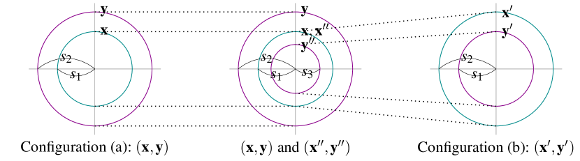
Let and be two multivariate normal distributions, with . We compare two configurations of source object and target objects : (a) the one in which and , and (b) the one in which and on the other hand; here, the primes in (b) were added to distinguish variables in two configurations.
These two configurations are intended to model situations in (a) existing work and (b) our proposal. In configuration (a), is shorter in expectation than , and therefore this approximates the situation that arises from existing work. Configuration (b) represents the opposite situation, and corresponds to our proposal in which is the projected vector and thus is shorter in expectation than .
Now, we aim to verify whether the two configurations differ in terms of the likeliness of hubs emerging, using Proposition 1. First, we scale the entire space of configuration (b) by , or equivalently, we consider transformation of the variables by and . Note that because the two variables are scaled equally, this change of variables preserves the nearest neighbor relations among the samples. See Fig. 1 for an illustration of the relationship among , , , , , and .
Let and be the components of and , respectively, and let and be those for and . Then we have
Thus, follows , and follows . Since both in configuration (a) and above follow the same distribution, it now becomes possible to compare the properties of and in light of the discussion at the end of Sect. 3: In order to reduce hubness, the distribution with a smaller variance is preferred to the one with a larger variance, for a fixed distribution of source (or equivalently, ).
It follows that is preferable to , because the former has a smaller variance. As mentioned above, the nearest neighbor relation between the scaled variables, against (or equivalently ), is identical to against in configuration (b). Therefore, we conclude that configuration (b) is preferable to configuration (a), in the sense that the former is more likely to suppress hubs.
Finally, recall that the preferred configuration (b) models the situation of our proposed approach, which is to map target objects in the space of source objects.
4.3 Additional Argument for Placing Target Objects Closer to the Origin
By assuming a unimodal data distribution of which the probability density function (pdf) is decreasing in , we are able to present the following proposition which also advocates placing the source objects outside the target objects, and not the other way around.
Proposition 3 is concerned with the placement of a source object at a fixed distance from its target object , for which we have two alternatives and , located at different distances from the origin of the space.
Proposition 3
Consider a finite set of objects (i.e., points) in a Euclidean space, sampled i.i.d. from a distribution whose pdf is a decreasing function of . Let be an object in the set, and let . Further let and be two objects at a distance apart from . If , then the probability that is the closest object in to is greater than that of .
Proof (Sketch)
For , if another object in appears within distance of , then is not the nearest neighbor of . Thus, we aim to prove that this probability for is smaller than that for . Since objects in are sampled i.i.d, it suffices to prove
| (7) |
where () denote the balls centered at with radius . However, (7) obviously holds because the balls and have the same radii, is a decreasing function of , and . See Figure 2 for an illustration with a bivariate standard normal distribution in two-dimensional space. ∎

In the context of existing work on ZSL, which uses ridge regression to map source objects in the space of target objects, can be regarded as a mapped source object, and as its target object. Proposition 3 implies that if we want to make a source object the nearest neighbor of a target object , it should rather be placed farther than from the origin, but this idea is not present in the objective function (5) for ridge regression; the first term of the objective allocates the same amount of penalty for and , as they are equally distant from the target . On the contrary, the ridge regression actually promotes placement of the mapped source object closer to the origin, as stated in Proposition 2.
4.4 Summary of the Proposed Approach
Drawing on the analysis presented in Sections 4.1–4.3, we propose performing regression that maps target objects in the space of source objects, and carry out nearest neighbor search in the source space. This opposes the approach followed in existing work on regression-based ZSL [7, 8, 16, 20, 22], which maps source objects into the space of target objects.
In the proposed approach, matrix in Proposition 2 represents the source objects , and represents the target objects . Therefore, means , i.e., the mapped target objects tend to be placed closer than the corresponding source objects to the origin.
Admittedly, the above argument for our proposal relies on strong assumptions on data distributions (such as normality), which do not apply to real data. However, the effectiveness of our proposal is verified empirically in Sect. 6 by using real data.
5 Related Work
The first use of ridge regression in ZSL can be found in the work of Palatucci et al. [22]. Ridge regression has since been one of the standard approaches to ZSL, especially for natural language processing tasks: phrase generation [7] and bilingual lexicon extraction [7, 8, 20]. More recently, neural networks have been used for learning non-linear mapping [11, 25]. All of the regression-based methods listed above, including those based on neural networks, map source objects into the target space.
ZSL can also be formulated as a problem of canonical correlation analysis (CCA). Hardoon et. al. [12] used CCA and kernelized CCA for image labeling. Lazaridou et. al. [16] compared ridge regression, CCA, singular value decomposition, and neural networks in image labeling. In our experiments (Sect. 6), we use CCA as one of the baseline methods for comparison.
Dinu and Baroni [8] reported the hubness phenomenon in ZSL. They proposed two reweighting techniques to reduce hubness in ZSL, which are applicable to cosine similarity. Tomašev et al. [27] proposed hubness-based instance weighting schemes for CCA. These schemes were applied to classification problems in which multiple instances (vectors) in the target space have the same class label. This setting is different from the one assumed in this paper (see Sect. 2), i.e., we assume that a class label is represented by a single target vector.222 Perhaps because of this difference, the method in [27] did not perform well in our experiment, and we do not report its result in Sect. 6.
Structured output learning [4] addresses a problem setting similar to ZSL, except that the target objects typically have complex structure, and thus the cost of embedding objects in a vector space is prohibitive. Kernel dependency estimation [29] is an approach that uses kernel PCA and regression to avoid this issue. In this context, nearest neighbor search in the target space reduces to the pre-image problem [18] in the implicit space induced by kernels.
6 Experiments
We evaluated the proposed approach with both synthetic and real datasets. In particular, it was applied to two real ZSL tasks: bilingual lexicon extraction and image labeling.
The main objective of the following experiments is to verify whether our proposed approach is capable of suppressing hub formation and outperforming the existing approach, as claimed in Sect. 4.
6.1 Experimental Setups
6.1.1 Compared Methods.
The following methods were compared.
We calibrated the hyperparameters, i.e., the regularization parameter in ridge regression and the dimensionality of common feature space in CCA, by cross validation on the training set.
After ridge regression or CCA is applied, both X and Y (or their images) are located in the same space, wherein we find the closest target object for a given source object as measured by the Euclidean distance. In addition to the Euclidean distance, we also tested the non-iterative contextual dissimilarity measure (NICDM) [13] in combination with and CCA. NICDM adjusts the Euclidean distance to make the neighborhood relations more symmetrical, and is known to effectively reduce hubness in non-ZSL context [24].
All data were centered before application of regression and CCA, as usual with these methods.
6.1.2 Evaluation Criteria.
The compared methods were evaluated in two respects: (i) the correctness of their prediction, and (ii) the degree of hubness in nearest neighbor search.
Measures of Prediction Correctness.
In all our experiments, ZSL was formulated as a ranking task; given a source object, all the target objects were ranked by their likelihood for the source object. As the main evaluation criterion, we used the mean average precision (MAP) [17], which is one of the standard performance metrics for ranking methods. Note that the synthetic and the image labeling experiments are the single-label problems for which MAP is equal to the mean reciprocal rank [17]. We also report the top- accuracy333 In image labeling (only), we report the top-1 accuracy () macro-averaged over classes, to allow direct comparison with published results. Note also that with a larger would not be an informative metric for the image labeling task, which only has 10 test labels. () for and , which is the percentage of source objects for which the correct target objects are present in their nearest neighbors.
Measure of Hubness.
To measure the degree of hubness, we used the skewness of the (empirical) distribution, following the approach in the literature [23, 24, 26, 27]. The distribution is the distribution of the number of times each target object is found in the top of the ranking for source objects, and its skewness is defined as follows:
where is the total number of test objects in , is the number of times the th target object is in the top- closest target objects of the source objects. A large skewness value indicates the existence of target objects that frequently appear in the -nearest neighbor lists of source objects; i.e., the emergence of hubs.
6.2 Task Descriptions and Datasets
We tested our method on the following ZSL tasks.
6.2.1 Synthetic Task.
To simulate a ZSL task, we need to generate object pairs across two spaces in a way that the configuration of objects is to some extent preserved across the spaces, but is not exactly identical. To this end, we first generated 3000-dimensional (column) vectors for , whose coordinates were generated from an i.i.d. univariate standard normal distribution. Vectors were treated as latent variables, in the sense that they were not directly observable, but only their images and in two different features spaces were. These images were obtained via different random projections, i.e., and , where are random matrices whose elements were sampled from the uniform distribution over . Because random projections preserve the length and the angle of vectors in the original space with high probability [5, 6], the configuration of the projected objects is expected to be similar (but different) across the two spaces.
Finally, we randomly divided object pairs into the training set (8000 pairs) and the test set (remaining 2000 pairs).
6.2.2 Bilingual Lexicon Extraction.
Our first real ZSL task is bilingual lexicon extraction [7, 8, 20], formulated as a ranking task: Given a word in the source language, the goal is to rank its gold translation (the one listed in an existing bilingual lexicon as the translation of the source word) higher than other non-translation candidate words.
In this experiment, we evaluated the performance in the tasks of finding the English translations of words in the following source languages: Czech (cs), German (de), French (fr), Russian (ru), Japanese (ja), and Hindi (hi). Thus, in our setting, each of these six languages was used as alternately, whereas English was the target language throughout.444 We also conducted experiments with English as and other languages as . The results are not presented here due to lack of space, but the same trend was observed.
Following related work [7, 8, 20], we trained a CBOW model [19] on the pre-processed Wikipedia corpus distributed by the Polyglot project555https://sites.google.com/site/rmyeid/projects/polyglot (see [3] for corpus statistics), using the word2vec666https://code.google.com/p/word2vec/ tool. The window size parameter of word2vec was set to 10, with the dimensionality of feature vectors set to 500.
To learn the projection function and measure the accuracy in the test set, we used the bilingual dictionaries777http://hlt.sztaki.hu/resources/dict/bylangpair/wiktionary_2013july/ of Ács et al. [1] as the gold translation pairs. These gold pairs were randomly split into the training set (80% of the whole pairs) and the test set (20%). We repeated experiments on four different random splits, for which we report the average performance.
6.2.3 Image Labeling.
The second real task is image labeling, i.e., the task of finding a suitable word label for a given image. Thus, source objects are the images and target objects are the word labels.
We used the Animal with Attributes (AwA) dataset888 http://attributes.kyb.tuebingen.mpg.de/ , which consists of 30,475 images of 50 animal classes. For image representation, we used the DeCAF features [9], which are the 4096-dimensional vectors constructed with convolutional neural networks (CNNs). DeCAF is also available from the AwA website. To save computational cost, we used random projection to reduce the dimensionality of DeCAF features to 500.
As with the bilingual lexicon extraction experiment, label features (word representations) were constructed with word2vec, but this time they were trained on the English version of Wikipedia (as of March 4, 2015) to cover all AwA labels. Except for the corpus, we used the same word2vec parameters as with bilingual lexicon extraction.
We respected the standard zero-shot setup on AwA provided with the dataset; i.e., the training set contained 40 labels, and test set contained the other 10 labels.
6.3 Experimental Results
| method | MAP | ||||
|---|---|---|---|---|---|
| 21.5 | 13.8 | 36.3 | 24.19 | 12.75 | |
| + NICDM | 58.2 | 47.6 | 78.4 | 13.71 | 7.94 |
| (proposed) | 91.7 | 87.6 | 98.3 | 0.46 | 1.18 |
| CCA | 78.9 | 71.6 | 91.7 | 12.0 | 7.56 |
| CCA + NICDM | 87.6 | 82.3 | 96.5 | 0.96 | 2.58 |
| method | cs | de | fr | ru | ja | hi |
|---|---|---|---|---|---|---|
| 1.7 | 1.0 | 0.7 | 0.5 | 0.9 | 5.3 | |
| + NICDM | 11.3 | 7.1 | 5.9 | 3.8 | 10.2 | 21.4 |
| (proposed) | 40.8 | 30.3 | 46.5 | 31.1 | 42.0 | 40.6 |
| CCA | 24.0 | 18.1 | 33.7 | 21.2 | 27.3 | 11.8 |
| CCA + NICDM | 30.1 | 23.4 | 39.7 | 26.7 | 35.3 | 19.3 |
| cs | de | fr | ru | ja | hi | |||||||
|---|---|---|---|---|---|---|---|---|---|---|---|---|
| method | ||||||||||||
| 0.7 | 2.8 | 0.4 | 1.6 | 0.3 | 1.2 | 0.2 | 0.8 | 0.2 | 1.3 | 2.9 | 8.2 | |
| + NICDM | 7.2 | 17.9 | 4.3 | 11.4 | 3.5 | 9.8 | 2.1 | 6.3 | 6.1 | 16.8 | 14.4 | 32.6 |
| (proposed) | 31.5 | 54.5 | 21.6 | 43.0 | 36.6 | 58.6 | 21.9 | 43.6 | 31.9 | 56.3 | 31.1 | 55.4 |
| CCA | 17.9 | 32.7 | 12.9 | 25.2 | 27.0 | 41.7 | 15.2 | 28.8 | 20.2 | 37.3 | 7.4 | 18.9 |
| CCA + NICDM | 21.9 | 42.3 | 16.1 | 33.9 | 31.1 | 50.1 | 18.7 | 37.0 | 25.9 | 48.8 | 12.4 | 30.7 |
| cs | de | fr | ru | ja | hi | |||||||
|---|---|---|---|---|---|---|---|---|---|---|---|---|
| method | ||||||||||||
| 50.29 | 23.84 | 43.00 | 24.37 | 67.79 | 35.83 | 95.05 | 35.36 | 62.12 | 22.78 | 23.75 | 10.84 | |
| + NICDM | 41.56 | 20.38 | 39.32 | 20.82 | 57.18 | 25.97 | 89.08 | 30.70 | 57.57 | 21.62 | 20.33 | 9.21 |
| (proposed) | 11.91 | 10.74 | 12.49 | 11.94 | 2.56 | 2.77 | 4.28 | 4.18 | 5.15 | 6.76 | 10.45 | 6.14 |
| CCA | 28.00 | 18.67 | 36.66 | 18.98 | 30.18 | 15.95 | 51.92 | 21.60 | 37.73 | 18.27 | 22.31 | 8.95 |
| CCA + NICDM | 25.00 | 17.13 | 32.94 | 17.65 | 25.20 | 14.65 | 42.61 | 20.72 | 34.66 | 13.16 | 22.00 | 8.46 |
| method | MAP | ||
|---|---|---|---|
| 46.0 | 22.6 | 2.61 | |
| + NICDM | 54.2 | 34.5 | 2.17 |
| (proposed) | 62.5 | 41.3 | 0.08 |
| CCA | 26.1 | 9.2 | 2.00 |
| CCA + NICDM | 26.9 | 9.3 | 2.42 |
Table 1 shows the experimental results. The trends are fairly clear: The proposed approach, , outperformed other methods in both MAP and , over all tasks. and CCA combined with NICDM performed better than those with Euclidean distances, although they still lagged behind the proposed method even with NICDM.
The skewness achieved by was lower (i.e., better) than that of compared methods, meaning that it effectively suppressed the emergence of hub labels. In contrast, produced a high skewness which was in line with its poor prediction accuracy. These results support the expectation we expressed in the discussion in Sect. 4.
The results presented in the tables show that the degree of hubness () for all tested methods inversely correlates with the correctness of the output rankings, which strongly suggests that hubness is one major factor affecting the prediction accuracy.
For the AwA image dataset, Akata et. al. [2, the fourth row (CNN) and second column () of Table 2] reported a 39.7% score, using image representations trained with CNNs, and 100-dimensional word representations trained with word2vec. For comparison, our proposed approach, , was evaluated in a similar setting: We used the DeCAF features (which were also trained with CNNs) without random projection as the image representation, and 100-dimensional word2vec word vectors. In this setup, achieved a 40.0% score. Although the experimental setups are not exactly identical and thus the results are not directly comparable, this suggests that even linear ridge regression can potentially perform as well as more recent methods, such as Akata et al.’s, simply by exchanging the observation and response variables.
7 Conclusion
This paper has presented our formulation of ZSL as a regression problem of finding a mapping from the target space to the source space, which opposes the way in which regression has been applied to ZSL to date. Assuming a simple model in which data follows a multivariate normal distribution, we provided an explanation as to why the proposed direction is preferable, in terms of the emergence of hubs in the subsequent nearest neighbor search step. The experimental results showed that the proposed approach outperforms the existing regression-based and CCA-based approaches to ZSL.
Future research topics include: (i) extending the analysis of Sect. 4 to cover multi-modal data distributions, or other similarity/distance measures such as cosine; (ii) investigating the influence of mapping directions in other regression-based ZSL methods, including neural networks; and (iii) investigating the emergence of hubs in CCA.
Acknowledgments.
We thank anonymous reviewers for their valuable comments and suggestions. MS was supported by JSPS Kakenhi Grant no. 15H02749.
References
- [1] Ács, J., Pajkossy, K., Kornai, A.: Building basic vocabulary across 40 languages. In: Proceedings of the 6th Workshop on Building and Using Comparable Corpora. pp. 52–58 (2013)
- [2] Akata, Z., Lee, H., Schiele, B.: Zero-shot learning with structured embeddings. arXiv preprint arXiv:1409.8403v1 (2014)
- [3] Al-Rfou, R., Perozzi, B., Skiena, S.: Polyglot: Distributed word representations for multilingual NLP. In: CoNLL ’13. pp. 183–192 (2013)
- [4] Bakir, G., Hofmann, T., Schölkopf, B., Smola, A.J., Taskar, B., Vishwanathan, S.V.N. (eds.): Predicting Structured Data. MIT press (2007)
- [5] Bingham, E., Mannila, H.: Random projection in dimensionality reduction: Applications to image and text data. In: KDD ’01. pp. 245–250 (2001)
- [6] Dasgupta, S.: Experiments with random projection. In: UAI ’00. pp. 143–151 (2000)
- [7] Dinu, G., Baroni, M.: How to make words with vectors: Phrase generation in distributional semantics. In: ACL ’14. pp. 624–633 (2014)
- [8] Dinu, G., Baroni, M.: Improving zero-shot learning by mitigating the hubness problem. In: Workshop at ICLR ’15 (2015)
- [9] Donahue, J., Jia, Y., Vinyals, O., Hoffman, J., Zhang, N., Tzeng, E., Darrell, T.: DeCAF: A deep convolutional activation feature for generic visual recognition. arXiv preprint arXiv:1310.1531 (2013)
- [10] Farhadi, A., Endres, I., Hoiem, D., Forsyth, D.: Describing objects by their attributes. In: CVPR ’09. pp. 1778–1785 (2009)
- [11] Frome, A., Corrado, G.S., Shlens, J., Bengio, S., Dean, J., Ronzato, M., Mikolov, T.: Devise: A deep visual-semantic embedding model. In: NIPS ’13. pp. 2121–2129 (2013)
- [12] Hardoon, D.R., Szedmak, S., Shawe-Taylor, J.: Canonical correlation analysis: An overview with application to learning methods. Neural Computation 16, 2639–2664 (2004)
- [13] Jegou, H., Harzallah, H., Schmid, C.: A contextual dissimilarity measure for accurate and efficient image search. In: CVPR ’07. pp. 1–8 (2007)
- [14] Lampert, C.H., Nickisch, H., Harmeling, S.: Learning to detect unseen object classes by between-class attribute transfer. In: CVPR ’09. pp. 951–958 (2009)
- [15] Larochelle, H., Erhan, D., Bengio, Y.: Zero-data learning of new tasks. In: AAAI ’08. pp. 646–651 (2008)
- [16] Lazaridou, A., Bruni, E., Baroni, M.: Is this a wampimuk? Cross-modal mapping between distributional semantics and the visual world. In: ACL ’14. pp. 1403–1414 (2014)
- [17] Manning, C.D., Raghavan, P., Schütze, H.: Introduction to Information Retrieval. Cambridge University Press (2008)
- [18] Mika, S., Schölkopf, B., Smola, A., Müller, K.R., Scholz, M., Rätsch, G.: Kernel PCA and de-noising in feature space. In: NIPS ’98. pp. 536–542 (1998)
- [19] Mikolov, T., Chen, K., Corrado, G., Dean, J.: Efficient estimation of word representations in vector space. In: Workshop at ICLR ’13 (2013)
- [20] Mikolov, T., Le, Q.V., Sutskever, I.: Exploiting similarities among languages for machine translation. arXiv preprint arXiv:1309.4168 (2013)
- [21] Norouzi, M., Mikolov, T., Bengio, S., Singer, Y., Shlens, J., Frome, A., Corrado, G.S., Dean, J.: Zero-shot learning by convex combination of semantic embeddings. In: ICLR ’14 (2014)
- [22] Palatucci, M., Pomerleau, D., Hinton, G., Mitchell, T.M.: Zero-shot learning with semantic output codes. In: NIPS ’09. pp. 1410–1418 (2009)
- [23] Radovanović, M., Nanopoulos, A., Ivanović, M.: Hubs in space: Popular nearest neighbors in high-dimensional data. Journal of Machine Learning Research 11, 2487–2531 (2010)
- [24] Schnitzer, D., Flexer, A., Schedl, M., Widmer, G.: Local and global scaling reduce hubs in space. Journal of Machine Learning Research 13, 2871–2902 (2012)
- [25] Socher, R., Ganjoo, M., Manning, C.D., Ng, A.Y.: Zero-shot learning through cross-modal transfer. In: NIPS ’13. pp. 935–943 (2013)
- [26] Suzuki, I., Hara, K., Shimbo, M., Saerens, M., Fukumizu, K.: Centering similarity measures to reduce hubs. In: EMNLP ’13. pp. 613–623 (2013)
- [27] Tomašev, N., Rupnik, J., Mladenić, D.: The role of hubs in cross-lingual supervised document retrieval. In: PAKDD ’13. pp. 185–196 (2013)
- [28] Vinokourov, A., Shawe-Taylor, J., Cristianini, N.: Inferring a semantic representation of text via cross-language correlation analysis. In: NIPS ’02. pp. 1473–1480 (2002)
- [29] Weston, J., Chapelle, O., Vapnik, V., Elisseeff, A., Schölkopf, B.: Kernel dependency estimation. In: NIPS ’02. pp. 873–880 (2002)