A giant ring-like structure at $0.78<z<0.86$ displayed by GRBs

Abstract

According to the cosmological principle, Universal large-scale structure is homogeneous and isotropic. The observable Universe, however, shows complex structures even on very large scales. The recent discoveries of structures significantly exceeding the transition scale of 370 Mpc pose a challenge to the cosmological principle.

We report here the discovery of the largest regular formation in the observable Universe; a ring with a diameter of 1720 Mpc, displayed by 9 gamma ray bursts (GRBs), exceeding by a factor of five the transition scale to the homogeneous and isotropic distribution. The ring has a major diameter of $43^{o}$ and a minor diameter of $30^{o}$ at a distance of 2770 Mpc in the $0.78<z<0.86$ redshift range, with a probability of $2\times 10^{-6}$ of being the result of a random fluctuation in the GRB count rate.

Evidence suggests that this feature is the projection of a shell onto the plane of the sky. Voids and string-like formations are common outcomes of large-scale structure. However, these structures have maximum sizes of 150 Mpc, which are an order of magnitude smaller than the observed GRB ring diameter. Evidence in support of the shell interpretation requires that temporal information of the transient GRBs be included in the analysis.

This ring-shaped feature is large enough to contradict the cosmological principle. The physical mechanism responsible for causing it is unknown.

1 Introduction

Quasars are well-suited for mapping out the large-scale distribution of matter in the Universe, due to their very high luminosities and preferentially large redshifts. Quasars are associated by groups and poor clusters of galaxies (Heinämäki et al., 2005; Lietzen et al., 2009) and can be observed even when the underlying galaxies are faint and difficult to detect. When quasars cluster, they identify considerable amounts of underlying matter, such that quasar clusters have been used to detect matter clustered on very large scales. Some of this matter is clustered on scales equal to or exceeding that of the Sloan Great Wall (Gott et al., 2005).

A number of large quasar groups (LQG) have been identified in recent years; each one mapping out large amounts of much fainter matter. After Webster (1982) found a group of four quasars at $z=0.37$ with a size of about 100 Mpc, having a low probability of being a chance alignment, Komberg, Kravtsov & Lukash (1994) identified strong clustering in the quasar distribution at scales less than $20\,h^{-1}$ Mpc, and defined LQGs using a well-known cluster analysis technique. Subsequently, Komberg, Kravtsov & Lukash (1996) identified additional LQGs, and Komberg & Lukash (1998) reported a new finding of eleven LQGs based on systematic cluster analysis. The sizes of these clusters ranged from 70 to 160 $h^{-1}$ Mpc. Newman et al. (1998a, b) later discovered a $~{}150\,h^{-1}$ Mpc group of 13 quasars at median redshift $z\cong 1.51$. Williger et al. (2002) mapped 18 quasars spanning $\approx 5^{\circ}\times 2.5^{\circ}$ on the sky, with a quasar spatial overdensity $6-10$ times greater than the mean. Haberzettl et al. (2009) investigated two sheet-like structures of galaxies at $z=0.8$ and $1.3$ spanning $150\,h^{-1}$ comoving Mpc embedded in LQGs extending over at least $200\,h^{-1}$ Mpc. Haines, Campusano & Clowes (2004) reported the finding of two large-scale structures of galaxies in a $40\times 35$ arcmin² field embedded in a $25^{\circ 2}$ area containing two 100 Mpc-scale structures of quasars. As the identified scales of quasar clusters became larger, Clowes et al. (2012) found two relatively close LQGs at $z\sim 1.2$. The characteristic sizes of these two LQGs, $\approx 350-400$ Mpc, and appear to be only marginally consistent with the scale of homogeneity in the concordance cosmology. Recently, Clowes et al. (2013) uncovered the Huge-LQG with a long dimension of $\approx 1240$ Mpc ($1240\times 640\times 370$ Mpc). Until recently, this was the largest known structure in the Universe. Using a friend of friend (FoF) algorithm Einasto et al. (2014) found that the linking length $l=70\,h^{-1}Mpc$ three systems from their QSR catalogue coincide with the LQGs from Clowes et al. (2012, 2013).

Horváth, Hakkila & Bagoly (2013, 2014) announced the discovery of a larger Universal structure than the Huge-LQG by analyzing the spatial distribution of gamma-ray bursts (GRBs). The 3000 Mpc size of this structure exceeds the size of the Sloan Great Wall by a factor of about six; This is currently the largest known universal structure.

Unlike quasars, GRBs are short-lived cosmic transients spanning milliseconds to hundreds of seconds (see the review paper by Mészáros, 2006). Due to their immense luminosities, GRBs can be observed at very large cosmological distances. Their hosts are typically metal poor galaxies of intermediate mass (Savaglio, Glazebrook & Le Borgne, 2009; Castro Cerón et al., 2010; Levesque et al., 2010), rather than the massive galaxies in which quasars are generally found. Both quasars and GRBs should map the underlying distribution of universal matter, although the details of their spatial distributions are not necessarily identical. Although the number of known GRBs for which distances have been accurately measured is significantly fewer than the number of known quasars, the surveying techniques used to identify these objects are more homogeneous and better-suited for studying structures of large angular size than are quasars.

The existence of an object with a size of several gigaparsecs introduces questions concerning the homogenous and isotropic nature of cosmological models. The great importance of this question necessitates further independent study into the use of GRBs for mapping large-scale universal structures. Our analysis considers the space distribution of a GRB sample having known redshifts for the presence of large-scale anisotropies. The sample we use for this study is available at http://www.astro.caltech.edu/grbox/grbox.php. As of October 2013, the redshifts of 361 GRBs have been determined.

2 Distribution of GRBs in $\{r,\theta,\varphi\}$ space

According to the cosmological principle ($CP$), Universal large-scale structure is homogeneous and isotropic (Ellis, 1975). The WMAP and Planck experiments have revealed that the Big Bang had these properties in its early expansion phase. The observable Universe, however, shows complex structures even on very large scales. The problem is to find a limiting scale at which the $CP$ is valid.

A number of well-known studies have attempted to find the largest scale on which $CP$ is valid. According to Einasto & Gramann (1993) the available data suggested values $r(t)=130\pm 10\,h^{-1}$. Yahata et al. (2005) reported on the first result from the clustering analysis of SDSS quasars: the bump in the power spectrum due to the baryon density was not clearly visible, and they concluded that the galaxy distribution was homogeneous on scales larger than $60-70\,h^{-1}$ Mpc. Tegmark et al. (2006) using luminous red galaxies (LRGs) in the Sloan Digital Sky Survey (SDSS) improved the evidence for spatial flatness ($\Omega_{tot}=1$). Liivamägi, Tempel & Saar (2012) have constructed a set of supercluster catalogues for the galaxies from the SDSS survey main and LRG flux-limited samples. Bagla, Yadav & Seshadri (2008) showed that in the concordance model, the fractal dimension makes a rapid transition to values close to 3 at scales between 40 and 100 Mpc. Sarkar et al. (2009) found the galaxy distribution to be homogeneous at length-scales greater than $70\,h^{-1}$ Mpc, and Yadav, Bagla & Khandai (2010) estimated the upper limit to the scale of homogeneity as being close to $260\,h^{-1}$ Mpc for the $\Lambda CDM$ model. Söchting et al. (2012) studied the Ultra Deep Catalogue of Galaxy Structures; the cluster catalogue contains 1780 structures covering the redshift range $0.2<z<3.0$, spanning three orders of magnitude in luminosity $(10^{8}<L_{4}<5\times 10^{11}L_{\odot})$ and richness from eight to hundreds of galaxies. These results supported the validity of $CP$.

Assuming the validity of $CP$, a homogeneous isotropic model and a standard $\Lambda CDM$ cosmology ($\Omega_{\Lambda}=0.7,\Omega_{M}=0.3,h=0.7$, representing an Euclidean space with $\Omega_{\Lambda}+\Omega_{M}=0.7+0.3=1$) the line element in the $4D$ space-time is given by

$$dl^{2}=R(t)^{2}(dr^{2}+r^{2}d\vartheta^{2}+r^{2}sin\vartheta^{2}d\varphi^{2})-c^{2}dt^{2}$$ (1)

The variables in the equation have their conventional meaning. The change of the spatial part of $dl^{2}$ line element in course of time is given by the $R(t)$ scale factor so the spatial distance in the brackets i.e.

$$ds^{2}=dr^{2}+r^{2}d\vartheta^{2}+r^{2}sin\vartheta^{2}d\varphi^{2}$$ (2)

is independent of the time. Any event in the $4D$ space-time has a footprint in the $\{r,\theta,\varphi\}$ space where $r$ can be computed from the observed redshift $z$ and the angular coordinates are given by the observations. In astronomy the angular coordinates are usually concretized in equatorial or Galactic systems. The $r$ distance is measured by the comoving distance defined in the Euclidean case by

$$r(z)=\frac{c}{H_{0}}\int^{z}_{0}\frac{dz^{\prime}}{\sqrt{\Omega_{M}(1+z^{\prime 3})+\Omega_{\Lambda}}}$$ (3)

where $c$ is the speed of light and $H_{0}$ is the Hubble constant.

The distribution of GRBs in the $\{r,\theta,\varphi\}$ coordinate system can be constructed by assuming some universal formation history, along with spatial homogeneity and isotropy. This theoretical distribution, however, cannot be observed directly because the observations are biased by selection effects. There are several factors influencing the probability that a GRB is detected. The limit of the instrumental sensitivity is such a factor, as GRBs below this threshold cannot be detected. The probability of detecting a GRB depends also on the observational strategy of the satellite.

The GRBs in our sample having known redshift were detected by different satellites using different observational strategies. The method of observation results in different detection probabilities (known as the exposure function) since each satellite spends different time durations observing various parts of the sky. In principle this exposure function can be reconstructed from the log of observations made by each satellite. The GRB redshift can be obtained either from spectral observation of the GRB afterglow or of the host galaxy if it can be localized. The exposure is a function of GRB brightness and not of GRB redshift.

Redshift measurements have their own biases. These depend on the optical brightness of the afterglow or the host galaxy, depending on which is observed. The most significant factor influencing the possibility of observation is extinction caused by the Galactic foreground. This bias seriously influences the probability of redshift measurement. However, galactic extinction has a known distribution and can be estimated at cosmological distances for any angular position on the sky.

Most GRB afterglows and host galaxies are optically faint so one needs large-aperture telescopes in order to measure GRB redshifts. Northern and Southern hemisphere telescopes used to make these measurements are located at mid-latitudes; consequently the chance of getting the necessary observing time is higher in the winter than in the summer since the night is much longer during this season. That part of the sky which is accessible in the winter season has a higher probability for determining a GRB redshift. This bias is equalized when observations are made over many observing seasons. However, since host galaxy measurements can be made at any time after the GRB is observed, this effect is less important when measuring the redshift from the host.

The net effect of all these factors can be expressed by the following formula:

$$f_{obs}(\vartheta,\varphi,z)=T_{tel}(\vartheta,\varphi)E_{xt}(\vartheta,\varphi)E_{xp}(\vartheta,\varphi)f_{int}(z)$$ (4)

The $T_{tel}$ telescope time and $E_{xp}$ exposure function factors do not depend on the redshift. As to the $E_{xt}$ extinction, however, one may have some concerns. If the observable optical brightness depends on the distance, which seems to be a quite reasonable assumption, then the measured $z$ values close to the Galactic equator could be systematically lower. Our sample of 361 GRBs, however, does not show this effect. One may assume, therefore, that the observed distribution of GRBs in the $\{r,\theta,\varphi\}$ space can be written in the form of

$$f_{obs}(\vartheta,\varphi,z)=g(\vartheta,\varphi)f_{int}(z)$$ (5)

In deriving this equality it is assumed that $f_{int}$ does not depend on the $\vartheta,\varphi$ angular coordinates, due to isotropy.

3 Testing the angular isotropy of the GRB distribution

A number of approaches have been developed for studying the non-random departure from the homogeneous isotropic distribution of matter in the universe. Each method is sensitive to different forms of the departure of the cosmic matter density from the homogeneous isotropic case. These tests have been previously applied to galaxy and quasar distributions. Clowes, Iovino & Shaver (1987) described a three-dimensional clustering analysis of 1100 ’high-probability’ quasar candidates occupying the assigned-redshift band of 1.8 - 2.4. Icke & van de Weygaert (1991) presented a geometrical model, making use the Voronoi foam, for the asymptotic distribution of the cosmic mass on 10-200 Mpc scales. Graham, Clowes & Campusano (1995) applied a graph theoretical method, using the minimal spanning tree (MST), to find candidates for quasar superstructures in quasar surveys. Doroshkevich et al. (2004) used the MST technique to extract sets of filaments, wall-like structures, galaxy groups, and rich clusters. Platen et al. (2011) studied the linear Delaunay Tessellation Field Estimator (DTFE), its higher order equivalent Natural Neighbour Field Estimator (NNFE), and a version of the Kriging interpolation. The DTFE, NNFE and Kriging approaches had largely similar density and topology error behaviours. Zhang, Springel & Yang (2010) introduced a method for constructing galaxy density fields based on a Delaunay tessellation field estimation (DTFE). Recently, Kitaura (2013, 2014) presented the KIGEN-approach which allows for the first time for self-consistent phase-space reconstructions from galaxy redshift data.

Even if $CP$ is correct, the distribution of GRBs in the comoving frame will likely be heterogeneous due to the cosmic history of structure formation. However, the isotropy of the angular distribution can remain unchanged. Based on the data obtained by the CGRO BATSE experiment, Briggs (1993) concluded that angular distribution of GRBs is isotropic on a large scale. In contrast, later studies performed on larger samples suggest that this is true only for bursts of long duration ($>10\,sec$) rather than subclasses of GRBs having different durations and presumably different progenitors (Balazs, Meszaros & Horvath, 1998; Balázs et al., 1999; Mészáros et al., 2000; Litvin et al., 2001; Tanvir et al., 2005; Vavrek et al., 2008).

3.1 Testing the isotropy based on conditional probabilities

The validity of Equation (5) can be tested by some suitably-chosen statistical procedure. The equation indicates that the distribution of the angular coordinates is independent of the $z$ redshift. By definition this independence also means that the $g(\vartheta,\varphi|z)$ conditional probability density of the angular distribution, assuming that $z$ is given, does not depend on $z$, i.e. the joint probability density of the angular and redshift variables can be written in the form

$$f_{obs}(\vartheta,\varphi,z)=g(\vartheta,\varphi|z)f_{int}(z)=g(\vartheta,\varphi)f_{int}(z)$$ (6)

Let us consider an $\{\vartheta_{i},\varphi_{i},z_{i};i=1,2,\ldots,n\}$ observed sample of GRB positional and redshift data. The validity of Equation (6) can be tested on this dataset in different ways. One approach is to test whether or not the conditional probability is independent of the condition. This is the approach used by Horvath et al., who split the sample into $k$ subsamples according to the $z$-characteristics and tested whether or not the subsamples could originate from the same $g(\vartheta,\varphi)$. This is the null hypothesis to be tested. If the null hypothesis is true, then the way in which the sample is subdivided by $z$ is not crucial. A reasonable approach is to select the subsamples so that they have equal numbers of GRBs; this ensures the same statistical properties of the subsamples. The number of subsamples $k$ is somewhat arbitrary.

Horvath et al. selected $k$ different radial bins and performed several tests for sample isotropy on each bin. The tests singled out the slice at $1.6\leq z<2.1$ as having a statistically significant sample anisotropy, which was due to a large cluster of GRBs in the northern Galactic sky.

3.2 Testing the isotropy of the GRB distribution using joint probability factoring

It is important to independently test the significance of the Horvath et al. result using alternate statistical methods. We choose to regard the GRB distribution in terms of Equation (6). The right side of Equation (6) describes a factorization of the $f_{obs}(\vartheta,\varphi,z)$ joint probability density in terms of the angular and redshift variables. To test the validity of this factorization we proceed in the following way: we consider again the sample of $\{\vartheta_{i},\varphi_{i},z_{i};i=1,2,\ldots,n\}$ mentioned above. If the factorization is valid (e.g. if the angular distribution is independent of redshift), then the sample is invariant under a random resampling of the $z$ variable while keeping the angular coordinates unchanged. Using this approach we get a new sample that is statistically equivalent to the original one, assuming that the joint probability density factorization is valid.

The sample coming from the $f_{obs}(\vartheta,\varphi,z)$ joint probability density is three dimensional, so the task at hand is a comparison of three-dimensional samples. One way in which the sample can deviate from isotropy is through the presence of one or more density enhancements and/or decrements. For this type of density perturbation $f_{int}$ is also dependent on the angular coordinates and the factorization is no longer valid. In this case, the resampling of the redshifts may change $f_{obs}$ as well. Comparing the original observed distribution with the resampled one can identify the presence of density perturbations with respect to the isotropic case.

To calculate the Euclidean distances in a simple way we introduce $x_{c},y_{c},z_{c}$ Descartes coordinates in the comoving $r,\vartheta,\varphi$ frame. Using Galactic coordinates one obtains

$$x_{c} = r\,cos(b)cos(l)$$ (7)

$$y_{c} = r\,cos(b)sin(l)$$ (8)

$$z_{c} = r\,sin(b)$$ (9)

Having a sample of size $N$ the number of objects in a differential volume $dV$ can be written using Descartes coordinates in the form $dN=\nu(x,y,z)dV=\nu(x,y,z)dxdydz$, where $\nu$ denotes the spatial density of the objects. It is clear from this formula that $\nu(x,y,z)=Nf_{int}(x.y.z)$. Obviously, $\nu(x,y,z)=dN/dV$.

A trivial estimate of $\nu$ is obtained by counting $dN$ in a given $dV$. Fixing $dV$, the variance of $\nu$ is given by $dN$. An alternative approach is to keep $dN$ constant and look for the appropriate $dV$. This approach can be realized by computing the distance to the $k$-th nearest neighbour in the sample. The distance is the conventional Euclidean one in our case. Proceeding in this way, $\nu(x,y,z)=3(k+1)/(4\pi r_{k}^{3})$ where $r_{k}$ is the distance to the $k$-th nearest neighbour. In the following subsection we adopt this approach for the GRB sample.

3.3 $k$-th Next neighbor statistics for the GRB data

In order to find the $k$-th next neighbours we use the knn.dist(x,k) procedure in the FNN library of the R statistical package. Given $k$, the procedure computes the distances of the $x$ sample elements up to the $k$-th order. Resampling the data $r$ can proceed by using the sample(x,n) procedure of R where $x$ refers to the dataset being resampled and $n$ is the size of the new sample (which is identical to the original one in our case). We have made 10000 resamplings of the comoving distance sample and computed the densities choosing $k=1,2,\ldots,20$ for the nearest-neighbour distances. The densities obtained from the resampled data enable us to compute the mean density and its variance at each of the sample distances.

At this point the value of $k$ is quite arbitrary. Selecting a small value of $k$ might make this procedure sensitive to small scale disturbances. However, the variance of the estimated density on this scale is large. In contrast, the variance of the density is lower for larger values of $k$ but the density fluctuations of smaller scale might be smeared out. In order to make a reasonable compromise between $k$ and the variance of the estimated density, we compute the mean variance in the function of $k$. The result is displayed in Figure 1.

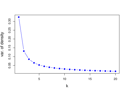
Figure 1: Dependence of the density variance on the $k$-th order of the nearest neighbour. Note the rapid decrease of variance at lower $k$ and the much shallower decrease for larger values.

The Figure helps us to estimate the optimal selection of the $k$ value. Up to $k=5$ the variance drops rapidly and starting about $k=8$ its change is much shallower. We select the values of $k=8,10,12,14$ and study densities in these four representative cases. The simulated 10000 runs enable us to calculate the mean and variance of the density at every GRB location in the sample. Using the variance and the mean of the density we calculate the standardized (zero mean and unit variance) values of the density for all points of the sample. In Figure 2 we display a scatter plot between the standardized logarithmic density and the comoving distance for the cases of $k=8,10,12$ and $14$, respectively.

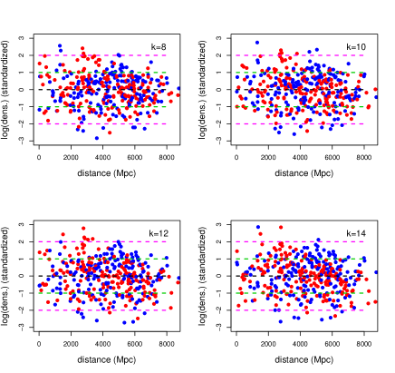
Figure 2: Dependence of the standardized logarithmic density on the comoving distance. The 0 ($mean),1\sigma,2\sigma$ lines are marked with black, green and magenta colors, respectively. The GRBs in the Southern Galactic hemisphere and those in the Northern are marked with red and blue colors. Note that a group of red points close to the $2\sigma$ line at about 2800 Mpc may correspond to a real density enhancement of GRBs in the Southern Galactic hemisphere. The GRB Great Wall discovered by Horvath et al. appears as a group of blue points between the $1\sigma$ and $2\sigma$ lines in the 4000-6000 Mpc distance range.

A quick glance at Figure 2 reveals a group of red (Southern) dots between the $1\sigma$ and $2\sigma$ lines at about 2800 Mpc. These dots may represent an associated group of GRBs. The Great GRB Wall discovered by Horvath et al. can be recognized as an enhancement of blue (Northern) dots between the $1\sigma$ and $2\sigma$ lines in the 4000-6000 Mpc distance range. These impressions, however, are somewhat subjective, their validity needs to be confirmed by some suitable statistical study for a more formal significance.

The null hypothesis in this case is the assumption that all spatial density enhancements of GRBs are produced purely by random fluctuations. Assuming the validity of the null hypothesis one has to compute the probability of the density enhancement in question. We perform a series of Kolmogorov-Smirnow (KS) tests and confirm that the standardized logarithmic densities displayed in Figure 2 follow a Gaussian distribution. Denoting the logarithmic density by $\varrho$, the probability that the $i$-th element’s value is a density enhancement is $p_{i}\propto exp(-\varrho^{2}_{i}/2)$ and the log-likelihood function has the form

$$L=-\frac{1}{2}\sum\limits^{n}_{i=1}\varrho^{2}_{i}+const.$$ (10)

The summation in Equation (10) yields a $\chi^{2}_{n}$ variable with $n$ degrees of freedom. All density fluctuations are restricted within certain distance ranges. To get a likelihood function sensitive to a given density enhancement and/or deficit we have to sum up successive points in Equation (10). Taking and summing up $k$ successive points within a distance range we get a $\chi^{2}_{k}$ variable having $k$ degrees of freedom. All density values are calculated from a fixed number of nearest neighbours in the sample. We choose for $k$ the order of the nearest value from which the density is calculated.

There is some arbitrariness to this procedure. The $k$ orders of the next neighbours have been selected somewhat by insight. Nevertheless, the calculated densities correlate strongly. This property enables us to concentrate the densities into one variable.

order	k=8	k=10	k=12	k=14
k= 8	1.000	0.914	0.540	0.706
k=10	0.914	1.000	0.515	0.661
k=12	0.540	0.515	1.000	0.743
k=14	0.706	0.661	0.743	1.000

Table 1: Correlation between logarithmic densities computed from $k^{th}$ orders of nearest neighbours.

The correlation matrix in Table 1 reveals a strong correlation between nearest neighbor estimation of densities of the orders $k=8$, $k=10$, $k=12$ and $k=14$. To get a joint variable we perform principal component analysis (PCA) on the standardized logarithmic densities used above. To get the PCs we use the princomp() procedure from R’s stats library.

By running this procedure we obtain the eigenvalues given in Table 2. The eigenvalues indicate the variance of PC’s obtained. We can infer from the variances that the first PC describes 91% of the total variance. We assume, therefore, that the information from the spatial density is concentrated into this variable. From the first PC we compute the $\chi^{2}_{k}$ variables for $df=8$, $df=10$, $df=12$ and $df=14$ degrees of freedom. The results are displayed in Figure 3.

	PC1	PC2	PC3	PC4
eigen val.	3.517	0.222	0.077	0.049
st. dev.	1.875	0.472	0.279	0.221

Table 2: Eigenvalues resulting from the PCA. The values demonstrate clearly that only the first PC (marked in bold face) is significant.

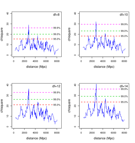
Figure 3: The calculated $\chi^{2}_{k}$ values using the first PC. Their degree of freedom is given in the right top corner of the corresponding frame.

4 Discovery and nature of the GRB ring

In all frames in Figure 3 there is a strong peak exceeding the $99.9\%$ significance level (99.95%, 99.93%, 99.96%, 99.97% at $k$=8, 10, 12, 14, respectively) at about 2800 Mpc corresponding to a group of outlying points in Figure 2. This appears to indicate the presence of some real density enhancement.

4.1 Discovery of the ring

We assume that GRBs making some contribution to the highly significant peak shown in Figure 3 lie within the full width at half maximum (FWHM) angular distance of the peak. Their angular distribution is shown in Figure 4. The most conspicuous feature in all of the frames is a ring-like structure in the lower left side of the frames. The redshift, distance and Galactic coordinates of the GRBs displaying the ring are given in Table 3. Using the data listed in the Table one can calculate the mean redshift and distance of the ring, along with the standard deviations of these variables, yielding $z=0.822$, $\sigma_{z}=0.025$ and $d_{c}=2770$ Mpc, $\sigma_{d}=65$ Mpc.

GRB ID	redshift	distance (Mpc)	l (deg)	b (deg)
040924	0.859	2866	149.05	-42.52
101225A	0.847	2836	114.45	-17.20
080710	0.845	2831	118.43	-42.96
050824	0.828	2786	123.46	-39.99
071112C	0.823	2772	150.37	-28.43
051022	0.809	2736	106.53	-41.28
100816A	0.804	2723	101.39	-32.53
120729A	0.800	2712	123.85	-12.65
060202	0.785	2672	142.92	-20.54

Table 3: Redshift, comoving distance, and galactic coordinates of the GRBs contributing to the ring-like angular structure.

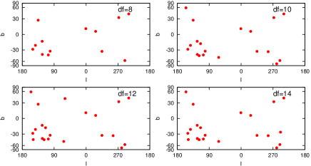
Figure 4: Angular distribution of GRBs in the $FWHM$ distance range of the highest peaks in Figure 3. The degree of freedom in the upper right corner has the same meaning as in Figure 3. Note the ring-like structure of objects in the lower left part of the frames.

By definition, the true characteristic physical size $D$ of the object can be obtained from the $D=\Theta\times d_{a}=\Theta\times d_{c}/(1+z)$ relation, where $\Theta$ is the mean angular size and $d_{a}$ is the angular distance. Substituting the corresponding values obtained above one gets $D=944$ Mpc, corresponding to 1720 Mpc in the comoving frame.

4.2 Verification of the ring structure

In subsection 4.1 we claim to find a regular structure in the shape of a ring. However, the form of this structure is thus far based only on a visual impression. In the following discussion we try to give a quantitative value supporting the sensibility of this subjective impression.

The procedure we used to obtain the very low probability of this density enhancement only by chance is not sensitive to the true shape of this clustering. Assuming this clustering to be real we may compute the probability of getting a ring-like structure only by chance by assuming some concrete space distribution for the objects. We make these calculations for the cases of a) a homogeneous sphere and b) a shell (for more details see the Appendix).

The probability of observing a ring-like structure is $p=0.2$ in the case of a shell but it is only $p=4\times 10^{-3}$ for a homogeneous sphere. It is worth noting that real space distributions of cluster members generally concentrate more strongly towards the center than do the elements of a homogeneous sphere. Therefore, this probability can be taken as an upper bound for a probability of obtaining a ring shape purely by chance.

Combining this latter probability with that of observing the clustering purely by chance we obtain a value of $p=2\times\,10^{-6}$ for observing a ring entirely by chance. Thus, despite the large angular size of the extended GRB cluster, we find evidence that the cluster represents a large extended ring in the $0.78\leq z<0.86$ redshift range.

4.3 The physical nature of the ring

If we assume that the ring represents a real structure, then we can speculate about its nature and origins. Perhaps a simple explanation is that it indicates the presence of a ring-like cosmic string. This would indicate that it is a large-scale component of the cosmic web, representing the characteristic spatial distribution of the objects in the Universe. The main difficulty with this simple explanation lies with the uniformity of the redshifts (distances) along the object, indicating that we must be seeing the ring nearly face-on. This possibility cannot be excluded, but alternative explanations are also worth of considering.

GRBs are short-lived transient phenomena. The GRBs that compose the ring, along with their redshifts, were collected over a period of about ten years. The number of observed events is determined by the time frequency of such events in a given host galaxy. However, the total number of hosts in the region containing the GRB ring and not having burst events during the observation period must be much greater relative to those which were observed.

The number of observed GRBs should be proportional to the number of progenitors in the same region, although the spatial stellar mass density is not necessarily proportional to the spatial number density of progenitors. Namely, the progenitors for the majority of GRBs are thought to be short-lived $20-40\,M_{\odot}$ stars, and as such their presence should be strongly dependent on the star formation activity in their host galaxies. Thus, our knowledge of the underlying mass distribution is sensitive to assumptions about star formation within the ring galaxies.

4.3.1 Mass of the ring

In order to estimate the mass of the ring structure we make two extreme assumptions providing lower and upper bounds for the mass. We get a lower bound for the mass by assuming that the general spatial stellar mass density is the same in the field and in the ring’s region and only the star formation and consequently the GRB formation rate is higher here. We get an upper bound for the mass by supposing a strict proportionality between the stellar mass density and the number density of the progenitors. For both estimates we need to know the local stellar density.

Several recent studies have attempted to determine the stellar (barionic) mass density and its relation to the total Universal mass density. Bahcall & Kulier (2014) determined the stellar mass fraction and found it to be nearly constant on all scales above $~{}300\,h^{-1}\,kpc$, with $M^{*}/M_{tot}\cong 0.01\pm 0.004$. Le Fèvre et al. (2013, 2014) issued the VIMOS VLT Deep Survey (VVDS) final and public data release offering an excellent opportunity to revisit galaxy evolution. The VIMOS VLT Deep Survey is a comprehensive survey of the distant universe, covering all epochs since $z\sim 6$. From this, Davidzon et al. (2013) measured the evolution of the galaxy stellar mass function from $z=1.3$ to $z=0.5$ using the first 53 608 redshifts.

Marulli et al. (2013) investigated the dependence of galaxy clustering on luminosity and stellar mass in the redshift range $0.5<z<1.1$ using the ongoing VIMOS Public Extragalactic Survey (VIPERS). Based on their sample of 10095 galaxies, Driver et al. (2007) estimated the stellar mass densities at redshift zero amounting to $8.6\,h^{-1}\pm 0.6\times 10^{8}M_{\odot}/Mpc^{3}$. We use this local value as our measure of the mass density in the comoving frame and use it for our subsequent calculations.

We assign a volume to the ring by computing the convex hull (CH) of the points representing the GRBs in the rest frame. Using the Qhull program we obtain a value of $1.9\times 10^{8}$ Mpc³ for the volume of the CH. Supposing that the stellar mass density is the same in the ring’s region (i.e. within the CH) as in the field and only the number of progenitors is enhanced we compute a mass of $2.3\times 10^{17}\,M_{\odot}$ inside the CH.

Alternatively, if we assume that the fraction of progenitors is the same along the ring as it is in the field, then the total stellar mass in the volume of a shell with 2770 Mpc radius and 200 Mpc thickness (the observed distance range of the GRBs in the ring) is $2.2\times 10^{19}\,M_{\odot}$. Since the number of GRBs making up the ring is about the half the total observed in the shell, we get a mass of $1.1\times 10^{19}\,M_{\odot}$ within the ring’s CH.

Supposing a strict proportionality between the spatial densities of the number of GRB progenitors and stellar masses we estimate a factor of 50 times more mass than that which is obtained above using the field value within the CH. In the case of a homogeneous mass distribution within the CH this implies an overdensity by a factor of 50 compared to the field.

In reality, however, the overdensity within the CH appears to be concentrated in the outer half of its volume in order to produce a ring-like distribution, suggesting an overdensity enhanced by a factor of more than 100. This high value appears to be unrealistic. To resolve this contradiction, the proportion of progenitors in the stellar mass has to be increased by at least an order of magnitude and the stellar mass density has to be decreased by the same factor in the outer half volume of the CH. This results in a value of $1\times 10^{18}\,M_{\odot}$, which still represents an overdensity of a factor of 10 suggesting the ring mass is in the range $10^{17}-10^{18}\,M_{\odot}$, depending on the fraction of progenitors in the stellar mass distribution.

4.3.2 The case for a spheroidal structure

To overcome the difficulty caused by the low probability of seeing a ring nearly face on one may assume the GRBs populate the surface of a spheroid which we see in projection. To demonstrate that the projection of GRBs uniformly populating the surface of the spheroid really can produce a ring in projection, we make MC simulations displayed in Figure 5. The simulations show that a ring structure can be obtained easily by projecting a spheroidal shell onto a plane. The probability of observing a ring in this way is much larger than that of observing a ring face on.

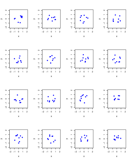
Figure 5: Monte Carlo simulation of projecting points into a plain, distributed uniformly on a sphere. It is worth noting that some of the simulations strongly resemble the observed ring.

Unfortunately, this approach also faces some problems. Assuming the observed ring is a projection onto a plane, one can calculate the standard deviation of distances of the objects to the observer. A simple calculation shows this standard deviation is about 58% of the radius in case of a sphere. Previously we obtained 1720 Mpc for the diameter of the ring resulting in a 860 Mpc radius with a 499 Mpc standard deviation for the comoving distances. With the projection correction, however, we obtain only 65 Mpc for this value. This result is obviously in tension with the value of the standard deviation assuming a spherical distribution for the GRBs displaying the ring.

The relatively low standard deviation of the distances, however, is not necessarily caused by some physical property of the structure but could be caused by the $FWHM$ of the statistical signal. Increasing the distance range around the peak of the statistical signal relative to the value of the standard deviation increases the foreground/background as well, and indicates that the structure may be buried in the noise. Nevertheless, for the case of a projected sphere increasing the distance range in this way implies that the total number of GRBs displaying this structure also has to be increased by a factor of 6. This would cause the $FWHM$ of the statistical signal to be much wider, in contrast to what is observed.

One may resolve this tension somewhat arbitrarily in the following way. The 499 Mpc value for the standard deviation of the comoving distances was obtained by assuming a shell-like GRB distribution. Let us take an interval around the mean distance of 2770 Mpc within the standard deviation of 499 Mpc. The endpoints correspond to some lookback time difference between GRBs detected at the same moment by the observer. The lookback time can be calculated from the following equation:

$$t_{L}(z)=t_{H}\int^{z}_{0}\frac{dz^{\prime}}{(1+z^{\prime})\sqrt{\Omega_{M}(1+z^{\prime 3})+\Omega_{\Lambda}}}$$ (11)

where $t_{H}=1/H_{0}$ is the Hubble time. Calculating the time difference one obtains $\Delta t_{L}=1.9\times 10^{9}$ years. Computing the time difference taking the observed 65 Mpc standard deviation instead of 499 Mpc, one gets only $\Delta t_{L}=2.5\times 10^{8}$ years. If the GRBs displaying the observed ring really populate a sphere, then the presence of the low 65 Mpc standard deviation reveals a $2.5\times 10^{8}$ year period in the life of the host galaxy when it is very active in producing GRBs. Furthermore, one has to assume that this happens for all hosts simultaneously. This coordinated activity may happen by some external effect which is responsible for the formation of the sphere.

One can make a similar estimate of the sphere’s mass by assuming that the ring represents a real structure and is not simply a projection. The difference in this case is that the ring mass represents only a fraction of the sphere’s mass. There are 7 objects in the ring within the 65 Mpc standard deviation. There is a factor of 7 for getting the number of GRBs within $1\sigma$ on the sphere. This number represents 68% of the total number of GRBs on the sphere, i.e. one should multiply the mass obtained for the ring by roughly a factor of ten, yielding $10^{18}-10^{19}\,M\odot$ for the sphere.

4.3.3 Formation of the ring

No matter whether we interpret the spatial structure of the ring as a torus or as a projection of a spheroidal shell, the formation of a structure with this large size and mass provides a real challenge to theoretical interpretations. In addition to the size and the mass of the structure, one has to explain why the GRB activity is much higher along the ring than it typically is in the field.

There is general agreement among researchers that following the early phase of the Big Bang the initial perturbations evolved into a cosmic web consisting of voids surrounded by string-like structures. A filamentary structure surrounding sphere-like voids is a typical result of gravitational collapse (Centrella & Melott, 1983; Icke, 1984).

The hierarchy of structures in the density field inside voids is reflected by a similar hierarchy of structures in the velocity field (Aragon-Calvo & Szalay, 2013). The void phenomenon is due to the action of two processes: the synchronisation of density perturbations of medium and large scales, and the suppression of galaxy formation in low-density regions (Einasto et al., 2011).

It is generally assumed that the maximal size of these structures is $100-150$ Mpc (Frisch et al., 1995; Einasto et al., 1997; Suhhonenko et al., 2011; Aragon-Calvo & Szalay, 2013). Quite recently Tully et al. (2014) discovered the local supercluster (the ”Laniakea”) having a diameter of 320 Mpc. This scale is several times smaller than the estimated 1720 Mpc diameter of the GRB ring, although perturbations on larger scales cannot be excluded. However, Doroshkevich & Klypin (1988) have presented arguments that perturbations on the $200-300$ Mpc scale should be excluded. This value is in a clear contradiction to the existence of the GRB ring and other large observed structures. Resolution of this contradiction is still an open issue.

The existence of the ring, either as a torus or the projection of a spheroidal shell, requires a higher spatial frequency of the progenitors along the ring than in the field. A possible interpretation of the higher fraction of progenitors along the ring is that hosts are still in the formation process at $6.7\times 10^{9}$ years after the Big Bang. This supports the view that large scale structure can form and evolve slowly from the initial perturbations (Zeldovich, Einasto & Shandarin, 1982; Einasto et al., 2006).

Dark matter must be given a dominant role in large-scale structure theories in order to account quantitatively for the formation and evolution of the cosmic web. That is because the observed distributions of galaxies are inconsistent with gravitational clustering theories and with the formation of super clusters in a wholly gaseous medium (Einasto, Joeveer & Saar, 1980). Recent extensive numerical studies that include dark matter indicate that its presence accounts for the basic properties of the cosmic web (Springel et al., 2005; Angulo et al., 2012), and these studies have reproduced the cosmic star formation history and the stellar mass function with some success (Vogelsberger et al., 2013). The very large high-resolution cosmological N-body simulation, the Millennium-XXL or MXXL (Angulo et al., 2012), which uses 303 billion particles, modeled the formation of dark matter structures throughout a 4.1 Gpc box in a $\Lambda CDM$ cold dark matter cosmology. Kim et al. (2011) presented two large cosmological N-body simulations, called Horizon Run 2 (HR2) and Horizon Run 3 (HR3), made using $6000^{3}=216$ billions and $7210^{3}=374$ billion particles, spanning a volume of $(7.200\,h^{-1}Gpc)^{3}$ and $(10.815\,h^{-1}Gpc)^{3}$, respectively. Although these sizes of the simulated volumes were large enough to produce very large structures, accounting for local enhancements corresponding to the size of the GRB ring structure is still an open problem. We address this issue in the next subsection.

4.3.4 Spatial distribution of GRBs and large scale structure of the Universe

In subsection 4.3.3 we noted that very large scale cosmological simulations may account for huge disturbances in the dark matter distribution, in particular for LQGs and the object discovered by Horváth, Hakkila & Bagoly (2013). Nevertheless, in subsections 4.3.1 and 4.3.2 we pointed out that the existence of the GRB ring probably can not be accounted for a simple enhancement of the underlying barionic and dark matter density. Presumably, to explain the existence of the ring one needs a coordinated enhanced GRB activity in the responsible host galaxies.

According to a widely accepted view the majority of the observed GRBs are resulted in collapsing high mass ($20-40\,M_{\odot}$) stars. GRBs are very rare transient phenomena, consequently, they observed spatial distribution is a serious under sampling of the space distribution of galaxies in general. Furthermore, the high mass stars have short lifetimes, consequently GRBs prefer those galaxy hosts having considerable star forming activity.

Due to their immense intrinsic brightnesses, GRBs can be detected at large cosmological distances. GRB 090423 has $z=8.2$, the largest spectroscopically measured redshift (Tanvir et al., 2009). Even though GRBs seriously under-sample the matter distribution, they are the only observed objects doing so for the Universe as a whole up to the distance corresponding to the largest measured redshift.

Since there is no complete observational information on the spatial distribution of dark and barionic matter on the same scale as that of GRBs, one has to use the large scale simulations of the distribution of the cosmic matter for making such comparisons. We used for this purpose the publicly available Millennium-XXL simulation.

As we mentioned at the end of subsection 4.3.3, the 4.1 Gpc size of the simulated volume is large enough to account for structures with characteristic size of the ring. Since GRBs prefer host galaxies with high star formation activity, we calibrate the dark matter density in XXL to the spatial number density of galaxies having large star forming rate ($SFR$) assuming that

$$\nu_{s}(x,y,z))=c(\varrho_{d})\varrho_{d}(x,y,z)$$ (12)

where $\nu_{s}$ represents the spatial number density of star forming galaxies and $\varrho_{d}$ the density of the dark matter. We assume that the $c(\varrho_{d})$ conversion factor depends only on $\varrho_{d}$ but not on the spatial coordinates and that it is identical in the XXL and the Millennium simulation.

We determine the $c(\varrho_{d})$ conversion factor using the data available in the Millennium simulation. The GRB ring is located in the $0.78<z<0.86$ redshift range, so we select the $z=0.82$ slice of the simulation. The star forming galaxies have $SFR>30\,M_{\odot}\,yr^{-1}$ at this redshift (Perley et al., 2015).

As one can infer from Figure 6, the selected star forming galaxies prefer a certain dark matter density range: for densities less than and greater this range such galaxies are uncommon in the sample. This range differs from that of galaxies in general. This may indicate that the spatial distribution displayed by the galaxies in general is not necessary identical with that shown by the GRBs.

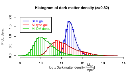
Figure 6: Probability distribution of the dark matter density in the Millennium simulation. Distribution of dark matter density in the simulation (green), for galaxies in general (red), and for star forming galaxies (blue). The star forming galaxies prefer a certain range of underlying dark matter density that differs from that of galaxies in general.

After determining the $c(\varrho_{d}$) conversion factor, we obtain from Equation (6) the $\nu_{s}$ spatial number density of the star forming galaxies in the XXL simulation. Based on this spatial distribution we generate random samples of sizes comparable to that of the observed GRB frequency. For generating the simulated sample we use the Markov Chain Monte Carlo (MCMC) method implemented in the metrop() procedure available in R’s mcmc library.

An important issue for using this algorithm is to check whether or not the simulated Markov chain has reached its stationary stage. We check it by computing the auto regression function of the simulated sample by the acf() function in R. We also check the MCMC output by conventional MC.

The known number of GRBs now exceeds a couple of thousand and is steadily increasing with ongoing observations. Unfortunately, only a fraction of these have measured redshifts. Motivated by the number of known GRBs and by their relationship to star forming galaxies, we make MCMC simulations of the $\nu_{s}(x,y,z)$ spatial number density of these galaxies from Equation (6), getting sample sizes of 1000, 5000, 10000 and 20000.

We make 100 simulations for these sample sizes and compare them with completely spatially random (CSR) samples of the same sizes in the XXL volume. In subsection 3.3 we computed the nearest neighbors of the $k=8,10,12$ and $14$ order. Following the same procedure here, we obtain the nearest neighbor distances of the $k=12^{th}$ order for the XXL and the CSR samples and using the ks.test() procedure in R’s stats library, and compute the maximal difference between the cumulative distributions. We repeat this procedure between the CSR nearest neighbor distributions. The distributions of KS differences between XXL-CSR and CSR-CSR samples are displayed in Figure 7.

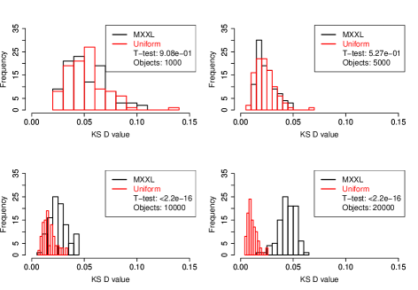
Figure 7: Comparison of the KS differences between the XXL and CSR (black) and the CSR (red) cumulative distributions of the $k=12^{th}$ nearest neighbors distances. Note the significant differences between the XXL and CSR case at sample sizes of N=10000 and 20000 (bottom left and right) unlike to N=1000 and 5000 (top left and right) where there are no significant differences.

As one may infer from this figure, the distribution of KS differences between XXL-CSR samples do not differ significantly from those of CSR-CSR in the case of the sample sizes of $N=1000$ and 5000. On the contrary, in the case of $N=10000$ and 20000 the difference between the XXL-CSR and CSR-CSR cases is very significant.

Based on this result one may conclude that the simulated XXL samples with sizes of $N=1000$ and 5000 do not differ from the CSR case. On the other hand, the samples with sizes of $N=10000$ and 20000 differ significantly from the CSR case. Each sample corresponds to some mean distance to the nearest object of the $k=12^{th}$ order. The computed mean distances are tabulated in Table 4.

Obviously, groups having a characteristic size of 280 Mpc can be detected with a sufficiently large sample size. This value corresponds to the largest structure (251 Mpc) found by Park et al. (2012) using the HR2 simulation. The number of GRBs detected, however, is insufficient for revealing this scale. Consequently, if the XXL simulation correctly represents the large scale structure of the Universe the GRBs reveal it as CSR on the scale corresponding to the sample size.

At this point, however, it may be appropriate to repeat the remark made at the beginning of this subsection: the existence of the GRB ring can not be explained by a simple density enhancement of the underlying barionic and/or dark matter. It probably needs some coordinated star forming activity among the responsible GRB hosts. In this case the spatial distribution of GRBs does not necessarily trace the underlying matter distribution in general. However, we can not exclude the possibility that the XXL simulation does not correctly account for all possible large scale structures and GRBs are mapping a structure that was not simulated.

Sample size	Mean dist. [Mpc]	Prob. of CSR
1000	627	0.39
5000	351	0.71
10000	277	${\bf<2.2e-16}$
20000	217	${\bf<2.2e-16}$

Table 4: Mean distances to the $k=12^{th}$ order nearest neighbor of star forming galaxies at different sample sizes in the XXL simulation and the probability for being CSR. The significant deviation from the CSR case is marked in bold face. Note that this size is consistent with the CP and more than six times smaller than the GRB ring in this paper.

Some concern may arise, however, concerning the interpretation of the ring as a true physical structure, and of the causal relationship between the GRBs displaying it. Suhhonenko et al. (2011) has pointed out that cosmic structures greater than 140 Mpc in co-moving coordinates did not communicate with one another during the late stage of universal expansion preceding Recombination. The skeleton of the web was created during the inflationary period (Kofman & Shandarin, 1988) and evolved slowly following this epoch.

The volume of the shell between $0.78<z<0.86$ is $20.2\,Gpc^{3}$ in the co-moving frame. The corresponding volume is $2.1\,Gpc^{3}$ for $z=0.2$ in the case of the SDSS main sample and $14.4\,Gpc^{3}$ for $z=0.4$ for luminous red galaxies (LRGs), respectively. The volume of the shell is about ten thousand times larger than the volume of a typical supercluster found by Liivamägi, Tempel & Saar (2012) in the SDSS data.

Since the cosmic web evolves slowly, the structure of the GRB ring should exhibit the same general characteristics as those displayed by superclusters defining the web. Comparing the estimated number of superclusters with the number of detected GRBs, it appears that every thousand superclusters has produced on average one measured GRB. GRBs are therefore very rare events superimposed on the web, and the small probability of GRB detection casts serious doubt on the nature of the GRB ring as a real physical structure.

Taking these distributional characteristics into account suggests that the Ring is probably not a real physical structure. Further studies will be needed to reveal whether or not the Ring structure could result from a low-frequency spatial harmonic of the large-scale matter density distribution and/or of universal star forming activity.

5 Summary and conclusion

Motivated by the recent discovery of Horváth, Hakkila & Bagoly (2013) revealing a large Universal structure displayed by GRBs, we study the spatial distribution of these objects in the comoving frame. The advantage of this approach is that GRBs (which are short transients) have footprints in this frame that do not change with time.

We assume in this approach that, for the spatially homogenous and isotropic case, the joint observed distribution of the GRBs can be factored into two parts: one part depends on the angular coordinates while the other part is radial and depends on the redshift.

This assumption can be tested in two different ways. The first method is essentially that used by Horvath et al. which compares the conditional probability of the GRB angular distribution at different $z$ values. The second method tests whether resampling the GRBs randomly makes any statistical changes in the distribution in the 3D comoving frame.

We estimate the spatial density of GRBs by searching the angular separations of the $k$-th order nearest neighbours. For these computations we use the knn.dist(x,k) procedure in the FNN library of the R statistical package. To compromise between the large variance of estimated densities at small $k$ values and the smearing out of real small scale structures at large $k$ values, we use the spatial densities obtained by taking $k=8,10,12$ and $14$.

Resampling the redshift distribution 10000 times and calculating the spatial densities from the samples obtained in this way we obtain mean densities and their variances assuming the null hypothesis, i.e. that the factorization of the spatial distribution of GRBs is valid. Subtracting the mean value from the observed one and dividing by the standard deviation we calculate the standardized values of the densities obtained from the nearest neighbour procedure.

KS tests revealed that the logarithmic densities obtained in this way follow a Gaussian distribution allowing us to get a logarithmic likelihood function as a sum of the squared logarithmic densities. Since the sum of squared Gaussian variables follows a $\chi^{2}_{k}$ distribution with $k$ degrees of freedom, by selecting objects in a certain distance separation range and calculating the value of this variable we can test for the significance of density fluctuations.

Since the calculated logarithmic densities in the $k=8,10,12,14$ cases are strongly correlated pairwise, performing a principal component analysis (PCA) allows us to join the logarithmic densities in the first (the only significant) PC variable representing 91% of the total variance. Computing $\chi^{2}_{k}$ values from this PC for $k=8,10,12,14$ degrees of freedom and plotting them as a function of the distance, we find a very pronounced peak at about 2800 $Mpc$ corresponding to a significance of 99.95%, 99.93%, 99.96% and 99.97%, depending on the degrees of freedom.

We plot the angular positions of the GRBs within the $FWHM$ range around the distance of the $\chi^{2}_{k}$ peak. Examining these plots we conclude the following:

• There is a ring consisting of 9 GRBs having a mean angular diameter of $36^{o}$ corresponding to 1720 Mpc in the comoving frame.

• The ring is located in the $0.78<z<0.86$ redshift range having a standard deviation of $\sigma_{z}=0.025$, corresponding to a comoving distance range of $2672<d_{c}<2866$ Mpc having a standard deviation of $\sigma_{d}=65\,Mpc$.

• If one interprets the ring as a real spatial structure, then the observer has to see it nearly face on because of the small standard deviation of GRB distances around the object’s center.

• The ring can be a projection of a spheroidal structure. Adopting this approach one has to assume that each host galaxy has a period of $2.5\times 10^{8}$ years during which the GRB rate is enhanced.

• The mass of the object responsible for the observed ring is estimated to be in the range of $10^{17}-10^{18}\,M\odot$ if the true structure is a torus or $10^{18}-10^{19}\,M\odot$ in case of a spheroid.

• GRBs are very rare events superimposed on the cosmic web identified by superclusters. Because of this, the ring is probably not a real physical structure. Further studies are needed to reveal whether or not the Ring could have been produced by a low-frequency spatial harmonic of the large-scale matter density distribution and/or of universal star forming activity.

Appendix A Observing a ring structure by chance

In this manuscript we have found strong evidence for a ring-like structure displayed by 9 GRBs. The probability of obtaining this clustering only by chance is about $p=5\times 10^{-4}$, but this value is not sensitive to the actual pattern of the points within the group. Although we claim to have found evidence for a regular structure, the apparent shape of a ring is based only on a visual impression. It is useful to develop a quantitative measure supporting the efficacy of this subjective impression.

In this appendix we compare the projection of two simple spherical models; a) a homogeneous sphere and b) a spherical shell. It is not difficult to derive the probability density functions for these projections into a plain. If we denote the projected distance from the mean position of the group to one of the members by $\varrho$, then we can normalize each position relative to the maximum projection $\varrho_{max}$ so that the projections vary in the range of {0,1}. In case of a homogeneous sphere the projected probability density is given by

$$f(\varrho)=3\varrho\sqrt{1-\varrho^{2}}$$ (13)

and in the case of a shell we get

$$g(\varrho)=\frac{\varrho}{\sqrt{1-\varrho^{2}}}$$ (14)

The shapes of these functions are displayed in Figure 8.

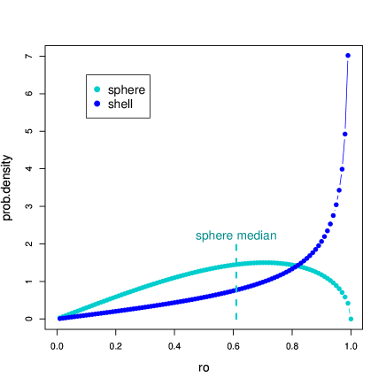
Figure 8: Comparison of the projected probability densities of a homogeneous sphere and a shell. The median of the sphere is indicated.

The Figure demonstrates that the projections for a shell result in a significant enhancement of the points close to the maximal distance from the center; this is not the case for a projected homogenous sphere. We can compute the probability of measuring all 9 points outside of the median distance. By definition the median splits the distribution into two parts of equal probability. The value of the median distance for a projected homogeneous sphere is $\varrho_{median}=0.61$.

We can calculate the probability of measuring all 9 points in the ${0.61<\varrho<1}$ regime. To calculate the probability of this case we invoke the binom.test() procedure available in the R statistical package. The probability of finding an object outside the median distance is $p=0.5$ by definition. The probability for finding all 9 points outside the median is given by the binomial distribution.

Similarly we can calculate the probability of having all 9 objects in a region outside the $\varrho_{median}=0.61$ median, assuming that the true spatial distribution of the points is a shell. Integrating the $g(\varrho)$ probability density in the {0.61, 1} interval we get

$$\int\limits^{1}_{0.61}g(\varrho)=\int\limits^{1}_{0.61}\frac{\varrho}{\sqrt{1-\varrho^{2}}}=0.7924$$ (15)

Inserting this probability into the binomial test expression we get $p=0.2192$.

Summarizing the results of the tests performed above, we infer that the probability of observing a ring-like structure from a projected 3D homogeneous density enhancement only by chance is $p=3.9\times 10^{-3}$ while assuming a projected 3D shell it is much higher, $p=0.22$. This gives us a good reason to believe that the ring is a result of a projected 3D shell-like regular pattern.

References

- Angulo et al. (2012) Angulo R. E., Springel V., White S. D. M., Jenkins A., Baugh C. M., Frenk C. S., 2012, MNRAS, 426, 2046
- Aragon-Calvo & Szalay (2013) Aragon-Calvo M. A., Szalay A. S., 2013, MNRAS, 428, 3409
- Bagla, Yadav & Seshadri (2008) Bagla J. S., Yadav J., Seshadri T. R., 2008, MNRAS, 390, 829
- Bahcall & Kulier (2014) Bahcall N. A., Kulier A., 2014, MNRAS, 439, 2505
- Balazs, Meszaros & Horvath (1998) Balazs L. G., Meszaros A., Horvath I., 1998, A&A, 339, 1
- Balázs et al. (1999) Balázs L. G., Mészáros A., Horváth I., Vavrek R., 1999, A&AS, 138, 417
- Briggs (1993) Briggs M. S., 1993, ApJ, 407, 126
- Castro Cerón et al. (2010) Castro Cerón J. M., Michałowski M. J., Hjorth J., Malesani D., Gorosabel J., Watson D., Fynbo J. P. U., Morales Calderón M., 2010, ApJ, 721, 1919
- Centrella & Melott (1983) Centrella J., Melott A. L., 1983, Nature, 305, 196
- Clowes et al. (2012) Clowes R. G., Campusano L. E., Graham M. J., Söchting I. K., 2012, MNRAS, 419, 556
- Clowes et al. (2013) Clowes R. G., Harris K. A., Raghunathan S., Campusano L. E., Söchting I. K., Graham M. J., 2013, MNRAS, 429, 2910
- Clowes, Iovino & Shaver (1987) Clowes R. G., Iovino A., Shaver P., 1987, MNRAS, 227, 921
- Davidzon et al. (2013) Davidzon I. et al., 2013, A&A, 558, A23
- Doroshkevich et al. (2004) Doroshkevich A., Tucker D. L., Allam S., Way M. J., 2004, A&A, 418, 7
- Doroshkevich & Klypin (1988) Doroshkevich A. G., Klypin A. A., 1988, MNRAS, 235, 865
- Driver et al. (2007) Driver S. P., Popescu C. C., Tuffs R. J., Liske J., Graham A. W., Allen P. D., de Propris R., 2007, MNRAS, 379, 1022
- Einasto et al. (1997) Einasto J. et al., 1997, Nature, 385, 139
- Einasto et al. (2006) Einasto J. et al., 2006, A&A, 459, L1
- Einasto & Gramann (1993) Einasto J., Gramann M., 1993, ApJ, 407, 443
- Einasto, Joeveer & Saar (1980) Einasto J., Joeveer M., Saar E., 1980, Nature, 283, 47
- Einasto et al. (2011) Einasto J. et al., 2011, A&A, 534, A128
- Einasto et al. (2014) Einasto M. et al., 2014, A&A, 568, A46
- Ellis (1975) Ellis G. F. R., 1975, QJRAS, 16, 245
- Frisch et al. (1995) Frisch P., Einasto J., Einasto M., Freudling W., Fricke K. J., Gramann M., Saar V., Toomet O., 1995, A&A, 296, 611
- Gott et al. (2005) Gott, III J. R., Jurić M., Schlegel D., Hoyle F., Vogeley M., Tegmark M., Bahcall N., Brinkmann J., 2005, ApJ, 624, 463
- Graham, Clowes & Campusano (1995) Graham M. J., Clowes R. G., Campusano L. E., 1995, MNRAS, 275, 790
- Haberzettl et al. (2009) Haberzettl L. et al., 2009, ApJ, 702, 506
- Haines, Campusano & Clowes (2004) Haines C. P., Campusano L. E., Clowes R. G., 2004, A&A, 421, 157
- Heinämäki et al. (2005) Heinämäki P., Suhhonenko I., Saar E., Einasto M., Einasto J., Virtanen H., 2005, ArXiv e-prints 0507197