A Characterization of the Complexity of Resilience and Responsibility for Self-join-free Conjunctive Queries

Abstract

Several research thrusts in the area of data management have focused on understanding how changes in the data affect the output of a view or standing query. Example applications are explaining query results, propagating updates through views, and anonymizing datasets. These applications usually rely on understanding how interventions in a database impact the output of a query. An important aspect of this analysis is the problem of deleting a minimum number of tuples from the input tables to make a given Boolean query false. We refer to this problem as “the resilience of a query” and show its connections to the well-studied problems of deletion propagation and causal responsibility. In this paper, we study the complexity of resilience for self-join-free conjunctive queries, and also make several contributions to previous known results for the problems of deletion propagation with source side-effects and causal responsibility: (1) We define the notion of resilience and provide a complete dichotomy for the class of self-join-free conjunctive queries with arbitrary functional dependencies; this dichotomy also extends and generalizes previous tractability results on deletion propagation with source side-effects. (2) We formalize the connection between resilience and causal responsibility, and show that resilience has a larger class of tractable queries than responsibility. (3) We identify a mistake in a previous dichotomy for the problem of causal responsibility and offer a revised characterization based on new, simpler, and more intuitive notions. (4) Finally, we extend the dichotomy for causal responsibility in two ways: (a) we treat cases where the input tables contain functional dependencies, and (b) we compute responsibility for a set of tuples specified via wildcards.

1 Introduction

As data continues to grow in volume, the results of relational queries become harder to understand, interpret, and debug through manual inspection. Data management research has recognized this fundamental need to derive explanations for query results and explanations for surprising observations. Existing work has defined explanations as predicates in a query [Wu and Madden (2013), Roy and Suciu (2014), Chapman and Jagadish (2009)], or as modifications to the input data [Meliou et al. (2010), Huang et al. (2008), Herschel et al. (2009)]. In the latter category, the metric of causal responsibility, first introduced by ChocklerH04, quantifies the contribution of an input tuple to a particular output. One can then derive explanations by ranking input tuples using their responsibilities: tuples with high degree of responsibility are better explanations for a particular query result than tuples with low responsibility [Meliou et al. (2010)].

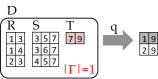
(a) Source-side effects: $\min|\Gamma|$

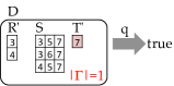
(b) Resilience: $\min|\Gamma|$

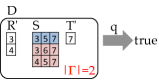
(c) Responsibility: $\min|\Gamma|$

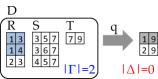
(d) View-side effects: $\min|\Delta|$

SJ: Queries with selections and joins	$\mathsf{PTIME}$	[Buneman et al. (2002)]
PJ: Queries with projections and joins	NP-complete
“Key-preserving” SPJ queries	$\mathsf{PTIME}$	[Cong et al. (2012)]
All other SPJ queries	NP-complete
“Triad-free” SPJ queries	$\mathsf{PTIME}$
All other SPJ queries	NP-complete	this paper
“FD-induced triad-free” SPJ queries	$\mathsf{PTIME}$
All other SPJ queries	NP-complete	this paper

(e) Source-side effect problem: prior and our dichotomy results

SJ: Queries with selections and joins	$\mathsf{PTIME}$	[Buneman et al. (2002)]
PJ: Queries with projections and joins	NP-complete
“Key-preserving” SPJ queries	$\mathsf{PTIME}$	[Cong et al. (2012)]
All other SPJ queries	NP-complete
“Head-dominated” SPJ queries	$\mathsf{PTIME}$	[Kimelfeld et al. (2012)]
All other SPJ queries	NP-complete
“Functional head-dominated” SPJ queries	$\mathsf{PTIME}$	[Kimelfeld (2012)]
All other SPJ queries	NP-complete

(f) View-side effect problem: prior dichotomy results

Figure 1: This paper contains dichotomy results for (a) deletion propagation with source-side effects, (b) resilience, and (c) responsibility for causality. Besides others, they imply a complete dichotomy for the source side-effect problem for the class of self-join-free conjunctive queries in the presence of functional dependencies (e). Thus, this part of our work is similar in scope to [Kimelfeld et al. (2012)] and [Kimelfeld (2012)] for the problem of view-side effects (f). We derive these results by analyzing a simpler concept: the resilience of Boolean queries. In addition (not shown in the figure), we provide a correction to a prior dichotomy result for causal responsibility and then extend it in two ways: responsibility for tables with functional dependencies and responsibility for tuples with wildcards, e.g., $S(*,5,7)$.

A seemingly unrelated notion, the concept of deletion propagation with source side-effects [Buneman et al. (2002)], seeks a minimum set of tuples in the input tables that should be deleted from the database in order to delete a particular tuple from a query. Query results that have a larger set of tuples that need to be deleted are more reliable or more “robust” to changes in the input database than others. This measure of relative importance can provide another type of explanation and allows us to rank the output tuples by their relative robustness.

In this paper, we take a step back and re-examine how particular interventions (tuple deletions in the input of a query) impact its output. Specifically, we study how “resilient” a Boolean query is with respect to such interventions. Resilience identifies the smallest number of tuples to delete from the input to make the query false. We will show that characterizing the complexity of this problem also allows us to study the complexities of both deletion propagation with source side-effects and causal responsibility with minor modifications.

Deletion propagation and existing results. Databases allow users to interact with data through views, which are often conjunctive queries. Views can be used to simplify complex queries, enforce access control policies, and preserve data independence for external applications. Of particular interest is how deletions in the input data affect the view (which is a trivial problem), but also how deletions in the view could be achieved by appropriately chosen deletions in the input data (which is far less trivial). Concretely, the problem of deletion propagation [Buneman et al. (2002), Dayal and Bernstein (1982)] seeks a set $\Gamma$ of tuples in the input tables that should be deleted from the database in order to delete a particular tuple from the view. Intuitively, this deletion should be achieved with minimal side-effects, where side-effects are defined with either of two objectives: (a) deletion propagation with source side-effects ($\mathtt{DP_{source}}$) seeks a minimum set of input tuples $\Gamma$ in order to delete a given output tuple; whereas (b) deletion propagation with view side-effects ($\mathtt{DP_{view}}$) seeks a set of input tuples $\Gamma$ that results in a minimum number of output tuple deletions in the view, other than the tuple of interest [Buneman et al. (2002)].

Example 1.1 (Source & View side effects).

Consider the query

$$q(x,u){\,:\!\!-\,}R(x,y),S(y,z,w),T(w,u)$$

defining a view over the database $R,S,T$ shown below. To delete tuple $v_{1}$ from the resulting view with minimum source side-effects, one only needs to remove tuple $t_{1}$ from the database. Therefore, the optimal solution to $\mathtt{DP_{source}}$ is $\Gamma=\{t_{1}\}$ with $|\Gamma|=1$ (see 1a).

However, the deletion of $t_{1}$ also removes $v_{2}$, which is a view side-effect: $\Delta=\{v_{2}\}$ with $|\Delta|=1$. The optimal solution to $\mathtt{DP_{view}}$, which minimizes the side-effects on the view (set $\Delta$) is the set of input tuples $\Gamma=\{r_{1},r_{2}\}$: deleting these two tuples removes only $v_{1}$ from the view but not $v_{2}$, and thus has no view-side effects, i.e., $\Delta=\emptyset$ with $|\Delta|=0$ (see 1d).

	$R$				$S$					$T$				$q$
	$X$	$Y$			$Y$	$Z$	$W$			$W$	$U$			$X$	$U$
$r_{1}$	1	3		$s_{1}$	3	5	7		$t_{1}$	7	9		$v_{1}$	1	9
$r_{2}$	1	4		$s_{2}$	3	6	7						$v_{2}$	2	9
$r_{3}$	2	3		$s_{3}$	4	5	7

Known complexity results. Buneman:2002 showed that both variants are in general NP-complete for conjunctive queries containing projections and joins (PJ), whereas they are in $\mathsf{PTIME}$ for queries containing only selections and joins (SJ). Later, Cong12 identified a class of PJ queries, called “key-preserving,” for which both problem variants can be solved in $\mathsf{PTIME}$. According to these two results, the query from Example 1.1 falls into the general class of NP-complete queries.

In addition, KimelfeldVW12 provided a more refined dichotomy result for the problem of minimal view side-effects for self-join-free conjunctive queries (CQs). This dichotomy leads to more polynomial time cases, as it characterizes the complexity based on a property of the query structure (using the property of “head domination”), rather than high-level database operators (e.g., projections and joins). For example, the query of Example 1.1 is not head-dominated, which means that $\mathtt{DP_{view}}$ is indeed NP-complete for that query. Later work has also extended the dichotomy result to self-join-free CQs with functional dependencies (FDs) [Kimelfeld (2012)].

Causal responsibility and existing results. The problem of causal responsibility [Meliou et al. (2010)] seeks, for a given query and a specified input tuple, a minimum set of other input tuples $\Gamma$ that, if deleted would make the tuple of interest “counterfactual,” i.e., the query would be true with that tuple present, or false if the tuple was also deleted. Both problems of resilience and of causal responsibility rely on the notion of minimal interventions in the input database and are thus closely related. However, we will show that resilience is easier (has lower complexity) than responsibility, and provide extensive discussion of the connections among all these related problems.

Example 1.2 (Resilience & Causal responsibility).

Consider again the query from Example 1.1 and the output tuple $v_{1}=(1,9)$. Applying the substitution $[(x,u)/(1,9)]$, i.e., substituting the variables $x$ and $u$ with 1 and 9, respectively, we get a query $q(1,9){\,:\!\!-\,}R(1,y),$ $S(y,z,w),T(w,9)$. The solution to $\mathtt{DP_{source}}$ for $q$ and tuple $v_{1}$ is then equivalent to the solution of the resilience problem over the Boolean query $q^{\prime}{\,:\!\!-\,}R^{\prime}(y),S(y,z,w),T^{\prime}(w)$ over the database $R^{\prime},S,T^{\prime}$ with $R^{\prime}(y){\,:\!\!-\,}R(1,y)$ and $T^{\prime}(w){\,:\!\!-\,}T(w,9)$ shown below. The answer to the resilience problem for $q^{\prime}$ is $\Gamma=\{t_{1}^{\prime}\}$ with $|\Gamma|=1$: deleting tuple $t_{1}^{\prime}$ makes the query false (also see 1b).

	$R^{\prime}$			$S$					$T^{\prime}$
	$Y$			$Y$	$Z$	$W$			$W$
$r_{1}^{\prime}$	3		$s_{1}$	3	5	7		$t_{1}^{\prime}$	7
$r_{2}^{\prime}$	4		$s_{2}$	3	6	7
			$s_{3}$	4	5	7

The causal responsibility problem requires a tuple in the lineage of the query as additional input. For example, the responsibility of tuple $s_{1}$ in query $q^{\prime}$ corresponds to the contingency set $\Gamma=\{s_{2},s_{3}\}$ with $|\Gamma|=2$. Deleting these two tuples makes $s_{1}$ a counterfactual cause for $q^{\prime}$, i.e., the query is true if $s_{1}$ is present or false, otherwise (also see 1c).

Known complexity results. MeliouGMS11 showed that causality of a given tuple can be computed in polynomial time for any conjunctive query. Further, that work presented a dichotomy result for computing causal responsibility for self-join-free conjunctive queries, based on a characterization of a query property called weak linearity. However, in this work, we identify an error in the existing dichotomy which classified certain hard queries into the polynomial class of queries. In particular, we found that the existing notion of “domination” is not sufficient to characterize the dichotomy and we provide here a refinement of domination called “full domination” that together with a new concept of “triads” solves this issue.

Contributions of our work. In this paper, we study the problem of minimal interventions with respect to a new notion called resilience of a Boolean query, which is a minimum number of input tuples that need to be deleted in order to make the query false. A method that provides a solution to resilience can immediately also provide an answer to the deletion propagation with source-side effects problem by defining a new Boolean query and database, replacing all head variables in the view with constants of the output tuple. We define our results in terms of “resilience” since the notion of resilience has obvious analogies to universally known minimal set cover problems. At the same time, our complexity results on resilience also allow us to study the problem of causal responsibility. We thus state our contributions with respect to both deletion propagation and causal responsibility.

(1) Contributions to deletion propagation. Our results on resilience imply a refinement for the complexity of minimum source side-effects by defining a novel, yet simple and intuitive property of the query structure called “triads.” For the class of self-join-free conjunctive queries, we show that resilience is NP-complete if the query contains this structure, and $\mathsf{PTIME}$ otherwise (Section 3). Determining whether a query contains a triad can be done very efficiently, in polynomial time with respect to query complexity. This implies that $\mathtt{DP_{source}}$ can always be solved in $\mathsf{PTIME}$ for the query of Example 1.1. These results are analogous to the results of KimelfeldVW12 for the view-side effect problem. In addition, our dichotomy criterion also allows the specification of “forbidden” tables (called exogenous tables) that do not allow deletions. This is an extension to the traditional definition of the deletion propagation problem and affects the complexity of queries in non-obvious ways (defining a table as exogenous can make both easy queries hard, and hard queries easy).

Our work also provides a complete dichotomy result for the class of self-join-free CQs with Functional Dependencies (Section 4). These results are analogous to the results of Kimelfeld12 for the view-side effect problem. At a high-level, we define rewrite steps that are induced by the functional dependencies, and check the resulting query for the presence of triads.

In particular, our dichotomy result on the resilience of a Boolean conjunctive query provides new tractable solutions to the otherwise hard minimum hypergraph vertex cover problem. Our $\mathsf{PTIME}$ classes for resilience define families of hypergraphs for which minimum vertex cover is also always in $\mathsf{PTIME}$. As such, resilience provides an intuitive definition that can draw analogies to problems even outside the database community. However, these implications are outside the scope of this paper.

(2) Contributions to causal responsibility. We show that responsibility is a more fine-grained notion than resilience, resulting in higher complexity. In particular, we show query $q_{\textrm{rats}}$ in Fig. 2b for which resilience is in $\mathsf{PTIME}$ (Cor. 3.26), whereas responsibility is NP-complete (Prop. 5.1). The benefit of responsibility is that it allows us to rank input tuples based on their impact to a query, thus making it applicable to settings where this ranking is important, such as providing explanations and data compression (by compressing data with small contributions to an output). In Section 7, we discuss ways to use resilience in these applications, and thus benefit from its reduced complexity compared to responsibility.

In addition, we found that responsibility is a more subtle concept than we previously thought. In particular, we identified an error in the existing dichotomy for responsibility [Meliou et al. (2010)] which classified certain hard queries into the polynomial class of queries. In particular, we found that the existing notion of “domination” is not sufficient to characterize the dichotomy. In Section 5, we provide a refinement of domination called “full domination” that helps use solve this issue. In addition, our new results provide two significant extensions to the previous dichotomy: (a) We generalize the notion of responsibility from simple tuples to tuples with wildcards. (b) We show that through a process of query rewrites, our dichotomy results continue to hold in the presence of functional dependencies over the input relations.

Outline. Section 2 defines all notions mentioned here more formally and discusses the connections of resilience with deletion propagation and causal responsibility. Sections 3 and 4 contain our two main technical contributions for the problem of resilience, while Section 5 corrects the dichotomy of responsibility and extends it to the case of tuples with wildcards and functional dependencies. Section 6 reviews additional related work, and Section 7 discusses implications, open problems, and future directions.

2 Formal setup and connections

This section introduces our notation, defines resilience, and formalizes the connections between the problems of resilience, deletion propagation, and causal responsibility.

General notations. We use boldface (e.g., $\bm{\mathbf{x}}=(x_{1},\ldots,x_{k})$) to denote tuples or ordered sets. A self-join-free conjunctive query (sj-free CQ) is a first-order formula $q(\bm{\mathbf{y}})=\exists\bm{\mathbf{x}}\,(A_{1}\wedge\ldots\wedge A_{m})$ where the variables $\bm{\mathbf{x}}=(x_{1},\ldots,x_{k})$ are called existential variables, $\bm{\mathbf{y}}=(y_{1},\ldots,y_{c})$ are called the head variables (or free variables), and each atom $A_{i}$ represents a relation $R_{i}(\bm{\mathbf{z}}_{i})$ where $\bm{\mathbf{z}}_{i}\subseteq\bm{\mathbf{x}}\cup\bm{\mathbf{y}}$.

The term “self-join-free” means that no relation symbol occurs more than once. We write $\textup{{var}}(A_{j})$ for the set of variables occurring in atom $A_{j}$. The database instance is then the union of all tuples in the relations $D=\bigcup_{i}R_{i}$. As usual, we abbreviate the query in Datalog notation by $q(\bm{\mathbf{y}}){\,:\!\!-\,}A_{1},\ldots,A_{m}$. For tuple $\bm{\mathbf{t}}$, we write $D\models q[\bm{\mathbf{t}}/\bm{\mathbf{y}}]$ to denote that $\bm{\mathbf{t}}$ is in the query result of the non-Boolean query $q(\bm{\mathbf{y}})$ over database $D$. The set of query results over database $D$ is denoted by $q(\bm{\mathbf{y}})^{D}$.

Unless otherwise stated, a query in this paper denotes a sj-free Boolean conjunctive query $q$ (i.e., $\bm{\mathbf{y}}=\emptyset$). Because we only have sj-free CQ we do not have two atoms referring to the same relation, so we may refer to atoms and relations interchangeably. We write $D\models q$ to denote that the query $q$ evaluates to true over the database instance $D$, and $D\not\models q$ to denote that $q$ evaluates to false. We call a valuation of all existential variables that is permitted by $D$ and that makes $q$ true, a witness $\bm{\mathbf{w}}$. The set of witnesses of $D\models\exists\bm{\mathbf{x}}\,(A_{1}\wedge\ldots\wedge A_{m})$ is the set $\bigl{\{}\bm{\mathbf{w}}\,\bigm{|}\,D\models(A_{1}\wedge\ldots\wedge A_{m})[\bm{\mathbf{w}}/\bm{\mathbf{x}}]\bigr{\}}$.

A database instance may contain some “forbidden” tuples that may not be deleted. Since we are interested in the data complexity of resilience, we specify at the query level which tables contain tuples that may or may not be deleted. Those atoms from which tuples may not be deleted are called exogenous and we write these atoms or relations with a superscript “x”. The other atoms, whose tuples may be deleted, are called endogenous. We may occasionally attach the superscript “n” to an atom to emphasize that it is endogenous. Moreover, we can refer to a database as a partition of its tables into its exogenous and endogenous parts, $D=D^{\textup{x}}\cup D^{\textup{n}}$.

2.1 Query resilience

In this paper, we focus on determining the resilience of a query with regard to changes in $D^{\textup{n}}$. Given $D\models q$, our motivating question is: what is the minimum number of tuples to remove in order to make the query false?

Definition 2.1 (Resilience).

Given a query $q$ and database $D$, we say that $(D,k)\in\mathtt{RES}(q)$ if and only if $D\models q$ and there exists some $\Gamma\subseteq D^{\textup{n}}$ such that $D-\Gamma\not\models q$ and $|\Gamma|\leq k$.

In other words, $(D,k)\in\mathtt{RES}(q)$ means that there is a set of $k$ or fewer tuples in the endogenous tables of $D$, the removal of which makes the query false. Observe that since $q$ is computable in $\mathsf{PTIME}$, $\mathtt{RES}(q)\in\textup{{NP}}$. We will see that there is a dichotomy for all sj-free conjunctive queries: for all such queries $q$, either $\mathtt{RES}(q)\in\textup{{PTIME}}$ or $\mathtt{RES}(q)$ is NP-complete (Theorem 3.29). We are naturally interested in the optimization version of this decision problem: given $q$ and $D$, find the minimum $k$ so that $(D,k)\in\mathtt{RES}(q)$. A larger $k$ implies that the query is more “resilient” and requires the deletion of more tuples to change the query output.

In this paper, we focus on Boolean queries, however we can also define the resilience problem for non-Boolean queries as follows:

Definition 2.2 (Resilience for non-Boolean queries).

Given non-Boolean query $q(\bm{\mathbf{y}})$ and database $D$, we say that $(D,k)\in\mathtt{RES}(q(\bm{\mathbf{y}}))$ if and only if $q(\bm{\mathbf{y}})^{D}\neq\emptyset$ and there exists some $\Gamma\subseteq D^{\textup{n}}$ such that $q(\bm{\mathbf{y}})^{D-\Gamma}=\emptyset$ and $|\Gamma|\leq k$.

It is clear from the definition that we are interested in eliminating all the output tuples from the query result, and it is easy to see that $\mathtt{RES}(q(\bm{\mathbf{y}}))\equiv\mathtt{RES}(q^{\prime})$, where $q^{\prime}$ is obtained by removing all variables $\bm{\mathbf{y}}$ from the head of $q$, turning them into existential variables.

We can refine this definition to include a target tuple $t$, i.e., instead of deleting all output tuples from the query result, we would like to delete only one output tuple $t$. As we saw in the introduction, this is the exact definition of the deletion propagation problem. The next subsection will make the correspondence between resilience and deletion propagation with source side-effects precise.

2.2 Deletion propagation: source side-effects

Deletion propagation in view updates generally refers to non-Boolean queries $q(\bm{\mathbf{y}}){\,:\!\!-\,}{A}_{1},\ldots,{A}_{m}$. We next define the problem [Buneman et al. (2002), Dayal and Bernstein (1982)] formally in our notation:

Definition 2.3 (Source side-effects).

Given a query $q(\bm{\mathbf{y}})$, database $D$, and an output tuple $t$, we say that $(D,t,k)\in\mathtt{DP_{source}}(q(\bm{\mathbf{y}}))$ if and only if $t\in q(\bm{\mathbf{y}})^{D}$ and there exists some $\Gamma\subseteq D$ such that $t\not\in q(\bm{\mathbf{y}})^{D-\Gamma}$ and $|\Gamma|\leq k$.

It is easy to see that there is a homomorphism between resilience and the source-side effect variant of deletion propagation. We have illustrated this correspondence in Example 1.2 and next describe this transformation more formally.

Given a conjunctive query $q(\bm{\mathbf{y}}){\,:\!\!-\,}{A}_{1},\ldots,{A}_{m}$ and a tuple $t=\bm{\mathbf{c}}$ in the output $q(\bm{\mathbf{y}})^{D}$. We first obtain a Boolean query $q^{\prime}$ by deleting the head variables in $q(\bm{\mathbf{y}})$. Then we modify the database by applying a filter (selection): for each relation $R_{i}(\bm{\mathbf{z}}_{i})$ we define a new relation $R_{i}^{\prime}(\bm{\mathbf{x}}_{i}){\,:\!\!-\,}R_{i}(\theta_{t}(\bm{\mathbf{z}}_{i}))$ with $\bm{\mathbf{x}}_{i}$ being the existential variables that occur in $R_{i}$, and where the substitution $\theta_{t}:\bm{\mathbf{y}}\rightarrow\bm{\mathbf{c}}$ replaces the former head variables with the corresponding constants from $t$ and keep the existential variables as they are. For example, $R^{\prime}(y){\,:\!\!-\,}R(1,y)$ in Example 1.2 (see 1a and 1b). This will lead to a new database $D^{\prime}=\bigcup_{i}R_{i}^{\prime}$ and a new Boolean query $q^{\prime}{\,:\!\!-\,}{A}_{1}^{\prime},\ldots,{A}_{m}^{\prime}$, where $A_{i}^{\prime}=R_{i}^{\prime}(\bm{\mathbf{x}}_{i})$ if $A_{i}=R_{i}(\bm{\mathbf{z}}_{i})$, for which the following holds:

Corollary 2.4 (Resilience & Source side-effects).

Given a query $q(\bm{\mathbf{y}})$, database $D$, and output tuple $t\in q(\bm{\mathbf{y}})^{D}$, let $q^{\prime}$ and $D^{\prime}$ be the new Boolean query and new database instance obtained by the above transformation. Then: $(D,t,k)\in\mathtt{DP_{source}}(q(\bm{\mathbf{y}}))\Leftrightarrow(D^{\prime},k)\in\mathtt{RES}(q^{\prime})$.

Notice that the same transformation can be used to treat constants in a CQ when considering source side-effects. Thus, by solving the complexity of resilience, we immediately also solve the problem of deletion propagation with source side-effects. We prefer to present our results using the notion of resilience, as there are several applications beyond view updates that relate to these problems. Examples include robustness of network connectivity (identifying sets of nodes and edges that could disconnect a network), deriving explanations for query results (finding the lineage tuples that have most impact to an output), and problems related to set cover. We proceed to discuss existing results on the complexity of deletion propagation with source side-effects, and explain how our results on the complexity of resilience extend this prior work.

Buneman:2002 define a dichotomy for the hardness of $\mathtt{DP_{source}}(q)$ based only on the operations that occur in $q$, namely, selection, projection, join, union. Specifically, they show that $\mathtt{DP_{source}}(q(\bm{\mathbf{y}}))$ is NP-complete for PJ and JU queries (i.e., queries involving projections and joins, or queries involving joins and unions), while it is $\mathsf{PTIME}$ for SJ and SPU queries (i.e., queries involving selections and joins, or queries involving selections, projections, and unions only). Later, Cong12 showed that $\mathtt{DP_{source}}(q(\bm{\mathbf{y}}))$ is in $\mathsf{PTIME}$ for a SPJ query if all primary keys of the involved relations appear in the head variables $\bm{\mathbf{y}}$ (a condition called “key preservation”). Notice that the concept of key preservation does not apply to the problem of resilience, as keys are never preserved in Boolean queries.

In this paper, we identify a larger class of SPJ queries for which the problem of resilience — and thus $\mathtt{DP_{source}}(q(\bm{\mathbf{y}}))$ — is in $\mathsf{PTIME}$, thus extending all prior results. In Section 3, we provide a dichotomy result based on identifying a specific and very intuitive structure in a query, called a triad: queries that contain a triad are NP-complete, whereas those that do not are in $\mathsf{PTIME}$. Our results refine the prior work in the sense that prior results characterize the dichotomy at the level of operators used in the query (e.g., joins, projections), while our result identifies all polynomial cases based on ($i$) the actual query and ($ii$) additional schema knowledge of forbidden, “exogenous” tables. In Section 4, we extend our results to even include ($iii$) functional dependencies.

2.3 Deletion propagation: view side-effects

The problem of deletion propagation with view side-effects has a different objective than resilience: it attempts to minimize the changes in the view rather than the source.

Definition 2.5 (View side-effects).

Given a query $q(\bm{\mathbf{y}})$, a database $D$, and a tuple $t$ in the view, we say that $(D,t,k)\in\mathtt{DP_{view}}(q(\bm{\mathbf{y}}))$ if and only if $t\in q(\bm{\mathbf{y}})^{D}$ and there exists some $\Gamma\subseteq D$ such that $t\not\in q(\bm{\mathbf{y}})^{D-\Gamma}$, and $|\Delta|\leq k$, where $\Delta=(q(\bm{\mathbf{y}})^{D}-(q(\bm{\mathbf{y}})^{D-\Gamma}\cup\{t\}))$. In other words, $\Delta$ is the set of tuples other than $t$ that were eliminated from the view.

The dichotomy results from Buneman:2002 extend to the case of $\mathtt{DP_{view}}(q)$, and the same is true for key preservation [Cong et al. (2012)]. Later, KimelfeldVW12 refined the dichotomy for the view side-effect problem by providing a characterization that uses the query structure: $\mathtt{DP_{view}}(q(\bm{\mathbf{y}}))$ is $\mathsf{PTIME}$ for queries that are head dominated, and NP-complete otherwise. Head domination checks for the components of the query that are connected by the existential variables, where all head variables contained in the atoms of that component appear in a single atom in the query. Our work in this paper offers a similar refinement for the dichotomy of $\mathtt{DP_{source}}(q(\bm{\mathbf{y}}))$ from the characterization at the operator level to the characterization at the level of query structure, plus knowledge of exogenous (“forbidden”) tables.

Functional dependencies. Kimelfeld12 augmented the dichotomy on $\mathtt{DP_{view}}(q)$ for cases where functional dependencies (FDs) hold over the data instance $D$. The tractability condition for this case checks whether the query has functional head domination, which is an extension of the notion of head domination. We provide similar extensions in this paper for the problem of $\mathtt{DP_{source}}(q(\bm{\mathbf{y}}))$: our dichotomy for the case of FDs checks for triads after the query is structurally manipulated through a process we call induced rewrites, which is basically a chase of FDs.

Multi-tuple deletion. Cong12 also studied a variant of deletion propagation that aims to remove a group of tuples from the view. Their results classify all conjunctive queries as NP-complete, but recently, Kimelfeld:2013 provided a trichotomy for the class of sj-free CQs that extends the notion of head domination, classifying queries into $\mathsf{PTIME}$, $k$-approximable in $\mathsf{PTIME}$, and NP-complete.

2.4 Causal responsibility

A tuple $t$ is a counterfactual cause for a query if by removing it the query changes from true to false. A tuple $t$ is an actual cause if there exists a set $\Gamma$, called the contingency set, removing of which makes $t$ a counterfactual cause. Determining actual causality is NP-complete for general formulas [Eiter and Lukasiewicz (2002)], but there are families of tractable cases [Eiter and Lukasiewicz (2006)]. Specifically, causality is PTIME for all conjunctive queries [Meliou et al. (2010)]. Responsibility measures the degree of causal contribution of a particular tuple $t$ to the output of a query as a function of the size of a minimum contingency set: $\rho=\frac{1}{1+\min{\Gamma}}$. These definitions stem from the work of HalpernPearl:Cause2005, and ChocklerH04, and were adapted to queries in previous work [Meliou et al. (2010)]. Even though responsibility ($\rho$) was originally defined as inversely proportional to the size of the contingency set $\Gamma$, here we alter this definition slightly to draw parallels to the problem of resilience.

Definition 2.6 (Responsibility).

Given query $q$, we say that $(D,t,k)\in\mathtt{RSP}(q)$ if and only if $D\models q$ and there is $\Gamma\subseteq D^{\textup{n}}$ such that $D-\Gamma\models q$ and $|\Gamma|\leq k$ but $D-(\Gamma\cup\{t\})\not\models q$.

In contrast to resilience, the problem of responsibility is defined for a particular tuple $t$ in $D$, and instead of finding a $\Gamma$ that will leave no witnesses for $D-\Gamma\models q$, we want to preserve only witnesses that involve $t$, so that there is no witness left for $D-(\Gamma\cup\{t\})\models q$. This difference, while subtle, is significant, and can lead to different results. In Example 1.2, the resilience of query $q^{\prime}$ has size 1 and contains tuple $t_{1}$. However, the solution to the responsibility problem depends on the chosen tuple: the contingency set of $s_{1}$ has size 2, and this size can be made arbitrarily bigger by adding more tuples in $S$ with attribute $W=7$. Furthermore, we show that the problems differ in terms of their complexity.

For completeness, we briefly recall the notions of reduction and equivalence in complexity theory:

Definition 2.7 (Reduction ($\leq$) and Equivalence ($\equiv$)).

For two decision problems, $S,T\subseteq\{0,1\}^{*}$, we say that $S$ is reducible to $T$ ($S\leq T$) if there is an easy to compute reduction $f:\{0,1\}^{*}\rightarrow\{0,1\}^{*}$ such that

$$\forall w\in\{0,1\}^{*}\big{(}w\in S\Leftrightarrow f(w)\in T\big{)}\;.$$

The idea is that the complexity of $S$ is less than or equal to the complexity of $T$ because any membership question for $S$ (i.e., whether $w\in S$) can be easily translated into an equivalent question for $T$, (i.e., whether $f(w)\in T$). “Easy to compute” can be taken as expressible in first-order logic. We say that two problems have equivalent complexity ($S\equiv T$) iff they are inter-reducible, i.e., $S\leq T$ and $T\leq S$.

The problem of calculating resilience can always be reduced to the problem of calculating responsibility.

Lemma 2.8 ($\mathtt{RES}\leq\mathtt{RSP}$).

For any query $q$, $\mathtt{RES}(q)\leq\mathtt{RSP}(q)$, i.e., there is a reduction from $\mathtt{RES}(q)$ to $\mathtt{RSP}(q)$. Thus, if $\mathtt{RES}(q)$ is hard (i.e., NP-complete) then so is $\mathtt{RSP}(q)$. Equivalently, if $\mathtt{RSP}(q)$ is easy (i.e., PTIME) then so is $\mathtt{RES}(q)$.

Proof 2.9.

Let $q{\,:\!\!-\,}\exists x_{1},\ldots,x_{s}\,A_{1}(\bm{\mathbf{z_{1}}})\land\cdots\land A_{r}(\bm{\mathbf{z_{r}}})$. The reduction from $\mathtt{RES}(q)$ to $\mathtt{RSP}(q)$ is as follows: given $(D,k)$, we map it to $(D^{\prime},\bm{\mathbf{t_{0}}},k)$ where $D^{\prime}$ consists of the database $D$ together with unique new values $a_{1},\ldots a_{s}$ and the new tuples $A_{1}(\bm{\mathbf{z_{1}}}[\bm{\mathbf{a}}/\bm{\mathbf{x}}]),\ldots,A_{r}(\bm{\mathbf{z_{r}}}[\bm{\mathbf{a}}/\bm{\mathbf{x}}])$. In other words, we enter a completely new witness $\bm{\mathbf{a}}$ for $q$ that has no values in common with the domain of $D$. Let $\bm{\mathbf{t_{0}}}=A_{1}(\bm{\mathbf{z_{1}}}[\bm{\mathbf{a}}/\bm{\mathbf{x}}])$, i.e., the tuple of these new values from atom $A_{1}$. It follows that the size of the minimal contingency set for $q$ in $D$ is the same as the size of the minimal contingency set for $q$ and $\bm{\mathbf{t_{0}}}$ in $D^{\prime}$. Thus, as desired, $(D,k)\in\mathtt{RES}(q)\Leftrightarrow(D^{\prime},\bm{\mathbf{t_{0}}},k)\in\mathtt{RSP}(q)$.

Later we will see a query, $q_{\textrm{rats}}$, for which $\mathtt{RES}(q_{\textrm{rats}})\in\textup{{PTIME}}$ (Cor. 3.26) but $\mathtt{RSP}(q_{\textrm{rats}})$ is NP-complete (Prop. 5.1). Thus (assuming $\mathsf{P}\neq\mathsf{NP}$), $\mathtt{RSP}(q)$ is sometimes strictly harder than $\mathtt{RES}(q)$.

3 Complexity of resilience

In this section we study the data complexity of resilience. We prove that the complexity of resilience of a query $q$ can be exactly characterized via a natural property of its dual hypergraph $\mathcal{H}(q)$ (Definition 3.1). In Section 3.1, we begin by showing that the resilience problem for two basic queries, the triangle query ($q_{\triangle}$) and the tripod query ($q_{\textup{{T}}}$) are both NP-complete. We then generalize these queries to a feature of hypergraphs that we call a triad (Definition 3.8), which is a set of 3 atoms that are connected in a special way in $\mathcal{H}(q)$. We then prove that if $\mathcal{H}(q)$ contains a triad, then $\mathtt{RES}(q)$ is NP-complete, i.e., determining resilience is hard. Conversely, we show in Section 3.2 that if $\mathcal{H}(q)$ does not contain any triad, then $\mathtt{RES}(q)\in$ $\mathsf{PTIME}$. We prove this by showing how to transform a triad-free sj-free CQ into a linear query $q^{\prime}$ of equivalent complexity. The resilience of linear queries can be computed efficiently in polynomial time using a reduction to network flow as shown in previous work [Meliou et al. (2010)]. The desired dichotomy theorem for the resilience of sj-free CQ thus follows (Theorem 3.29).

3.1 Triads make resilience hard

We will define triples of atoms called triads and then prove that if the dual hypergraph of a query $q$ contains a triad, then the resilience problem $\mathtt{RES}(q)$ is NP-complete.

We first define the (dual) hypergraph $\mathcal{H}(q)$ of query $q$. The hypergraph of a query $q$ is usually defined with its vertices being the variables of $q$ and the hyperedges being the atoms [Abiteboul et al. (1995)]. In this paper we use only the dual hypergraph:

Definition 3.1 (Dual Hypergraph $\mathcal{H}(q)$).

Let $q{\,:\!\!-\,}A_{1},$ $\ldots,A_{m}$ be an sj-free CQ. Its dual hypergraph $\mathcal{H}(q)$ has vertex set $V=\{A_{1},\ldots,A_{m}\}$. Each variable $x_{i}\in\textup{{var}}(q)$ determines the hyperedge consisting of all those atoms in which $x_{i}$ occurs: $\;e_{i}=\{A_{j}\,|\,x_{i}\in\textup{{var}}(A_{j})\}$.

For example, Fig. 2 shows the dual hypergraphs of four important queries defined in Example 3.2. In this paper we only consider dual hypergraphs, so we use the shorter term “hypergraph” from now on. In fact we will think of a query and its hypergraph as one and the same thing. Furthermore, when we discuss vertices, edges and paths, we are referring to those objects in the hypergraph of the query under consideration. Thus, a vertex is an atom, an edge is a variable, and a path is an alternating sequence of vertices and edges, $A_{1},x_{1},A_{2},x_{2},\ldots,A_{n-1},x_{n-1},A_{n}$, such that for all $i$, $x_{i}\in\textup{{var}}(A_{i})\cap\textup{{var}}(A_{i+1})$, i.e., the hyperedge $x_{i}$ joins vertices $A_{i}$ and $A_{i+1}$. We explicitly list the hyperedges in the path, because more than one hyperedge may join the same pair of vertices. Furthermore, since disconnected components of a query have no effect on each other, each of several disconnected components can be considered independently. We will thus assume throughout that all queries are connected. Similarly, without loss of generality, we assume no query contains two atoms with exactly the same set of variables.

Example 3.2 (Important queries).

Before we precisely define what a triad is, we identify two hard queries, $q_{\triangle},q_{\textup{{T}}}$ and two related queries, $q_{\textrm{rats}},q_{\textrm{brats}}$ (see Fig. 2 for drawings of their hypergraphs).

$$\begin{array}[]{rcl@{\quad}l}q_{\triangle}&{\,:\!\!-}&R(x,y),S(y,z),T(z,x)&\textrm{(Triangle)}\\ q_{\textrm{rats}}&{\,:\!\!-}&A(x),R(x,y),S(y,z),T(z,x)&\textrm{(Rats)}\\ q_{\textrm{brats}}&{\,:\!\!-}&A(x),R(x,y),B(y),S(y,z),T(z,x)&\textrm{(Brats)}\\ q_{\textup{{T}}}&{\,:\!\!-}&A(x),B(y),C(z),W(x,y,z)&\textrm{(Tripod)}\end{array}$$

We now prove that $q_{\triangle}$ and $q_{\textup{{T}}}$ are both hard, i.e., their resilience problems are NP-complete. This will lead us to the definition of a triad: the hypergraph property that implies hardness. Later we will see that $q_{\textrm{brats}}$ is easy for both resilience and responsibility. However, counter to our initial intuition, $q_{\textrm{rats}}$ is easy for resilience but hard for responsibility.

a a

(a) Triangle query $q_{\triangle}$

(b) Rats query $q_{\textrm{rats}}$

(c) Brats query $q_{\textrm{brats}}$

(d) Tripod query $q_{\textup{{T}}}$

a a

Figure 2: Example 3.2: The hypergraphs of queries $q_{\triangle}$, $q_{\textrm{rats}}$, $q_{\textrm{brats}}$, $q_{\textup{{T}}}$. $\{R,S,T\}$ is a triad of $q_{\triangle}$; {A,B,C} is a triad of $q_{\textup{{T}}}$.

Proposition 3.3 (Triangle $q_{\triangle}$ is hard).

$\mathtt{RES}(q_{\triangle})$ and $\mathtt{RSP}(q_{\triangle})$ are NP-complete.

Proof 3.4.

We reduce 3SAT to $\mathtt{RES}(q_{\triangle})$. It will then follow that $\mathtt{RES}(q_{\triangle})$ is NP-complete, and thus so is $\mathtt{RSP}(q_{\triangle})$ by Lemma 2.8. Let $\psi$ be a 3CNF formula with $n$ variables $v_{1},\ldots,v_{n}$ and $m$ clauses $C_{0},\ldots,C_{m-1}$. Our reduction will map any such $\psi$ to a pair $(D_{\psi},k_{\psi})$ where $D_{\psi}$ is a database satisfying $q_{\triangle}$, and

${\displaystyle\psi\in 3\mbox{{\rm\sc SAT}}\quad\Leftrightarrow\quad(D_{\psi},k_{\psi})\in\mathtt{RES}(q)}$ (3.4)

In our construction, if $\psi\in 3\mbox{{\rm\sc SAT}}$, then the size of each minimum contingency set for $q_{\triangle}$ in $D_{\psi}$ will be $k_{\psi}=6mn$, whereas if $\psi\not\in 3\mbox{{\rm\sc SAT}}$, then the size of all contingency sets for $q_{\triangle}$ in $D_{\psi}$ will be greater than $k_{\psi}$.

Notice that $D_{\psi}\models q_{\triangle}$ iff it contains three tuples $R(a,b)$, $S(b,c)$, $T(c,a)$ that together form a witness. We visualize $R(a,b)$ as a red edge, $S(b,c)$ as a green edge and $T(c,a)$ as a blue edge. In other words, each witness $(a,b,c)$ for $D_{\psi}\models q_{\triangle}$ forms an RGB triangle. (Notice that the edge direction $a\rightarrow b$ drawn in Figures 3, 4 and 5 corresponds to the variable order in $R$, and analogously for $S$ and $T$.) The job of a contingency set for $q_{\triangle}$ is to remove all RGB triangles.

$D_{\psi}$ contains one circular gadget $G_{i}$ for each variable $v_{i}$. The circle consists of $12m$ solid edges, half of them marked $v_{i}$ and the other half marked $\overline{v_{i}}$ (see Figures 3, 4). Note that there are $12m$ RGB triangles and they can be minimally broken by choosing the $6m$ $v_{i}$ edges or the $6m$ $\overline{v_{i}}$ edges. Any other way would require more edges removed. Thus, each minimum contingency set for $D_{\psi}$ corresponds to a truth assignment to the variables of $\psi$. And there will be a minimum contingency set of size $k_{\psi}=6mn$ iff $\psi\in 3\mbox{{\rm\sc SAT}}$.

Figure 3: A six-node segment of the gadget $G_{i}$ in the hardness proof for $q_{\triangle}$: A minimum contingency set chooses either all the solid lines marked $v_{i}$, or all the solid lines marked $\overline{v_{i}}$. The dotted lines are sad because each of them is only part of one single RGB triangle, thus they are never chosen.

Figure 4: Each gadget $G_{i}$ in the hardness proof for $q_{\triangle}$ is a cycle containing $2m$ six-node segments and a total of $12m$ RGB triangles. They can all be eliminated by removing the $6m$ edges marked $v_{i}$ or the $6m$ edges marked $\overline{v_{i}}$. The even numbered segments are sad because they are never used for connecting different gadgets (corresponding to clauses that use several variables); they only separate the odd ones, thus preventing spurious triangles.

Figure 5: For clause $C_{j}=(v_{1}\lor\overline{v_{2}}\lor v_{3})$ in the hardness proof for $q_{\triangle}$, we identify vertices $b^{1}_{4j+1}\in G_{1}$ with $b^{2}_{4j+1}\in G_{2}$; $c^{2}_{4j+1}\in G_{2}$ with $c^{3}_{4j+1}\in G_{3}$ and $a^{3}_{4j+2}\in G_{3}$ with $a^{1}_{4j+1}\in G_{1}$. This RGB triangle will be deleted iff the chosen variable assignment satisfies $C_{j}.$

We complete the construction of $D_{\psi}$ by adding one RGB triangle for each clause $C_{j}$. For example, suppose $C_{j}=v_{1}\lor\overline{v_{2}}\lor v_{3}$. The RGB triangle we add consists of a red edge marked $v_{1}$, a green edge marked $\overline{v_{2}}$ and a blue edge marked $v_{3}$ (see Fig. 5). Note that if the chosen assignment satisfies $C_{j}$, then all $v_{1}$ edges are removed, or all $\overline{v_{2}}$ edges are removed, or all $v_{3}$ edges are removed. Thus the $C_{j}$ triangle is automatically removed.

How do we create $C_{j}$’s RGB triangle? Remember that we have chosen $G_{i}$ to contain 2 segments for each clause. We use segment $2j+1$ of $G_{i}$ to produce the $v_{i}$ or $\overline{v_{i}}$ used in $C_{j}$’s triangle. The even numbered segments are not used: they serve as buffers to prevent spurious RGB triangles from being created. In Fig. 4, we mark these even segments with frowns: they are sad because they are never used.

More precisely, the red $v_{1}$-edge from $G_{1}$ is $(a^{1}_{4j+1},b^{1}_{4j+1})$, the green $\overline{v_{2}}$-edge from $G_{2}$ is $(b^{2}_{4j+1},c^{2}_{4j+1})$, and the blue $v_{3}$-edge from $G_{3}$ is $(c^{3}_{4j+1},a^{3}_{4j+2})$ (see Fig. 5).

Now to make this an RGB triangle in $D_{\psi}$, we identify the two $a$-vertices, the two $b$ vertices and the two $c$ vertices. In other words, $G_{1}$’s $a$-vertex $a^{1}_{4j+1}$ is equal to $G_{3}$’s $a$-vertex $a^{3}_{4j+2}$, i.e., they are the same element of the domain of $D_{\psi}$. We have thus constructed $C_{j}$’s RGB triangle (see Fig. 5).

The key idea is that these identifications can only create this single new RGB triangle because there is no other way to get back to $G_{1}$ from $G_{2}$ in two steps. All other identifications involve different segments and so are at least six steps away. Recall that this is the reason why the even-numbered segments in the $G_{i}$’s are not used: this ensures that no spurious RGB triangles are created. Thus, as desired, Eq. 3.4 holds and we have reduced $3\mbox{{\rm\sc SAT}}$ to $\mathtt{RES}(q_{\triangle})$.

We next show that the tripod query $q_{\textup{{T}}}$ is also hard. We do this by reducing the triangle to the tripod. Understanding this reduction is useful for understanding the proof of our main result.

Proposition 3.6 (Tripod $q_{\textup{{T}}}$ is hard).

$\mathtt{RES}(q_{\textup{{T}}})$ and $\mathtt{RSP}(q_{\textup{{T}}})$ are NP-complete.

Proof 3.7.

First observe that in $q_{\textup{{T}}}$, $\textup{{var}}(A)$ is a subset of $\textup{{var}}(W)$. We say that $A$ dominates $W$ (Definition 3.9). It thus follows that when computing the resilience of $q_{\textup{{T}}}$, a tuple $W(a,b,c)$ is never needed in a minimum contingency set because it could always be replaced at least as efficiently by the tuple $A(a)$. It follows that we may assume that $W$ is exogenous, i.e., $\mathtt{RES}(q_{\textup{{T}}})\equiv\mathtt{RES}(q^{\prime}_{\textup{{T}}})$ where $q^{\prime}_{\textup{{T}}}{\,:\!\!-\,}A(x),B(y),C(z),W^{\textup{x}}(x,y,z)$ (Prop. 3.10).

We now reduce $\mathtt{RES}(q_{\triangle})$ to $\mathtt{RES}(q^{\prime}_{\textup{{T}}})$. It will then follow that $\mathtt{RES}(q_{\textup{{T}}})$ is NP-complete, and thus so is $\mathtt{RSP}(q_{\textup{{T}}})$ by Lemma 2.8. Let $(D,k)$ be an instance of $\mathtt{RES}(q_{\triangle})$. We construct an instance $(D^{\prime},k)$ of $\mathtt{RES}(q^{\prime}_{\textup{{T}}})$ by constructing relations $A,B,C$ as copies of $R,S,T$ from $D$. Define $D^{\prime}=(A,B,C,W^{\textup{x}})$ as follows:

$$A =\bigl{\{}\langle ab\rangle\,\bigm{|}\,R(a,b)\in D\bigr{\}}$$

$$B =\bigl{\{}\langle bc\rangle\,\bigm{|}\,S(b,c)\in D\bigr{\}}$$

$$C =\bigl{\{}\langle ca\rangle\,\bigm{|}\,T(c,a)\in D\bigr{\}}$$

$$W^{\textup{x}} =\bigl{\{}(\langle ab\rangle,\langle bc\rangle,\langle ca\rangle)\,\bigm{|}\,a,b,c\in\textrm{dom}(D)\bigr{\}}$$

Here, $\textrm{dom}(D)$ is the set of domain elements of $D$ and $\langle ab\rangle$ stands for a new unique domain value resulting from the concatenation of domain values $a$ and $b$.

Observe that there is a 1:1 correspondence between the witnesses of $D\models q_{\triangle}$ and the witnesses of $D^{\prime}\models q^{\prime}_{\textup{{T}}}$. For example, $(a,b,c)$ is a witness that $D\models q_{\triangle}$ iff tuples $R(a,b),S(b,c),T(c,a)$ occur in $D$. This holds iff $(\langle ab\rangle,\langle bc\rangle,\langle ca\rangle)$ is a witness that $D^{\prime}\models q^{\prime}_{\textup{{T}}}$, i.e., the tuples $A(\langle ab\rangle),B(\langle bc\rangle),C(\langle ca\rangle),W(\langle ab\rangle,\langle bc\rangle,\langle ca\rangle)$ occur in $D^{\prime}$. Thus, every contingency set for $q_{\triangle}$ in $D$ corresponds to a contingency set of the same size for $q^{\prime}_{\textup{{T}}}$ in $D^{\prime}$. It follows that $(D,k)\in\mathtt{RES}(q_{\triangle})\Leftrightarrow(D^{\prime},k)\in\mathtt{RES}(q^{\prime}_{\textup{{T}}})$.

While $q_{\triangle}$ and $q_{\textup{{T}}}$ appear to be very different, they share a key common structural property, which we define next.

Definition 3.8 (triad).

A triad is a set of three endogenous atoms, ${\cal T}=\{S_{0},S_{1},S_{2}\}$ such that for every pair $i,j$, there is a path from $S_{i}$ to $S_{j}$ that uses no variable occurring in the other atom of ${\cal T}$.

Observe that atoms $R,S,T$ form a triad in $q_{\triangle}$ and atoms $A,B,C$ form a triad in $q_{\textup{{T}}}$ (see Fig. 2). For example, there is a path from $R$ to $S$ in $q_{\triangle}$ (across hyperedge $y$) that uses only variables (here $y$) that are not contained in the other atom (here $y\not\in\textup{{var}}(T)$).

A triad is composed of endogenous atoms. Some atoms such as $W$ in $q_{T}$ are given as endogenous, but are not needed in contingency sets. We will simplify the query by making all such atoms exogenous.

Definition 3.9 (Domination).

If a query $q$ has endogenous atoms $A,B$ such that $\textup{{var}}(A)\subset\textup{{var}}(B)$, then we say that $A$ dominates $B$.

We already saw an example in Prop. 3.6: in $q_{\textup{{T}}}$, each of the atoms $A,B,C$ dominates $W$. The following proposition was proved in [Meliou et al. (2010)]. Unfortunately however, it was claimed to hold with respect to responsibility rather than resilience. As we will see later, this proposition fails for responsibility because the tuple we are computing the responsibility of may interfere with domination (Prop. 5.1).

Proposition 3.10 (Domination for resilience).

Let $q$ be an sj-free CQ and $q^{\prime}$ the query resulting from labeling some dominated atoms as exogenous. Then $\mathtt{RES}(q)\equiv\mathtt{RES}(q^{\prime})$.

Proof 3.11.

Let $\Gamma$ be a minimum contingency set of $q$ in $D$. Suppose that atom $A$ dominates atom $B$ but there is some tuple $B(\bm{\mathbf{t}})\in\Gamma$. Let $\bm{\mathbf{p}}$ be the projection of $\bm{\mathbf{t}}$ onto $\textup{{var}}(A)$. Then we can replace $B(\bm{\mathbf{t}})$ by $A(\bm{\mathbf{p}})$ and we remove at least as many witnesses that $D\models q$. It follows, as desired, that the complexity of $\mathtt{RES}(q)$ is unchanged if $B$ is exogenous, i.e., $\mathtt{RES}(q)\equiv\mathtt{RES}(q^{\prime})$.

When studying resilience, we follow the convention that all dominated atoms are exogenous. For example, $A$ dominates $R$ and $S$ in the query $q_{\textrm{rats}}$, and $B$ dominates $R$ and $S$ in the query $q_{\textrm{brats}}$. We thus transform the queries so that the dominated atoms are exogenous. Exogenous atoms have the superscript “x”.

${\displaystyle\begin{array}[]{rcl}q_{\textrm{r${}^{x}$at${}^{x}$s}}&{\,:\!\!-}&A(x),R^{\textup{x}}(x,y),S(y,z),T^{\textup{x}}(z,x)\\ q_{\textrm{br${}^{x}$at${}^{x}$s${}^{x}$}}&{\,:\!\!-}&A(x),R^{\textup{x}}(x,y),B(y),S^{\textup{x}}(y,z),T^{\textup{x}}(z,x)\end{array}}$ (3.1)

By Prop. 3.10, $\mathtt{RES}(q_{\textrm{rats}})\equiv\mathtt{RES}(q_{\textrm{r${}^{x}$at${}^{x}$s}})$ and $\mathtt{RES}(q_{\textrm{brats}})\equiv\mathtt{RES}(q_{\textrm{br${}^{x}$at${}^{x}$s${}^{x}$}})$.

We now prove our first main result.

Lemma 3.13 (Triads make $\mathtt{RES}(q)$ hard).

Let $q$ be an sj-free CQ where all dominated atoms are exogenous. If $q$ has a triad, then $\mathtt{RES}(q)$ is NP-complete.

Proof 3.14.

Let $q$ be a query with triad ${\cal T}=\{S_{0},S_{1},S_{2}\}$. We build a reduction from $\mathtt{RES}(q_{\triangle})$ to $\mathtt{RES}(q)$. Given any $D$ that satisfies $q_{\triangle}$ we will produce a database $D^{\prime}$ that satisfies $q$ such that for all $k$:

${\displaystyle(D,k)\in\mathtt{RES}(q_{\triangle})\quad\Leftrightarrow\quad(D^{\prime},k)\in\mathtt{RES}(q)}$ (3.14)

We will assume that no variable is shared by all three elements of ${\cal T}$ (we can ignore any such variable by setting it to a constant). Our proof splits into two cases:

Case 1: $\textup{{var}}(S_{0}),\textup{{var}}(S_{1}),\textup{{var}}(S_{2})$ are pairwise disjoint: Our reduction is similar to the reduction from $q_{\triangle}$ to $q_{\textup{{T}}}$ (Prop. 3.6).

We first define the triad relations in $D^{\prime}$:

${\displaystyle\begin{array}[]{rcl}S_{0}&=&\bigl{\{}(\langle ab\rangle,\ldots,\langle ab\rangle)\,\bigm{|}\,R(a,b)\in D\bigr{\}}\\ S_{1}&=&\bigl{\{}(\langle bc\rangle,\ldots,\langle bc\rangle)\,\bigm{|}\,S(b,c)\in D\bigr{\}}\\ S_{2}&=&\bigl{\{}(\langle ca\rangle,\ldots,\langle ca\rangle)\,\bigm{|}\,T(c,a)\in D\bigr{\}}.\end{array}}$ (3.14)

Thus, each tuple of, for example, $S_{0}$ consists of identical entries with value $\langle ab\rangle$ for each pair $R(a,b)\in D$. Thus, $S_{0},S_{1},S_{2}$ mirror $R,S,T$, respectively.

To define all the relations corresponding to the other atoms $A_{i}$ of $D^{\prime}$, we first partition the variables of $q$ into 4 disjoint sets: $\textup{{var}}(q)=\textup{{var}}(S_{0})\cup\textup{{var}}(S_{1})\cup\textup{{var}}(S_{2})\cup V_{3}$. Now for each atom $A_{i}$, arrange its variables in these four groups. Then define the relation $R^{\prime}_{i}$ of $D^{\prime}$ corresponding to atom $A_{i}$ as follows

${\displaystyle R_{i}^{\prime}=\bigl{\{}(\langle ab\rangle;\langle bc\rangle;\langle ca\rangle;\langle abc\rangle)\,\bigm{|}\,D\models q_{\triangle}(a,b,c)\bigr{\}}}$ (3.14)

For example, all the variables $v\in\textup{{var}}(S_{0})$ are assigned the value $\langle ab\rangle$ and all the variables $v\in V_{3}$ are assigned $\langle abc\rangle$.

By the definition of triad, there is a path from $S_{0}$ to $S_{1}$ not using any edges (variables) from $\textup{{var}}(S_{2})$. Thus, any witness of $D^{\prime}\models q$ that includes occurrences of $\langle ab\rangle$ and $\langle b^{\prime}c^{\prime}\rangle$ must have $b=b^{\prime}$.

Similarly, a path from $S_{1}$ to $S_{2}$ guarantees that $c$ is preserved and a path from $S_{2}$ to $S_{0}$ guarantees that $a$ is preserved. It follows that the witnesses that $D^{\prime}\models q$ are essentially identical to the witnesses that $D\models q_{\triangle}(x,y,z)$ (see Fig. 6).

Furthermore, any minimum contingency set only needs tuples from $S_{0},S_{1}$ or $S_{2}$. Thus the sizes of minimum contingency sets are preserved, i.e., Eq. 3.14 holds, as desired. Thus $\mathtt{RES}(q)$ is NP-complete.

Case 2: $\textup{{var}}(S_{i})\cap\textup{{var}}(S_{j})\neq\emptyset$ for some $i\neq j$: We generalize the construction from Case 1 as follows. Partition $\textup{{var}}(S_{i})$ into those unshared, those shared with $S_{i-1}$, and those shared with $S_{i+1}$ (addition here is mod 3).

We then assign the relations of the triad as follows:

$$S_{0} =\bigl{\{}(\langle ab\rangle;a;b)\,\bigm{|}\,R(a,b)\in D\bigr{\}}$$

$$S_{1} =\bigl{\{}(\langle bc\rangle;b;c)\,\bigm{|}\,S(b,c)\in D\bigr{\}}$$

$$S_{2} =\bigl{\{}(\langle ca\rangle;c;a)\,\bigm{|}\,T(c,a)\in D\bigr{\}}$$

Since none of the $S_{i}$’s is dominated, both $a$ and $b$ occur in each tuple of $S_{0}$, both of $b$ and $c$ in each tuple of $S_{1}$ and both of $c$ and $a$ in each tuple of $S_{2}$. Thus, as in Case 1, $S_{0},S_{1},S_{2}$ capture $R,S,T$, respectively. The key ideas is now that we partition all the variables $\textup{{var}}(q)$ into 7 sets according to their respective appearance in each of the 3 tables. For each assignment of $x,y,z$ to values $a,b,c$ in $D$, we will then make assignments to the variables according to their partition:

(3.0)

We then define the relations in $D^{\prime}$ corresponding to each of the other atoms $A$ of $q$ to be the following set of tuples, where the only difference is which of the 7 members of the partition of variables occurs in $\textup{{var}}(A)$.

${\displaystyle\bigl{\{}(\langle ab\rangle;\langle bc\rangle;\langle ca\rangle;\langle abc\rangle;a;b;c)\,\bigm{|}\,D\!\models\!q_{\triangle}(a,b,c)\bigr{\}}}$ (3.14)

By the definition of a triad, there is a path from $S_{0}$ to $S_{1}$ not using any edges (variables) from $S_{2}$. Thus, “$b$” is always present (see Eq. 3.0). Thus, any witness including occurrences of some of $\langle ab\rangle,b^{\prime},\langle b^{\prime\prime}c\rangle$ must have $b=b^{\prime}=b^{\prime\prime}$. Thus, as in Case 1, the witnesses of $D^{\prime}\models q$ are essentially identical to the witnesses of $D\models q_{\triangle}$ and we have reduced $\mathtt{RES}(q_{\triangle})$ to $\mathtt{RES}(q)$ (see Fig. 6).

(a) Case 1

(b) Case 2

Figure 6: Reduction from $\mathtt{RES}(q_{\triangle})$ to $\mathtt{RES}(q)$ when $q$ contains a triad $\{S_{0},S_{1},S_{2}\}$ in the proof of Lemma 3.13.

3.2 Polynomial algorithm for linear queries

We just showed that resilience for queries with triads is NP-complete. Next we will prove a strong converse: resilience for triad-free queries is in $\mathsf{PTIME}$. We start by defining a class of queries for which resilience is known to be in $\mathsf{PTIME}$.

Definition 3.19 (Linear Query).

A query $q$ is linear if its atoms may be arranged in a linear order such that each variable occurs in a contiguous sequence of atoms.

Example 3.20 (Linear Query).

Geometrically, a query is linear if all of the vertices of its hypergraph can be drawn along a straight line and all of its hyperedges can be drawn as convex regions. For example, the following query is linear: $q{\,:\!\!-\,}A(x),R(x,y),S(y,z)$ (see Fig. 7).

Figure 7: Example 3.20: Linear query $q{\,:\!\!-\,}A(x),R(x,y),S(y,z)$.

The responsibility of linear queries is known to be in PTIME and thus by Lemma 2.8, resilience of linear queries is in PTIME as well.

Fact 1 (Linear queries in $\mathsf{PTIME}$ [Meliou et al. (2010)]).

For any linear sj-free CQ $q$, $\mathtt{RSP}(q)$ (and thus also $\mathtt{RES}(q)$) are in $\mathsf{PTIME}$.

Proof 3.21.

We give the proof for completeness and because we will need an extension of the proof for a later result (Lemma 5.20).

Let $q{\,:\!\!-\,}A_{1}(\bm{\mathbf{z_{1}}})\land\cdots\land A_{r}(\bm{\mathbf{z_{r}}})$ be a linear query, arranged in its linear ordering. We first show that $\mathtt{RES}(q)\in\textup{{PTIME}}$. Let $D\models q$. We construct a network $N=N(q,D)$ as follows. $N$ is an (r+1)-partite graph consisting of vertices $V=\{s\}\cup P_{1}\cup P_{2}\cup\cdots\cup P_{r-1}\cup\{t\}$. Each edge of $N$ has weight $1$ and corresponds to exactly one tuple $A_{i}(\bm{\mathbf{a}})\in D$. $P_{i}$ is the projection onto $\textup{{var}}(A_{i})\cap\textup{{var}}(A_{i+1})$ of $A_{i}^{D}\bowtie A_{i+1}^{D}$. The edge corresponding to $A_{i}(\bm{\mathbf{a}})$ is $(\pi_{\textup{{var}}(A_{i-1})\cap\textup{{var}}(A_{i})}(\bm{\mathbf{a}}),\pi_{\textup{{var}}(A_{i})\cap\textup{{var}}(A_{i+1})}(\bm{\mathbf{a}}))$. However, $s$ is the starting point of all the $A_{1}$ edges, and $t$ is the endpoint of all the $A_{r}$ edges (see Fig. 8).

With this construction, a cut in $N(q,D)$ is exactly a contingency set for $(q,D)$ and thus a min cut is exactly a minimum contingency set. Thus we have reduced $\mathtt{RES}(q)$ to network flow.

(a) $N(q,D)$

(b) $N_{\bm{\mathbf{w}}}(q,D)$; $\;\bm{\mathbf{w}}=(a_{1},b_{2},c_{2})$; $\bm{\mathbf{d}}=R(a_{1},b_{2})$

Figure 8: Network flow in the proof of Fact 1 illustrated for query $q{\,:\!\!-\,}A(x),R(x,y),S(y,z)$ from Fig. 7 and database $D=\{A,R,S\}$, where $A=\{a_{1},a_{2},a_{3}\}$, $R=\{(a_{1},b_{1}),(a_{1},b_{2}),(a_{2},b_{2}),(a_{3},b_{3})\}$, $S=\{(b_{1},c_{1}),(b_{1},c_{2}),(b_{2},c_{2}),(b_{3},c_{3})\}$. The drawing on the left is $N(q,D)$, the result of the reduction from $\mathtt{RES}(q,D)$ to network flow. The drawing on the right is $N_{\bm{\mathbf{w}}}(q,D)$ where we are computing the responsibility of $\bm{\mathbf{d}}=R(a_{1},b_{2})$ and $\bm{\mathbf{w}}=(a_{1},b_{2},c_{2})$.

A similar but more complicated construction shows how to use network flow to compute the responsibility of tuple $\bm{\mathbf{d}}\in D$ for the linear query $q$. We construct the same network $N(q,D)$ but now we modify some of the edge weights. We want to compute the minimum size of a contingency set $\Gamma$ such that $D-\Gamma\models q$ but $D-(\Gamma\cup{\bm{\mathbf{d}}})\not\models q$. Consider all the witnesses $\bm{\mathbf{w}}$ that $D\models q$ such that $\bm{\mathbf{w}}$ extends $\bm{\mathbf{d}}$. For any contingency set $\Gamma$ for $\bm{\mathbf{d}}$, at least one such $\bm{\mathbf{w}}$ must witness $D-\Gamma\models q$. Thus, $\Gamma$ must be disjoint from $\bm{\mathbf{w}}$. Observe that a contingency set for $\bm{\mathbf{d}}$ which is disjoint from $\bm{\mathbf{w}}$ is a cut of $N(q,D)$ which removes $\bm{\mathbf{d}}$ but leaves the rest of $\bm{\mathbf{w}}$. The minimum weight of such a contingency set is exactly the min cut of $N_{\bm{\mathbf{w}}}(q,D)$ which is formed from $N(q,D)$ by changing the weight of $\bm{\mathbf{d}}$ to 0 (as it is removed at no cost) and changing the weights of all the edges in $\bm{\mathbf{w}}-\bm{\mathbf{d}}$ to $\infty$: they cannot be removed. Thus, the responsibility of $\bm{\mathbf{d}}$ is the minimum over all witnesses $\bm{\mathbf{w}}$ extending $\bm{\mathbf{d}}$ of the min cut of $N_{\bm{\mathbf{w}}}(q,D)$. We illustrate this construction for the query from Example 3.20 in Fig. 8.

Thus we have shown that the complexity of computing $\mathtt{RES}(q)$ is at most that of network flow. On the other hand, $\mathtt{RSP}(q)$ may be computed by computing network flow of all the networks $N_{\bm{\mathbf{w}}}(q,D)$. For each fixed $q$, there are at most ${O}(n^{r})$ such $\bm{\mathbf{w}}$. Thus, for each $q$, $\mathtt{RSP}(q)\in\textup{{PTIME}}$. Note that for linear queries, the complexity of resilience is no more than the complexity of network flow. However, the complexity of resilience is in PTIME for each fixed $q$, but we do not currently have a fixed upper bound on the size of the exponent.

If all queries without a triad were linear, then this would complete the dichotomy theorem for resilience. While this is not the case, we will show that any triad-free query can be transformed into a query of equivalent complexity that is linear.

Recall that when studying resilience, we make atoms which are dominated, exogenous (Prop. 3.10). This is done, for example, to the rats and brats queries, i.e., $\mathtt{RES}(q_{\textrm{rats}})\equiv\mathtt{RES}(q_{\textrm{r${}^{x}$at${}^{x}$s}})$ and $\mathtt{RES}(q_{\textrm{brats}})\equiv\mathtt{RES}(q_{\textrm{br${}^{x}$at${}^{x}$s${}^{x}$}})$ (see Eq. 3.1). Neither $q_{\textrm{r${}^{x}$at${}^{x}$s}}$ nor $q_{\textrm{br${}^{x}$at${}^{x}$s${}^{x}$}}$ is linear. However they can be transformed to linear queries without changing their complexity via the following transformation from [Meliou et al. (2010)]:

Definition 3.22 (Dissociation).

Let $A^{\textup{x}}$ be an exogenous atom in a query $q$, and $v\in\textup{{var}}(q)$ a variable that does not occur in $A^{\textup{x}}$. Let $q^{\prime}$ be the same as $q$ except that we add $v$ to the arguments $A^{\textup{x}}$. This transformation is called dissociation.

Example 3.23 (Dissociation).

The queries $q_{\textrm{r${}^{x}$at${}^{x}$s}}$ and $q_{\textrm{br${}^{x}$at${}^{x}$s${}^{x}$}}$ (Eq. 3.1) have no triads but they are not linear. However, applying certain dissociations, we obtain the following linear queries:

$$q_{\textrm{r${}^{x}$at${}^{x}$s}}^{\prime} {\,:\!\!-\,}A(x),R^{\textup{x}}(x,y,z),S(y,z),T^{\textup{x}}(x,y,z)$$

$$q_{\textrm{br${}^{x}$at${}^{x}$s${}^{x}$}}^{\prime} {\,:\!\!-\,}A(x),R^{\textup{x}}(x,y,z),B(y)S^{\textup{x}}(x,y,z),T^{\textup{x}}(x,y,z)$$

Note also that $q_{\textrm{r${}^{x}$at${}^{x}$s}}^{\prime}$ and $q_{\textrm{br${}^{x}$at${}^{x}$s${}^{x}$}}^{\prime}$ have duplicate atoms which we finally delete, without affecting their complexity:

$$q_{\textrm{r${}^{x}$at${}^{x}$s}}^{\prime\prime} {\,:\!\!-\,}A(x),R^{\textup{x}}(x,y,z),S(y,z)$$

$$q_{\textrm{br${}^{x}$at${}^{x}$s${}^{x}$}}^{\prime\prime} {\,:\!\!-\,}A(x),R^{\textup{x}}(x,y,z),B(y)$$

The key fact is that dissociation cannot decrease the complexity of resilience or responsibility.

Lemma 3.24 (Dissociation increases complexity [Meliou et al. (2010)]).

If $q^{\prime}$ is obtained from $q$ through dissociation, then $\mathtt{RES}(q)\leq\mathtt{RES}(q^{\prime})$.

Proof 3.25.

Let $R^{\textup{x}}(\bm{\mathbf{z}})$ be the atom that has been changed to ${R^{\textup{x}}}^{\prime}(\bm{\mathbf{z}},v)$. We reduce $\mathtt{RES}(q)$ to $\mathtt{RES}(q^{\prime})$ by mapping $(D,k)$ to $(D^{\prime},k)$ where $D^{\prime}$ is the same as $D$ with the exception that we let ${R^{\textup{x}}}^{\prime}=\bigl{\{}(\bm{\mathbf{t}},d)\,\bigm{|}\,R^{\textup{x}}(\bm{\mathbf{t}})\in D;d\in\mbox{dom}(D)\bigr{\}}$. This transformation does not change the witness set nor the contingency sets, because, by the way we formed ${R^{\textup{x}}}^{\prime}$ from $R^{\textup{x}}$, the conjunct ${R^{\textup{x}}}^{\prime}(\bm{\mathbf{z}},v)$ places the same restriction on $D^{\prime}$ that $R^{\textup{x}}(\bm{\mathbf{z}})$ places on $D$.

The other direction does not hold, i.e, dissociation may strictly increase the complexity of the resilience of a query. It follows from Lemma 3.24 that if $q$ can be dissociated to a linear query, then $\mathtt{RES}(q)\in\textup{{PTIME}}$. In particular, the above dissociations of $q_{\textrm{r${}^{x}$at${}^{x}$s}}$ and $q_{\textrm{br${}^{x}$at${}^{x}$s${}^{x}$}}$ prove that $\mathtt{RES}(q_{\textrm{r${}^{x}$at${}^{x}$s}})$ and $\mathtt{RES}(q_{\textrm{br${}^{x}$at${}^{x}$s${}^{x}$}})$ are in PTIME. Thus, since the transformations from $q_{\textrm{rats}}$ to $q_{\textrm{r${}^{x}$at${}^{x}$s}}$ and $q_{\textrm{brats}}$ to $q_{\textrm{br${}^{x}$at${}^{x}$s${}^{x}$}}$ preserve the complexity of resilience, we conclude that $\mathtt{RES}(q_{\textrm{rats}})$ and $\mathtt{RES}(q_{\textrm{brats}})$ are easy. Later we will see that, for responsibility, $\mathtt{RSP}(q_{\textrm{brats}})\in\textup{{PTIME}}$ but $\mathtt{RSP}(q_{\textrm{rats}})$ is NP-complete (Prop. 5.1).

Corollary 3.26.

$\mathtt{RES}(q_{\textrm{rats}})$ and $\mathtt{RES}(q_{\textrm{brats}})$ are in PTIME.

Later we will see that it is also true that dissociation does not decrease the complexity of responsibility, but the proof is more subtle (Lemma 5.19).

Now we are ready to show that the $\mathtt{RES}(q)$ is easy if $q$ is triad-free. We will show that for every triad-free query, we can linearize the endogenous atoms and use some dissociations to make the exogenous atoms fit into the same order.

Lemma 3.27 (Queries without triads are easy).

Let $q$ be an sj-free CQ that has no triad. Then $\mathtt{RES}(q)$ is in $\mathsf{PTIME}$.

Proof 3.28.

Let $q$ be a triad-free query. We prove by induction on the number of endogenous atoms in $q$ that we can transform it into a linear query by using dissociations. Since dissociations cannot decrease complexity (Lemma 3.24) and resilience is easy for linear queries (Fact 1), it follows that $\mathtt{RES}(q)$ is in $\mathsf{PTIME}$.

Base case: $q$ has fewer than three endogenous atoms. Consider $S_{1},S_{2}$ the endogenous atoms of $q$. Using dissociation, we add all the variables to all the exogenous atoms. Thus all the exogenous atoms are identical and we can remove all but one, call it $E_{1}^{\textup{x}}$. The resulting query, $q^{\prime}$, is linear with ordering $S_{1},E^{\textup{x}}_{1},S_{2}$. Thus $\mathtt{RES}(q)\in$ $\mathsf{PTIME}$.

Inductive case: assume true for triad-free queries with $n$ endogenous atoms. Let $q_{n+1}$ be triad-free and have $n+1$ endogenous atoms. We now describe a way to linearize these atoms. For each endogenous atom $S_{i}$, let $c_{i}$ be the cut of the hypergraph resulting from removing all the variables of $S_{i}$, i.e., all the hyperedges that touch $S_{i}$. These cuts are drawn as dotted vertical lines in Fig. 9.

Let $S_{1}$ and $S_{2}$ be two endogenous atoms and draw $S_{2}$ to the right of $S_{1}$. Now consider a third endogenous atom $S_{3}$. Since $q_{n+1}$ is connected and has no triads, there is a unique $i\in\{1,2,3\}$ such that the cut $c_{i}$ disconnects the two atoms in $\{S_{1},S_{2},S_{3}\}-\{S_{i}\}$.

Thus we must place $S_{i}$ between the other two. In other words, there is exactly one place that $S_{3}$ can be added to the figure: to the left of $S_{1}$ if $c_{1}$ separates $S_{3}$ from $S_{2}$; in between $S_{1}$ and $S_{2}$ if $c_{3}$ separates $S_{1}$ from $S_{2}$; or to the right of $S_{2}$ if $c_{2}$ separates $S_{1}$ from $S_{3}$.

For example, let $S_{1}(x,y)$ and $S_{2}(y,z)$ be the first two endogenous atoms. Let the third be $S_{3}(z,w)$ which shares a variable with $S_{2}$. Note that $c_{3}$ does not separate $S_{1}$ from $S_{2}$ and $c_{1}$ does not separate $S_{2}$ from $S_{3}$. Since $q_{n+1}$ has no triad, it must be the case that $c_{2}$ separates $S_{1}$ from $S_{3}$. Thus, the order in this case must be $S_{1},S_{2},S_{3}$.

Figure 9: A walk along the endogenous atoms in the proof of Lemma 3.27. The cut $c_{i}$ results from removing all the variables (edges) from atom $S_{i}$.

Now add the remaining endogenous atoms one at a time. Since $q_{n+1}$ has no triad, by the above observation, there is exactly one place that each next endogenous atom may be placed. Finally once all the endogenous atoms have been placed, renumber them so left to right they are $S_{1}$, $S_{2}$, $\ldots$, $S_{n+1}$.

Define the query $q_{n}$ to be the result of removing all the variables in $\textup{{var}}(S_{n+1})-\textup{{var}}(S_{n})$ and removing all the atoms in which any of those removed variables occurred. In Fig. 9, this corresponds to removing everything to the right of $c_{n}$.

By our inductive hypothesis, there is a query $q_{n}^{\prime}$ that is the result of doing some dissociations to $q_{n}$, and $q_{n}^{\prime}$ is linear. Furthermore by our observation above, the ordering of the endogenous atoms remains $S_{1},S_{2},\ldots,S_{n}$.

Now, we form $q^{\prime}_{n+1}$ by first adding back to $q_{n}$ all the variables and atoms that we removed. Note that we are thus adding back just one endogenous atom, $S_{n+1}$, together with zero or more exogenous atoms, all of which contain some variables in $\textup{{var}}(S_{n+1})-\textup{{var}}(S_{n})$. Finally, to all these exogenous atoms that we have just added back (if any), add all the variables in $\textup{{var}}(S_{n})\cup\textup{{var}}(S_{n+1})$, together with any other variables occurring in any of these exogenous atoms. Thus all the newly re-added exogenous atoms are identical and we can combine them into one, call it, $E^{\textup{x}}_{n}$. Note that $c_{n}$ still separates $E^{\textup{x}}_{n}$ and $S_{n+1}$ from the rest of the hypergraph.

Thus, we have transformed $q_{n+1}$ to a linear query $q_{n+1}^{\prime}$ such that $\mathtt{RES}(q_{n+1})\leq\mathtt{RES}(q_{n+1}^{\prime})$. Thus $\mathtt{RES}(q_{n+1})\in\textup{{PTIME}}$ as desired.

3.3 Dichotomy of resilience

Combining Lemmas 3.13 and 3.27 leads to our first dichotomy result on the complexity of resilience:

Theorem 3.29 (Dichotomy of resilience).

Let $q$ be an sj-free CQ and let $q^{\prime}$ be the result of making all dominated atoms exogenous. If $q^{\prime}$ has a triad, then $\mathtt{RES}(q)$ is NP-complete, otherwise it is in $\mathsf{PTIME}$.

Note that it is easy to tell whether $q$ has a triad. Checking whether a given triple of atoms is a triad consists of three reachability problems and – is there a path from $S_{i}$ to $S_{j}$ not using any of the edges in $\textup{{var}}(S_{k})$ – and is thus doable in linear time.

An exhaustive search of all endogenous triples thus provides a $\mathsf{PTIME}$ algorithm:

Corollary 3.30.

We can check in polynomial time in the size of the query $q$ whether $\mathtt{RES}(q)$ is NP-complete or $\mathsf{PTIME}$.

4 Functional dependencies

Functional dependencies (FDs), such as key constraints, restrict the set of allowable data instances. In this section, we characterize how these restrictions affect the complexity of resilience. We first show that FDs cannot increase the complexity of the resilience of a query (Prop. 4.1). Next we introduce a transformation of queries suggested by a given set of FDs call induced rewrites (Def. 4.5). We show that induced rewrites preserve the complexity of resilience (Lemma 4.6).

We call a query closed if all possible induced rewrites have been applied (Def. 4.5). We conjectured that induced rewrites capture the full power of FDs with respect to the complexity of resilience, in other words, the complexity of the resilience of a closed query is unchanged if we remove its FDs (Conjecture 4.9).

We prove that the complexity of resilience for closed queries that have triads is NP-complete (Lemma 4.10). On the other hand, even without its FDs, we know that a closed query that has no triads has an easy resilience problem (Lemma 3.27). We thus conclude that in the presence of FDs, the dichotomy – still determined by the presence or absence of triads, but now in the closure of the query – remains in force (Lemma 3.27). It follows as a corollary that Conjecture 4.9 holds.

4.1 FDs can only simplify resilience

We write $\mathtt{RES}(q;\Phi)$ to refer to the resilience problem for query $q$, restricted to databases satisfying the set of FDs $\Phi$. Note that since we are always considering conjunctive queries, any particular FD either holds or does not hold on the whole query, so it is not necessary to mention which atom the FD is applied to.

First we observe that FDs cannot make the resilience problem harder:

Proposition 4.1 (FDs do not increase complexity).

Let $q$ be an sj-free CQ and $\Phi$ a set of functional dependencies. Then $\mathtt{RES}(q;\Phi)\leq\mathtt{RES}(q)$.

Proof 4.2.

The reduction is the identity function. Note that $\mathtt{RES}(q;\Phi)$ is just the restriction of $\mathtt{RES}(q)$ to databases satisfying $\Phi$. Thus, for all databases $D$ that satisfy $(q;\Phi)$: $(D,k)\in\mathtt{RES}(q;\Phi)\Leftrightarrow(D,k)\in\mathtt{RES}(q)\;$.

Corollary 4.3 (Triad-free queries are still easy).

If $q$ is an sj-free CQ that has no triad, and therefore $\mathtt{RES}(q)$ is in $\mathsf{PTIME}$, then $\mathtt{RES}(q;\Phi)$ is also in $\mathsf{PTIME}$.

We next show that for some queries, FDs do in fact reduce the complexity of resilience. Recall that the tripod query, $q_{\textup{{T}}}$ is hard (Prop. 3.6). However, $q_{\textup{{T}}}$ becomes polynomial when we add the FD $\varphi=x\to y$.

Proposition 4.4 (FDs make $q_{\textup{{T}}}$ easy).

$$\mathtt{RES}(q_{\textup{{T}}};\{x\to y\})\in\textup{{PTIME}}\;.$$

We will prove Prop. 4.4 along the way, as we learn about the effect of FDs. Recall that the tripod query $q_{\textup{{T}}}$ has the triad $\{A,B,C\}$. Notice that the FD $x\to y$ “disarms” this triad because $A$ and $B$ are no longer independent. More explicitly, once we know $x$, we also know $y$. Thus $\mathtt{RES}(q_{\textup{{T}}};\{x\to y\})\equiv\mathtt{RES}(r)$ where $r{\,:\!\!-\,}A^{\prime}(x,y),B(y),C(z),W^{\textup{x}}(x,y,z)$ (Lemma 4.6). Furthermore, since $B$ dominates $A^{\prime}$ in $r$, $A^{\prime}$ becomes exogenous: $r^{\prime}{\,:\!\!-\,}{A^{\prime}}^{\textup{x}}(x,y),B(y),C(z),W^{\textup{x}}(x,y,z)$. Query $r^{\prime}$ has no triad and thus is easy.

4.2 Induced rewrites preserve complexity

We call the transformation $(q_{\textup{{T}}};\{x\to y\})\leadsto(r;\{x\to y\})$ an induced rewrite. Induced rewrites are key to understanding the effect of FDs on the complexity of resilience.

Definition 4.5 (induced rewrite: $\leadsto$, closed query).

Given a set of functional dependencies $\Phi$ and a query $q$, we write $(q;\Phi)\leadsto(q^{\prime};\Phi)$ to mean that $q^{\prime}$ is the result of adding the dependent variable $u$ to some relation that contains all the determinant variables $\bm{\mathbf{v}}$ for some $\bm{\mathbf{v}}\to u\in\Phi$. We use $\stackrel{{\scriptstyle\star}}{{\leadsto}}$ to indicate zero or more applications of $\leadsto$. If $(q;\Phi)\stackrel{{\scriptstyle\star}}{{\leadsto}}(q^{*};\Phi)$ and no more induced rewrites can be applied to $(q^{*};\Phi)$, then we call $(q^{*};\Phi)$ a closed query and we say that $(q^{*};\Phi)$ is the closure of $(q;\Phi)$.

This paper began as an attempt to determine whether the dichotomy for responsibility of sj-free CQs [Meliou et al. (2010)] continues to hold in the presence of FDs. In studying the effect of FDs, we defined induced rewrites and proved that induced rewrites preserve the complexity of responsibility. We conjectured that once we have reached a closed query, all the effect of the FDs on the complexity of responsibility has been exhausted and thus there is no further change if we delete all the FDs. We were able to prove this conjecture for unary FDs, i.e., those of the form $v\to u$ where $v$ is a single variable.

However we had great difficulty proving this conjecture for all FDs. We studied the responsibility problem more carefully and found that responsibility is quite delicate. In particular, we discovered an error in Lemma 4.10 of [Meliou et al. (2010)], namely that Prop. 3.10 (in the present paper) does not hold for responsibility.

We identified resilience as a better-behaved notion than responsibility and we characterized the complexity of resilience via triads. Once we had done that, we were able to use the notion of triads to prove our conjecture about closed queries and thus prove the dichotomy theorem for resilience in the presence of arbitrary FDs. We give that proof shortly.

With our improved insight from resilience, we went back and proved the dichotomy for responsibility (Theorem 5.23) and finally showed that it holds as well in the presence of FDs (Theorem 5.25).

We first show that induced rewrites preserve the complexity of resilience.

Lemma 4.6 (Induced rewrites preserve complexity).

Let $q$ be a query, $\Phi$ a set of functional dependencies, and $q^{\prime}$ the result of an induced rewrite, i.e., $(q;\Phi)\leadsto(q^{\prime};\Phi)$. Then $\mathtt{RES}(q^{\prime};\Phi)\equiv\mathtt{RES}(q;\Phi)$.

Proof 4.7.

Let the change from $q$ to $q^{\prime}$ be the transformation of the atom $B$ to the new atom $B^{\prime}$ caused by adding variable $u$ to $B$ where $(\bm{\mathbf{v}}\to u)\in\Phi$ and $\bm{\mathbf{v}}\subseteq\textup{{var}}(B)$.

1. $\mathtt{RES}(q^{\prime};\Phi)\leq\mathtt{RES}(q;\Phi)$: Suppose we are given $(D^{\prime},k)$ where $D^{\prime}$ satisfies $\Phi$. Let $D$ be the result of projecting out the $u$ entry from $B^{\prime}$. Note that $D$ still satisfies $\Phi$. Furthermore, the set of witnesses that $D\models q$ is identical to the set of witnesses that $D^{\prime}\models q^{\prime}$ and the sizes of all minimum contingency sets are unchanged. This is because the effect of the tuple $B(\bm{\mathbf{t}})$ in a contingency set in $D$ is identical to the effect of the tuple $B^{\prime}(\bm{\mathbf{t}}^{\prime})$ in the corresponding contingency set in $D^{\prime}$, where $\bm{\mathbf{t}}^{\prime}$ is the result of adding to $\bm{\mathbf{t}}$ the unique $u$-attribute which is determined by the $\bm{\mathbf{v}}$-attributes of $\bm{\mathbf{t}}$. Thus the map $(D^{\prime},k)\mapsto(D,k)$ is a reduction of $\mathtt{RES}(q^{\prime};\Phi)$ to $\mathtt{RES}(q;\Phi)$.

2. $\mathtt{RES}(q;\Phi)\leq\mathtt{RES}(q^{\prime};\Phi)$. We are given $(D,k)$ where $D$ satisfies $\Phi$. Let $B^{\prime}$ be the set of tuples resulting from adding to each tuple $\bm{\mathbf{t}}$ from $B$, the uniquely determined $u$-attribute, $c$. In symbols, $B^{\prime}=$

   $$\bigl{\{}(\bm{\mathbf{t}},c)\,\bigm{|}\,B(\bm{\mathbf{t}})\in D\;\land\;\exists\bm{\mathbf{s}}\in D\,(\pi_{\bm{\mathbf{v}}}(\bm{\mathbf{s}})=\pi_{\bm{\mathbf{v}}}(\bm{\mathbf{t}})\land c=\pi_{u}(\bm{\mathbf{s}}))\bigr{\}}$$

   For the same reason as above, the witnesses of $q^{\prime}$ in $D^{\prime}$ are the same as the witnesses of $q$ in $D$ and the sizes of all minimum contingency sets are unchanged. Thus the map $(D,k)\mapsto(D^{\prime},k)$ is a reduction of $\mathtt{RES}(q;\Phi)$ to $\mathtt{RES}(q^{\prime};\Phi)$. ∎

It follows immediately that applying any set of induced rewrites preserves the complexity of resilience:

Corollary 4.8.

If $(q;\Phi)\stackrel{{\scriptstyle\star}}{{\leadsto}}(q^{\prime};\Phi)$, then $\mathtt{RES}(q^{\prime};\Phi)\equiv\mathtt{RES}(q;\Phi)$.

4.3 For closed queries, FDs are superfluous

Recall that our current goal is to determine whether the dichotomy of the complexity of resilience remains true in the presence of FDs. The following is a natural conjecture which would given an affirmative answer to this question.

Conjecture 4.9 (Induced rewrites suffice).

Let $(q^{*};\Phi)$ be a closed query, i.e., it is closed under induced rewrites. Then $\mathtt{RES}(q^{*};\Phi)\equiv\mathtt{RES}(q^{*})$.

It is fairly easy to see that Conjecture 4.9 holds when all the FDs in $\Phi$ are unary, i.e., of the form $v\to u$, with $v$ a single variable. However we were stumped about how to prove this for general FDs. This lead to our more careful analysis of the complexity of responsibility, our definition of resilience, and our characterization of the complexity of resilience via triads (Theorem 3.29). Now we will use that analysis to prove that the complexity of a closed query is NP-complete if it contains a triad, and in PTIME otherwise. Thus Conjecture 4.9 is true and the dichotomy for the complexity of resilience remains true in the presence of FDs.

Lemma 4.10 (Closed queries with triads are hard).

Let $(q^{*};\Phi)$ be a closed sj-free CQ all of whose dominated atoms are exogenous. If $q^{*}$ has a triad, then $\mathtt{RES}(q^{*};\Phi)$ is NP-complete.

Proof 4.11.

Let $(q^{*};\Phi)$ be as in the statement of the lemma. Recall that we proved in Lemma 3.13 that $\mathtt{RES}(q_{\triangle})\leq\mathtt{RES}(q^{*})$ and thus $\mathtt{RES}(q^{*})$ is NP-complete. Let $f$ be the reduction we produced from $\mathtt{RES}(q_{\triangle})$ to $\mathtt{RES}(q^{*})$. We will now show that if $f(D,k)=(D^{\prime},k^{\prime})$ then $D^{\prime}\models\Phi$. It will then follow that $f$ is a reduction from $\mathtt{RES}(q_{\triangle})$ to $\mathtt{RES}(q^{*};\Phi)$. Thus $\mathtt{RES}(q^{*};\Phi)$ is NP-complete as claimed.

To see why $D^{\prime}\models\Phi$, we will recall the definition of the reduction in the proof of Lemma 3.13. But first, we will examine how $q_{\triangle}$ (Example 3.2) itself is affected by FDs.

In particular, let $\Phi_{0}$ be any set of FDs for which $(q_{\triangle},\Phi_{0})$ is closed under induced rewrites. Notice that since $q_{\triangle}$ is closed, there can be no nontrivial unary FDs such as $x\rightarrow y$, (otherwise, $T(z,x)$ would have been replaced by $T^{\prime}(z,x,y)$) nor any nontrivial binary FDs such as $xy\to z$ (otherwise $R(x,y)$ would have been replaced by $R^{\prime}(x,y,z)$). In fact, $\Phi_{0}$ has no nontrivial FDs, i.e., $\Phi_{0}=\emptyset$.

Now recall the reduction from $\mathtt{RES}(q_{\triangle})$ to $\mathtt{RES}(q^{*})$ in the proof of Lemma 3.13. What that proof did was to embed $q_{\triangle}$ into $q^{*}$. Using the triad of $q^{*}$, ${\cal T}=\{S_{0},S_{1},S_{2}\}$, we partitioned the variables of $q^{*}$ into 7 sets, and for each assignment of $x,y,z$ to values $a,b,c\in\textrm{dom}(D)$, we made assignments according to that partition (see Equation 3.0).

The net effect, is that just as for $q_{\triangle}$, since $(q;\Phi)$ is closed, it must be the case that $D^{\prime}\models\Phi$. In particular, suppose that $\Phi$ contains the FD, $\bm{\mathbf{u}}\to v$. First suppose that $\bm{\mathbf{u}}$ is contained in one of the 7 sets of the partition (see Equation 3.0). Then, since $(q^{*};\Phi)$ is closed, $v$ must be in the same set and thus it has exactly the same value as each of the variables in $\bm{\mathbf{u}}$. If $\bm{\mathbf{u}}$ has a variable from $V_{3}$ ($\textup{{var}}(q)-(\textup{{var}}(S_{0})\cup\textup{{var}}(S_{1})\cup\textup{{var}}(S_{2}))$) then its value is $\langle abc\rangle$ so it determines all other variables. Similarly, if $\bm{\mathbf{u}}$ has variables from two of $V_{0},V_{1},V_{2}$ then it again determines all three values. Suppose $\bm{\mathbf{u}}$ does not determine all three values, e.g., say it does not determine $c$. Then, looking at Equation 3.0, we see that all the variables of $\bm{\mathbf{u}}$ are from $V_{0},V_{4}$ or $V_{5}$, i.e., they are all from $\textup{{var}}(S_{0})$. But then since $(q^{*};\Phi)$ is closed, $v$ must be in $\textup{{var}}(S_{0})$ as well, and thus it is determined by $a$ and $b$.

Thus, we have shown that the reduction $f$ is also a reduction from $\mathtt{RES}(q_{\triangle})$ to $\mathtt{RES}(q^{*},\Phi)$ and thus the latter problem is NP-complete.

4.4 Dichotomy of resilience with FDs

Recall that FDs cannot increase the complexity of resilience and thus if $q$ has no triad, then $\mathtt{RES}(q;\Phi)\in\textup{{PTIME}}$ (Cor. 4.3). Thus, we have succeeded in proving the dichotomy for resilience in the presence of FDs:

Theorem 4.12 (FD Dichotomy).

Let $(q;\Phi)$ be an sj-free CQ with functional dependencies. Let $(q^{*},\Phi)$ be its closure under induced rewrites, and such that all dominated atoms of $q^{*}$ are exogenous. If $q^{*}$ has a triad then $\mathtt{RES}(q;\Phi)$ is NP-complete. Otherwise, $\mathtt{RES}(q;\Phi)\in\textup{{PTIME}}$.

Note that we have thus also proved Conjecture 4.9:

Corollary 4.13 (Induced rewrites suffice).

Let $(q;\Phi)$ be an sj-free CQ with functional dependencies, and let $q^{*}$ be the closure of $q$ under induced rewrites. Then, $\mathtt{RES}(q;\Phi)\equiv\mathtt{RES}(q^{*};\Phi)\equiv\mathtt{RES}(q^{*})$.

5 Complexity of Responsibility

We now develop and prove the analogous characterizations of the complexity of responsibility. As we will see, responsibility is a bit more delicate than resilience, but in the end the final theorems are similar.

We first concentrate on the difference between resilience and responsibility. Recall the queries $q_{\textrm{rats}}$ and $q_{\textrm{r${}^{x}$at${}^{x}$s}}$ (Example 3.2 and Eq. 3.1). We saw earlier that $\mathtt{RES}(q_{\textrm{rats}})$ is in PTIME (Cor. 3.26). The reason is that atom $A$ dominates $R$ and $T$ and thus the complexity of $\mathtt{RES}(q_{\textrm{rats}})$ is unchanged when we make $R$ and $T$ exogenous (Prop. 3.10), i.e., $\mathtt{RES}(q_{\textrm{rats}})\equiv\mathtt{RES}(q_{\textrm{r${}^{x}$at${}^{x}$s}})$. Obviously $q_{\textrm{r${}^{x}$at${}^{x}$s}}$ is triad-free. Thus, by Theorem 3.29, $\mathtt{RES}(q_{\textrm{r${}^{x}$at${}^{x}$s}})$ and $\mathtt{RES}(q_{\textrm{rats}})$ are in PTIME. We now show, however, that $\mathtt{RSP}(q_{\textrm{rats}})$ is NP-complete.

Proposition 5.1 ($q_{\textrm{rats}}$ is hard for $\mathtt{RSP}$).

$\mathtt{RSP}(q_{\textrm{rats}})$ is NP-complete.

Figure 10: The $q_{\textrm{rats}}$ variable gadget $G_{\ell}$ for variable $v_{\ell}$. Red, green, and blue lines correspond to tuples from $R$, $S$, and $T$, respectively. Dotted lines will never need to be chosen in minimum contingency sets of $f(\psi)$.

Figure 11: The $q_{\textrm{rats}}$ clause gadget corresponding to clause $C_{s}=v_{1}\lor\overline{v_{2}}\lor v_{3}$ and truth assignment $\alpha_{6}=\{\langle v_{1},1\rangle,\langle v_{2},1\rangle,\langle v_{3},0\rangle\}$. $A(a_{s,6})$ must be in the minimum contingency set unless the chosen truth assignment is $\alpha_{6}$.

Proof 5.2.

We reduce 3SAT to $\mathtt{RSP}(q_{\textrm{rats}})$. Let $\psi$ be a 3-CNF formula with variables $v_{1},\ldots,v_{n}$ and clauses $C_{1},\ldots,C_{m}$. The reduction will map $\psi$ to $f(\psi)=(D,\bm{\mathbf{s_{0}}},k)$ with $\bm{\mathbf{s_{0}}}=S(b_{0},c_{0})$, where we will construct $D=(A,R,S,T)$ to have a contingency set for $\bm{\mathbf{s_{0}}}$ of size $k$ iff $\psi\in$ 3SAT (we explain the choice of value $k$ later in the proof). We let $a_{0}$ be the unique element of the domain of $D$ that joins with $\bm{\mathbf{s_{0}}}$.

In $q_{\textrm{rats}}$, $A$ dominates $R$, but when we are building a contingency set $\Gamma$ for $\bm{\mathbf{s_{0}}}$, we may require some tuples of the form $R(a_{0},b)$. Note that these cannot be replaced by the tuple $A(a_{0})$, because that would remove the only witness $(a_{0},b_{0},c_{0})$ that contains our tuple $\bm{\mathbf{s}}_{0}$. This explains why $\mathtt{RES}(q_{\textrm{rats}})\in\textup{{PTIME}}$ while $\mathtt{RSP}(q_{\textrm{rats}})$ is NP-complete, and it is the key idea behind the reduction we now produce.

For each variable $v_{\ell}$ occurring in $\psi$, we build the gadget $G_{\ell}$ as follows: $G_{\ell}$ consists of $2t$ $b^{\ell}_{j}$ values for $y$ and $2t$ $c^{\ell}_{j}$ values for $z$ ($1\leq j\leq 2t$) where $t$ is a constant to be specified later. We include the $2t$ pairs $R(a_{0},b^{\ell}_{j})$ and the $2t$ pairs $T(c^{\ell}_{j},a_{0})$, $1\leq j\leq 2t$. (See Fig. 10 where these pairs are drawn as edges from $a_{0}$ to each $b^{\ell}_{j}$ and from each $c^{\ell}_{j}$ to $a_{0}$, respectively. Notice that the value $a_{0}$ is shown twice for better illustration.)

Next, we include all the pairs $S(b^{\ell}_{j},c^{\ell}_{j^{\prime}})$, $1\leq j,j^{\prime}\leq t$. These are drawn in Fig. 10 as a complete bipartite graph between the vertex sets $\{b^{\ell}_{1},\ldots,b^{\ell}_{t}\}$ and $\{c^{\ell}_{1},\ldots,c^{\ell}_{t}\}$.

Finally we add two matchings of size $t$ which we name the “$v_{\ell}$ matching” and the “$\overline{v_{\ell}}$ matching,” respectively:

$$v_{\ell}\;\textrm{matching}:\quad S(b^{\ell}_{1},c^{\ell}_{t+1}),\ldots,S(b^{\ell}_{t},c^{\ell}_{2t})$$

$$\overline{v_{\ell}}\;\textrm{matching}:\quad S(b^{\ell}_{t+1},c^{\ell}_{1}),\ldots,S(b^{\ell}_{2t},c^{\ell}_{t})$$

Notice that in Fig. 10, the $v_{\ell}$ matchings are connecting the upper left corner with the lower right corner, whereas the $\overline{v_{\ell}}$ matchings are connecting the other two corners.

Any minimum contingency set must remove all of the witnesses from $G_{\ell}$. Such a minimum contingency set must remove either all the pairs $R(a_{0},b^{\ell}_{1}),\ldots R(a_{0},b^{\ell}_{t})$ or all the pairs $T(c^{\ell}_{1},a_{0}),\ldots T(c^{\ell}_{t},a_{0})$, i.e., one side or the other of the complete bipartite graph. After this, $t$ witnesses remain, either involving the $v_{\ell}$ matching (if the $T(c^{\ell}_{i},a_{0})$’s were chosen), or otherwise the $\overline{v_{\ell}}$ matching. Only the $S$-tuples will be useful for the clause gadgets, so the optimal choice will be to choose the $t$ $S$-tuples marked $v_{\ell}$ or the $t$ $S$-tuples marked $\overline{v_{\ell}}$. Any optimal minimal contingency set thus corresponds to a truth assignment to the boolean variables $v_{1},\ldots,v_{n}$.

So far, we have described the gadgets $G_{1},\ldots G_{n}$ and shown that any minimum contingency set for this part of $D$ corresponds to a truth assignment for the variables $v_{1},\ldots,v_{n}$. We next introduce the clause gadgets and choose the value $k$, so that contingency sets for $D$ of size $k$ will correspond exactly to truth assignments that satisfy all of the clauses of $\psi$.

We now describe the clause gadgets. Suppose, for example, that $C_{s}=v_{1}\lor\overline{v_{2}}\lor v_{3}$ with $s\in[m]$. Then 7 of the eight possible truth assignments to $v_{1},v_{2},v_{3}$ satisfy $C_{s}$, i.e., all but the assignment $\alpha_{2}$ (010 in binary). For each of these 7 good assignments: $\alpha_{i}$, $i\in\{0,\ldots 7\}-\{2\}$, we add an element $a_{s,i}$ to $A$ and we add the tuples to $R$ and $T$ so that $a_{s,i}$ participates in three witnesses, each of which shares an $S$ tuple with a witness from each of the three variable gadgets that agree with assignment $\alpha_{i}$. For example, assignment $\alpha_{6}$ (110 in binary) makes $v_{1},v_{2}$ true and $v_{3}$ false, so $a_{s,6}$ joins with $S(b^{1}_{r(s,6)},c^{1}_{t+r(s,6)})$, $S(b^{2}_{r(s,6)},c^{2}_{t+r(s,6)})$, and $S(b^{3}_{t+r(s,6)},c^{3}_{r(s,6)})$. Here $r(s,i)$ is a function that chooses a unique element of the matching $v_{j}$ or $\overline{v_{j}}$ appropriate to assignment $\alpha_{i}$ of clause $s$ (see Fig. 11).

The key property of the $C_{s}$ gadget is that, if the chosen truth assignment satisfies $C_{s}$, then we do not need to worry about the $a_{s,i}$ corresponding to the chosen assignment, and may choose only 6 $a_{s,i}$’s from $A$ for the contingency set. However, if the chosen assignment does not satisfy $C_{s}$, then all 7 of the $a_{s_{i}}$’s must be chosen!

We can let $t=8m$ and $k=(2t)n+6m$ = $(16n+6)m$. Our construction insures that $(D,\bm{\mathbf{s_{0}}},k)\in\mathtt{RSP}(q_{\textrm{rats}})$ iff $\psi\in$ 3SAT.

Notice that in the proof of Prop. 5.1 we showed that is hard to compute the responsibility for a tuple from $S$ in $\mathtt{RSP}(q_{\textrm{rats}})$. The complexity of computing the responsibility of a tuple can depend on which relation the tuple is chosen from. In the case of $q_{\textrm{rats}}$, responsibility is hard for tuples from all relations except for $A$.

The proof of Prop. 5.1 shows that domination does not work the same way for responsibility as it does for resilience. In particular, the analogy of Prop. 3.10 (Domination for Resilience) does not hold for responsibility.

We next show that a modified version of domination still works for responsibility. Recall the queries $q_{\textrm{brats}}$ (Example 3.2) and define the query $q_{\textrm{br${}^{x}$ats}}$ as follows:

${\displaystyle q_{\textrm{br${}^{x}$ats}}{\,:\!\!-\,}A(x),R^{\textup{x}}(x,y),B(y),S(y,z),T(z,x)\;.}$ (5)

Notice that $\textup{{var}}(A)\subset\textup{{var}}(R)$ and $\textup{{var}}(B)\subset\textup{{var}}(R)$ and that also $\textup{{var}}(R)\subseteq\textup{{var}}(A)\cup\textup{{var}}(B)$.

Proposition 5.4 ($\mathtt{RSP}(q_{\textrm{brats}})$).

The complexity of responsibility for $q_{\textrm{brats}}$ is unchanged if we make $R$ exogenous, i.e.,

$$\mathtt{RSP}(q_{\textrm{brats}})\equiv\mathtt{RSP}(q_{\textrm{br${}^{x}$ats}})\;.$$

Proof 5.5.

Let $D\models q_{\textrm{brats}}$ and let $\bm{\mathbf{t}}$ be a tuple that participates in a witness that $D\models q_{\textrm{brats}}$. We will show that there is a minimum contingency set $\Gamma^{\prime}$ for $\bm{\mathbf{t}}$ that contains no tuples from $R$. Let $\Gamma$ be a minimum contingency set for $\bm{\mathbf{t}}$ that contains as few tuples from $R$ as possible. Suppose that $R(a_{1},b_{1})\in\Gamma$. Let $\bm{\mathbf{j}}$ be a witness that $(D-\Gamma)\models q_{\textrm{brats}}$ and let $a_{0},b_{0},c_{0}$ be the projection of $\bm{\mathbf{j}}$ onto components $x,y,z$, respectively. Thus, $A(a_{0}),R(a_{0},b_{0})$ and $B(b_{0})$ are all in $D-\Gamma$. In particular, $R(a_{1},b_{1})\neq R(a_{0},b_{0})$. Let $\Gamma^{\prime}$ be the result of replacing $R(a_{1},b_{1})$ by $A(a_{1})$ if $a_{1}\neq a_{0}$, and by $B(b_{1})$ otherwise, in which case $b_{1}\neq b_{0}$. Thus $\Gamma^{\prime}$ is still a minimum contingency set for $\bm{\mathbf{t}}$ and it contains fewer tuples from $R$, contradicting the fact that $\Gamma$ had the fewest possible such tuples. Thus, tuples from $R$ are never needed in any minimum contingency set for $\bm{\mathbf{t}}$. Thus, as claimed, the complexity of $\mathtt{RSP}(q_{\textrm{brats}})$ is unchanged when we make $R$ exogenous.

We are now ready to formalize full domination, the version of domination that works for responsibility the way that ordinary domination works for resilience. Our first example is that in the query $q_{\textrm{brats}}$, the relation $R$ is fully dominated because every variable in $\textup{{var}}(R)$ is “covered” by some other endogenous relation (Prop. 5.4). Here are three more examples, $s_{1},s_{2},s_{3}$ where $R$ is fully dominated and one, $n_{4}$, where it is not.

${\displaystyle\begin{array}[]{rcl}s_{1}&{\,:\!\!-}&A(x),R(x,y,w),B(y),S(y,z),T(z,x)\\ s_{2}&{\,:\!\!-}&A(x),R(x,y,w),Q^{\textup{x}}(w),B(y),S(y,z),T(z,x)\\ s_{3}&{\,:\!\!-}&A(x),R(x,y,w),Q^{\textup{x}}(w,x),B(y),S(y,z),T(z,x)\\ n_{4}&{\,:\!\!-}&A(x),R(x,y,w),Q^{\textup{x}}(w,z),B(y),S(y,z),T(z,x)\\ \end{array}}$ (5)

In a query $q$, call a variable $w\in\textup{{var}}(R)$ solitary if it cannot reach another endogenous atom without following one of the edges in $\textup{{var}}(R)-\{w\}$. Note that in each of $s_{1},s_{2},s_{3}$, the variable $w$ is solitary, but $w$ is not solitary in $n_{4}$.

Definition 5.7 (Full domination).

Let $F$ be an atom of query $q$. $F$ is fully dominated iff for all non-solitary variables $y\in\textup{{var}}(F)$ there is another atom $A$ such that $y\in\textup{{var}}(A)\subset\textup{{var}}(F)$.

Observe that relation $R$ is fully dominated in $q_{\textrm{brats}}$, as well as in $s_{1},s_{2},s_{3}$, but not in $n_{4}$ (Eq. 5). On the other hand, $R$ is not fully dominated in $q_{\textrm{rats}}$ because $y$ is connected to $S(y,z)$ and thus not solitary and not covered by any smaller atom.

We now show that fully dominated atoms may be made exogenous.

Lemma 5.8 (Full domination).

Let $F$ be a fully dominated atom in an sj-free CQ $q$. Let $q^{\prime}$ be the modified query in which $F$ is made exogenous. Then $\mathtt{RSP}(q)\equiv\mathtt{RSP}(q^{\prime})$.

Proof 5.9.

We have to show that $\mathtt{RSP}(q)\leq\mathtt{RSP}(q^{\prime})$ and $\mathtt{RSP}(q^{\prime})\leq\mathtt{RSP}(q)$. Suppose we are given $(D,S(\bm{\mathbf{t}}))$ and we are interested in the responsibility of tuple $S(\bm{\mathbf{t}})$. There are two cases. In each case, we will show how, given one of $k,k^{\prime}$, to produce the other, such that:

${\displaystyle(D,\bm{\mathbf{t}},k)\in\mathtt{RSP}(q)\quad\Leftrightarrow\quad(D^{\prime},\bm{\mathbf{t}},k^{\prime})\in\mathtt{RSP}(q^{\prime})}$ (5.9)

Case 1: $F\neq S$: We show that as in the proof of Prop. 5.4, there is no need to include any tuples from $F$ in a minimum contingency set $\Gamma$ for $q$ in $D$. As in that proof, we let $\bm{\mathbf{j}}$ be a witness for $(D-\Gamma)\models q$ and suppose that $F(\bm{\mathbf{f}})\in\Gamma$. Thus, $\bm{\mathbf{j}}$ and $\bm{\mathbf{f}}$ must disagree on the assignment of at least one variable.

(a): Suppose they differ on some non-solitary variable $y$ of $F$. Let $A$ be the atom that covers $y$ and we can replace $F(\bm{\mathbf{f}})$ by the tuple $\pi_{\textup{{var}}(A)}(\bm{\mathbf{f}})$ of $A$. Thus, the sizes of the minimum contingency sets on the two sides are identical and letting $k=k^{\prime}$ and $D=D^{\prime}$, Eq. 5.9 holds.

(b): Suppose on the contrary that $\bm{\mathbf{j}}$ and $\bm{\mathbf{f}}$ agree on all the non-solitary variables of $F$. Note that since $S$ is endogenous, no non-solitary variable of $F$ can occur in $S$. Thus, the only place that $\bm{\mathbf{j}}$ and $\bm{\mathbf{f}}$ disagree is on non-solitary variables of $F$ which do not occur in $S$. Let $F(\bm{\mathbf{f_{0}}})$ be the tuple of $F$ that agrees with $\bm{\mathbf{j}}$. Then $\bm{\mathbf{f}}$ and $\bm{\mathbf{f_{0}}}$ agree on all variables except for solitary variables of $F$. Thus, since removing $S(\bm{\mathbf{t}})$ from $D-(\Gamma-\{F(\bm{\mathbf{f}})\})$ removes all witnesses of $D\models q$ that extend $\bm{\mathbf{f_{0}}}$, it must also remove all witnesses that extend $\bm{\mathbf{f}}$, i.e., $\bm{\mathbf{f}}$ is not useful so it does not occur in $\Gamma$.

Case 2: $F=S$: In this case, some tuples of $F$ may need to be in $\Gamma$. Let $I$ be the solitary variables of $F$ and let $W=\bigl{\{}\bm{\mathbf{f}}\in F\,\bigm{|}\,\bm{\mathbf{f}}\mbox{ useful ; }\bm{\mathbf{f}}\neq\bm{\mathbf{t}}\wedge\pi_{\overline{I}}(\bm{\mathbf{f}})=\pi_{\overline{I}}(\bm{\mathbf{t}})\bigr{\}}$. These are the tuples of $F$ which agree with $\bm{\mathbf{t}}$ on all but the solitary variables of $F$. $W$ must be contained in every contingency set for $(D,\bm{\mathbf{t}})$. Thus, we let $k=k^{\prime}+|W|$ and $F^{\prime}=F-W$. Eq. 5.9 holds. (The point of $\bm{\mathbf{f}}$ being useful in the definition of $W$ is that solitary variables may occur in some exogenous relations which could already exclude certain values, and thus tuples with those values are not useful so they do not need to be in the contingency set.)

5.1 Triads and hardness

Now that we have established that full domination works for responsibility, we proceed to prove a complexity dichotomy for responsibility.

When studying responsibility, we will insist from now on that every fully dominated atom is exogenous. For example, $q_{\textrm{rats}}$ has no fully dominated atoms, so it is already in its normal form and it has a triad, $\{R,S,T\}$. Note that we cannot have two elements in a triad such that $\textup{{var}}(S_{1})\subset\textup{{var}}(S_{2})$ because removing $\textup{{var}}(S_{2})$ would isolate $S_{1}$. Thus $\{R,S,T\}$ is the unique triad of $q_{\textrm{rats}}$. On the other hand, $R$ is fully dominated in $q_{\textrm{brats}}$, so we transform it to triad-free $q_{\textrm{br${}^{x}$ats}}$ (Eq. 5).

We now show that $\mathtt{RSP}(q)$ is NP-complete if $q$ has a triad. Then we will show that otherwise $\mathtt{RSP}(q)\in\textup{{PTIME}}$ (Cor. 5.22). The proofs will take the same form as for resilience, however the following proof is slightly more subtle than the analogous result for resilience.

Lemma 5.11 (Triads make $\mathtt{RSP}(q)$ hard).

Let $q$ be an sj-free CQ where all fully dominated atoms are exogenous. If $q$ has a triad, then $\mathtt{RSP}(q)$ is NP-complete.

Proof 5.12.

Depending on which of the following cases the query falls into, we build a reduction to $\mathtt{RSP}(q)$ from $\mathtt{RSP}(q_{\triangle}),\mathtt{RSP}(q_{\textrm{rats}})$ or $\mathtt{RSP}(q_{\textup{{T}}})$. Let $\mathcal{T}=\{S_{0},S_{1},S_{2}\}$ be a triad in query $q$.

Case 1: There is no endogenous atom $A$ such that $\textup{{var}}(A)\subseteq\textup{{var}}(S_{i})\cap\textup{{var}}(S_{j})$, for some $i\neq j$. We will show that $\mathtt{RSP}(q_{\triangle})\leq\mathtt{RSP}(q)$.

Given $D,\bm{\mathbf{t}},k$ we must produce $D^{\prime},\bm{\mathbf{t^{\prime}}},k^{\prime}$ such that

${\displaystyle\begin{array}[]{rcl}(D,\bm{\mathbf{t}},k)\in\mathtt{RSP}(q_{\triangle})&\leftrightarrow&(D^{\prime},\bm{\mathbf{t^{\prime}}},k^{\prime})\in\mathtt{RSP}(q)\;.\end{array}}$ (5.12)

Note that we may assume that $\bm{\mathbf{t}}=R(a_{0},b_{0})$ for some values $a_{0},b_{0}$, i.e., that $\bm{\mathbf{t}}$ is a tuple from $R$, because we know that $\mathtt{RSP}(q_{\triangle})$ is hard no matter which relation we choose the tuple from (Prop. 2.8).

In this case, we construct $D^{\prime}$ exactly as we did in Lemma 3.13 (Cases 1 or 2), and as we did there, we let $k^{\prime}=k$. The only difference is that we must define $\bm{\mathbf{t^{\prime}}}$ from $\bm{\mathbf{t}}$. This is easy: recall that $\bm{\mathbf{t}}=R(a_{0},b_{0})$. We let $\bm{\mathbf{t^{\prime}}}=S_{0}(\langle a_{0}b_{0}\rangle,a_{0},b_{0})$, i.e., the corresponding tuple of $S_{0}$. Thus, we have exactly simulated $q_{\triangle}$ in $q$, so Eq. 5.12 holds.

Case 2: There is an endogenous atom $A$ and some $i\neq j$, such that $\textup{{var}}(A)\subseteq\textup{{var}}(S_{i})\cap\textup{{var}}(S_{j})$, but only for a unique pair $i\neq j$. We show that $\mathtt{RSP}(q_{\textrm{rats}})\leq\mathtt{RSP}(q)$. Let the pair be $0,2$, i.e., $\textup{{var}}(A)\subseteq\textup{{var}}(S_{0})\cap\textup{{var}}(S_{2})$.

Again, we are given $D,\bm{\mathbf{t}},k$, where $\bm{\mathbf{t}}=R(a_{0},b_{0})$. We produce $D^{\prime},\bm{\mathbf{t^{\prime}}}$, but now such that,

${\displaystyle\begin{array}[]{rcl}(D,\bm{\mathbf{t}},k)\in\mathtt{RSP}(q_{\textrm{rats}})&\Leftrightarrow&(D^{\prime},\bm{\mathbf{t^{\prime}}},k)\in\mathtt{RSP}(q)\;.\end{array}}$ (5.12)

We produce $D^{\prime}$ and $\bm{\mathbf{t^{\prime}}}$ exactly as in Case 1, and we again have that all the witnesses and minimum contingency sets for $q_{\textrm{rats}}$ wrt $D,\bm{\mathbf{t}}$ are preserved for $q$ wrt $D^{\prime},\bm{\mathbf{t^{\prime}}}$. Thus Eq. 5.12 holds.

Finally, we are left with,

Case 3: There are endogenous atoms $A,B$ such that WLOG $\textup{{var}}(A)\subseteq\textup{{var}}(S_{0})\cap\textup{{var}}(S_{2})$, and $\textup{{var}}(B)\subseteq\textup{{var}}(S_{0})\cap\textup{{var}}(S_{1})$.

We know that $S_{0}$ is not fully dominated. Thus, there must exist a non-solitary variable $w\in\textup{{var}}(S_{0})$ such that $w\not\in\textup{{var}}(A)\cup\textup{{var}}(B)$. Since $w$ is not fully dominated, there must be an endogenous atom $C\neq S_{0}$ such that $C$ is reachable from $S_{0}$ without using edges from $\textup{{var}}(A)\cup\textup{{var}}(B)$. Thus we have located a tripod sitting in the hypergraph of $q$ (see Fig. 12). It thus follow from Prop. 3.6, that $\mathtt{RSP}(q)$ is NP-complete as well.

Figure 12: Case 3 of the proof of Lemma 5.11. There is a tripod sitting in the hypergraph of $q$.

5.2 The polynomial case

As we saw in the previous section, the presence of triads in a query makes its responsibility problem NP-complete. In the responsibility setting we require full domination to make an atom exogenous. This means that more atoms may remain endogenous, so there can be more triads. The query $q_{\textrm{rats}}$ is an example: for resilience we use domination and after applying domination, $q_{\textrm{rats}}$ has no triads and thus $\mathtt{RES}(q_{\textrm{rats}})\in\textup{{PTIME}}$. However, if we may only apply full domination, then $q_{\textrm{rats}}$ keeps the triad $R,S,T$ and thus $\mathtt{RSP}(q_{\textrm{rats}})$ is NP-complete.

We now want to prove the polynomial case for responsibility. Recall that in the proof of Lemma 3.27, we showed the following:

Corollary 5.15.

Let $q$ be a CQ that has no triad. Then we can transform $q$, via a series of dissociations, to a linear query $q^{\prime}$ .

Then, since dissociations cannot make the resilience problem of an sj-free CQ easier (Lemma 3.24), it followed that $\mathtt{RES}(q)\in\textup{{PTIME}}$ for any such triad-free query, $q$.

To prove that for any triad-free, sj-free CQ, $q$, $\mathtt{RSP}(q)\in\textup{{PTIME}}$, it suffices to prove that dissociations cannot make the responsibility problem of such queries easier. As we see next, there is a surprising complication to this proof, which gives us an unexpected bonus result.

5.3 A generalization of responsibility

We want to prove that if $q^{\prime}$ is obtained from $q$ through dissociation, then $\mathtt{RSP}(q)\leq\mathtt{RSP}(q^{\prime})$. In the proof of the similar result for resilience we did the following. We let $R^{\textup{x}}(\bm{\mathbf{z}})$ be the atom that was changed to ${R^{\textup{x}}}^{\prime}(\bm{\mathbf{z}},v)$. We then reduced $\mathtt{RES}(q)$ to $\mathtt{RES}(q^{\prime})$ by mapping $(D,k)$ to $(D^{\prime},k)$ where $D^{\prime}$ is the same as $D$ with the exception that we let ${R}^{\prime}=\bigl{\{}\bm{\mathbf{t}},d\,\bigm{|}\,R(\bm{\mathbf{t}})\in D;d\in\textrm{dom}(D)\bigr{\}}$. This transformation does not change the witness set nor the contingency sets, because, by the way we formed ${R}^{\prime}$ from $R$, the conjunct $R^{\prime}(\bm{\mathbf{z}},v)$ places the same restriction on $D^{\prime}$ that $R(\bm{\mathbf{z}})$ places on $D$.

This proof goes through fine for responsibility except in one case, namely if the tuple $\bm{\mathbf{t}}$ that we are computing the responsibility of belongs to $R$, the exogenous relation to which we have added the new variable, $v$.

When $\bm{\mathbf{t}}\in R$, we would like to transform it to $\bm{\mathbf{t^{\prime}}}\in R^{\prime}$ by appending a value, $a_{i}$, corresponding to the new variable, $v$. However, this will change responsibility in an unclear way. In particular, the responsibility of $\bm{\mathbf{t}}$ does not correspond to the responsibility of $\bm{\mathbf{t}},a$ for any particular $a$. It rather corresponds to the responsibility of $\bm{\mathbf{t}},a$ for all possible $a$’s.

To solve our problem, we need to generalize the notion of responsibility to include wildcards.

Definition 5.16 (tuples with wildcards).

Let $D$ be a database containing a relation, $R(x_{1},\ldots,x_{c})$. Let $\tau=(s_{1},\ldots,s_{c})$ be a tuple such that each $s_{i}\in\textrm{dom}(D)\cup\{*\}$, i.e., $\tau$ may have elements in the domain in some coordinates and the wildcard, $*$, in others. We call $\tau$ a tuple with wildcards. We say that a tuple $(a_{1},\ldots,a_{c})\in R$ matches $\tau$ iff for all $i$, $a_{i}=s_{i}$ or $s_{i}=*$. When $D$ and $R$ are understood, $\tau$ represents a set of tuples from $R$, $\langle\tau\rangle=\bigl{\{}\bm{\mathbf{a}}\in R\,\bigm{|}\,\bm{\mathbf{a}}\mbox{ matches }\tau\bigr{\}}$.

For example, the tuple with wildcard, $(a,*)$, matches all pairs from $R$ whose first coordinate is $a$. We generalize responsibility to allow us to compute the responsibility of a set of tuples denoted by a tuple with wildcards:

Definition 5.17 ($\mathtt{RSP}^{*}$).

Let $D$ be a database containing a relation, $R$, $q$ a query for $D$ and $\tau$ a tuple with wildcards. Then $(D,\tau,k)\in\mathtt{RSP}^{*}(q)$ iff there exists a contingency set $\Gamma$ of size $k$ such that $(D-\Gamma)\models q$ and $(D-(\Gamma\cup\langle\tau\rangle))\not\models q$.

Since $\mathtt{RSP}^{*}(q)$ is just a generalization of $\mathtt{RSP}(q)$ it is immediate that $\mathtt{RSP}(q)\leq\mathtt{RSP}^{*}(q)$. Thus, $\mathtt{RSP}^{*}(q)$ is NP-complete whenever $\mathtt{RSP}(q)$ is:

Corollary 5.18.

Let $q$ be an sj-free CQ all of whose fully dominated atoms are exogenous. It $q$ has a triad then $\mathtt{RSP}^{*}(q)$ is NP-complete.

From our previous discussion, it now follows that dissociation does not make $\mathtt{RSP}^{*}(q)$ easier:

Lemma 5.19.

If $q^{\prime}$ is obtained from $q$ through dissociation, then $\mathtt{RSP}^{*}(q)\leq\mathtt{RSP}^{*}(q^{\prime})$.

Furthermore, linear queries are still easy for responsibility:

Lemma 5.20.

For any linear sj-free CQ $q$, $\mathtt{RSP}^{*}(q)$ is in $\mathsf{PTIME}$.

Proof 5.21.

The proof is a small modification of the proof for Fact 1. As before, we use network flow to compute the min cut over all $w$ extending any element of $\langle\tau\rangle$ of the network, $N_{\bm{\mathbf{w}},\tau}(q,D)$. This new network has weight $\infty$ for every edge in $\bm{\mathbf{w}}-\langle\tau\rangle$ and 0 for every edge in $\langle\tau\rangle$. See Fig. 13.

Figure 13: $N_{\bm{\mathbf{w}},\tau}(q,D)$; $\;\bm{\mathbf{w}}=A(a_{1}),R(a_{1},b_{2}),S(b_{2},c_{2})$; $\;\tau=R(a_{1},*)$. This is an example of Network Flow in the proof of Lemma 5.20 for query $q{\,:\!\!-\,}A(x),R(x,y),S(y,z)$ and database $D=(A,R,S)$, where $A=\{a_{1},a_{2},a_{3}\}$, $R=\{(a_{1},b_{1}),(a_{1},b_{2}),(a_{2},b_{2}),(a_{3},b_{3})\}$, $S=\{(b_{1},c_{1}),(b_{1},c_{2}),(b_{2},c_{2}),(b_{3},c_{3})\}$.

Corollary 5.22.

If $q$ has no triad, then $\mathtt{RSP}^{*}(q)$ can be made linear by using dissociations, and is thus in $\mathsf{PTIME}$. Therefore so is $\mathtt{RSP}(q)$.

We have thus proved our desired dichotomy for responsibility, and as a bonus, we have proved it for responsibility with wildcards as well:

Theorem 5.23 (Responsibility Dichotomy).

Let $q$ be an sj-free CQ, and let $q^{\prime}$ be the result of making all fully dominated atoms exogenous. If $\mathcal{H}(q^{\prime})$ contains a triad then $\mathtt{RSP}(q)$ and $\mathtt{RSP}^{*}(q)$ are NP-complete. Otherwise, $\mathtt{RSP}(q)$ and $\mathtt{RSP}^{*}(q)$ are PTIME.

It follows from Lemma 5.22 and Cor. 5.18 that $\mathtt{RSP}^{*}(q)\equiv\mathtt{RSP}(q)$ for all sj-free CQ, $q$. Note that it is not at all clear how one would build a reduction from $\mathtt{RSP}^{*}(q)$ to $\mathtt{RSP}(q)$. However, our characterization of the complexity of $\mathtt{RSP}(q)$ and $\mathtt{RSP}^{*}(q)$ gives us this result: After all fully dominated atoms are made exogenous, if there is a triad, then $\mathtt{RSP}(q)$ is NP-complete, thus so is $\mathtt{RSP}^{*}(q)$. If there is no triad, then $\mathtt{RSP}^{*}(q)\in\textup{{PTIME}}$, thus so is $\mathtt{RSP}(q)$:

Corollary 5.24.

For all sj-free CQ $q$, we have $\mathtt{RSP}(q)\equiv\mathtt{RSP}^{*}(q)$.

5.4 Dichotomy for responsibility with FDs

Our final theorem is that the dichotomy for responsibility continues to hold in the presence of FDs:

Theorem 5.25 (FD Responsibility Dichotomy).

Let $(q;\Phi)$ be an sf-free CQ with functional dependencies. Let $(q^{*},\Phi)$ be its closure under induced rewrites, and such that all fully dominated atoms of $q^{*}$ are exogenous. If $q^{*}$ has a triad then $\mathtt{RSP}(q;\Phi)$ is NP-complete. Otherwise, $\mathtt{RSP}(q;\Phi)\in\textup{{PTIME}}$.

Proof 5.26.

Since FDs only make $\mathtt{RSP}(q)$ easier, we know that if $q^{*}$ has no triad then $\mathtt{RSP}(q^{*})$ is easy, thus so is $\mathtt{RSP}(q^{*};\Phi)$ and thus also $\mathtt{RSP}(q;\Phi)$. For the converse, we show that the reduction, $f$, from one of $\mathtt{RSP}(q_{\triangle}),\mathtt{RSP}(q_{\textrm{rats}}),\mathtt{RSP}(q_{\textup{{T}}})$ to $\mathtt{RSP}(q)$ which we built in Lemma 5.11 always produces databases, $D^{\prime}$, that satisfy $\Phi$. The proof is almost exactly as in Lemma 4.10. Note that in the proof of Lemma 5.11, we use the same reduction in all three cases, i.e., no matter if we are reducing from $\mathtt{RSP}(q_{\triangle}),\mathtt{RSP}(q_{\textrm{rats}})$, or $\mathtt{RSP}(q_{\textup{{T}}})$.

5.5 Using resilience to compute responsibility more efficiently

We now show that in applications where we wish to find those tuples of highest responsibility, we can find them more efficiently by computing resilience instead of responsibility.

Responsibility provides a measure of the causal contribution of an input tuple to a query output. In prior work [Meliou et al. (2011), Meliou et al. (2010)], in order to identify likely causes, we ranked input tuples based on their responsibilities: tuples at the top of the ranking are the most likely causes, whereas tuples low in the ranking are less likely. Producing this ranking entails computing the responsibility of every tuple in the database that is a cause for the query. This is computationally expensive, and, ultimately, unnecessary: Since most applications only care about the top-ranked causes, we only need to find the set $S_{\rho}$ consisting of the tuples of highest responsibility. Computing the responsibility of other tuples is unnecessary. Using this insight, we can employ resilience to compute $S_{\rho}$ more efficiently than by calculating the responsibility of every tuple in the database.

Even though resilience is strictly easier to compute than responsibility, we can compute $S_{\rho}$, the set of tuples of highest responsibility, by repeatedly computing resilience. The first observation is that any minimum contingency set for resilience is contained in $S_{\rho}$.

Proposition 5.27.

As above, let $S_{\rho}$ be the set of tuples of highest responsibility for a database $D$ satisfying a binary query $q$. Let $\Gamma$ be a minimum contingency set for $(q,D)$. Then all members of $\Gamma$ have maximum responsibility for $D\models q$, i.e., $\Gamma\subseteq S_{\rho}$.

Proof 5.28.

Let $q,D,S_{\rho},\Gamma$ be as in the statement of the proposition. Let $k=|\Gamma|$. Let $\bm{\mathbf{t}}$ be any element of $\Gamma$. Note that $\Gamma-\{\bm{\mathbf{t}}\}$ is a contingency set of size $k-1$ for the responsibility of $(q,D,\bm{\mathbf{t}})$. Suppose for the sake of contradiction that some tuple $\bm{\mathbf{t^{\prime}}}$ had strictly greater responsibility than $\bm{\mathbf{t}}$. Then there must be a contingency set $\Gamma^{\prime}$ for the responsibility of $(q,D,\bm{\mathbf{t^{\prime}}})$ such that $|\Gamma^{\prime}|<k-1$. However, this means that $\Gamma^{\prime}\cup\{\bm{\mathbf{t^{\prime}}}\}$ is a contingency set for the resilience of $(q,D)$ of size less than $k$, contradicting the fact that $\Gamma$ is a minimum contingency set.

Therefore, all tuples in a minimum contingency set for resilience have maximum responsibility. However, there may be additional tuples with maximum responsibility that are not part of the selected resilience set $\Gamma$. These can also be derived by a simple algorithm based on the following observation.

Observation

Let $q,D,S_{\rho},\Gamma,k$ be as in the proof of Prop. 5.27 and let $\bm{\mathbf{t^{\prime}}}$ be any tuple in $D$. Let $\Gamma^{\prime}$ be a minimum contingency set for the resilience of $(q,D-\{\bm{\mathbf{t^{\prime}}}\})$. Then $\bm{\mathbf{t^{\prime}}}\in S_{\rho}$ iff $|\Gamma^{\prime}|=k-1$. Furthermore, if $|\Gamma^{\prime}|=k-1$ then $\Gamma^{\prime}\subseteq S_{\rho}$.

Thus, even though responsibility is harder to compute than resilience (Lemma 2.8), the following algorithm computes the set of tuples of maximum responsibility by repeatedly computing resilience.

Algorithm (Computing max responsibility set, $S_{\rho}$, using resilience)

1. Let $C$ be the set of causes of $D\models q$

2. Let $\Gamma$ be a minimum contingency set for $(q,D)$

3. $k:=|\Gamma|;\;S:=\Gamma$

4. for each $\bm{\mathbf{c}}\in C-S$:

5. Let $\Gamma^{\prime}$ be a minimum contingency set for $(q,D-\{\bm{\mathbf{c}}\})$

6. if $\;|\Gamma^{\prime}|=k-1$:  $S:=S\cup\Gamma^{\prime}\cup\{\bm{\mathbf{c}}\}$

7. return$(S)$

6 Related Work

Sections 1 and 2 have extensively discussed prior work and the connections between resilience, deletion propagation and responsibility [Buneman et al. (2002), Cong et al. (2012), Kimelfeld (2012), Kimelfeld et al. (2012)]. In this section, we discuss additional related work.

Data provenance. Data provenance studies formalisms that can characterize the relation between the input and the output of a given query [Buneman et al. (2001), Cheney et al. (2009), Cui et al. (2000), Green et al. (2007)]. Among the kinds of provenance, “Why-provenance” is the most closely related to resilience in databases. The motivation behind Why-provenance is to find the “witnesses” for the query answer, i.e., the tuples or group of tuples in the input that can produce the answer. Resilience, searches to find a minimum set of input tuples that can make a query false.

View updates. The view update problem is a classical problem studied in the database literature [Bancilhon and Spyratos (1981), Cong et al. (2012), Cosmadakis and Papadimitriou (1984), Dayal and Bernstein (1982), Fagin et al. (1983), Keller (1985)]. In its general form, the problem consists of finding the set of operations that should be applied to the database in order to obtain a certain modification in the view. Resilience and deletion propagation are a special cases of view updates.

Causality. The study of causality is important in many areas other than databases, for example in Artificial Intelligence and philosophy. Although an intuitive concept, it is difficult to formally define causality and many authors have presented possible definitions of causality. In our prior work, the notions of causality and responsibility were strongly inspired by the work of Halpern and Pearl [Chockler and Halpern (2004), Halpern and Pearl (2005)]. Causal reasoning is based on the idea of interventions: understand how changes of input variables affect an outcome, and thus relates in spirit to resilience. In the case of resilience, the intervention is the deletion of input tuples. In Section 7 we provide some additional discussion on how resilience can address some applications of causality, and it has the benefit that it is easier to compute than responsibility.

Explanations in Databases. Providing explanations to query answers is important because it can help identify inconsistencies and errors in the data, as well as understand the data and queries that operate on it. Causality can provide a framework for explanations of query results [Meliou et al. (2010), Meliou et al. (2011)], but it relies on the computation of responsibility, which is a harder problem than resilience. Other work on explanations also applies interventions, but on the queries instead of the data [Roy and Suciu (2014), Wu and Madden (2013)]. These approaches, try to understand how the deletion, addition, or modification of predicates may affect the result of a query. There are also other approaches on deriving explanations that focus on specific database applications [Agarwal et al. (2007), Barman et al. (2007), Bender et al. (2014), Fabbri and LeFevre (2011), Khoussainova et al. (2012), Thirumuruganathan et al. (2012)]. Finally, the problem of explaining missing query results [Chapman and Jagadish (2009), Herschel and Hernández (2010), Huang et al. (2008), Herschel et al. (2009), Tran and Chan (2010)] is a problem analogous to deletion propagation, but in this case, we want to add, rather than remove tuples from the view. In this paper, we focused the definition of resilience with respect to tuple deletions; extending it to handle other kinds of updates is the topic of future work.

7 Discussion and outlook

Summary. This paper presents dichotomy results for the resilience and responsibility of sj-free conjunctive queries. Our results extend and generalize previous complexity results on the problem of deletion propagation with source side-effects and causal responsibility.

Approximation for resilience of sj-free conjunctive queries. The dichotomy results we establish in this work define sets of queries for which we can solve resilience in polynomial time, and sets of queries for which the problem is NP-complete. We cannot hope to find an efficient algorithm for the latter, unless $\mathsf{P}=\textup{{NP}}$, but we can look for an approximation for the optimal solution. In particular, a constant factor approximation might be also useful for finding a good approximation for the responsibility problem (see Section 5.5).

Conjunctive queries with self-joins. In order to complete the study of the complexity of resilience for conjunctive queries, we need to investigate the complexity of queries with self-joins. It is known that the problem is NP-complete for a query as simple as $q{\,:\!\!-\,}S(x),R(x,y),S(y)$ [Meliou et al. (2010)]. We suspect that the insights using triads to characterize the complexity of resilience in the absence of self-joins may still be useful in the presence of self-joins.

Unions of conjunctive queries. It would also be quite interesting to understand the complexity of computing the resilience for queries that are unions of conjunctive queries, i.e., disjunctions of conjunctions. This is a natural extension which we started to explore when trying to generalize our results about resilience to responsibility. In particular, there is a natural way to view the responsibility of a query as the resilience of a union of related queries.

Appendix A Nomenclature

Notation table
$D$	database instance, union of all tuples in the relations, i.e., $D=\bigcup_{i}R_{i}$
$A_{1},\dots,A_{m}$	atoms
$A_{i}^{\textup{n}},A_{i}^{\textup{x}}$	endogenous or exogenous atom
${D}^{\textup{n}}$	set of endogenous tuples: ${D}^{\textup{n}}\subseteq D$
${D}^{\textup{x}}$	set of exogenous tuples: ${D}^{\textup{x}}=D\setminus{D}^{\textup{n}}$
$D\models q$	$q$ is true in $D$
$D\not\models q$	$q$ is false in $D$
$\Gamma$	contingency set: subset of endogenous input tuples. $\Gamma\subseteq{D}^{\textup{n}}$
$\bm{\mathbf{t}}$	tuple
$\mathtt{RES}(q)$	the resilience problem of query $q$
$\mathtt{RSP}(q)$	the problem of causal responsibility for query $q$
$\mathtt{DP_{source}}(q)$	deletion propagation with source side-effects
$\mathtt{DP_{view}}(q)$	deletion propagation with view side-effects
$q_{\triangle}$	triangle query $q_{\triangle}{\,:\!\!-\,}R(x,y),S(y,z),T(z,x)$
$q_{\textup{{T}}}$	tripod query $q_{\textup{{T}}}{\,:\!\!-\,}A(x),B(y),C(z),W(x,y,z)$
$q_{\textrm{rats}}$	rats query $q_{\textrm{rats}}{\,:\!\!-\,}A(x),R(x,y),S(y,z),T(z,x)$
$q_{\textrm{brats}}$	brats query $q_{\textrm{brats}}{\,:\!\!-\,}A(x),R(x,y),B(y),S(y,z),T(z,x)$
$\varphi,\Phi$	a functional dependency (FD), or a set of FDs
$\mathcal{H}$	dual hypergraph (or simply hypergraph, in short)
$q^{*}$	closure of $q$ under induced rewrites
$\textup{{var}}(A_{i})$	set of all variables occurring in atom $A_{i}$
$\textup{{var}}(q)$	set of all variables occurring in query $q$
$\mathcal{T}$	triad
$\textrm{dom}(D)$	set of domain elements of $D$
$\langle ab\rangle$	concatenated new domain values
$\tau$	tuple with wildcards
$\mathtt{RSP}^{*}(q)$	generalization of $\mathtt{RSP}(q)$ that computes responsibility of tuples with wildcards $\tau$

References

- Abiteboul et al. (1995) Abiteboul, S., Hull, R., and Vianu, V. 1995. Foundations of Databases. Addison-Wesley.
- Agarwal et al. (2007) Agarwal, D., Barman, D., Gunopulos, D., Young, N. E., Korn, F., and Srivastava, D. 2007. Efficient and effective explanation of change in hierarchical summaries. In KDD. 6–15.
- Bancilhon and Spyratos (1981) Bancilhon, F. and Spyratos, N. 1981. Update semantics of relational views. ACM TODS 6, 4, 557–575.
- Barman et al. (2007) Barman, D., Korn, F., Srivastava, D., Gunopulos, D., Young, N. E., and Agarwal, D. 2007. Parsimonious explanations of change in hierarchical data. In ICDE. 1273–1275.
- Bender et al. (2014) Bender, G., Kot, L., and Gehrke, J. 2014. Explainable security for relational databases. SIGMOD, 1411–1422.
- Buneman et al. (2001) Buneman, P., Khanna, S., and Tan, W. C. 2001. Why and where: A characterization of data provenance. In ICDT. 316–330.
- Buneman et al. (2002) Buneman, P., Khanna, S., and Tan, W.-C. 2002. On propagation of deletions and annotations through views. In PODS. 150–158.
- Chapman and Jagadish (2009) Chapman, A. and Jagadish, H. V. 2009. Why not? In SIGMOD. 523–534.
- Cheney et al. (2009) Cheney, J., Chiticariu, L., and Tan, W. C. 2009. Provenance in databases: Why, how, and where. Foundations and Trends in Databases 1, 4, 379–474.
- Chockler and Halpern (2004) Chockler, H. and Halpern, J. Y. 2004. Responsibility and blame: A structural-model approach. J. Artif. Intell. Res. (JAIR) 22, 93–115.
- Cong et al. (2012) Cong, G., Fan, W., Geerts, F., Li, J., and Luo, J. 2012. On the complexity of view update analysis and its application to annotation propagation. IEEE TKDE 24, 3, 506–519.
- Cosmadakis and Papadimitriou (1984) Cosmadakis, S. S. and Papadimitriou, C. H. 1984. Updates of relational views. J. ACM 31, 4, 742–760.
- Cui et al. (2000) Cui, Y., Widom, J., and Wiener, J. L. 2000. Tracing the lineage of view data in a warehousing environment. ACM TODS 25, 2, 179–227.
- Dayal and Bernstein (1982) Dayal, U. and Bernstein, P. A. 1982. On the correct translation of update operations on relational views. ACM TODS 7, 3, 381–416.
- Eiter and Lukasiewicz (2002) Eiter, T. and Lukasiewicz, T. 2002. Complexity results for structure-based causality. Artif. Intell. 142, 1, 53–89. (Conference version in IJCAI, 2002).
- Eiter and Lukasiewicz (2006) Eiter, T. and Lukasiewicz, T. 2006. Causes and explanations in the structural-model approach: Tractable cases. Artif. Intell. 170, 6-7, 542–580.
- Fabbri and LeFevre (2011) Fabbri, D. and LeFevre, K. 2011. Explanation-based auditing. PVLDB 5, 1, 1–12.
- Fagin et al. (1983) Fagin, R., Ullman, J. D., and Vardi, M. Y. 1983. On the semantics of updates in databases. In PODS. 352–365.
- Green et al. (2007) Green, T. J., Karvounarakis, G., and Tannen, V. 2007. Provenance semirings. In PODS. 31–40.
- Halpern and Pearl (2005) Halpern, J. Y. and Pearl, J. 2005. Causes and explanations: A structural-model approach. Part I: Causes. Brit. J. Phil. Sci. 56, 843–887. (Conference version in UAI, 2001).
- Herschel and Hernández (2010) Herschel, M. and Hernández, M. A. 2010. Explaining missing answers to SPJUA queries. PVLDB 3, 1, 185–196.
- Herschel et al. (2009) Herschel, M., Hernández, M. A., and Tan, W. C. 2009. Artemis: A system for analyzing missing answers. PVLDB 2, 2, 1550–1553.
- Huang et al. (2008) Huang, J., Chen, T., Doan, A., and Naughton, J. F. 2008. On the provenance of non-answers to queries over extracted data. PVLDB 1, 1, 736–747.
- Immerman (1999) Immerman, N. 1999. Descriptive Complexity. Springer, New York.
- Keller (1985) Keller, A. M. 1985. Algorithms for translating view updates to database updates for views involving selections, projections, and joins. In PODS. 154–163.
- Khoussainova et al. (2012) Khoussainova, N., Balazinska, M., and Suciu, D. 2012. Perfxplain: debugging mapreduce job performance. PVLDB 5, 7, 598–609.
- Kimelfeld (2012) Kimelfeld, B. 2012. A dichotomy in the complexity of deletion propagation with functional dependencies. In PODS. 191–202.
- Kimelfeld et al. (2012) Kimelfeld, B., Vondrák, J., and Williams, R. 2012. Maximizing conjunctive views in deletion propagation. ACM TODS 37, 4, 24:1–24:37.
- Kimelfeld et al. (2013) Kimelfeld, B., Vondrák, J., and Woodruff, D. P. 2013. Multi-tuple deletion propagation: Approximations and complexity. PVLDB 6, 13, 1558–1569.
- Meliou et al. (2010) Meliou, A., Gatterbauer, W., Moore, K. F., and Suciu, D. 2010. The complexity of causality and responsibility for query answers and non-answers. PVLDB 4, 1, 34–45.
- Meliou et al. (2011) Meliou, A., Gatterbauer, W., Nath, S., and Suciu, D. 2011. Tracing data errors with view-conditioned causality. In SIGMOD. 505–516.
- Roy and Suciu (2014) Roy, S. and Suciu, D. 2014. A formal approach to finding explanations for database queries. In SIGMOD. 1579–1590.
- Thirumuruganathan et al. (2012) Thirumuruganathan, S., Das, M., Desai, S., Amer-Yahia, S., Das, G., and Yu, C. 2012. Maprat: meaningful explanation, interactive exploration and geo-visualization of collaborative ratings. PVLDB 5, 12, 1986–1989.
- Tran and Chan (2010) Tran, Q. T. and Chan, C.-Y. 2010. How to conquer why-not questions. In SIGMOD. 15–26.
- Wu and Madden (2013) Wu, E. and Madden, S. 2013. Scorpion: Explaining away outliers in aggregate queries. PVLDB 6, 8, 553–564.