The Calcium Triplet metallicity calibration for galactic bulge stars.

Abstract

Aims. We present a new calibration of the Calcium II Triplet equivalent widths versus [Fe/H], constructed upon K giant stars in the Galactic bulge. This calibration will be used to derive iron abundances for the targets of the GIBS survey, and in general it is especially suited for solar and supersolar metallicity giants, typical of external massive galaxies.

Methods. About 150 bulge K giants were observed with the GIRAFFE spectrograph at VLT, both at resolution R$\sim$20,000 and at R$\sim$6,000. In the first case, the spectra allowed us to perform direct determination of Fe abundances from several unblended Fe lines, deriving what we call here high resolution [Fe/H] measurements. The low resolution spectra allowed us to measure equivalent widths of the two strongest lines of the near infrared Calcium II triplet at 8542 and 8662 Å.

Results. By comparing the two measurements we derived a relation between Calcium equivalent widths and [Fe/H] that is linear over the metallicity range probed here, $-1<$[Fe/H]$<+0.7$. By adding a small second order correction, based on literature globular cluster data, we derived the unique calibration equation $\mathrm{[Fe/H]_{CaT}}=-3.150+0.432W^{\prime}+0.006W^{\prime 2}$, with a rms dispersion of $0.197$ dex, valid across the whole metallicity range $-2.3<$[Fe/H]$<+0.7$.

1 Introduction

The Calcium II Triplet (CaT) at $\sim$8500 Å  is one of the most widely used metallicity index, as well as an excellent feature to measure radial velocity at low spectral resolution. The three lines at $\lambda$8498, $\lambda$8542, $\lambda$8662 Å  are so strong that they can be measured easily at low resolution and at relatively low signal to noise. In addition, their location in the near-infrared part of the spectrum is ideal to observe the brightest stars of any not too young stellar population, namely cool giants. CaT spectra of cool giants can be obtained with reasonable exposure time both for external galaxies in the local group, too far away to be observed at high spectral resolution, and for Milky Way stars in high extinction regions, such as the Galactic bulge.

Obviously the popularity of the CaT spectral feature resides in how accurately it can be used to measure metallicities. Armandroff & Zinn (1988) first demonstrated that the equivalent widths (EWs) of CaT lines, in the integrated spectra of globular clusters (GCs), strongly correlated with the cluster metallicity [Fe/H]. A few years later, Olszewski et al. (1991) and Armandroff & Da Costa (1991) analyzed the behaviour of CaT lines in individual cluster stars. They noticed that the EWs of CaT lines show a dependence not only on metallicity, but also on absolute magnitude. They therefore introduced the use of “reduced equivalenth widths” ($W^{\prime}$), which corresponds to the sum of some combination of the individual EWs, weighed by the difference between the star $V$ magnitude and the magnitude of the Horizontal Branch in the same cluster ($V-V_{\rm HB}$).

Several empirical relations between the reduced EWs of CaT lines and the [Fe/H] abundance are present in the literature. Most of them used star clusters, for which [Fe/H] abundance could be derived in several ways, and not necessarily for the same stars for which CaT was measured. Among those, a very comprehensive one is the work of Rutledge et al. (1997) who derived CaT metallicities for 52 Galactic GCs in a homogeneous scale, covering the range $-2<$[Fe/H]$<-0.7$. By comparing their scale with the classical Zinn & West (1984) metallicity scale, they found a non-linear relation between the two. Conversely, a linear relation was found between the CaT metallicities by Rutledge et al. (1997) and the metallicities derived by Carretta & Gratton (1997). The latter are based on Fe lines, measured on high resolution spectra.

Traditionally, the CaT metallicity calibration has been constructed based on RGB stars in globular (Cole et al. 2004; Warren & Cole 2009; Saviane et al. 2012, e.g.) or open clusters (Carrera et al. 2007, 2013) Open clusters allowed Carrera et al. to extend the metallicity range up to [Fe/H]$\sim$+0.5, at the same time probing a younger age regime (13 Gyr$<$age$<$0.25 Gyr). The CaT EWs seem to be only weakly dependent on the age of the star, although only a few star clusters constrain the relation at high metallicity, and anyway old star clusters at supersolar metallicities are not available to set a robust constrain on the age dependance.

Battaglia et al. (2008) compared a CaT calibration based on GCs with one based on red giants in dwarf spheroidal galaxies. The latter are complex stellar populations with a range of ages and, most importantly, a range of [Ca/Fe] abundance ratio. They conclude that the two relations are fairly consistent within the errors, although small differences exist. In particular, a CaT-to-[Fe/H] calibration based on GCs would overestimate the [Fe/H] of low metallicity stars ([Fe/H]$<-2.2$) by $\sim$0.1 dex, while underestimating the [Fe/H] of (relatively) high metallicity stars ([Fe/H]$>-1.2$) by $\sim$0.1–0.2 dex. It is important to emphasize that their analysis is limited to the metallicity range $-2.5<$[Fe/H]$<-0.5$.

More recently Starkenburg et al. (2010) presented a synthetic spectral analysis of the CaT method to derive iron abundance, with particular emphasis at the low metallicity regime. They derive a new calibration, valid in the range $-4<$[Fe/H]$<-0.5$, that deviates from the commonly used linear relation for [Fe/H]$<-2$.

To summarize, CaT to [Fe/H] calibrations at solar and super-solar metallicities are very sparse, and based only of young open clusters. Deviations from linearity, in the relation between CaT EWs and [Fe/H] in the high metallicity regime would not be surprising, given that the Calcium lines are highly saturated already well below solar metallicity. Departures from local thermodynamical equilibrium are also known to affect the core of the lines (Mashonkina et al. 2007) because of saturation. In this paper we probe the high metallicity regime of this relation based on old red giants in the Galactic bulge.

This study is the result of a pilot project we carried out to investigate the possibility of deriving the metallicity distribution function (MDF) of the Galactic bulge, based on an iron abundance scale, by measuring CaT lines in low/intermediate resolution GIRAFFE spectra. To this end, we acquired both high (R$\sim$20,000) and low (R$\sim$6,000) resolutions GIRAFFE spectra for a large sample of K giants in two fields in the Galactic bulge. When preliminary results were very encouraging, we were granted an ESO Large Programme (187.B-0909; PI: Zoccali) to observe 200-400 red clump (RC) giants in each of 25 fields in the Galactic bulge, with GIRAFFE at low resolution. Those were then combined with other archive data obtained with the same instrument and setup, also targetting bulge RC stars. The resulting dataset, including spectra for 6392 stars in 31 fields, is what we called the Giraffe Inner Bulge Survey (GIBS), described in (Zoccali et al. 2014, hereafter Paper I). Paper I also lists the radial velocity of individual stars in the sample, and presents radial velocity and velocity dispersion maps of the inner bulge.

We focus here on the CaT to [Fe/H] calibration, that will be used in a forthcoming paper to derive the MDF in 25 fields in the Galactic bulge.

2 Observation and data reduction

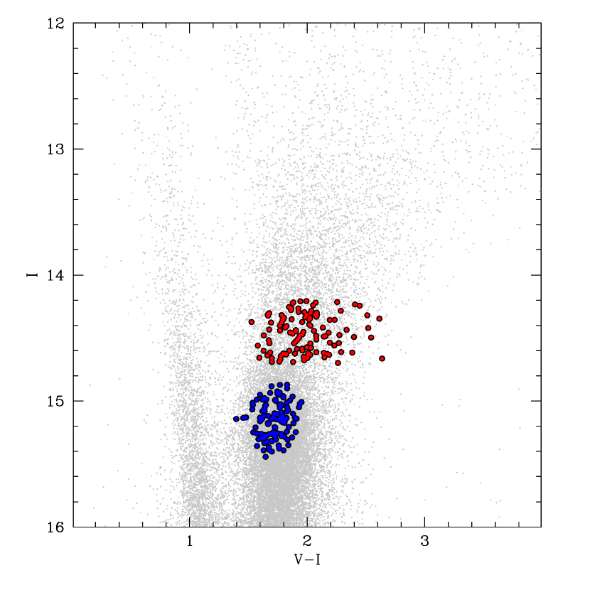
Figure 1: The target selection is shown over the V and I band colour magnitude diagram using color dots. Red and blues correspond to the RC and RGB stars from Baade’s window ($b=-4$).

The target stars we used to construct the CaT calibration are all located in Baade’s Window, and they consist of two samples: 80 stars in the bulge RC, and 68 stars on the RGB, $\sim$0.7 mag brigther than the RC. The medium resolution spectra analysed here were taken with the FLAMES-GIRAFFE multifibre spectrograph at the VLT, in Medusa mode, within the ESO program ID 385.B-0735(B). The spectrograph allows us to obtain spectra for $\sim$130 objects, including sky positions, over a 25 arcmin diameter field of view. We selected the LR08 setup, which covers the wavelength range between 8206 and 9400 Å, with a spectral resolution of $\rm R\approx 6500$. The exposure time needed to reach a mean signal to noise of $\sim 50$/pix were 900 and 1800 seconds for RGB and RC stars, respectively.

High resolution spectra for the targets in Baade’s Window were obtained from Zoccali et al. (2008) and Hill et al. (2011) who used the same instrument in the setups HR13 and HR14, at resolution $\rm R\approx 22,500$ and $\rm R\approx 28,800$, respectively. Figure 1 shows the corresponding color magnitude diagrams (CMDs) for the target selection.

The data reduction was done using the instrument pipeline provided by ESO (version 2.8), which performs bias, flat field corrections, wavelength calibration, and 1-D extraction based on the daytime calibration images. Since the pipeline does not include the sky subtraction routine, we performed this task with IRAF as follows. As a first step, a master sky spectrum was created by combining all the sky spectra ($\sim 20$ per setup) using the median and a sigma clipping algorithm. Figure 2 (upper panel) shows the raw spectrum of a typical star, around the CaT region, together with the master sky spectrum for the same exposure. It is clear that the three CaT lines do not suffer from strong contamination from sky emission lines compared with CaT line strength. The master sky spectrum was then subtracted from each individual science spectrum using the IRAF task skytweak. The latter allows shifting and scaling of the master sky spectrum until a good subtraction is achieved. In order to find the best shift and scale factor we used the strong emission lines located in the wavelength range between 8261 to 8481 Å  and 8739 to 9071 Å.

The spectra were normalized with the IRAF task continuum, using the wavelength range between 8250-8461 Å, 8568-8650 Å, and 8700-9273 Å, in order to avoid the CaT lines. Finally, radial velocities were measured by means of cross-correlation (fxcor task) against a template synthetic spectrum for a typical metal poor K giant star ($T_{\rm eff}=4750$, $\log\;g=2.5$ and $\rm[Fe/H]=-1.3$). Such low metallicity was chosen in order to ensure that the CaT lines in the template were relatively deep but free from contaminations by other lines on their wings.

Example of the final spectra, sky subtracted, radial velocity corrected and continuum normalized are shown in the lower panel of Fig. 2, for stars of different metallicities. An arbitrary shift has been applied along the y-axis, to avoid overlaps.

3 The Calcium Triplet calibration

Figure 2: The upper panel shows the normalized raw spectrum for a typical Milky Way bulge star, together with the corresponding sky spectrum. The lower panel shows processed spectra for 4 bulge stars spanning the typical metallicity range of the Galactic bulge. The increasing strength of the CaT lines with metallicity is evident, together with the increasing number of small atomic lines contaminating the continuum.

The spectral region around the CaT feature (8350-9000 Å) includes several lines which might dominate the spectrum, depending on the spectral type of the star under analysis. Cenarro et al. (2001) showed that stars with spectral type between F5 ($T_{\rm eff}\sim 6500$ K) and M2 ($T_{\rm eff}\sim 3700$ K) are the best targets to measure the CaT lines, due to their only marginal contamination by FeI, MgI and TiI lines. CaT lines in hotter stars are blended with Paschen lines, while in cooler stars the continuum is plagued by TiO molecular bands. Being of K spectral type, our targets are well inside the recommended temperature range.

Additional constraints have been proposed in terms of the brightness range where a single gravity correction can be used (see section 3.2 for details). Carrera et al. (2007) defined a minimum absolute magnitude $M_{V}\leq 1.25$ or $M_{I}\leq 0.0$, while Da Costa et al. (2009) recommends a lower brightness limit of $\sim 0.2$ mag below the RC (or the horizontal branch). Both our RGB and RC targets are inside these constraints, with the RC stars being within the intrinsic dispersion – mainly due to metallicity and distance spread – of the RC in Baade’s Window.

3.1 The equivalent width measurements

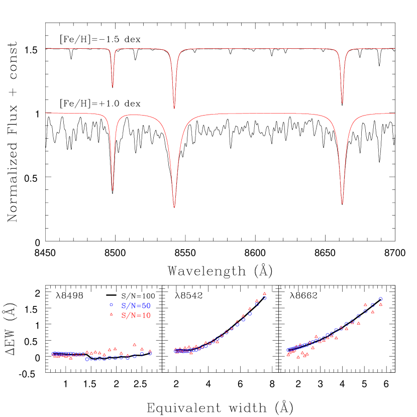
Figure 3: The upper panel shows for comparison the more metal poor and metal rich synthetic spectra from our library, in the region around the CaT lines. In both cases, the black line shows the spectra including the lines of all elements, while the red lines shows only the three CaT lines. The lower panels show the difference between the real EW, as measured in the red spectra, and the measured EW, as measured in the black spectra, for each of the three CaT lines, as a function of EW and for three values of S/N.

While both our RC and RGB target stars are inside the recommended temperature and gravity range for CaT measurements, the metallicity distribution of the Galactic bulge reaches (extends) to significantly higher metallicity than typical star clusters for which this calibration has been defined and used so far. The impact of the metal content over the CaT EWs measurements is mostly driven by the continuum depletion due to the increasing contamination of the CaT lines by other atomic lines. In order to explore the impact of the metal content on the CaT EWs measurement, we analysed a grid of synthetic spectra generated using turbospectrum. The latter is a code of line synthesis described in Alvarez & Plez (1998) and improved along the years by B. Plez. In this case it was used together with the grid of OSMARCS spherical model atmospheres (Gustafsson et al. 2008). The synthetic spectra have the same resolution as the GIRAFFE spectra, and a set of stellar parameters representative of a K giant star ($T_{\rm eff}=4750$ and $\log\;g=2.5$). Only the metallicity was allowed to vary across the range from [Fe/H]=$-1.5$ to the extreme case of [Fe/H]=+1.0 dex, keeping [Ca/H]=[Fe/H] in the whole grid.

Synthetic spectra for stars at the two extreme ends of the metallicity grid are plotted in the upper panel of Fig.3. The black line is the synthetic spectrum containing list of all the element in the wavelength range between 8450 and 8700 Å. The red line, in contrast, shows only the three CaT lines. This exercise clearly shows the depletion of the continuum (pseudo-continuum), at high metallicity, due to the presence of many unresolved lines. Because we deal with normalized spectra (without flux calibration) we need to include the effect of continuum depletion in the empirical calibration itself.

The measurements of the CaT EWs can be done by fitting an empirical function to each line profile and calculate the corresponding EW from direct integration of the function. Different functions have been explored over the years. Armandroff & Da Costa (1991) used a Gaussian profile, when fitting stars in globular clusters. Rutledge et al. (1997), instead, used a Moffat function. Both functions give good results only for stars of relatively low metallicity. In fact, Cole et al. (2004) showed that in the metal rich regime, the strong wings of the CaT lines can be reproduced by the sum of a Gaussian component, fitting the line core, and a Lorentzian function, fitting the wings. Erdelyi-Mendes & Barbuy (1991) and Battaglia et al. (2008) showed that the EWs of CaT lines is driven mostly by the wings, because of the strong pressure broadening. In other words, the strength of the line is mostly driven by the electronic pressure (i.e., metallicity), rather than by the usual combination of temperature and elemental abundance, shaping weak lines.

Table 1:

Feature (Å)	Line bandpass (Å)
8498.02	8491.02 – 8505.02
8542.09	8530.09 – 8554.09
8662.14	8653.14 – 8671.14

In order to test the accuracy of the Gaussian+Lorentzian fit across a range of metallicity and signal to noise, we performed some measurements on the grid of synthetic spectra described above. As a first step, EWs were measured in the synthetic spectra containing only Calcium lines by means of numerical integration. These were assumed to be the real EWs. As a second step, the grid of synthetic spectra was convolved to the resolution and resampled in wavelength to match real data and degraded to different S/N, from 10 to 100 in steps of 10. A Poisson noise model was used for the last operation. The resulting spectrum was then re-normalized to a pseudo-continuum of 1, and the combination of a Gaussian and a Lorentzian function was fitted to the CaT lines. The wavelength ranges used by Armandroff & Zinn (1988) for the fit were slightly modified, as listed in Table 1, in order to improve the fit of the wings. The lower panel of Fig. 3 shows the difference between the measured and the real EWs, for each of the CaT lines, as a function of EW (metallicity) and S/N. It is clear that the EWs of the two strong lines would be underestimated in the data, and more so at high metallicities. This systematic reaches up to $\sim$1 Å  around [Fe/H]=+0.5. However, the trend is very smooth and it is not affected by S/N, down to a S/N$\sim$10, much lower than our poorest spectrum. As a consequence, a correction for this systematic will be implicitly included in the [Fe/H]-vs-CaT empirical calibration equation derived in Section 3.4. For the weakest line, the systematic difference between real and measured EW is much smaller than for the strong lines. However, a step is found around EW${}_{1}=1.5$ Å, due to the appearance of some blends in the wings of this line. Additionally, the weakest line is the most affected by unperfect sky subtraction, due to the presence of two sky lines close to its wings. For this reason, we discarded this line in the following analysis.

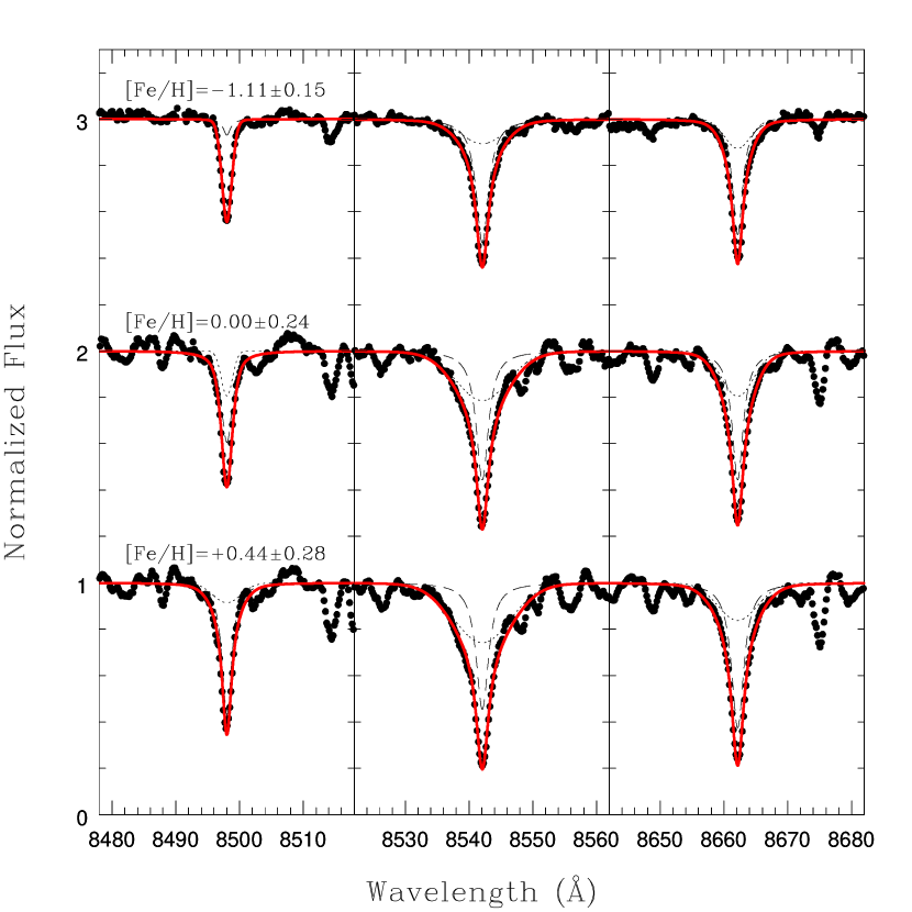
Figure 4: Fitting examples for three bulge stars covering the metallicity range of the Milky Way bulge. The red line correspond to the best fitting function found for each line, while as dashed lines are plotted the individual contribution from Gaussian and Lorentzian functions.

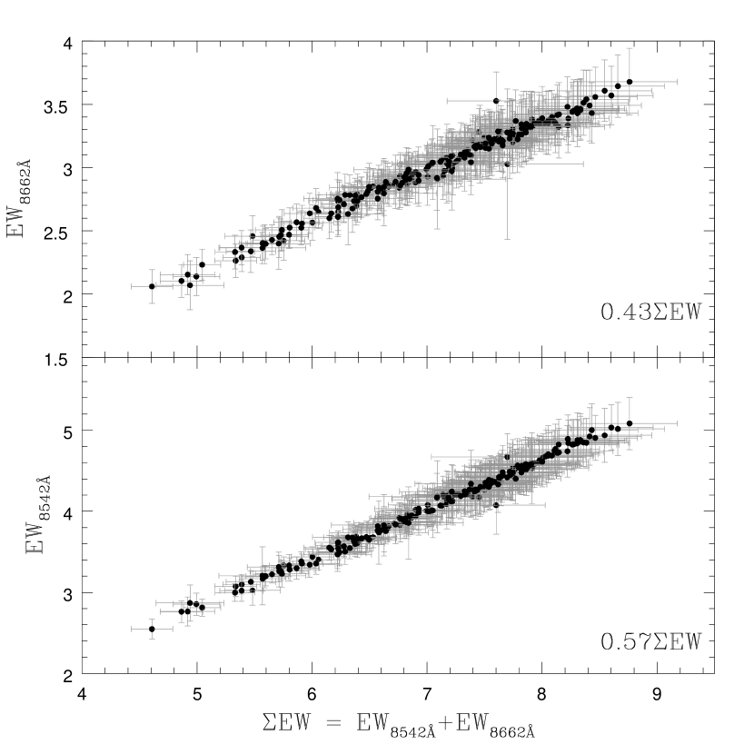
Figure 5: The strength of the two strongest CaT lines versus the sum of the two lines, $\Sigma\leavevmode\nobreak\ EW$. The corresponding fractional contribution with respect to $\Sigma\leavevmode\nobreak\ EW$ is shown in each panel.

Figure 6: Comparison between our measurements and the literature values of the sum of the two strongest lines for different stellar cluster taken from Warren & Cole (2009) and Saviane et al. (2012).

Examples of line fitting are shown in Fig. 4 for three observed spectra covering the metallicity range of the Milky Way bulge. For each star, the big black dots show the observed spectrum, the red line is the final fit, while the thin dotted and dashed lines show the individual contribution of the Gaussian and the Lorentzian profiles, respectively. Additionally, the line-ratio between the two strongest CaT lines is remarkably constant across the metallicity range spanned by the bulge data. Figure 5 shows the contribution of the two strongest individual CaT lines to the sum of the two. The data can be fitted by a single line, with the slope indicated in the label. This line ratio can be used, for instance, to predict the EW of one of the lines, when the other is not available for a direct measurement. It can also be used to test the consistency of the measurements, in order to reject lines with anomalous line ratio. This is particularly useful when dealing with large surveys.

As will be explained in the following sections, we will use cluster stars to constrain the final metallicity CaT calibration. Before doing it, we need to verify that our EWs measurements are in the same scale as those used in previous works. To this end, we obtained the spectra of the two most metal rich clusters (NGC 6791 and NGC 6819) in the sample by Warren & Cole (2009) and re-measure EWs. The spectra kindly provided to us, by private communication, were already wave-calibrated and sky-subtracted, therefore we only applied the same continuum normalization procedure and EW measurement used for our data. Additionally, in order to to probe a wider range of metallicity, we also measured a sample of globular cluster stars, drawn from Saviane et al. (2012), spanning the metallicity range $-2.3<$[Fe/H]$<+0.07$. The selected stars belong to the globular clusters M 15, NGC 6397, M4, NGC 6553, and NGC 6528. Figure 6 shows the excellent agreement between our measurements and the literature one, for the sum of the EWs of the two strongest CaT lines, hereafter $\rm\Sigma EW$ ($=EW_{8542}+EW_{8662}$).

3.2 The reduced equivalent width

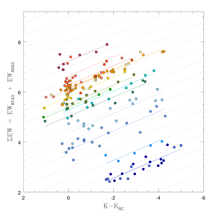
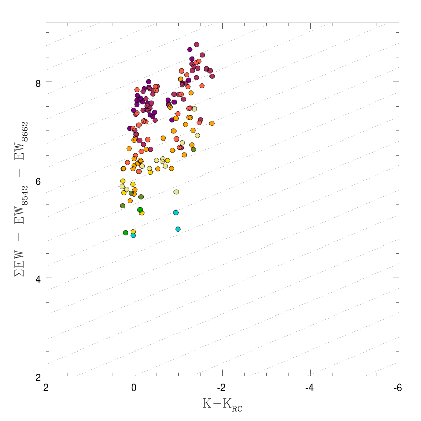
Figure 7: The CaT equivalent widths of the star cluster RGBs (left panel) and Galactic bulge stars (right panel) are compared with their corresponding magnitude above the mean red clump magnitude. The colour code is used to mark clusters of different metallicity, together with their best-fitting lines, assuming the best common slope of $0.384$ Åm̃ag^-1. Thin dotted lines in each panel show this slope, to guide the eye.

The strength of an atomic line, in general, is driven by the elemental abundance, the effective temperature, and the surface gravity of the star. Both Armandroff & Da Costa (1991) and Olszewski et al. (1991) showed that the combined effect of effective temperature and surface gravity on the EWs of CaT lines can be parametrized as a function of luminosity alone. The CaT EWs corrected by this effect (i.e., the reduced EWs) depend only upon metallicity. Specifically, they found that, in each given cluster, red giant stars follow a straight line in the luminosity-$\rm\Sigma EW$ plane. The slope of the line is identical for different clusters, while its zero point depends on the cluster metallicity. As a proxy for luminosity, some authors use the absolute magnitude of the star (Carrera et al. 2007, 2013), or, most commonly, the difference between the star apparent magnitude and the magnitude of the cluster horizontal branch, or red clump (Armandroff & Da Costa 1991; Rutledge et al. 1997; Cole et al. 2004; Battaglia et al. 2008; Warren & Cole 2009; Saviane et al. 2012; Mauro et al. 2014). We adopted the second option, in order to minimize the uncertainty in the distance and reddening, both variable across the Galactic bulge.

The $K_{s}$ magnitude, from the VVV survey (Minniti et al. 2010), was used for our bulge stars. In order to determine the slope in the luminosity-$\rm\Sigma EW$ plane we used the star cluster data from Warren & Cole (2009). For each cluster star we plot $\rm\Sigma EW$ as a function of $(K-K_{\rm RC})$ and fit a linear relation, deriving a representative slope by making the average of the single measurements. The left panel of Fig. 7 shows the straight lines defined by different clusters, each in a different color. They are consistent with a constant slope of $\beta_{K_{s}}=0.384\pm 0.019$ Å  mag^-1, in excellent agreement with those derived by Mauro et al. (2014) using the clusters from Saviane et al. (2012) combined with VVV photometry. This slope allows us to define the reduced EW parameter

$$W^{\prime}=\Sigma\mathrm{EW}+\beta_{K_{s}}(K-K_{\rm RC})$$

which is dependent only upon the metallicity of the star.

In order to determine the corresponding $(K-K_{\rm RC})$ for our bulge stars we measure the mean RC magnitude from the complete VVV de-reddened $K_{s}$ photometric catalogue corresponding to the observed field, by using the reddening map presented in Gonzalez et al. (2011c). The right panel of Fig. 7 shows the location of our RC and RGB targets, all in Baade’s Window, in the same plane. The color coding traces metallicity (as measured from the HR spectra), and it is the same used for the star clusters. Contrary to what happens in star clusters, bulge stars in each metallicity bin do not seem to define parallel straight lines. We interpret this as the result of the probable disk contamination, the errorbar on the metallicity of each star, and the intrinsic width of the metallicity bin. Also, while for star clusters the x-axis is a clean proxy for luminosity, bulge stars have a significant distance spread, and the red clump only reflects their mean distance.

3.3 Reference metallicities: Galactic bulge and globular clusters

In order to derive an equation converting between $W^{\prime}$ and the [Fe/H] abundances, a set of independent determinations of [Fe/H] from high resolution spectra are needed. In what follows we describe how those were obtained, both for bulge field giants and for a subset of the globular clusters presented in Warren & Cole (2009). The latter have been added to our sample, after showing that they were fully compatible, in order to extend the metallicity range on the metal poor side.

3.3.1 Homogeneous high resolution metallicities determination for Galactic bulge stars

[Fe/H] abundances for both RC and RGB stars in Baade’s Window, were discussed in Zoccali et al. (2008) and Hill et al. (2011). They were based on GIRAFFE spectra, through setups HR13 and HR14, at resolution R$\sim$22,500 and $\sim$28,800, respectively. After the pre-reduction and coaddition of the spectra explained in Section 2, iron abundances were measured by means of individual, unblended iron lines. Conceptually, we used the same method explained in our previous works, cited above. Namely, first guess effective temperature and gravity were derived from photometry, and used to construct an approximate model atmosphere. The latter was used to derive [Fe/H] abundances, independently, from several FeI and FeII lines. The stellar surface parameters (T_eff, log $g$ and the microturbulent velocity $\chi$) were then refined by imposing consistency among the abundances derived from different lines. As discussed in Hill et al. (2011), the actual implementation of this method may yield slightly different final abundances -especially for metal rich, cold giants- depending on which of the stellar parameters is fixed first. In other words, there can be degeneracies in the parameter space, due to correlations among the stellar parameters.

In order to minimize this effect, for the present work we applied an automated procedure, based on the use of GALA (Mucciarelli et al. 2013). This code is designed to impose the excitation and ionization equilibria on FeI lines, thus deriving T_eff and log $g$, respectively, and to converge on a value for the microtubulent velocity that yields the same [Fe/H] abundance for lines of different EWs. The ATLAS9 (Castelli & Kurucz 2004) model atmosphere were used instead of the MARCS ones (Gustafsson et al. 2008) because GALA is optimized for the former. The results are fully compatible with those of Zoccali et al. (2008) and Gonzalez et al. (2011c). A small offset -within the errorbars- is present between the resulting metallicities and those presented by Hill et al. (2011). The use of GALA, however, does reduce at least the statistical errors, as demonstrated by the exceptionally small spread of abundances in the [Mg/Fe] versus [Fe/H] plot, presented in Zoccali et al. (2015) and Gonzalez et al. (2015, in preparation).

3.3.2 Globular clusters

In order to constrain the CaT versus [Fe/H] calibration in the metal poor regime, where bulge stars are sparse, we considered adding to our sample some globular clusters. A natural choice was a subset of the Warren & Cole (2009) cluster sample. This is for two main reasons: i) we had access to their spectra, and indeed we have shown in Fig. 6 that the EWs measured with our method is fully consistent with theirs; and ii) $K_{s}$ photometry is available for all those stars. In their work, Warren & Cole (2009) derived a calibration equation between the CaT reduced EWs, as derived using the three lines, and [Fe/H] measured in the scale of Carretta & Gratton (1997). The latter scale, however, has been revised in Carretta et al. (2009) (hereafter C09), to what has now become a new standard (e.g. Harris 1996, 2010 edition). We therefore updated the [Fe/H] abundances to the C09 scale using the compilation in Carrera et al. (2013). For globular clusters without new [Fe/H] measurements, we used instead the relation provided in C09, to transform the metallicity from the old to the new scale. It is worth emphasizing here that both globular clusters and bulge stars have the same calcium over iron ratio ([Ca/Fe]$\sim$+0.4) at [Fe/H]$\sim-1$ where they overlap (Gonzalez et al. 2011a; Carrera et al. 2013).

The calibration by Warren & Cole (2009) includes several open clusters, constraining the metal rich regime. We excluded those from our analysis, because we sample the metal rich side with a large number of bulge stars, and our goal is to optimize the calibration for bulge-like giants. In section 4 we will compare our calibration with open and globular clustr data.

3.4 The metallicity calibration

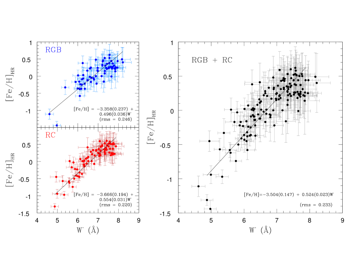
Figure 8: High resolution metallicities are compared with reduced equivalent widths of RGB (blue), RC (red) and the combination of the two (black) bulge star samples. The best fitting CaT calibration for each sample is also shown in each panel.

The calibration equation between $W^{\prime}$ and [Fe/H]_HR was derived by means of an error-weighed least square fitting of the data points relative to individual stars, both in the bulge and in globular clusters. This is different from what is usually done for star clusters, where the mean values of $\left\langle W^{\prime}\right\rangle$ and $\left\langle\rm[Fe/H]\right\rangle$ for each cluster are used. Several fitting functions were tested before concluding that a linear relation was the best choice, because it minimizes the artificial saturation of the calibration equation at high metallicity (i. e. a constant metallicity at higher $W^{\prime}$). The latter, indeed, may create an unphysically sharp cut-off in the iron distribution function.

As a first step, a linear fitting was performed between $W^{\prime}$ and [Fe/H]_HR for RGB and RC stars, independently. The results are shown in the left panels of Fig. 8, together with the rms ($\sim$0.23) which is comparable to the uncertainties of the [Fe/H]_HR measurements. The fits are consistent with each other, and can therefore be combined in the single linear relation shown in the right panel of the same figure, namely:

$$\mathrm{[Fe/H]_{RGB+RC}}=(-3.504\pm 0.147)+(0.524\pm 0.023)W^{\prime}$$ (1)

whith a rms of $0.233$ dex.

As a second step, 7 globular clusters were added to the plot, covering the metallicity range $-2.3<$[Fe/H]$<-0.7$. The fit of a linear relation between the mean $W^{\prime}$ and mean [Fe/H], for the clusters only, yields:

$$\mathrm{[Fe/H]_{GC}}=(-3.175\pm 0.094)+(0.462\pm 0.025)W^{\prime}$$ (2)

which, though slightly different from the equation found for the bulge (Eq. 1), shows a smooth transition between the two when they overlap. This suggests that a single calibration can be used, valid across the whole range $-2.3<$[Fe/H]$<+0.7$. Nevertheless, as globular cluster and Galactic bulge stars do not have the same data sampling (i.e. for globular clusters $\left\langle W^{\prime}\right\rangle$ and $<$[Fe/H]${}_{\rm HR}>$ are used instead of the measurements for individual stars) we cannot directly combine the data sets in order to fit a single function, because the resulting fit would be dominated by the metal poor data, having smaller errors in [Fe/H]. Because of this, we decided to create two evenly sampled fiducial data sets taken from the equations (1) and (2), in the $W^{\prime}$ range between $0<W^{\prime}<5.4$ and $5.2<W^{\prime}<10$ respectively. These data sets were then combined into a single one and fitted by a second order function in order to take into account the small change of slope between the two linear equations (Eq. 1 and 2).

The resulting fit gives:

$$\mathrm{[Fe/H]_{CaT}}=-3.150+0.432W^{\prime}+0.006W^{\prime 2}$$ (3)

with a rms dispersion around the fit of $0.197$ dex. No errors are quoted for the coefficients here, because, due to the procedure adopted to combine globular clusters and bulge stars, this is more a fiducial relation, characterizing the locus of the data in the $W^{\prime}$ versus [Fe/H] plane, rather than a formal fit.

When applying the calibration, errors on the derived [Fe/H] values will be calculated as the quadratic sum of the errors on the EW, propagated through equation 3, and the rms of the same equation. Figure 9 summarizes our results, showing the final CaT vs [Fe/H] calibration, as a green line, together with the bulge stars (black dots) and the globular clusters (orange dots). For the latter, individual $W^{\prime}$ -measured by Warren & Cole (2009)- are plotted for individual stars, all at the same cluster $<$[Fe/H]_HR. The upper-left corner shows the histogram of the residuals for bulge stars, i.e., the differences between [Fe/H]_HR and [Fe/H]_CaT. The distribution is symmetric around zero and the dispersion is consistent with the rms quoted above.

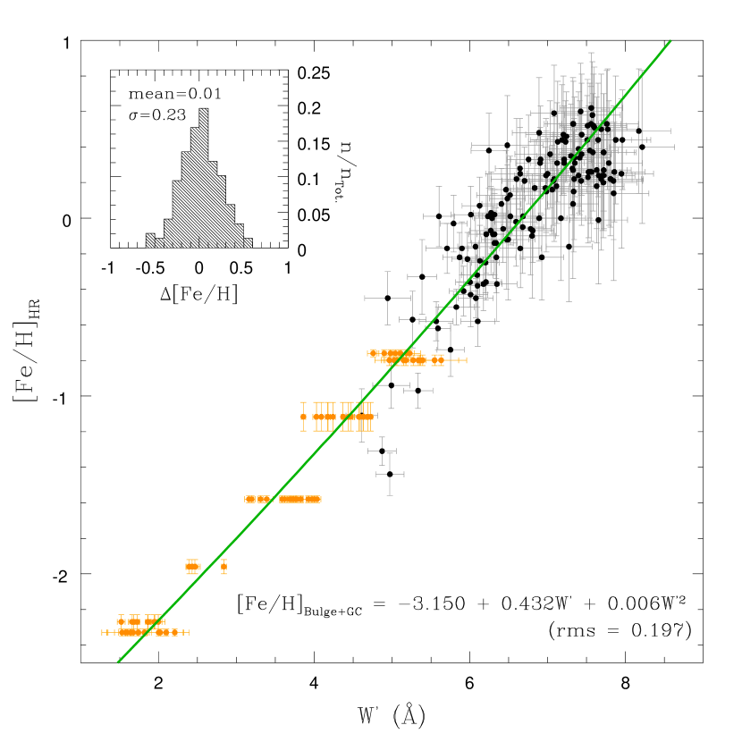
Figure 9: The CaT calibration for the combination between bulge stars (black) with globular clusters from Warren & Cole (2009) (orange). The upper left panel shows the corresponding calibration metallicity residuals for bulge stars.

4 Comparison with previous calibrations

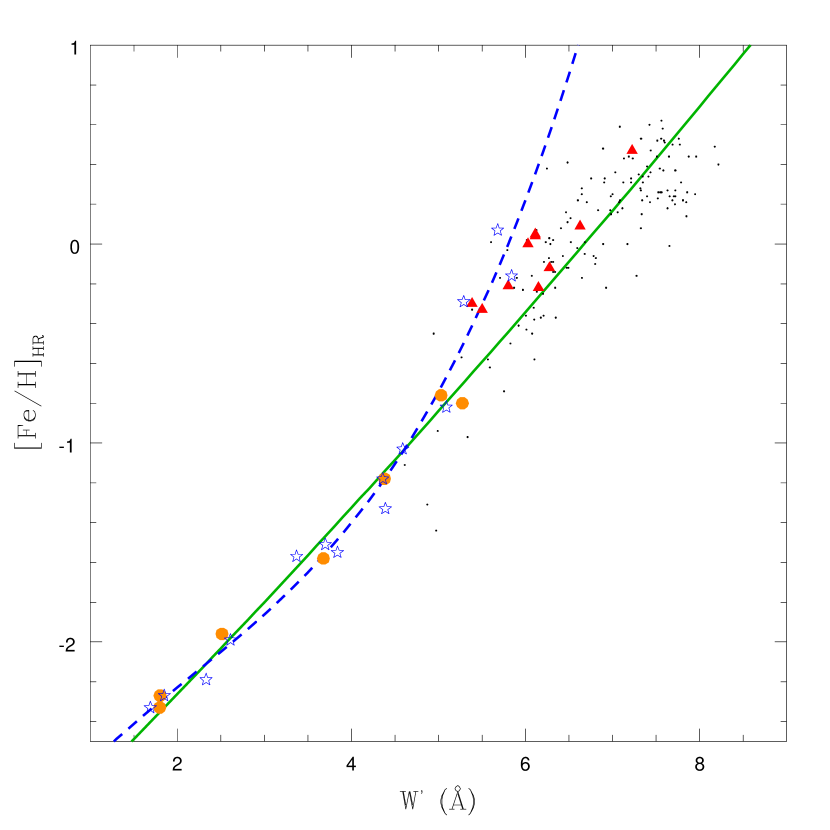
Figure 10: High resolution metallicity versus the reduced equivalent width for different star samples: bulge stars (black dots), globular (orange circles) and open (red triangles) clusters from Warren & Cole (2009), and globular clusters (blue stars) from Saviane et al. (Saviane et al. 2012). Our CaT calibration is plotted as a green line, while the cubic calibration from Saviane et al. (2012) is the dashed blue line.

Different CaT vs [Fe/H] calibration have been proposed in the past, differing among each others mainly because of the different methods to measure EWs, and the different [Fe/H] scales. A recent calibration is presented in Saviane et al. (2012) who used 14 globular clusters to define a cubic equation covering the range $-2.33<$[Fe/H]$<0.07$, in the C09 scale. Since the EWs measured by us are fully compatible with the Saviane et al. (2012) (c.f., Fig. 6), the two calibrations can also be directly compared.

Figure 10 is color coded as Fig. 9, with bulge giants as small black dots and globular and open cluster mean values as orange and red dots, respectively (Warren & Cole 2009). Our calibration is shown as a green line. Also shown are the globular clusters in (Saviane et al. 2012, blue stars) and their calibration equation, as a blue dashed line. The two calibrations, as well as the original one from Warren & Cole (2009), are consistent with each other for [Fe/H]$<-0.8$ dex. The higher order fit in Saviane et al. (2012) is required only by the three most metal rich globular clusters in their study, namely: NGC 5927 ([Fe/H]=$-0.29$), NGC 6553 ([Fe/H]=$-0.16$) and NGC 6528 ([Fe/H]=$+0.07$). Interestingly, the same behaviour is seen in C09, where the updated Rutledge et al. (1997) calibration changes from a linear to a cubic fit when NGC 6553 is added to the original sample (see Fig. A.2 from Carretta et al. (2009)). Moreover, as noted by Saviane et al., NGC 6528 has $W^{\prime}$ lower than NGC 6553, though being more metal rich.

Although we are not able to explain the difference between the three most metal rich globular clusters and bulge stars, we note that the cubic relation of Saviane et al. (2012) is clearly not appropriate for bulge stars, which are the main focus of our interest. Also shown in Fig. 10 are the open clusters from Warren & Cole (2009). Although the authors originally derived a linear calibration, the use of the updated [Fe/H] from Carrera et al. (2013) for the open clusters is not compatible anymore with a single straight line. The difference between orange dots and red triangles, in Fig. 10, looks more like a systematic shift, rather than a change of slope. A similar shift can be observed in the [Ca/H] versus [Fe/H] plot shown in Fig. 11 of Carrera et al. (2013), and it might be ascribed to inhomogeneities in the [Fe/H] sources for open clusters, or to a systematic effect due to age, compared to globular clusters.

5 Conclusions

Using RGB and RC stars from Baade’s window we have constructed a CaT versus [Fe/H] calibration, valid in the metal rich regime up to [Fe/H]=+0.7. Since bulge stars are rather sparse for [Fe/H]$<-0.5$, we used globular clusters to constrain the behaviour of the calibration relation in the metal poor regime. We found that a single linear relation can be fitted across the whole range $-2.3<$[Fe/H]$<+0.7$. A minor second order deviation from a single linear relation, however, gives a better fit, properly taking into account the small difference between the linear best fit for globular clusters (equation 1) and for bulge giants (equation 2). It is worth emphasizing that both globular clusters and bulge stars have [Ca/Fe]$\sim+0.3$ in the common metallicity range, therefore a possible dependence of the calibration upon the [Ca/Fe] ratio would not affect the combination of the two datasets. At higher metallicities the bulge [Ca/Fe] drops to zero (Gonzalez et al. 2011b, 2015) but the CaT-vs-Fe calibration found here is still almost linear, possibly due to the combined effect of the strong saturation of CaT lines. The new calibration, represented by equation 3, allows one to derive the iron content of metal rich stars by means of low-resolution spectra. The latter are the only viable way to sample a large number of stars in high extinction regions, such as the Galactic bulge, or, in the future, in metal rich external spheroid such as the inner halo of M31.