A practical parametrization for line shapes of near-threshold states

Abstract

Numerous quarkonium(like) states lying near $S$-wave thresholds are observed experimentally.We propose a self-consistent approach to these near-threshold states compatible with unitarity and analyticity.The underlying coupled-channel system includes a bare pole and an arbitrary number of elastic and inelastic channels treated fully nonperturbatively.The resulting analytical parametrization is ideally suited for a combined analysis of the data available in various channels that is exemplified by an excellent overall description of the data for the charged $Z_{b}(10610)$ and $Z_{b}(10650)$ states.

I Introduction

At present there is no doubt that QCD is the true theory of strong interactions, at least at the energy scale presently accessible for experimental investigations. One of the remarkable features of QCD is the prediction of the existence of multiconstituent states, with a structure more complex than just quark-antiquark or three-quark configurations, which are conventionally referred to as “exotic” hadrons. Experimental searches and theoretical studies of such exotic states constitute an important tool in investigations of nature. Since the discovery of the charmonium(like) state $X(3872)$ in 2003 Choi:2003ue , numerous experiments continue to deliver intriguing data on other charmonium(like) and bottomonium(like) states lying above the respective open-flavor thresholds. Although for most of these states it is not possible at present to make definite conclusions concerning their nature, some of these states share an important feature, namely they reside in the vicinity of strong $S$-wave thresholds and they are seen in both open-flavor (elastic) and hidden-flavor (inelastic) final states. Paradigmatic examples of such states are the $X(3872)$ near the $D^{0}\bar{D}^{*0}$ threshold, the $Z_{b}(10610)$ and $Z_{b}(10650)$ near the $B^{(*)}\bar{B}^{*}$ thresholds, and the $Z_{c}(3900)$ and $Z_{c}(4020)/Z_{c}(4025)$ near the $D^{(*)}\bar{D}^{*}$ thresholds. Since vast and detailed information is becoming available from existing experiments, and even more precise data are expected from future high-statistics and high-precision experiments Abe:2010gxa ; Drutskoy:2012gt ; Asner:2008nq ; Lutz:2009ff for states that are already known (see Brambilla:2010cs ; Brambilla:2014jmp for recent reviews) as well as for ones that are new and as yet unobserved, adequate theoretical tools for the data analysis are urgently called for. The aim of this Letter is to propose such a tool that is especially useful in describing near-threshold phenomena.

The traditional way to perform an analysis of the experimental data is by using of individual Breit-Wigner distributions for each peak combined with suitable background functions. However, such an approach provides only limited information on the states studied, since the Breit-Wigner parameters are reaction-dependent and the naive algebraic sum of the Breit-Wigner distributions violates unitary. In addition, by analyzing each reaction channel individually, one does not exploit the full information content provided by the measurements. The approach proposed in this Letter provides an important link between various models and first-principles calculations in QCD (for example, lattice simulations) from one side to the experimental data on the other side. To this end, we build a model-independent parametrization for near-threshold phenomena consistent with requirements from unitarity and analyticity. The formulas derived allow one to perform a simultaneous analysis of the entire bulk of data for all decay channels for given near-threshold states(s). The resulting parametrization includes in a fully nonperturbative way a bare pole and an arbitrary number of elastic and inelastic channels. With the help of not-very-restrictive and phenomenologically justifiable assumptions the formulas can be solved analytically, which makes them as ideal for data analysis. The parameters of the final expressions are renormalized quantities with a direct physical meaning. The suggested parametrization is, therefore, expected to have a broad impact on the analysis of experimental data and to provide important insights into the phenomenology of the strong interactions.

II Parametrization for the line shapes

We consider a coupled-channel approach based on the Lippmann-Schwinger equation (LSE) for the $t$ matrix $t$,

$$t=\hat{V}-\hat{V}St,$$ (1)

where $S$ denotes the free propagator in the corresponding channel. The potential

$$\hat{V}= \scriptstyle\mbox{\scriptsize Pole}\hskip 19.91692pt\beta=\overline{1,N_{e}}\hskip 19.91692pti=\overline{1,N_{in}} \begin{pmatrix}0&f_{\beta}({\bm{p}}^{\prime})&f_{i}({\bm{k}})\\[5.69054pt] f_{\alpha}({\bm{p}})~{}&~{}v_{\alpha\beta}({\bm{p}},{\bm{p}}^{\prime})~{}&~{}v_{\alpha i}({\bm{p}},{\bm{k}})\\[5.69054pt] f_{j}({\bm{k}}^{\prime})&v_{j\beta}({\bm{k}}^{\prime},{\bm{p}}^{\prime})&v_{ji}({\bm{k}}^{\prime},{\bm{k}})\end{pmatrix} \alpha=\overline{1,N_{e}} j=\overline{1,N_{in}}$$

Pole

.

contains all possible types of interaction between the bare pole (labeled as “0”—for example, its position is $M_{0}$), the set of $N_{e}$ elastic open-flavor channels $(Q\bar{q})(q\bar{Q})$ (here $Q$ and $q$ denote a heavy and a light quark, respectively) labeled by Greek letters, and a set of $N_{in}$ inelastic hidden-flavor channels $(Q\bar{Q})(q\bar{q})$ referred to by Latin letters.

In order to proceed with the analytic solution, we make a few simplifying assumptions. In general there are good reasons to neglect the direct interactions in the inelastic channels. For example, for the $X(3872)$ transitions between the $\rho J/\psi$ and $\omega J/\psi$ channels are forbidden by the isospin conservation. In addition, since there are no light quarks inside the $J/\psi$ state, the direct potential for $\rho(\omega)J/\psi\to\rho(\omega)J/\psi$ is also expected to be weak. Analogously, since there are no light quarks in the heavy quarkonia $\Upsilon(nS)$ and $h_{b}(mP)$, their interaction with pions is expected to be weak, with obvious relevance for the $Z_{b}^{(\prime)}$ states. Indeed, effective field theory estimates Liu:2012dv and lattice calculations Detmold:2012pi give very small values for the scattering lengths of the pion scattered off the $c\bar{c}$ and $b\bar{b}$ quarkonia. We therefore set $v_{ji}({\bm{k}}^{\prime},{\bm{k}})=0$. Next, we assume a separable form of the elastic transition vertex, $v_{\alpha i}({\bm{p}},{\bm{k}})=\chi_{\alpha}({\bm{p}})\varphi_{i\alpha}({\bm{k}})$, where the additional assumption was made that $\chi_{i\alpha}$ is independent of $i$. Indeed, the transition of the open-flavor channels to the hidden-flavor channels demands the exchange of a heavy meson and, therefore, it is necessarily of short range for all inelastic channels. Without loss of generality we set $\chi_{\alpha}({\bm{p}}=0)=1$. In addition, in a relatively narrow region near the elastic threshold(s) it is sufficient to parametrize the transition form factors as

$$f_{\alpha}({\bm{p}})=f_{\alpha},\chi_{\alpha}({\bm{p}})=1,\varphi_{i\alpha}({\bm{k}})=g_{i\alpha}|{\bm{k}}|^{l_{i}},f_{i}({\bm{k}})=\lambda_{i}|{\bm{k}}|^{l_{i}},$$

where $f_{\alpha}$, $g_{i\alpha}$, $\lambda_{i}$ are constants and $l_{i}$ is the angular momentum in the $i$th channel. The elastic potential, $v_{\alpha\beta}$, is approximated by a constant matrix.

The omission of rescatterings within the inelastic channels allows us to disentangle the latter from the elastic channels and from the pole term. We define the potentials

$$V_{00}=-\sum_{i}\raisebox{-7.68222pt}{\psfig{width=45.5244pt}}=-\sum_{i}\lambda_{i}^{2}J_{i},$$

$$V_{\alpha 0}=\raisebox{-8.53581pt}{\psfig{width=25.60747pt}}-\sum_{i}\raisebox{-7.68222pt}{\psfig{width=45.5244pt}}=f_{\alpha}-\sum_{i}g_{i\alpha}J_{i}\lambda_{i},$$

$$V_{0\beta}=\raisebox{-8.53581pt}{\psfig{width=25.60747pt}}-\sum_{i}\raisebox{-7.68222pt}{\psfig{width=45.5244pt}}=f_{\beta}-\sum_{i}\lambda_{i}J_{i}g_{i\beta}$$

$$V_{\alpha\beta}=\raisebox{-5.97508pt}{\psfig{width=19.91692pt}}-\sum_{i}\raisebox{-8.53581pt}{\psfig{width=48.36967pt}}=v_{\alpha\beta}-\sum_{i}g_{i\alpha}J_{i}g_{i\beta},$$

where the thin solid lines, broad solid lines and dashed lines denote heavy-light mesons, heavy mesons, and light mesons, respectively, and the double line denotes the pole term. The inelastic loop integral is

$$J_{i}=\int|{\bm{q}}|^{2l_{i}}S_{i}({\bm{q}})d^{3}q\to\frac{i(2\pi)^{2}}{\sqrt{s}}m_{th_{i}^{in}}\mu_{i}^{in}(k_{i}^{in})^{2l_{i}+1},$$ (3)

where the real part is omitted since it only renormalizes parameters of the interaction; $\mu_{i}^{in}$, $k_{i}^{in}$, $m_{th_{i}^{in}}$ are the reduced mass, the relative momentum, and the threshold in the $i$th inelastic channel, respectively. To disentangle the pole term from the elastic channels we define

$$V_{\alpha\beta}^{\rm eff}=v_{\alpha\beta}-G_{\alpha\beta}-V_{\alpha 0}G_{0}V_{0\beta},~{}\displaystyle V_{\alpha 0}^{\rm eff}=V_{\alpha 0}(1+G_{0}V_{00}),$$

where $G_{0}=1/(M_{0}-M+V_{00}-i0)$ while the inelastic “bubble” operator is

$$G_{\alpha\beta}\equiv\sum_{i}\raisebox{-7.68222pt}{\psfig{width=45.5244pt}}=\sum_{i}g_{i\alpha}J_{i}g_{i\beta}.$$ (4)

We arrive, therefore, at a pair of decoupled LSE

$$t_{\alpha\beta}=V^{\rm eff}_{\alpha\beta}-\sum_{\gamma}V^{\rm eff}_{\alpha\gamma}J_{\gamma}t_{\gamma\beta},~{}t_{\alpha 0}=V^{\rm eff}_{\alpha 0}-\sum_{\beta}V^{\rm eff}_{\alpha\beta}J_{\beta}t_{\beta 0},$$

(5)

$$J_{\alpha}=\int S_{\alpha}({\bm{p}})d^{3}p=(2\pi)^{2}\mu_{\alpha}(\kappa_{\alpha}+ik_{\alpha})\equiv R_{\alpha}+iI_{\alpha},$$

with $\mu_{\alpha}$ and $k_{\alpha}$ being the reduced mass and the relative momentum in the $\alpha$’s elastic channel, respectively, $k_{\alpha}=\sqrt{2\mu_{\alpha}(M-m_{th_{\alpha}})+{i\epsilon}}$, where $m_{th_{\alpha}}$ is the position of the $\alpha$th elastic threshold. We reduced the entire problem to Eqs. (5). Thus, independent of the number of inelastic channels the solution of these implies only the inversion of matrices as small as $N_{e}\times N_{e}$, where typically $N_{e}=2$ (cf. the explicit example below). The transitions to inelastic channels follow from the solutions to Eqs. (5) straightforwardly, without the need to solve another scattering equation. Therefore, the proposed approach drastically simplifies the combined analysis of experimental data. In particular, adding a further inelastic channel changes the final expressions only marginally. Since the approach is based on a LSE, unitarity is preserved automatically and all imaginary parts are linked to observable rates.

In order to solve Eqs. (5) we proceed stepwise, analogous to the two-potential formalism twopotform ; Hanhart:2012wi . Our starting point is a convenient parametrization for $t^{v}$, the solution of the LSE $t^{v}=v-vSt^{v}$, where $v$ is the direct interaction potential in the elastic channels. The coupling to the inelastic channels is then switched on, and a LSE for the potential $w=v-G$, where the matrix $G$ was defined in Eq. (4), is solved with the result

$$t^{w}=t^{v}+\psi[{\cal G}-G^{-1}]^{-1}\bar{\psi},$$ (6)

where the dressed vertices and the matrix ${\cal G}$ are

$$\psi_{\alpha\beta}=\delta_{\alpha\beta}\chi_{\alpha}-t^{v}_{\alpha\beta}J_{\beta},\quad\bar{\psi}_{\alpha\beta}=\delta_{\alpha\beta}\chi_{\alpha}-J_{\alpha}t^{v}_{\alpha\beta},$$

(7)

$${\cal G}_{\alpha\beta}=J_{\alpha}\psi_{\alpha\beta}=\bar{\psi}_{\alpha\beta}J_{\beta}=\delta_{\alpha\beta}J_{\alpha}-J_{\alpha}t^{v}_{\alpha\beta}J_{\beta}.$$

Finally, when the coupling to the pole term is included as well, the formalism of Baru:2010ww ; Hanhart:2011jz can be used to yield

$$t_{\alpha\beta}=t^{w}_{\alpha\beta}+\frac{\phi_{\alpha}\bar{\phi}_{\beta}}{M-M_{0}+{\cal G}_{0}},\quad t_{\alpha 0}=\frac{M-M_{0}}{M-M_{0}+{\cal G}_{0}}\phi_{\alpha},$$

where

$$\phi_{\alpha}=V_{\alpha 0}-\sum_{\beta}t^{w}_{\alpha\beta}J_{\beta}V_{\beta 0},\quad\bar{\phi}_{\alpha}=V_{0\alpha}-\sum_{\beta}V_{0\beta}J_{\beta}t^{w}_{\beta\alpha},$$

$${\cal G}_{0}=\sum_{i}\lambda_{i}^{2}J_{i}+\sum_{\alpha}V_{0\alpha}J_{\alpha}\phi_{\alpha}=\sum_{i}\lambda_{i}^{2}J_{i}+\sum_{\alpha}\bar{\phi}_{\alpha}J_{\alpha}V_{\alpha 0}.$$

The $t$ matrix $t_{\alpha i}$ is fully determined by $t_{\alpha\beta}$ and $t_{\alpha 0}$,

$$t_{\alpha i}=\left(g_{i\alpha}+\frac{t_{\alpha 0}\lambda_{i}}{M-M_{0}}-\sum_{\beta}t_{\alpha\beta}R_{\beta}g_{i\beta}\right)(k_{i}^{in})^{l_{i}}.$$ (8)

Since our knowledge of most resonance properties comes from production experiments, we build the production amplitude in the elastic or inelastic channel $x$ as

$${\cal M}_{x}=-\sum_{\beta}\raisebox{-24.18483pt}{\psfig{width=60.70653pt}}=-\sum_{\beta}{\cal F}_{\beta}J_{\beta}t_{\beta x},$$ (9)

where it was assumed that the production proceeds through the $N_{e}$ pointlike elastic sources ${\cal F}_{\alpha}$. We also assumed that the elastic $t$ matrix possesses poles near threshold(s) and, therefore, the Born term in the elastic amplitude was neglected. The differential production rate can be obtained by integrating the standard expression for the three-body decay Agashe:2014kda in the invariant mass $m_{23}^{2}$, neglecting the FSI with particle 3. Then

$$\frac{d\mbox{Br}_{x}}{dM}=\frac{|{\cal M}_{x}|^{2}p_{3}k_{x}}{32\pi^{3}M_{\rm tot}^{2}\Gamma_{\rm tot}},\quad M\equiv m_{12}=\sqrt{s},$$ (10)

where $k_{x}$ is the c.m. momentum of particles 1 and 2. The allowed parameter range for $M$ is given by $M_{\rm min}=m_{1}+m_{2}$ and $M_{\rm max}=M_{\rm tot}-m_{3}$.

It is convenient to introduce new parameters $\Lambda={\cal F}_{1}^{2}$ and $\xi_{\alpha}={\cal F}_{\alpha}/{\cal F}_{1}$, where the sources ${\cal F}_{\alpha}$ were redefined to absorb the slow function of energy $R_{\alpha}$ and the constant factors from Eq. (10). Since for all elastic channels the range of forces is described by the same physics, it is natural to use $R_{\alpha}=(2\pi)^{2}\mu_{\alpha}\kappa$. Then the elastic and inelastic differential rates

$$\displaystyle\frac{d\mbox{Br}_{\alpha}^{e}}{dM}=\Lambda\Bigl{|}\sum_{\beta}\xi_{\beta}t_{\beta\alpha}\Bigr{|}^{2}p_{3}k_{\alpha},$$ (11)

$${\displaystyle\frac{d\mbox{Br}_{i}^{in}}{dM}=\Lambda\Bigl{|}\sum_{\alpha}\xi_{\alpha}t_{\alpha i}\Bigr{|}^{2}p_{3}k^{in}_{i}}$$ (12)

are described by the following set of parameters:

$$\Lambda,~{}\xi_{\alpha},~{}f_{\alpha},~{}\lambda_{i},~{}g_{i\alpha},~{}M_{0},~{}\kappa,~{}t^{v}.$$ (13)

III Line shapes of the $Z_{b}(10610)$ and $Z_{b}(10650)$ states

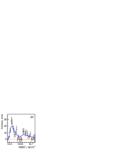
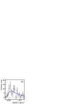
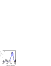
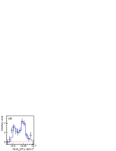
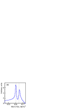
Figure 1: (a)–(d) Fitted line shapes of the $Z_{b}(10610)$ and $Z_{b}(10650)$ states in the $B^{(*)}\bar{B}^{*}$ and $\pi h_{b}(mP)$ ($m=1,2$) channels and (e) the predicted line shape in the $\pi\Upsilon(1S)$ channel [plots for $\pi\Upsilon(2S)$ and $\pi\Upsilon(3S)$ look similar and are not shown). Vertical lines indicate $B\bar{B}^{*}$ and $B^{*}\bar{B}^{*}$ thresholds. Fit results are given in Eq. (16].

As an application for our approach, we consider $1^{+-}$ $Z_{b}(10610)$ and $Z_{b}(10650)$ states residing near the $B\bar{B}^{*}$ and $B^{*}\bar{B}^{*}$ thresholds, respectively, that are produced in $\Upsilon(5S)$ decays $\Upsilon(5S)\to\pi Z_{b}$ and that are seen in seven decay channels: $Z_{b}\to B\bar{B}^{*}$, $B^{*}\bar{B}^{*}$, $\pi\Upsilon(nS)$ ($n=1,2,3$), and $\pi h_{b}(mP)$ ($m=1,2$) Belle:2011aa ; Adachi:2012cx . The quantum numbers of the final quarkonia fix the angular momenta of the inelastic final states in Eq. (12) to $l=0$ for all $\pi\Upsilon(nS)$ final states and to $l=1$ for the $\pi h_{b}(mP)$ final states.

The fact that the $b$-quark mass $m_{b}\gg\Lambda_{\rm QCD}$ allows us to use heavy-quark spin symmetry (HQSS) to reduce the number of parameters. If the wave functions of negative-parity heavy-light $B$ mesons are taken in the form (the charge conjugation is defined as ${\hat{C}}M=\bar{M}$) $B=0^{-}_{q\bar{b}}$, $\bar{B}=0^{-}_{b\bar{q}}$, $B^{*}=1^{-}_{q\bar{b}}$, and $\bar{B}^{*}=-1^{-}_{b\bar{q}}$, then the Fierz transformation yields the following $1^{+-}$ combinations:

$$|B\bar{B}^{*}\rangle_{1^{+-}}=-\frac{1}{\sqrt{2}}\Bigl{[}(1^{-}_{b\bar{b}}\otimes 0^{-}_{q\bar{q}})_{S=1}+(0^{-}_{b\bar{b}}\otimes 1^{-}_{q\bar{q}})_{S=1}\Bigr{]},$$

$$|B^{*}\bar{B}^{*}\rangle_{1^{+-}}=\frac{1}{\sqrt{2}}\Bigl{[}(1^{-}_{b\bar{b}}\otimes 0^{-}_{q\bar{q}})_{S=1}-(0^{-}_{b\bar{b}}\otimes 1^{-}_{q\bar{q}})_{S=1}\Bigr{]},$$

which imply that Bondar:2011ev ; Voloshin:2011qa

$$\frac{g_{[\pi\Upsilon(nS)][B^{*}\bar{B}^{*}]}}{g_{[\pi\Upsilon(nS)][B\bar{B}^{*}]}}=-1,\quad\frac{g_{[\pi h_{b}(mP)][B^{*}\bar{B}^{*}]}}{g_{[\pi h_{b}(mP)][B\bar{B}^{*}]}}=1,$$ (14)

where the total angular momentum of the light-quark contribution in the latter case is to be provided by one unit of angular momentum that is explicitly accounted for in Eq. (12). Once the elastic channels $B\bar{B}^{*}$ and $B^{*}\bar{B}^{*}$ are produced in the decays of the $\Upsilon(5S)$, the ratio of the sources $\xi$ is subject to the same heavy-quark constraint,

$$\xi=\frac{g_{[\pi\Upsilon(5S)][B^{*}\bar{B}^{*}]}}{g_{[\pi\Upsilon(5S)][B\bar{B}^{*}]}}=-1.$$ (15)

In the same limit, the direct interaction in the $B^{(*)}\bar{B}^{*}$ system can be parametrized in terms of only two parameters, $\gamma_{s}$ and $\gamma_{t}$, which are related to the contact potentials used in Nieves:2012tt as $\gamma_{s}^{-1}=(2\pi)^{2}\mu(C_{0a}+C_{0b})$ and $\gamma_{t}^{-1}=(2\pi)^{2}\mu(C_{0a}-3C_{0b})$ ($\mu_{1}\approx\mu_{2}\equiv\mu$). Then Hanhart:2011jz

$$t^{v}=\frac{1}{(2\pi)^{2}\mu}\frac{1}{\mbox{Det}}\left(\begin{array}[]{cc}\frac{1}{2}(\gamma_{s}+\gamma_{t})+ik_{2}&\frac{1}{2}(\gamma_{t}-\gamma_{s})\\ \frac{1}{2}(\gamma_{t}-\gamma_{s})&\frac{1}{2}(\gamma_{s}+\gamma_{t})+ik_{1}\end{array}\right),$$

with $\mbox{Det}=\gamma_{s}\gamma_{t}-k_{1}k_{2}+(i/2)(\gamma_{s}+\gamma_{t})(k_{1}+k_{2})$.

The bare pole is included in the formalism in order to provide more flexibility in the fitting process—in particular, it allows one to have two poles near the threshold even in the single-channel case. However, it should be omitted if its presence is not requested by the data. Thus, since we get a very good fit even without the bare pole, we refrain from its inclusion, thus setting $f_{\alpha}=\lambda_{i}=0$ and $M_{0}\to\infty$ in all formulas. As an experimental input we use

• background-subtracted and efficiency-corrected distributions in $M$ for the $B^{(*)}\bar{B}^{*}$ and $\pi h_{b}(nP)$ channels Adachi:2012cx ; Belle:2011aa with floating normalization in each channel;

• ratios of total branching fractions, $\mbox{Br}^{e}_{B\bar{B}^{*}}/\mbox{Br}^{e}_{B^{*}\bar{B}^{*}}$, $\mbox{Br}^{in}_{i}/\mbox{Br}^{e}_{B^{*}\bar{B}^{*}}$ Adachi:2012cx ; Belle:2011aa ; Adachi:2011ji ; Garmash:2014dhx , where index $i$ runs over all five inelastic channels $\pi\Upsilon(nS)$ and $\pi h_{b}(mP)$.

We do not use the information on the $Z_{b}^{(\prime)}$ line shapes in the $\pi\Upsilon(nS)$ channels, since in the one-dimensional fit it is not possible to correctly take into account the interference with the nonresonant continuum, which is significant in the $\Upsilon(5S)\to\pi^{+}\pi^{-}\Upsilon(nS)$ transitions. Inclusion of the $\pi\Upsilon(nS)$ line shapes would require a multidimensional analysis, which is beyond the scope of this Letter; however, it is straightforward from the theoretical point of view. In order to come to a converging fit we are, therefore, forced to impose that $g_{[\pi\Upsilon(nS)][B\bar{B}^{*}]}=-g_{[\pi\Upsilon(nS)][B^{*}\bar{B}^{*}]}$ for $n=1,2,3$, as given by Eq. (14). Meanwhile, we leave $g_{[\pi\Upsilon(5S)][B\bar{B}^{*}]}$ and $g_{[\pi\Upsilon(5S)][B^{*}\bar{B}^{*}]}$ as well as $g_{[\pi h_{b}(mP)][B\bar{B}^{*}]}$ and $g_{[\pi h_{b}(mP)][B^{*}\bar{B}^{*}]}$ unconstrained. The line shapes in the $\pi\Upsilon(nS)$ channels come out as our prediction. To take into account the experimental resolution, we convolve all the distributions with a Gaussian function with $\sigma=6$ MeV. Results of the simultaneous fit are shown in Figs. 1(a)–1(d). The developed parametrization provides a very good description of the experimental data, with a confidence level of 76%. Predicted line shapes in the $\pi\Upsilon(nS)$ channels look reasonably similar to the experimental data Garmash:2014dhx ; an example of such a distribution is shown in Fig. 1(e). It turns out that parameter $\kappa$, defined in Eq. (5), is practically unconstrained by the fit; thus, we fix it to 1 GeV. From the fit we find

$$\xi=\displaystyle\frac{g_{[\pi\Upsilon(5S)][B^{*}\bar{B}^{*}]}}{g_{[\pi\Upsilon(5S)][B\bar{B}^{*}]}}=-0.84\pm 0.05,$$

$$\displaystyle\frac{g_{[\pi h_{b}(1P)][B^{*}\bar{B}^{*}]}}{g_{[\pi h_{b}(1P)][B\bar{B}^{*}]}}=2.4\pm 0.6,$$ (16)

$$\displaystyle\frac{g_{[\pi h_{b}(2P)][B^{*}\bar{B}^{*}]}}{g_{[\pi h_{b}(2P)][B\bar{B}^{*}]}}=2.4\pm 0.7.$$

Deviations of these parameters from the predictions of HQSS—see Eqs. (14) and (15)—might be explained by the close proximity of the $t$ matrix poles to the thresholds, which can result in an enhancement of the small explicit symmetry violation caused by $\Lambda_{\rm QCD}/m_{b}\neq 0$ Cleven:2011gp . Another source of the deviation of $\xi$ from the prediction of the HQSS may stem from a $D$-wave $b\bar{b}$ component as well as from possible non-$b\bar{b}$ components of the $\Upsilon(5S)$ wave function (cf. the discussion in Guo:2014qra ). The importance of the HQSS-breaking contributions for the proper description of the $Z_{b}^{(\prime)}$ line shapes was also stressed in Mehen:2013mva . It should be noticed that preliminary Belle data on the $B\bar{B}^{*}$ and $B^{*}\bar{B}^{*}$ channels are used in the current analysis; fit results could change for the final experimental data. The inclusion of the information on the $\pi\Upsilon(nS)$ line shapes in a future multidimensional analysis will help to improve the accuracy of the determination of the model parameters and will allow for drawing more firm conclusions about the underlying physics of the spectacular near-threshold phenomena called $Z_{b}(10610)$ and $Z_{b}(10650)$.

IV Conclusions

In this Letter we proposed a practical parametrization for the line shapes of the near-threshold state(s). Since the approach is based on the LSE for the coupled-channel problem, unitarity and analyticity constraints for the $t$ matrix are fulfilled automatically. This guarantees that all imaginary parts are included in a self–consistent way. Since there are good reasons to neglect direct interactions within the inelastic channels, at least for the systems discussed here, the inelastic channels enter the expressions additively which; this makes it particularly easy to extend the inelastic basis. While additional effects such as finite widths of the constituents and the FSI with the spectator may also play a role and should be included on top of the interactions considered in this Letter; nevertheless, the gross features of the coupled-channel problem are captured by the presented model and the parametrization based on it is expected to be realistic. Finally, we demonstrate the power of the suggested parametrization by the fit to the line shapes for the bottomoniumlike states $Z_{b}(10610)$ and $Z_{b}(10650)$, for which we obtain a very good description.

- (1) S. K. Choi et al. (Belle Collaboration), Phys. Rev. Lett. 91, 262001 (2003).
- (2) T. Abe et al. (Belle-II Collaboration), arXiv:1011.0352.
- (3) A. G. Drutskoy, F.-K. Guo, F. J. Llanes-Estrada, A. V. Nefediev, and J. M. Torres-Rincon, Eur. Phys. J. A 49, 7 (2013).
- (4) D. M. Asner et al., Int. J. Mod. Phys. A 24, 499 (2009).
- (5) M. F. M. Lutz et al. (PANDA Collaboration), arXiv:0903.3905.
- (6) N. Brambilla et al., Eur. Phys. J. C 71, 1534 (2011).
- (7) N. Brambilla et al., Eur. Phys. J. C 74, 2981 (2014).
- (8) X. H. Liu, F.-K. Guo, and E. Epelbaum, Eur. Phys. J. C 73, 2284 (2013).
- (9) W. Detmold, S. Meinel, and Z. Shi, Phys. Rev. D 87, 094504 (2013).
- (10) I. V. Danilkin, V. D. Orlovsky, and Yu. A. Simonov, Phys. Rev. D 85, 034012 (2012).
- (11) I. V. Danilkin and Yu. A. Simonov, Phys. Rev. D 81, 074027 (2010).
- (12) K. Nakano, Phys. Rev. C 26, 1123 (1982).
- (13) C. Hanhart, Phys. Lett. B 715, 170 (2012).
- (14) V. Baru, C. Hanhart, Yu. S. Kalashnikova, A. E. Kudryavtsev, and A. V. Nefediev, Eur. Phys. J. A 44, 93 (2010).
- (15) C. Hanhart, Yu. S. Kalashnikova, and A. V. Nefediev, Eur. Phys. J. A 47, 101 (2011).
- (16) K. A. Olive et al. (Particle Data Group Collaboration), Chin. Phys. C 38, 090001 (2014).
- (17) A. Bondar et al. (Belle Collaboration), Phys. Rev. Lett. 108, 122001 (2012).
- (18) I. Adachi et al. (Belle Collaboration), arXiv:1209.6450.
- (19) A. E. Bondar, A. Garmash, A. I. Milstein, R. Mizuk, and M. B. Voloshin, Phys. Rev. D 84, 054010 (2011).
- (20) M. B. Voloshin, Phys. Rev. D 84, 031502 (2011).
- (21) J. Nieves and M. P. Valderrama, Phys. Rev. D 86, 056004 (2012).
- (22) I. Adachi et al. (Belle Collaboration), Phys. Rev. Lett. 108, 032001 (2012).
- (23) A. Garmash et al. (Belle Collaboration), Phys. Rev. D 91, 072003 (2015).
- (24) M. Cleven, F.-K. Guo, C. Hanhart, and U.-G. Meißner, Eur. Phys. J. A 47, 120 (2011).
- (25) F.-K. Guo, U.-G. Meißner, and C. P. Shen, Phys. Lett. B 738, 172 (2014).
- (26) T. Mehen and J. W. Powell, Phys. Rev. D 88, 034017 (2013).