Event-based and LHV simulation of an EPR-B experiment: epr-simple and epr-clocked

Richard D. Gill¹¹1Mathematical Institute, Leiden University, Netherlands
https://www.math.leidenuniv.nl/~gill
This is version 11 of this preprint. Earlier versions incorrectly stated
that documentation of Michel Fodje’s simulation was inexistent. This
version also contains some further explanations of my terminology.

(April 10, 2021)

Abstract

In this note, I analyse the data generated by M. Fodje’s (2013, 2014) simulation programs “epr-simple” and “epr-clocked”. They are written in Python and were published on Github. Inspection of the program descriptions shows that they make use of the detection-loophole and the coincidence-loophole respectively.

I evaluate them with appropriate modified Bell-CHSH type inequalities: the Larsson detection-loophole adjusted CHSH, and the Larsson-Gill coincidence-loophole adjusted CHSH. The experimental efficiencies turn out to be approximately $\eta=81\%$ (close to optimal) and $\gamma=55\%$ (far from optimal). The observed values of CHSH are, as they must be, within the appropriate adjusted bounds. Fodjes’ detection-loophole model turns out to be very, very close to Pearle’s famous 1970 model, so the efficiency is very close to optimal. The model also has the same defect as Pearle’s: the joint detection rates exhibit signalling.

Fodje’s coincidence-loophole model is actually an elegant modification of his detection-loophole model. However, this particular construction prevents attainment of the optimal efficiency. Keywords and phrases: Bell’s theorem; detection loophole; computer simulation; event-based simulation.

Introduction

Michel Fodje, in 2013–2014, wrote two event-based simulation programs of EPR-B experiments called “epr-simple” and “epr-clocked”. The programs are written in the Python programming language and are freely available at https://github.com/minkwe/epr-simple and https://github.com/minkwe/epr-clocked. Descriptions are given at https://github.com/minkwe/epr-simple/blob/master/README.md and https://github.com/minkwe/epr-clocked/blob/master/README.md.

One can recognise from the program descriptions that the two programs respectively use the detection loophole (Pearle, 1970) and the coincidence loophole (Pascazio, 1986; Larsson and Gill, 2004) to reproduce (to a good approximation) the singlet state correlation function and thereby to violate the CHSH inequality. See the appendix for further information on the models. I initially imagined that the author was perhaps inspired by event-based simulations, based on these loopholes, which at that time had recently been published by Hans de Raedt and his collaborators, and were being discussed in various internet fora. However, he had come up with the ideas behind these models, as well as the particular implementation of the general ideas, completely by himself. He never studied the literature on these loopholes, or even considered them as “loopholes”. He just tried, independently, and successfully, to create local realistic event-based simulation models which reproduced most features of past experiments. He was certainly provoked by some remarks of mine. On an internet forum I wrote, and he quoted these words,

It is impossible to write a local realist computer simulation of a clocked experiment with no “non-detections”, and which reliably reproduces the singlet correlations. (By reliably, I mean in the situation that the settings are not in your control but are delivered to you from outside; the number of runs is large; and that this computer program does this not just once in a blue moon, by luck, but most times it is run on different people’s computers.)

Unfortunately, I did not explain in the same internet posting exactly what I meant by the word “clocked”(the emphasis was mine). It would have been better if I had used the word “pulsed”. I was thinking of those experiments in which the time axis is split into a regular sequence of fixed time intervals often called time slots, and in each time slot and in each wing of the experiment only one setting is chosen, at random, at the start of the time slot; then arbitrary algorithms in each wing of the experiment generate one binary outcome from the data which is collected there, and call it the outcome … even if there is no detection event there at all. With regularly spaced time slots and pulsed lasars this arrangement is nowadays quite standard.

If there is no detection event at all in one time slot they should use a fixed outcome, or even toss a coin to make one. Physicists (experimental or theoretical) tend to howl with disapproval at this suggestion. But I was serious. In medical statistics, this is called using the “intention to treat” principle, and is a standard way to deal with non-compliance in double-blind randomised clinical trials.

Fodje wrote that his simulations do not use post-selection or use the detection loophole since all emitted particles are detected. He did not refer to Larsson and Gill (2004), and apparently did not know the literature well, hence did not have any idea what I meant by the word “clocked”, though I certainly explained what I meant many times on the internet fora which we both frequented. I meant that the experiment should be set up and analysed as a long regular sequence or run of $N$ trials, each trial corresponding to a pair of time slots, one in each wing of the experiment. Per trial, in a CHSH-Bell inequalities type experiment, two random binary settings go in and two binary outcomes come out. In other experiments, exploring the whole correlation function, the settings are angles, e.g., in whole numbers of degrees, chosen again and again, uniformly at random, in each wing of the experiment. The outcomes are again binary.

Fodje’s “readme” sections on Github include extensive explanation of how the models work, but do not refer to the now extensive literature on the two loopholes which Fodje effectively exploits.

I study the experimental efficiency of the two models in the CHSH setting. For the detection loophole, the efficiency $\eta$ is defined to be the minimum over all setting pairs and over all permutations of the two parties Alice and Bob, of the probability that Party 1 detects a particle given that Party 2 has detected a particle. For the coincidence loophole it is defined in a similar way: the efficiency $\gamma$ is defined to be the minimum over all setting pairs and over all permutations of the two parties Alice and Bob, of the probability that Party 1 has a detection which is paired to Party 2’s detection, given that Party 2 has detected a particle.

If either loophole is present in the experiment, then the CHSH inequality is not applicable, or to be more precise, the statement that local hidden variables cannot violate CHSH is not true. I refer the reader to the survey paper Larsson (2014); arXiv eprint http://arxiv.org/abs/1407.0363. One needs to make further (untestable) assumptions such as the “fair sampling” hypothesis in order to deduce impossibility of local hidden variables from violation of CHSH. However, it is not difficult to modify CHSH to take account of the possibly differential “post-selection”of particle pairs which is allowed by these two loopholes. The result is two bounds, replacing the usual bound “2”: $4/\eta-2$ for the detection loophole, and $6/\gamma-4$ for the coincidence loophole; see Larsson (2014) formula (38) and formulas (50), (51), (52). Note that when $\eta=1$ the detection loophole bound equals the usual CHSH bound 2, but as $\eta$ decreases from 1, the bound increases above 2, at some point passing the best quantum mechanical prediction $2\sqrt{2}$ (the Tsirelson bound) and later even achieving the absolute bound 4. The bound is sharp: one can come up with local hidden variable models which exactly achieve the bound at the given efficiency. In particular, with $\eta=2/3$ the detection loophole bound is 4, saying that it is possible for three of the four CHSH correlations to achieve their natural upper limit $+1$ and one of them its lower natural limit $-1$ .

The coincidence loophole bound is also attainable, and for the same value of the efficiency, worse. In particular, already with $\gamma=3/4$ one can attain three perfect correlations and one perfect anti-correlation.

epr-simple

The programme epr-simple uses the detection loophole (Pearle, 1970) so as to simulate violation of the CHSH inequality in a local-realistic way. The simulated experiment can be characterised as a pulsed experiment. At each of a long sequence of discrete time moments, two new particles are created at the source, and dispatched to two detectors. At the detectors, time and time again, a new pair of random settings is generated. The two particles are measured according to the settings and the outcome is either $+1$ , $-1$ , or $0$ ; the latter corresponding to “no detection”.

If either particle is not detected, the pair is rejected.

epr-simple only outputs some summary statistics for the accepted pairs. I added a few lines of code to the program so that it also outputs the “missing data”. Not being an expert in Python programming, my additional code is pretty simple.

First of all, I reduced the total number of iterations to 10 million. The original code has 50 million, and this lead to memory problems on the (virtual) Linux Mint system which I used for Python work. Secondly, I added a code line “numpy.random.seed(1234)”in the block of code called “class Simulation(object)”, so that identical results are obtained every time I run the code. This means that others should be able to reproduce the numerical results which I analyse here, exactly.

Finally, in the part of the code which outputs the simulation results for a test of the CHSH inequality, I added some lines to preserve the measurement outcomes in the case either measurement results in “zero” and then to cross-tabulate the results.

By the way, for his test of CHSH, Michel Fodje (thinking of the polarization measurements in quantum optics) took the angles 0 and 45 degrees for Alice’s settings, and 22.5 and 67.5 for Bob. I have changed these to 0 and 90 for Alice, and 45 and 135 for Bob, as is appropriate for a spin-half experiment.

for k,(i,j) in enumerate([(a,b),(a,bp), (ap,b), (ap, bp)]):

sel0 = (adeg==i) & (bdeg==j) # New variable

sel = (adeg==i) & (bdeg==j) &

(alice[:,1] != 0.0) & (bob[:,1] != 0.0)

Ai = alice[sel, 1]

Ai0 = alice[sel0, 1] # New variable

Bj = bob[sel, 1]

Bj0 = bob[sel0, 1] # New variable

print "%s: E(%5.1f,%5.1f), AB=%+0.2f, QM=%+0.2f" %

(DESIG[k], i, j, (Ai*Bj).mean(),

-numpy.cos(numpy.radians(j-i)))

npp = ((Ai0 == 1) & (Bj0 == 1)).sum() # New variable

np0 = ((Ai0 == 1) & (Bj0 == 0)).sum() # New variable

npm = ((Ai0 == 1) & (Bj0 == -1)).sum() # New variable

n0p = ((Ai0 == 0) & (Bj0 == 1)).sum() # New variable

n00 = ((Ai0 == 0) & (Bj0 == 0)).sum() # New variable

n0m = ((Ai0 == 0) & (Bj0 == -1)).sum() # New variable

nmp = ((Ai0 == -1) & (Bj0 == 1)).sum() # New variable

nm0 = ((Ai0 == -1) & (Bj0 == 0)).sum() # New variable

nmm = ((Ai0 == -1) & (Bj0 == -1)).sum() # New variable

print npp, np0, npm # Print out extra data

print n0p, n00, n0m # Print out extra data

print nmp, nm0, nmm # Print out extra data

CHSH.append( (Ai*Bj).mean())

QM.append( -numpy.cos(numpy.radians(j-i)) )

I ran epr-simple, redirecting the output to a text file called “data.txt”. In a text editor, I deleted all but 12 lines of that file – the lines containing the numbers which are read into R, and then printed out by the R code below. I omit the output tables of numbers here, to save space.

setwd("~/Desktop/Bell/Minkwe/minkwe_v7")

data <- as.matrix(read.table("data.txt"))

colnames(data) <- NULL

data[1:3, ]

data[4:6, ]

data[7:9, ]

data[10:12, ]

dim(data) <- c(3, 2, 2, 3)

Outcomes <- as.character(c(1, 0, -1))

Settings <- as.character(c(1, 2))

dims <- list(AliceOut = Outcomes, AliceIn = Settings,

BobIn = Settings, BobOut = Outcomes)

dimnames(data) <- dims

data <- aperm(data, c(1, 4, 2, 3))

data

rho <- function(D) (D[1, 1] + D[3, 3] - D[1, 3] - D[3, 1]) /

(D[1, 1] + D[3, 3] + D[1, 3] + D[3, 1])

corrs <- matrix(0, 2, 2)

for(i in 1:2) {for (j in 1:2) corrs[i, j] <- rho(data[ , , i, j])}

contrast <- c(-1, +1, -1, -1)

S <- sum(corrs * contrast)

corrs

S ## observed value of CHSH

2 * sqrt(2) ## QM prediction (Tsirelson bound)

We see a nice violation of CHSH; $S=2.798796$ . However, a large number of particle pairs have been rejected.

eta <- function(D) (D[1, 1] + D[1, 3] + D[3, 1] + D[3, 3])/sum(D[ , -2])

etap <- function(D) (D[1, 1] + D[1, 3] + D[3, 1] + D[3, 3])/sum(D[-2, ])

efficiency <- matrix(0, 2, 2)

for(i in 1:2) {for (j in 1:2) efficiency[i, j] <- eta(data[ , , i, j])}

efficiencyp <- matrix(0, 2, 2)

for(i in 1:2) {for (j in 1:2) efficiencyp[i, j] <- etap(data[ , , i, j])}

efficiency; efficiencyp

etamin <- min(efficiency, efficiencyp)

etamin

It turns out that the minimum over all setting pairs, and over the two permutations of the set of two parties {Alice, Bob}, of the probability that Party 1 has an outcome given Party 2 has an outcome, is $\eta\approx 81\%$ .

A “correct” bound to the post-selected CHSH quantity $S$ is not $2$ , but $4/\eta-2$ (Larsson, 2014).

S # CHSH

4 / etamin - 2 # bound

The corrected bound turns out to be about $2.9$ , just above the Tsirelson bound $2\sqrt{2}\approx 2.8$ . The simulation generates results just below the bound: at about $2.8$ . The observed value of $S$ , the quantum mechanical prediction $2\sqrt{2}$ and the adjusted CHSH bound are all quite close together: the simulation model is pretty close to optimal.

epr-clocked

The program epr-clocked uses the coincidence loophole (Pascazio, 1986). Michel Fodje calls this a “clocked experiment” where he means that time is continuous, the times of detection of particles are random and unpredictable. (I would have preferred to reserve the word “clocked” as synonym for “pulsed”). Because Alice and Bob’s particles have different, random, delays (influenced by the detector settings which they meet), one cannot identify which particles were originally part of which particle pairs. Moreover, a small number of particles did not get detected at all, compounding this problem.

The experimenter scans through the data looking for detections which are within some short time interval of one another. This is called the detection window. Unpaired detections are discarded.

I ran the program, setting the spin to equal 0.5, and an experiment of duration 10 seconds. I let Alice and Bob use the settings for a CHSH experiment: Alice uses angles 0 and 90 degrees, Bob uses angles 45 and 135 degrees. (As in epr-simple, Michel Fodje took the angles corresponding to a polarization experiment instead of a spin experiment). I set the numpy random seed to the values “1234”, “2345”, and “3456”prior to running the source program, Alice’s station program, and Bob’s station programme respectively. This should make my results exactly reproducible … but it doesn’t quite achieve that, because the 10 second duration of the experiment is ten seconds in “real time”. It therefore depends on queries by the program of the actual time in the real world outside the computer, and this process itself can take different lengths of time on each new run. However, the difference between the data obtained in different runs (with the same seed) should be negligeable: the total number of particle pairs will vary slightly, but their initial segments should coincide.

In order to get a strictly reproducible simulation, I rewrote one section of the program “source.py”. Below is my replacement code. Instead of running for 10 seconds of real time, the code simply generates exactly 200 000 emissions.

def run(self, duration=10.0):

N = 200000

n = 1

print "Generating spin-%0.1f particle pairs" % (self.n/2.0)

while n <= N:

self.emit()

n = n + 1

self.save(’SrcLeft.npy.gz’, numpy.array(self.left))

self.save(’SrcRight.npy.gz’, numpy.array(self.right))

print "%d particles in ’SrcLeft.npy.gz’" % (len(self.left))

print "%d particles in ’SrcRight.npy.gz’" % (len(self.right))

The standard output gave me the following information:

# No. of detected particles

# Alice: 199994

# Bob: 199993

# Calculation of expectation values

# Settings N_ab

# 0, 45 27416

# 0, 135 27512

# 90, 45 27345

# 90, 135 27425

# CHSH: <= 2.0, Sim: 2.790, QM: 2.828

Notice the total number of detected particles on either side, and the total numbers of coincidences for each of the four setting pairs. The total number of coincidence pairs is a bit more than 100 thousand; the total number of detections on either side is almost 200 thousand. We have a rather poor experimental efficiency of about 55%.

Npairs <- 27416 + 27512 + 27345 + 27425

Nsingles <- 199994

Npairs; Nsingles

gamma <- Npairs/Nsingles

gamma

6 / gamma - 4

The “correct” bound to the coincidence-selected CHSH quantity $S$ is not 2. In fact, we do not know it exactly, but a correct bound is conjectured to be $6/\gamma-4$ (Larsson, 2014). Here, $\gamma$ is the effective efficiency of the experiment measured as the chance that a detected particle on one side of the experiment will be accepted as part of a coincidence pair. Notice that at $\gamma=1$ (full efficiency) the adjusted bound is equal to the usual bound 2, but that as it decreases from 100% the bound rapidly increases. At $\gamma=3/4$ it reaches its natural maximum of 4.

At the observed efficiency of about 55%, the corrected CHSH bound in this experiment is close to 7, far above the natural and absolute bound 4.

Because the efficiency is lower than in epr-simple, while the proper bound (adjusted CHSH) is higher, this experiment is a good deal worse than the previous one in terms of efficiency. It wouldn’t be too difficult, at this level of experimental efficiency, to tune parameters of this model so as to get the observed value of CHSH up to its natural maximum of 4.

Incidentally, running epr-clocked many times, I experienced quite a few failures of the program “analyse.py”which is supposed to extract the coincidence pairs from the two data files. It seems that the Larsson algorithm for finding the pairs, which Fodje has adopted for this part of the data analysis, is failing in some circumstances. I could not find out what was the cause of this.

Fortunately it is now rather easy to import Numpy (“numerical python”) binary data files into R using the package “RcppCNPy”. It should also not be difficult to find a suitable alternative to Larsson’s matching algorithm in the computer science literature and probably freely available in C++ libraries. Algorithms written in C++ can often easily be made available in R via “Rcpp”. Hence one could replace Michel Fodje’s “analyse.py” by one’s own data analysis script; this would also allow a “proper”computation of the efficiency $\gamma$ , taking the minimum over the efficiencies for each setting pair and both permutations of the two parties Alice and Bob.

References

R.D. Gill (2015, 2020), Pearle’s Hidden-Variable Model Revisited. Entropy 2020, 22 (1), 1, https://doi.org/10.3390/e22010001; http://arxiv.org/abs/1505.04431

J.-A. Larsson (2014), Loopholes in Bell Inequality Tests of Local Realism, J. Phys. A 47 424003 (2014). http://arxiv.org/abs/1407.0363

S. Pascazio (1986), Time and Bell-type inequalities, Phys. Letters A 118, 47-53.

P.M. Pearle (1970), Hidden-Variable Example Based upon Data Rejection, Phys. Rev. D 2, 1418-1425.

Appendix

The appendices below contain mathematical formulas of the two simulation models. I have done my best to extract these faithfully from the original Python code and accompanying explanations by the author Michel Fodje. I have earlier published translations into the R language: http://rpubs.com/gill1109/epr-simple, http://rpubs.com/gill1109/epr-clocked-core, http://rpubs.com/gill1109/epr-clocked-full

Appendix: epr-simple

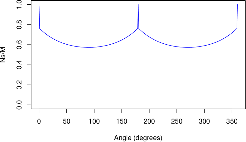
Here is a little simulation experiment with (my interpretation in R of) epr-simple. I plot the simulated correlation function and also the acceptance rate. With an effective sample size of $N\approx 0.8\times 10^{6}$ , the statistical error in simulated estimated correlation coefficients is roughly of size 0.001, well below the resolution of the graphs plotted below. Thus the small visible deviations from the theoretical negative cosine curve are for real. I simplify the model by taking spin = 1/2. Formulas are further simplified by a sign flip of all measurement outcomes, which by the symmetries of the model, does not change the observed data statistics.

set.seed(9875)

## For reproducibility. Replace integer seed by your own,

## or delete this line and let your computer dream up one for you

## (it will use system time + process ID).

## Measurement angles for setting ’a’:

## directions in the equatorial plane

angles <- seq(from = 0, to = 360, by = 1) * 2 * pi/360

K <- length(angles)

corrs <- numeric(K) ## Container for correlations

Ns <- numeric(K) ## Container for number of states

beta <- 0 * 2 * pi/360 ## Measurement direction ’b’ fixed,

## in equatorial plane

b <- c(cos(beta), sin(beta)) ## Measurement vector ’b’

M <- 10^6 ## Size of "pre-ensemble"

## Use the same, single sample of ’M’ realizations of hidden

## states for all measurement directions. This saves a lot of time,

## and reduces variance when we look at *differences*.

e <- runif(M, 0, 2*pi)

ep <- e + pi

U <- runif(M)

p <- (sin(U * pi / 2)^2)/2

## Loop through measurement vectors ’a’

## (except last = 360 degrees = first)

for (i in 1:(K - 1)) {

alpha <- angles[i]

ca <- cos(alpha - e)

cb <- cos(beta - ep)

A <- ifelse(abs(ca) > p, sign(ca), 0)

B <- ifelse(abs(cb) > p, sign(cb), 0)

AB <- A*B

good <- AB != 0

corrs[i] <- mean(AB[good])

Ns[i] <- sum(good)

}

corrs[K] <- corrs[1]

Ns[K] <- Ns[1]

plot(angles * 180/pi, corrs, type = "l", col = "blue",

xlab = "Angle (degrees)", ylab = "Correlation")

lines(angles * 180/pi, - cos(angles), col = "black")

legend(x = 0, y = 1.0, legend = c("epr-simple", "neg cosine"),

text.col = c("blue", "black"), lty = 1, col = c("blue", "black"))

plot(angles * 180/pi, Ns / M, type = "l", col = "blue",

xlab = "Angle (degrees)", ylim = c(0, 1))

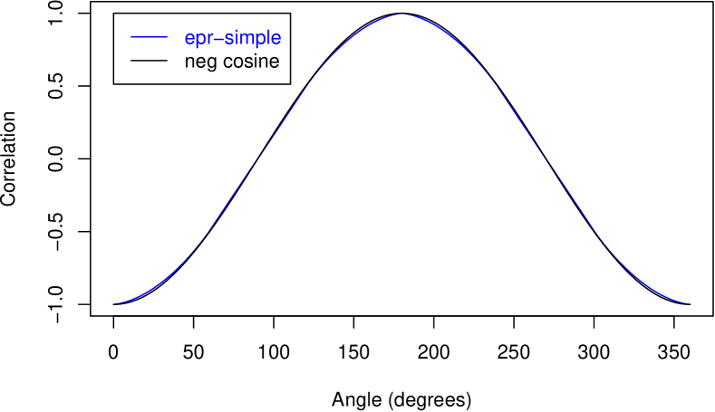
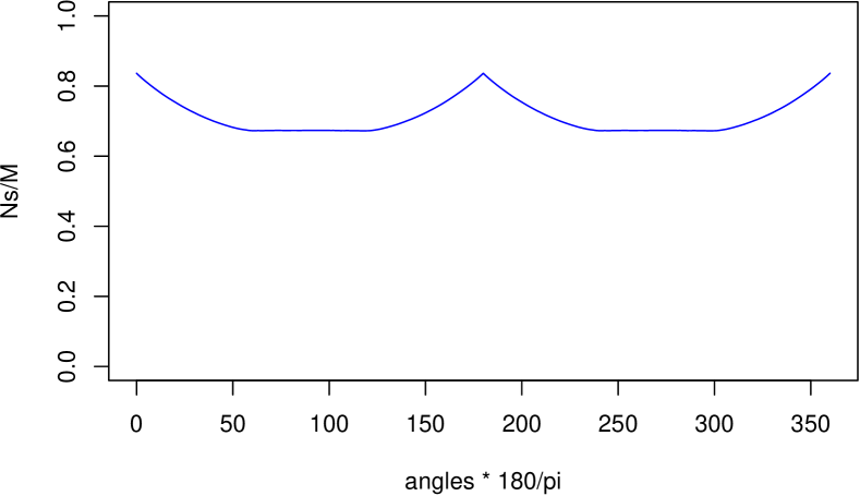
The detection loophole model used here is very simple. There is a hidden variable $E$ uniformly distributed in $[0,2\pi]$ . Independently thereof, there is a second hidden variable $P$ taking values in $[0,1/2]$ . Its distribution is determined by the relation $P=\sin^{2}((\pi/2)U)/2$ where $U$ is uniform on $[0,1]$ . Alice and Bob’s measurement outcomes are $\text{sign}\cos(E-\alpha)$ and $\text{sign}\cos(E-\beta+\pi)$ respectively, if each of their particles is detected. Alice’s particle is detected if and only if $\text{abs}(\cos(E-\alpha))>P$ and Bob’s if and only if $\text{abs}(\cos(E-\beta))>P$ .

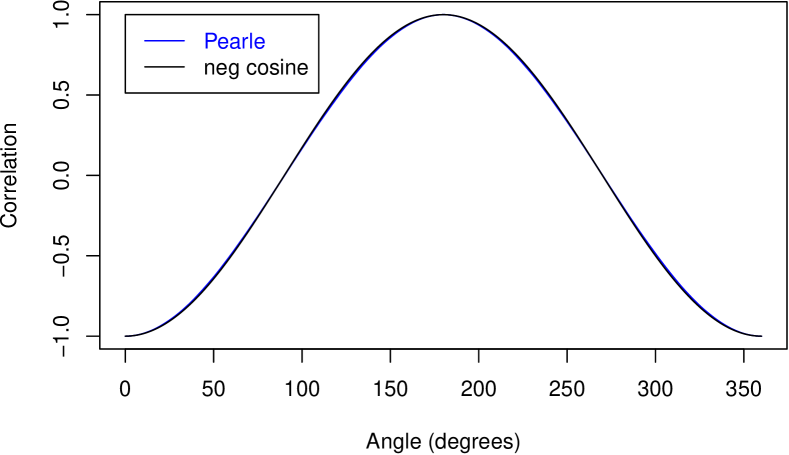
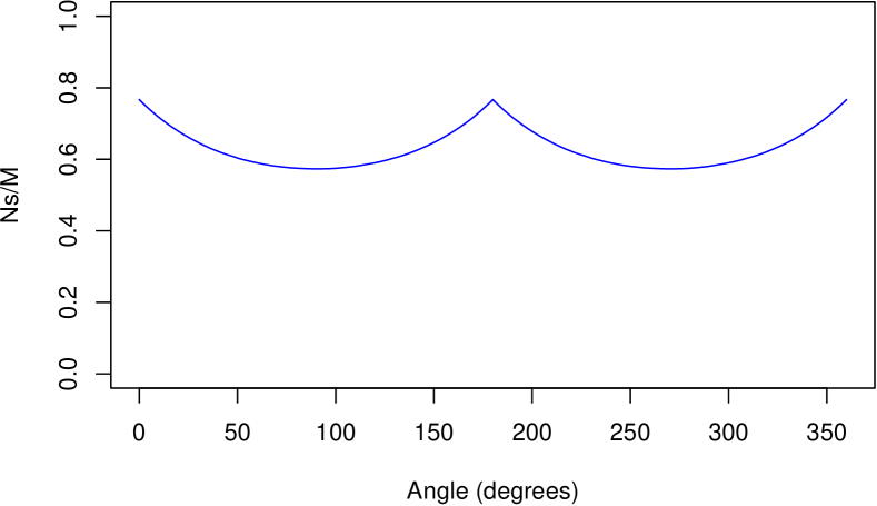
Pearle (1970) characterized mathematically the set of all probability distributions of $P$ which would give us the singlet correlations exactly (and for measurement directions in space, not just in the plane). He also picks out one particularly simple model in the class. His special choice has $P=(2/\sqrt{V})-1\in[0,1]$ where $V$ is uniform on $[1,4]$ , first expressed in this way by myself in 2014, see http://rpubs.com/gill1109/pearle and Gill (2015.)

Below, the simulation is modified accordingly: just one line of code is altered. Now the experimental and theoretical curves are indistinguishable.

# p <- (sin(U * pi / 2)^2)/2 ## epr-simple

p <- 2/sqrt(1 + 3 * U) - 1 ## Pearle (1970) model

## Loop through measurement vectors ’a’

## (except last = 360 degrees = first)

for (i in 1:(K - 1)) {

alpha <- angles[i]

ca <- cos(alpha - e)

cb <- cos(beta - ep)

A <- ifelse(abs(ca) > p, sign(ca), 0)

B <- ifelse(abs(cb) > p, sign(cb), 0)

AB <- A*B

good <- AB != 0

corrs[i] <- mean(AB[good])

Ns[i] <- sum(good)

}

corrs[K] <- corrs[1]

Ns[K] <- Ns[1]

plot(angles * 180/pi, corrs, type = "l", col = "blue",

xlab = "Angle (degrees)", ylab = "Correlation")

lines(angles * 180/pi, - cos(angles), col = "black")

legend(x = 0, y = 1.0, legend = c("Pearle", "neg cosine"),

text.col = c("blue", "black"), lty = 1, col = c("blue", "black"))

plot(angles * 180/pi, Ns / M, type = "l", col = "blue",

xlab = "Angle (degrees)",

main = "Rate of detected particle pairs", ylim = c(0, 1))

Appendix: epr-clocked

Here is the core part of (my interpretation in R of) epr-clocked: the emission of a pair of particles, supposing that both are detected and identified as belonging to a pair. However, if the detection times of the two particles are too far apart (larger than the so-called coincidence window), the pair is rejected. This would correspond to running the full epr-clocked model with very low emission rate. I have simplified the model by fixing spin = 1/2. To save computer time and memory, I re-use the hidden variables $E$ (“e”) and $U$ from epr-simple.

Again, I plot the simulated correlation function and also the acceptance rate.

coincWindow <- 0.0004

ts <- pi * 0.03 ## timescale

asym <- 0.98 ## asymmetry parameter

p <- 0.5 * sin(U * pi / 6)^2

ml <- runif(M, asym, 1) ## small random jitter, left

mr <- runif(M, asym, 1) ## small random jitter, right

## Loop through measurement vectors ’a’

## (except last = 360 degrees = first)

for (i in 1:(K - 1)) {

alpha <- angles[i]

Cl <- (0.5/pi) * cos(e - alpha) ## cos(e-a), left

Cr <- (0.5/pi) * cos(ep - beta) ## cos(e-a), right

tdl <- ts * pmax(ml * p - abs(Cl), 0) ## time delays, left

tdr <- ts * pmax(mr * p - abs(Cr), 0) ## time delays, right

A <- sign(Cl) ## measurement outcomes, left

B <- sign(Cr) ## measurement outcomes, right

AB <- A * B ## product of outcomes

good <- abs(tdl-tdr) < coincWindow

corrs[i] <- mean(AB[good])

Ns[i] <- sum(good)

}

corrs[K] <- corrs[1]

Ns[K] <- Ns[1]

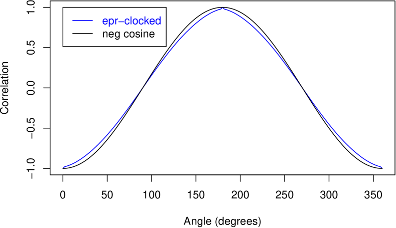
plot(angles * 180/pi, corrs, type = "l", col = "blue",

main = "epr-clocked",

xlab = "Angle (degrees)", ylab = "Correlation")

lines(angles * 180/pi, - cos(angles), col = "black")

legend(x = 0, y = 1.0, legend = c("epr-clocked", "neg cosine"),

text.col = c("blue", "black"), lty = 1, col = c("blue", "black"))

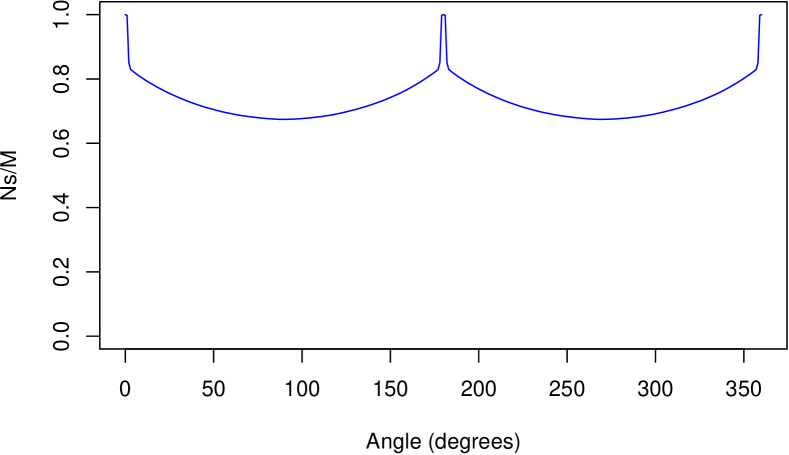
plot(angles * 180/pi, Ns / M, type = "l", col = "blue",

xlab = "Angle (degrees)",

main = "Rate of accepted particle pairs", ylim = c(0, 1))

I now remove the “small random jitter”, effectively setting the “asymmetry parameter” to 1. I rescale time so that the model is finally described in terms of a couple of standard probability distributions and two arbitrary constants.

coincWindow <- 0.034

p <- 8 * p ## Now p lies in the interval [0, 1]

## Loop through measurement vectors ’a’

## (except last = 360 degrees = first)

for (i in 1:(K - 1)) {

alpha <- angles[i]

Cl <- cos(e - alpha) ## cos(e-a), left

Cr <- - cos(e - beta) ## - cos(e-b), right

tdl <- pmax(p - 1.28 * abs(Cl), 0) ## time delays, left

tdr <- pmax(p - 1.28 * abs(Cr), 0) ## time delays, right

A <- sign(Cl) ## measurement outcomes, left

B <- sign(Cr) ## measurement outcomes, right

AB <- A * B ## product of outcomes

good <- abs(tdl-tdr) < coincWindow

corrs[i] <- mean(AB[good])

Ns[i] <- sum(good)

}

corrs[K] <- corrs[1]

Ns[K] <- Ns[1]

plot(angles * 180/pi, corrs, type = "l", col = "blue",

main = "epr-clocked",

xlab = "Angle (degrees)", ylab = "Correlation")

lines(angles * 180/pi, - cos(angles), col = "black")

legend(x = 0, y = 1.0, legend = c("epr-clocked", "neg cosine"),

text.col = c("blue", "black"), lty = 1, col = c("blue", "black"))

plot(angles * 180/pi, Ns / M, type = "l", col = "blue",

xlab = "Angle (degrees)",

main = "Rate of accepted particle pairs", ylim = c(0, 1))

The results are almost identical. The model is rather simple. There are just two hidden variables: a uniformly distributed angle $E$ in $[0,2\pi]$ and independently thereof, a random number $P=4\sin^{2}(\Theta)$ in $[0,1]$ where $\Theta$ is uniformly distributed in $[0,\pi/6]$ .

At Alice’s measurement device, where the setting is $\alpha$ , the measurement outcome is $\text{sign}\cos(E-\alpha)$ . At Bob’s measurement device, where the setting is $\beta$ , the measurement outcome is $\text{sign}\cos(E-\beta+\pi)$ .

During measurement, the particles experience time delays. Alice’s particle’s time delay is $\max(P-1.28|\cos(E-\alpha)|,0)$ and Bob’s is $\max(P-1.28|\cos(E-\beta)|,0)$ . Notice that if $\alpha=\beta$ or if $\alpha=\beta+\pi$ , the time delays of the two particles are identically equal to one another.

Finally, the two detections are accepted as belonging to one particle pair if the difference between their two delay times is less than 0.034; i.e., if they are detected within the same time interval of length maximally 0.034.

The full “epr-clocked” model adds on top of this simple core, some further (relatively small) sources of noise, which do serve to smooth out the anomalous spike when the two particles are measured in the same direction. Moreover, in his simulations, Michel Fodje does not measure at fixed directions, but samples measurement directions uniformly at random in the circle. When he computes correlations, he has to bin measurement directions, resulting in another source of noise, again further smoothing out anomalous features in the observed correlation curve.

Appendix: epr-clocked optimized

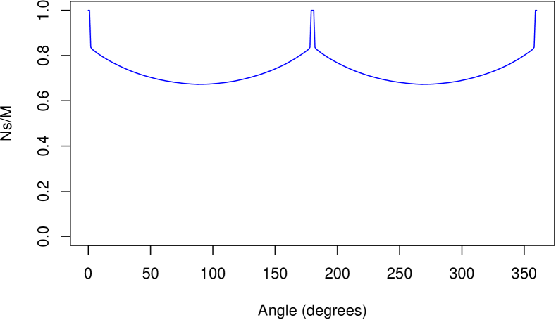
Inspection of the data-sets generated by the last model turned up something very interesting: the coincidence window is so small, that for most measurement settings, a pair of detections is only accepted as a pair if both particles experience the same, zero, time delay. But this means that the two detections are accepted as a pair if and only if $P<1.28|\cos(E-\alpha)$ and $P<1.28|\cos(E-\beta)|$ , because only in this case are both time delays identically equal to zero.

Now we are free to divide throughout in these inequalities by the constant 1.28 and absorb it into the random variable $P$ , and we are free to pick a different distribution for $P$ . So let us take $P$ the same as in the Pearle model. Let us also reduce the size of the coincidence window to make it almost impossible for particles which experience non-zero time delays to become paired with their partners.

coincWindow <- 0.000001

p <- 2/sqrt(1 + 3 * U) - 1 ## Pearle’s choice

## Loop through measurement vectors ’a’

## (except last = 360 degrees = first)

for (i in 1:(K - 1)) {

alpha <- angles[i]

Cl <- cos(e - alpha) ## cos(e-a), left

Cr <- - cos(e - beta) ## - cos(e-b), right

tdl <- pmax(p - abs(Cl), 0) ## time delays, left

tdr <- pmax(p - abs(Cr), 0) ## time delays, right

A <- sign(Cl) ## measurement outcomes, left

B <- sign(Cr) ## measurement outcomes, right

AB <- A * B ## product of outcomes

good <- abs(tdl-tdr) < coincWindow

corrs[i] <- mean(AB[good])

Ns[i] <- sum(good)

}

corrs[K] <- corrs[1]

Ns[K] <- Ns[1]

plot(angles * 180/pi, corrs, type = "l", col = "blue",

main = "epr-clocked optimized",

xlab = "Angle (degrees)", ylab = "Correlation")

lines(angles * 180/pi, - cos(angles), col = "black")

legend(x = 0, y = 1.0, legend = c("epr-clock-opt", "neg cosine"),

text.col = c("blue", "black"), lty = 1, col = c("blue", "black"))

plot(angles * 180/pi, Ns / M, type = "l", col = "blue",

xlab = "Angle (degrees)",

main = "Rate of accepted particle pairs", ylim = c(0, 1))

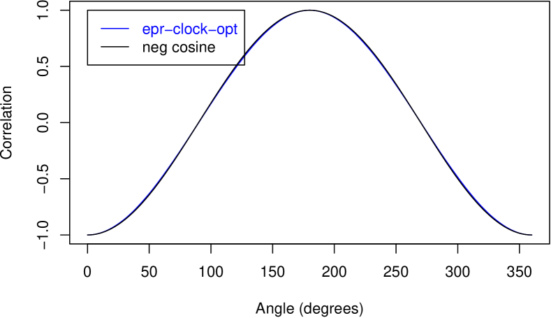
Conclusion: epr-clocked is actually a disguised and perturbed version of the detection loophole model epr-simple. It can therefore be slightly improved, just as epr-simple can be slightly improved. However, this will not help it achieve the maximum efficiency possible for coincidence-loophole models.