Symmetry Restored in Dibosons at the LHC?
Abstract
A number of LHC resonance search channels display an excess in the invariant mass region of 1.8 – 2.0 TeV. Among them is a excess in the fully hadronic decay of a pair of Standard Model electroweak gauge bosons, in addition to potential signals in the and dijet final states. We perform a model-independent cross-section fit to the results of all ATLAS and CMS searches sensitive to these final states. We then interpret these results in the context of the Left-Right Symmetric Model, based on the extended gauge group , and show that a heavy right-handed gauge boson can naturally explain the current measurements with just a single coupling . In addition, we discuss a possible connection to dark matter.
I Introduction
A number of searches for narrow resonances at the LHC now display peaks in the region of 1.8 – 2.0 TeV. Most prominently, a recent ATLAS search [1] for a resonance that decays to a pair of standard model (SM) gauge bosons contains a local excess of 3.4 (2.5 global) in the final state at approximately 2 TeV. Since the search is fully hadronic, there is only a limited ability to accurately distinguish gauge bosons, and consequently many of the events can also be interpreted as a or resonance, leading to excesses of 2.9 and 2.6 in these channels respectively.
Interest is further piqued when one analyses other resonance searches in a similar mass range. At approximately 1.8 TeV, both CMS [2] and ATLAS [3] observe excesses in the dijet distributions with a significance of 2.2 and 1 , respectively. In addition, a CMS search for resonant production [4] shows a 2.1 excess, and another CMS search [5] for a pair of vector bosons, but this time with a leptonically tagged , finds a 1.5 excess, both at approximately 1.8 TeV. With the exception of the three ATLAS selections in gauge boson pair production, all these possible signals are completely independent.
We analyze these excesses and perform a general cross-section fit to the data. It is of course important to not only look at possible signals in the distributions, and for that reason we include all relevant searches that may be sensitive to the same final states as those showing anomalies. These include diboson analyses from both ATLAS [6, 7, 8] and CMS [9, 10, 11]. In addition, many models that explain an excess of events in the dijet distribution with a charged mediator will also lead to a peak in a resonance search. Consequently, we also include the most sensitive searches for this particular final state from both ATLAS [12, 13] and CMS [14] in our study.
Combining all searches, we provide best fit signal cross sections for each of the final states analyzed in order to guide the model building process. In particular we find that the vector boson pair production searches are best described by a or final state, while is disfavoured via limits from semi-leptonic searches. In the associated Higgs production fit, we find preference for the final state, since an excess here is only seen in the single-lepton analysis. Finally, there is good agreement for a dijet signal between ATLAS and CMS, but nothing has been observed so far in the final state.
In order to explain these excesses we focus on the so-called Left-Right Symmetric Model (LRM) [15, 16, 17, 18, 19]. The LRM is based on the low-energy gauge group that can arise for example from an or GUT [20, 21]. Since there is a new gauge group in addition to the SM, the spectrum now contains both a and charged bosons. In general the model predicts , which is why we explain the various signals via resonant production and decay. By extending our cross-section fit to the LRM parameters, we find a region that can explain the excesses while avoiding all current exclusion bounds. We then examine where our fit suggests the mass of the should be and the discovery potential of the LHC for this state.
In a next step we also analyze the question of how such a model may be able to simultaneously explain dark matter (DM). If the is to mediate DM annihilation in the early universe the simplest scenario we can find is to include a new charged and neutral particle that would be relatively close in mass in order to co-annihilate effectively. Alternatively, we offer the concrete example that DM annihilation is mediated through the and the dark matter candidate is the neutral component of a new fermionic doublet. In this case, we see that resonant annihilation is required for the correct relic density and thus we predict the DM mass is .
II Experimental measurements and cross-section fits
In this section we give an overview over the ATLAS and CMS searches in which resonances in the mass range 1.8 – 2.0 TeV have been observed, or which provide constraints in the same or closely related final states. It is important to note that due to resolution, jet energy scale uncertainties and the limited number of events currently present in the excesses, peaks at 1.8 – 2.0 TeV can easily be compatible. Even though the most significant excess is observed in the ATLAS diboson search [1] at an invariant mass of 2.0 TeV, the majority of excesses are reported closer to an invariant mass of approximately 1.8 TeV. This is why we assume a resonance in the vicinity of 1.8 – 1.9 TeV in this analysis.
We analyze the results of these searches by performing cross-section fits in each channel individually. For this, we sum bins around this mass region according to the experimental width and jet energy scale of the particular study. We then perform a cut-and-count analysis on the event numbers in these enlarged signal regions. As input information we take into account the number of observed events, expected backgrounds, efficiencies, and systematic uncertainties, as published by ATLAS and CMS. Where necessary information is missing from the publications, we use estimations to the best of our knowledge. In App. A we list the data we use in more detail.
For the actual fit, we follow a frequentist approach. In the absence of systematic uncertainties, the number of events observed in the signal region, , follows a Poisson distribution
| (1) |
Here is the number of expected events, including the number of expected background events , and the product of the signal production cross section , branching ratios , integrated luminosity , and efficiency as well as acceptance factors . The systematic uncertainties on the background prediction and on the signal efficiency are approximated by Gaussian distributions. These nuisance parameters are marginalized. We neglect correlations between the different systematic uncertainties.
We then calculate a value for each signal cross section in each different final state, using at least pseudo-experiments. This gives us the significance of the deviation from the SM, best fit points, and confidence regions at and CL. We also calculate upper limits in a modified frequentist approach (CLs method [22]). In some of the signal regions, our simple cut-and-count strategy leads to model limits that are stronger than those presented by the experiments. In this case, the systematical background error and the signal efficiencies were rescaled to find agreement. Since many of our input parameters involve rough estimations, we have checked that the final results are stable under the variation of these input values.
In a next step, we perform combined fits to all studies that contribute to a particular final state. For the combination of individual values we use Fisher’s method. Again, we present the results in terms of values, best fit points, and confidence regions at and CL.
II.1 Vector boson pair production
| resonance analyses | ||||
|---|---|---|---|---|
| Analysis | Expected | Observed | Excess | Fitted cross |
| 95% CLs [fb] | 95% CLs [fb] | significance [] | section [fb] | |
| ATLAS hadronic [1] | 11.1 | 19.6 | 1.2 | 5.2 |
| CMS hadronic [9] | 12.2 | 17.9 | 1.0 | 6.0 |
| ATLAS single lepton [6] | 6.4 | 5.9 | 0.0 | 0.0 |
| CMS single lepton [5] | 7.2 | 8.1 | 0.3 | 1.2 |
| resonance analyses | ||||
|---|---|---|---|---|
| Analysis | Expected | Observed | Excess | Fitted cross |
| 95% CLs [fb] | 95% CLs [fb] | significance [] | section [fb] | |
| ATLAS hadronic [1] | 14.2 | 25.8 | 1.3 | 6.9 |
| CMS hadronic [9] | 11.9 | 17.5 | 1.0 | 5.8 |
| ATLAS single lepton [6] | 13.2 | 12.4 | 0.0 | 0.0 |
| CMS single lepton [5] | 14.9 | 16.8 | 0.3 | 2.4 |
| ATLAS double lepton [7] | 13.8 | 20.5 | 0.3 | 2.9 |
| CMS double lepton [5] | 14.4 | 27.4 | 1.5 | 10.0 |
| resonance analyses | ||||
|---|---|---|---|---|
| Analysis | Expected | Observed | Excess | Fitted cross |
| 95% CLs [fb] | 95% CLs [fb] | significance [] | section [fb] | |
| ATLAS hadronic [1] | 9.7 | 25.2 | 2.4 | 8.1 |
| CMS hadronic [9] | 11.7 | 17.1 | 1.0 | 5.7 |
| ATLAS double lepton [7] | 6.7 | 10.0 | 0.3 | 1.4 |
| CMS double lepton [5] | 7.0 | 13.4 | 1.5 | 4.9 |
The relevant searches targeting the resonant production of a pair of vector bosons either require both bosons to decay hadronically [1, 5] or one boson leptonically [6, 7, 5]. Unfortunately, branching ratio suppression dictates that searches where both bosons decay leptonically are currently uncompetitive.
In this set of analyses, the ATLAS fully hadronic search presently contains the largest single excess with reported by the experiment for an invariant mass of 2.0 TeV. Our cut-and-count analysis focuses on a slightly lower invariant mass window, leading to a reduced peak significance of , see Tab. 3. In order to fit the different final states we make use of the fact that the analysis has a mild discrimination between and bosons based on the invariant mass of a reconstructed ‘fat jet’. This leads to a slight preference for either a or final state to explain the excess present with a cross section of – 8 fb, see Tab. 2 and 3. Since a smaller peak is seen in the purely channel, a smaller cross section of fb is found for this channel, see Tab. 1. We again note that many of the events seen in the excess region are shared between all three final states; thus the total cross section in the excess region is substantially smaller than if we simply sum the three fitted cross sections together.
The CMS fully hadronic analysis search is very similar and also finds an excess in the same mass range, although with a slightly smaller signal of , see Tab. 1 – 3. In this analysis no real preference is seen for any of the different final states and a cross section of fb fits all three equally well.
More discrimination of the final states is available by using the semi-leptonic searches. Here, the one-lepton analyses require that a boson is present while the two-lepton searches reconstruct at least one boson. If we first examine the one-lepton searches we see that no excess is seen by ATLAS [6], while CMS [5] only has a very mild excess of . These searches place a significant constraint on the final state with ATLAS and CMS giving limits around 6 – 8 fb at 95% CLs. Removing one for the final state relaxes this limit to 12 fb, see Tab. 2.
In the two-lepton case, CMS [5] sees an excess of 1.5 which leads to a fitted cross section of 10 fb if we assume a pure final state, see Tab. 2, or 5 fb for a pure final state, see Tab. 3. The ATLAS search has similar sensitivity [7] but only observes a very small excess of .
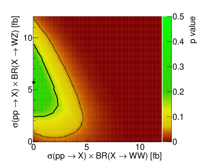
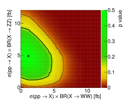
In Fig. 1 and Fig. 2 (left panel) we show the combined cross-section fit to all channels. Fig. 1 shows that both and final states fit the data well with a cross section of fb. However, we also see that a pure signal is disfavoured and could only describe the data in combination with another signal. The reason that the explanation is disfavoured is two-fold. First, the ATLAS and CMS single lepton analyses set an upper limit around fb at 95% CLs, but a cross section of this magnitude is required to fit the hadronic excesses. In addition, the CMS dilepton search [5] has a small excess that this channel cannot explain.
Finally the left panel of Fig. 2 shows that an equally good fit is possible with contributions from both a and final state, i. e. requiring both a charged and neutral resonance with similar mass. In combination, the standard model is disfavoured by when all vector boson pair production channels are included.
II.2 Associated vector-Higgs production
| resonance analyses | ||||
|---|---|---|---|---|
| Analysis | Expected | Observed | Excess | Fitted cross |
| 95% CLs [fb] | 95% CLs [fb] | significance [] | section [fb] | |
| ATLAS [8] | 33.0 | 30.0 | 0.0 | 0.0 |
| CMS [4] | 18.6 | 44.4 | 1.9 | 15.8 |
| CMS + hadronic vector [10] | 36.1 | 36.1 | 0.0 | 0.0 |
| CMS hadronic Higgs [11] | 12.5 | 13.2 | 0.1 | 1.0 |
| resonance analyses | ||||
|---|---|---|---|---|
| Analysis | Expected | Observed | Excess | Fitted cross |
| 95% CLs [fb] | 95% CLs [fb] | Significance [] | section [fb] | |
| ATLAS [8] | 15.0 | 14.0 | 0.0 | 0.0 |
| CMS + hadronic vector [10] | 31.8 | 31.8 | 0.0 | 0.1 |
| CMS hadronic Higgs [11] | 12.2 | 12.9 | 0.1 | 1.0 |
The experimental searches for a resonance that decays into a final state are varied. ATLAS looks for a Higgs that produces a pair with the or probed leptonically , or [8]. CMS has a similar search for but only examines the leptonic channel [4]. To probe vector bosons more generally, CMS has a fully hadronic search [11], but this has a limited ability to discriminate between and . Finally there is a CMS search for , again with a hadronic reconstruction of the vector boson [10].
Out of these searches, only the CMS study with a leptonic displays an significant excess with at 1.8 – 1.9 TeV. Interpreting this as a resonance that decays to leads to a fitted cross section of 16 fb, see Tab. 4. However, the fully hadronic CMS search is slightly in tension with this result as it reports a limit of 13 fb on the same final state. In the analyses that are sensitive to production, no significant excesses are seen, see Tab. 5. For this final state, the ATLAS semi-leptonic [8] and CMS fully hadronic [11] searches have similar sensitivities and set a 95% CLs limit of 14 fb and 13 fb respectively.
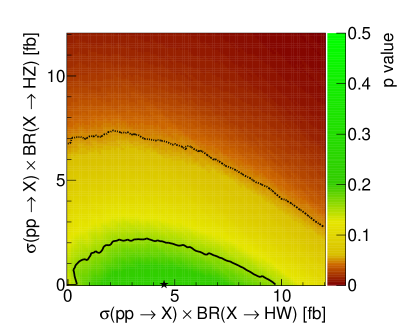
Combining all these searches into a single fit, we plot the preferred cross sections for and productions in the right panel of Fig. 2. We find that the best fit point has a cross section for production of fb, but is also compatible with the SM background at . Since the only excess is seen in a channel compatible with a in the final state, there is no evidence in the data for a signal in the channel.
II.3 Dijet production
Both the dijet search by ATLAS [3] and that by CMS [2] see an excess in the invariant mass distribution around 1.8 TeV. In our analysis, we find the excess in CMS is slightly more significant at 1.9 compared to 1.5 in ATLAS. However, since the CMS analysis is slightly more sensitive to a signal, the fitted cross section is actually smaller at fb, compared to ATLAS with 100 fb, see Tab. 6. In any case, the two signals seen by both experiments are remarkably similar and the combined best-fit signal cross section of fb can be seen in Fig. 7.
| Dijet resonance analyses | ||||
| Analysis | Expected | Observed | Excess | Fitted cross |
| 95% CLs [fb] | 95% CLs [fb] | Significance [] | section [fb] | |
| ATLAS dijet [3] | 131 | 217 | 1.5 | 101 |
| CMS dijet [2] | 92 | 173 | 1.9 | 90 |
II.4 Associated top-bottom production
| resonance analyses | ||||
| Analysis | Expected | Observed | Excess | Fitted cross |
| 95% CLs [fb] | 95% CLs [fb] | Significance [] | section [fb] | |
| ATLAS hadronic [12] | 155 | 203 | 0.6 | 31 |
| ATLAS leptonic [13] | 138 | 101 | 0.0 | 0 |
| CMS leptonic [14] | 76 | 67 | 0.0 | 0 |
The final analyses that we consider are the studies that look for the resonant production of a final state, see Tab. 7. ATLAS has two searches that focus on this signature, one that looks for the hadronic decay of the [12] and another that considers the leptonic channel [13]. On the CMS side, only one study exists, concentrating on the leptonic decay [14]. At the current time, only the ATLAS hadronic search contains a small excess in the region of 1.8 TeV. However, since this search was expected to have the poorest sensitivity, it is likely that this is purely a statistical fluctuation.
The strongest bound comes from the CMS leptonic search with an upper limit on the cross section of 70 fb at 95% CLs. However, we should also pay particular attention to the ATLAS leptonic search since this heavily influences our final model fits and interpretations. The reason is that at 1.8 TeV, the search records a signal 1.8 smaller than expected. We hesitate to call this an ‘underfluctuation’ because the search systematically measures a cross section 2 less than the background prediction across the whole mass probed (500 – 3000 GeV). Due to the construction of the CLs limit setting procedure, which weights the likelihood according to the agreement of the signal with the background, the systematically high background prediction does not result in a hugely significant shift in the 95% CLs limit (expected limit: 138 fb, observed limit: 101 fb).
However, in our cross-section fit, the search has a far greater effect on the overall value, since any additional signal predicted in this channel will be heavily penalized. For this reason, we perform two fits to the final state, one which includes the ATLAS leptonic search, shown in the left panel of Fig. 3, and one without, see the right panel of Fig. 3. In both plots we see that the best fit point is found without a signal present. However, including the leptonic ATLAS search results in a 1 allowed cross section of fb but removing the search allows this to increase to fb in combination with the dijet result.
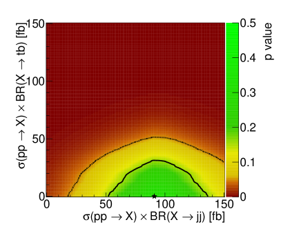
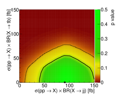
II.5 Channel comparison
| Fitted cross sections | ||
|---|---|---|
| Process | Fitted cross | Upper bound |
| section [fb] | (90% CL) | |
| 11.8 | ||
| 11.3 | ||
| 15.5 | ||
| 170 | ||
| 38 | ||
| (without ATLAS [13]) | 60 | |
By comparing the various fitted cross sections we can try to provide guidance on the kind of model required to fit the current data. We also note that this is not completely speculative since a combined analysis of the above searches finds that the standard model has a 2.9 discrepancy with the data due to various excesses present.
We first note that the required cross sections to correctly fit the data are very similar for and (which can be considered as roughly the same measurement) and , see Tab. 8. In our opinion this seriously motivates a model in which the resonant production particle carries charge, since the same particle can then be responsible for both final states. In addition, the fact that suggests to us that a model that predicts an equal branching ratio to these two modes should be considered.
In comparison, the dijet cross section for the signal is over an order of magnitude larger. In terms of finding a model to fit these excesses this is convenient, since the easiest way to produce such a high mass resonance will be through a quark coupling of appropriate strength. The same coupling will then automatically lead to a decay into a dijet final state.
Combining the , , and dijet final states thus naturally leads to a model with a charged resonance. Working with the principle of simplicity, we may expect the couplings of this resonance to be flavor diagonal and therefore predict that . Unfortunately there is no evidence for a signal in the final state and the 1 preferred region only extends to fb, which is roughly . However, we refer the reader to the discussion in Sec. II.4 where we note that the ATLAS leptonic search finds a cross section that is systematically 2 below the background prediction. Consequently, the fit is heavily influenced by this single result and we believe that it is also wise to study the cross section measurement when this analysis is removed. In this case, the 1 preferred region extends up to fb and is therefore perfectly compatible with the observed dijet signal.
III Interpretation in the Left-Right Symmetric Model
We now turn towards a specific model and interpret the observed excesses in the Left-Right Symmetric Model [19]. In Sec. III.1 we summarize the structure and key phenomenological properties of this framework. We then compare its predictions to the experimental data and perform a model parameter fit in Sec. III.2. Finally we discuss the prospect of observing signatures for this model during the upcoming LHC Run II in Sec. III.3.
III.1 Model essentials
In the Left-Right Symmetric Model (LRM) framework [19], the SM electroweak gauge group is extended to with the usual left-handed (right-handed) fermions of the SM transforming as doublets under . For instance, the left-handed (LH) quarks transform as , whereas the right-handed (RH) quarks transform as (1,2,1/3). The corresponding gauge couplings are denoted by , which are not in general equal, as well as . As a consequence of this symmetry, a RH neutrino must necessarily be introduced for each generation; neutrinos are thus naturally massive in this framework.
The SM is recovered by the breaking , where additional Higgs fields are required to break this symmetry generating the masses of the new gauge fields , . This breaking relates the and couplings to the usual SM hypercharge coupling . Note that since and are both well-measured quantities, only the ratio remains as a free parameter in the model. The new Higgs fields responsible for breaking are usually assumed to transform either as a doublet, , or as a triplet, , under the gauge group, and the neutral component obtains a multi-TeV scale vev, . The corresponding LH doublet or triplet Higgs fields, or , which must also be present to maintain the symmetry, are assumed to obtain a vanishing or a tiny, phenomenologically irrelevant vev, which we will set to zero (i. e. ) below.
The immediate impact of the choice of doublet versus triplet Higgs breaking is two-fold. In the triplet case, the RH neutrinos can obtain TeV-scale Majorana masses through the triplet vev, and thus see-saw-suppressed masses can be generated for the familiar LH neutrinos, which are now themselves necessarily of a Majorana character. Naively, we might expect the and masses to be of a similar magnitude. Furthermore, when triplet breaking is chosen we can easily identify with . If, on the other hand, doublet breaking is assumed, then the LH and RH neutrinos must necessarily pair up to instead form Dirac fields.
In addition to the many low-energy implications of this choice (such as potentially observable neutrinoless double beta decay in the Majorana neutrino case, or RH leptonic currents appearing in decay in the Dirac case), this selection has an immediate impact at colliders that is relevant for our analysis. If the neutrinos are Dirac, then the decay occurs where the appear as missing energy. The LHC Run I searches for this mode constrain the mass of to lie beyond the range of interest for the present analysis, even for very small values of (which lie outside the LRM physical region as we will discuss below). This highly disfavors the doublet breaking scenario from our perspective. However, in the triplet breaking case, we instead find the leptonic decay now is of the form , so that the search reach depends on the relative ordering of the and masses. If the mass relation is satisfied, then the has no on-shell, two-body, leptonic decay modes and these LHC Run I search constraints are trivially avoided. If the RH neutrinos are below the in mass, then final states will be produced. CMS [23] has observed a potential excess in this mode for the case but not for . To interpret this as a real signal in the present scenario would require the various to be non-degenerate, so that () is lighter (heavier) than [24, 25, 26, 27, 28]. This, however, would naively lead to a predicted branching fraction for the process [29] which is far larger than the current experimental bound [30], unless the flavor and mass eigenstates of the are extremely well-aligned. Furthermore, since the are Majorana states, their decays produce the final states of like-sign as well as opposite sign leptons with equal probability, which is not what CMS apparently observes. To avoid these issues here we will thus assume both triplet breaking and that the relation is satisfied.
Going further, we note that since the LH (RH) SM fermions transform as doublets under , their masses must be generated by the introduction of one or more bi-doublet scalars, i. e. fields transforming as doublets under both groups simultaneously as . The vevs of these bi-doublets (with each bi-doublet, , having two distinct vevs, which are of order of the electroweak scale) break the SM gauge group in the usual manner and act similarly to those that occur in Two-Higgs Doublet Models [31]. Given a sufficiently extensive set of bi-doublets, it is possible to construct models wherein the CKM matrices in the LH and RH sectors are uncorrelated. However, the relationship is the more conventional result if we want to avoid flavor-changing neutral currents; we will assume the validity of this relationship in the analysis below to greatly simplify the discussion as this additional parameter freedom is not needed here to explain the data.
We can now write the full mass matrix in a generic manner as follows:
| (4) |
Here one finds that , which we note is the would-be SM mass, and correspondingly . Note that, apart from a coefficient , the off-diagonal term is proportional to . The reason for this is that the off-diagonal terms in the mass matrix are also generated by the vevs , so they are naturally of the order of the weak scale; one finds explicitly that
| (5) |
To diagonalize this matrix we rotate the original fields into the mass eigenstates (where is identified as the well-known lighter state) via a mixing angle given by
| (6) |
When , as in the case under consideration, we obtain that . Note that in the most simple, single bi-doublet case, we find that . Here we have defined the ratio of the vevs as , as usual. Although are the mass eigenstates, for clarity we will continue to refer to them as .
We can perform a similar analysis in the mixing case. This is simplified by first going to the basis where the massless photon is trivially decoupled, reducing the original mass matrix to one which is only . Then the SM couples as usual as , where , is the electric charge, and is the 3rd component of the LH weak isospin. Recalling we can write the analogous coupling as
| (7) |
Interestingly, since we know that , the mass ratio of the physical and is given to a very good approximation by simply setting the , i. e.
| (8) |
with the values of depending upon whether is broken by either Higgs doublets (or by triplets); in this work follows from our assumption of triplet breaking. We demonstrate this relation between and the physical masses in Fig. 4.
In further analogy with the case we find that the mixing angle is given by when is heavy. is again an parameter which is generally a ratio of the various bi-doublet vevs. In the case of a single bi-doublet, the general expression for simplifies significantly to . Note that for values near the theoretical minimum (as we will discuss next) we find that is very small, implying a further suppression of mixing in this case.
Examining the expressions for both the mass ratio, as well as that for the couplings, we see that is required for the fields to remain physical as alluded to in the discussion above. Below this value the coupling becomes imaginary, see Eq. (7), and is negative, c. f. Eq. (8). This theoretical requirement will play an important role in the discussion of our fit results below.
In this scenario, the partial width of the into quark pairs is given by [32, 33]
| (9) | ||||
| (10) |
where is an overall constant.
Calculating the decays into diboson states is a little more complicated since correctly obtaining the effective coupling in the LRM is subtle. As in the SM, the trilinear couplings of the gauge bosons arise from the non-abelian parts of the kinetic terms for the gauge fields, in particular, from the part of the covariant derivative containing the gauge fields acting on themselves. In the basis where the massless photon explicitly appears, the covariant derivative is given by
| (11) |
where we have suppressed the Lorentz index and where the coupling operator is given in Eq. (7). acting on the generates both a coupling, as in the SM, as well as a coupling. Since have and , these two couplings are simply and , respectively. In terms of the mass eigenstates and (where ), corresponding to the physical masses , the off-diagonal coupling can be obtained by combining these two individual contributions. We obtain
| (12) |
This reproduces the result obtained some years ago [34].
In the expressions above, we have ignored any mixing since it is numerically small in the parameter range of interest in our scenario since both and . However, we note that by identifying with , an additional contribution will arise from the coupling (the corresponding coupling is absent as can be seen from the structure of the operator ), but this interaction is relatively suppressed by an additional factor of the mixing angle, , so we will ignore this term in our analysis.
In the corresponding partial width for the decay (i. e. for ) the above coupling will appear quadratically and is always accompanied by an additional factor of arising from the longitudinal parts of the corresponding gauge boson polarization appearing in the final state. Now, since and , using the SM relation , we see that the large mass ratios will cancel, leaving us with just an overall dependence of . In the single bi-doublet model this reduces further to with being the ratio of the two bi-doublet vevs as defined above.
As shown in explicit detail recently in Ref. [35] (which we have verified), the corresponding square of the coupling, where is to be identified with the (almost) SM Higgs, is given by , where is the mixing angle of the two Higgs doublet model [31]. This is at the same level of approximation where higher order terms in the gauge boson mixings are neglected. Going to the Higgs alignment limit, i. e. , to recover the SM-like Higgs, one observes that . This demonstrates the equality of the effective and couplings up to higher order terms in the various mass ratios, as is required by the Goldstone boson equivalence theorem.
To cut a long story short, the partial decay widths of the into diboson states are given by
| (13) | ||||
| (14) |
with . depends on the details of the Higgs sector; however, the equivalence theorem requires that
III.2 Is that it? Fitting the Left-Right Symmetric Model to data
We now investigate whether the excesses observed at the LHC can be explained by a resonance of the Left-Right Symmetric Model. In section II we concluded that the data favors a charged resonance with approximately equal branching ratios to and . This agrees very well with the predictions of the LRM, where these branching ratios are equal up to corrections. The excess observed in the dijet channels, together with the not so restrictive bounds in the searches, are also promising.
In such an interpretation, should take on the value 1800 – 1900 GeV to be compatible with the observed excesses. A mass of 2000 GeV, as favoured by the ATLAS diboson excess alone, appears to be disfavoured by constraints from the other channels, such as the semileptonic diboson searches. We will perform fits for the two scenarios , in the understanding that the limited number of events, width effects and experimental resolution makes it difficult to pin down the mass more precisely.
In order to test the compatibility of the LRM with the data, we include the parameter space of the LRM in our cross-section fit. Again, we first calculate the compatibility of a parameter point with the observed event numbers in all individual analyses. This is followed by a combination of the results, giving an overall value which we present the results in terms of best fit points and confidence regions at and CL in the parameter space.
The narrow width approximation is used throughout. We find that the width of the is of order 1 – 2 of its mass in the best-fit region, making the error due to this approximation sub-dominant to the other uncertainties present. We calculate the production cross section of the using the MMHT2014 NNLO pdfs [36] with constant NNLO factors [37] while the branching ratios are calculated using Eq. (9) – (14). We do not assume , but allow for corrections of order by introducing a parameter using
| (15) |
is allowed to float in the range with a flat prior and is profiled over in our results.
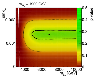
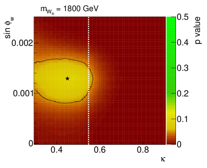
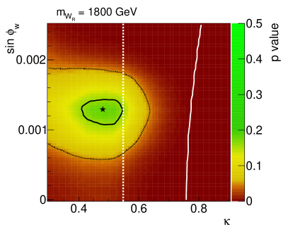
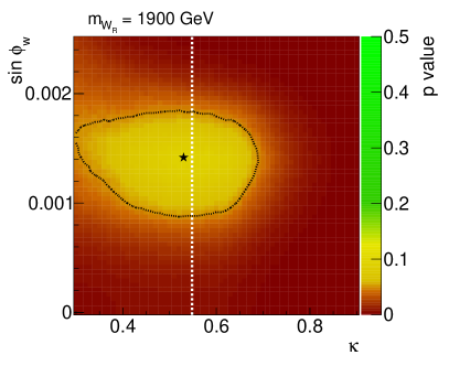
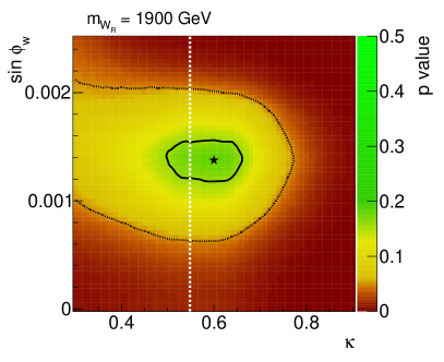
In Fig. 5 and 6 we present the results from our fit for and respectively. In the left panels we show the overall agreement with data when all experimental studies presented in the previous section are included. In this case, no part of the parameter space of the LRM is compatible with data at CL. This is due to the tension between the dijet excess in the ATLAS and CMS searches and the ATLAS search in the leptonic decay mode. However as we have argued in Sec. II.2, this ATLAS search finds a rate consistently below the background expectation, and while this does not lead to a strong CLs limit, it severely punishes the overall value in our fit for the full parameter space.
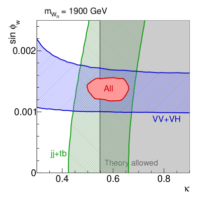
We therefore also present results where this single ATLAS search is excluded from the fit itself, where we explicitly check that the best-fit regions are not excluded by the CLs limits from this study. The results are shown in the right panels of Fig. 5 and 6. There is now a well-defined region where the LRM agrees very well with all searches and can describe the observed excess while satisfying the constraints from the other searches. For this region is roughly given by and . For the smaller production cross section allows for larger couplings and .
These preferred couplings fall into a special place in the parameter space: as described in Sec. III.1, the theory requires to be consistent. This means that for the preferred region at falls entirely in the unphysical regime. The situation is different in the scenario, where we find good agreement further from this boundary of the physically allowed region.
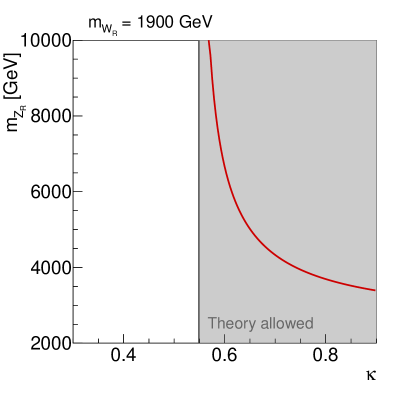
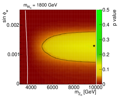
Since the mass of the is fixed by and (as shown in Eq. (8) and Fig. 4), we may also ask what mass the must have for the LRM to be consistent with the observations. A coupling close to the boundary corresponds to a very heavy , while large values of translate to lower masses. In Fig. 7 we show the results of our fit, still excluding the ATLAS leptonic search, in terms of and .
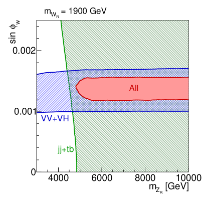
Assuming , the data permit a lower bound on of around 4 which is substantially above the masses probed so far at the LHC [38, 39, 40], . There is no upper bound on from our fit. This directly follows from the fact that our preferred regions for extend into the region , where becomes very large.
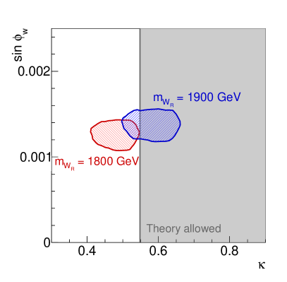
Our fit also allows us to analyze the origin of the constraints. In Fig. 8 we show the constraints from diboson and fermionic final states separately. As expected from Eq. (9) and (10), the dijet and rates fix the overall coupling constant while the and rates then set the mixing angle . We conclude this section with a comparison of the preferred regions for and in Fig. 9.
III.3 Prospects for Run II
As the LHC begins operations at 13 TeV, the prospects to discover or exclude the model presented here are excellent due to the steep rise in heavy particle production at higher energies. In this section we first estimate the amount of data that will be required to more thoroughly probe a possible resonance at 1.9 TeV. We then more speculatively explain the prospects that the LHC may produce and detect the neutral gauge boson.
At the 13 TeV LHC, the production cross-section for a resonance at 1.9 TeV is over 6 times higher than at 8 TeV. Consequently, if we assume that the background scales roughly in proportion with the signal, a mere 5 fb-1 will already probe the model in more detail than the current data set. Indeed, if no signal is observed, the dijet resonance search can already be expected to exclude our best-fit point at 95% CLs. This would also place the whole model under significant strain since it is the cross-section measurement that drives the overall coupling determination in our fit. If we do not see a continued excess here, the model is driven to couplings of unphysically small sizes for this value of the mass.
As Run II accumulates 10 fb-1, a signal should be observed in the final state otherwise the model assumption of flavour diagonal couplings will start to be under significant tension. On the gauge coupling side, our best fit model point can easily be excluded by both and searches with less than 15 fb-1.
A categorical 5 discovery does require larger data sets. Perhaps surprisingly given that most of the theoretical excitement has revolved around the diboson excesses, in our model we can expect the final state to be discovered first. Indeed, using the current search as a baseline, we expect a 5 discovery to be made with approximately 20 fb-1 if the current best-fit point is close to reality. A discovery in the final state would follow shortly afterwards with 30 fb-1. Again the gauge boson final states require more data with approximately 50 fb-1 required for confirmation of the final state, while over 100 fb-1 is expected to be required before is definitively seen.
More speculative is the discovery potential of the resonance since our model best fit point lies so close to a critical theory region. As explained in Sec. III.1, model consistency requires that , and depending on the mass assumed for the resonance, the best fit may be below this, see Fig. 5 and 6. The problem is that at as we head towards , the mass of the rapidly increases to a value far above the LHC collision energy.
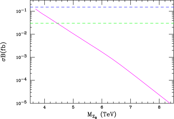
Nevertheless, there is still a region of the preferred fit value that allows for LHC relevant masses, especially if we assume GeV, see Fig. 9. A scenario with GeV is entirely possible and in Fig. 10 we give an estimation of the cross section at TeV as a function of . We find that the relevant region begins already to be probed once the LHC collects 20 fb-1 at 13 TeV. With 100 fb-1, the CLs exclusion region stretches to GeV.
IV A connection to dark matter?
An immediate question that arises when hints for new physics are found at the LHC is whether these hints could be connected to the physics of dark matter. In the context of the anomalies discussed in this paper, such a connection is not obvious. We will discuss four different scenarios in the following.
a) -mediated DM interactions with SM partners. If thermally produced DM particles are coupled to the SM sector through a resonance, they need a charged partner which they can annihilate into. could be a SM lepton, in particular the , but in this case the DM mass would have to be smaller than to forbid a fast DM decay via (the coupling of the to quarks is needed to explain the LHC anomalies discussed in the previous sections). In the context of the Left-Right Symmetric Model, could for instance be identified with the third generation right-handed neutrino. Then, however, mixing between and the other right-handed neutrinos must be forbidden or strongly suppressed to avoid fast decays into electrons and muons. Moreover, the -mediated annihilation cross section, which is of order
| (16) |
would be far below the generic value for a GeV thermal relic, cm3/sec [41]. In order to obtain the correct DM abundance in this case, significant entropy would need to be produced in the early Universe after DM freeze-out. While this is certainly possible, it would require a dark sector with a larger particle content and much richer dynamics than envisioned here. Alternatively, RH neutrino DM could be produced via a freeze-in mechanism. A scenario along these lines has been studied in Ref. [42].
b) -mediated DM interactions with charged partners beyond the SM. If both the and are new particles, a thermal freeze-out scenario is possible if the is heavier than the . Under this assumption, DM decay is forbidden, but freeze-out through - coannihilation in the early Universe is possible. Regarding the DM phenomenology today, neither direct detection nor indirect searches are expected to yield signals in this coannihilation scenario. At the LHC, however, DM could be detected in anomalous decays of the if . The process of interest is , where the 3-body decay proceeds through an off-shell . Possible search channels for this process are thus jets and missing transverse energy (MET), or the associated production of a top and bottom quark with MET. Both signatures are plagued by large SM backgrounds, mainly from vector boson + jets production, and it is hard to estimate their discovery potential without running full simulations. In addition, pair production would lead to final states involving multiple jets and MET, similar to typical signatures of supersymmetric models. Note that in this scenario the branching ratios of the into SM particles would be reduced compared to our assumptions in the previous sections, potentially allowing slightly larger values of to be consistent with data.
c) - and -mediated DM interactions. Since bosons typically come with neutral -like partners, it is also interesting to consider -mediated DM-SM interactions. We will do this in the context of the LRM discussed in Sec. III, but our conclusions easily generalize to other models, in particular to scenarios in which the LHC diboson anomaly is interpreted as being directly due to a resonance. The DM candidate could again be one of the standard right-handed neutrinos . In this case, however, we would again face the problem of fast DM decay through the . Therefore, let us consider a scenario where a new fermion multiplet with quantum number under is added to the model. The upper (neutral) component of this doublet is the DM candidate , the lower (charged) component is assumed to be sufficiently heavy for coannihilations to be negligible. Since the multiplet has the same quantum numbers as the right-handed leptons, there is the possibility of an undesirable mixing between and , which would reintroduce -mediated DM decay. Such mixing can be forbidden by introducing an additional symmetry, for instance a dark sector symmetry. Note that such a symmetry does not forbid a Majorana mass term for the , unlike for instance a symmetry. This is crucial, because if was a Dirac fermion, its vector couplings to the and (through gauge boson mixing) the would bring it into blatant conflict with direct detection results. For a Majorana DM particle, however, the dominant effect in direct detection experiments is spin-dependent scattering through axial vector interactions, for which limits are much weaker.
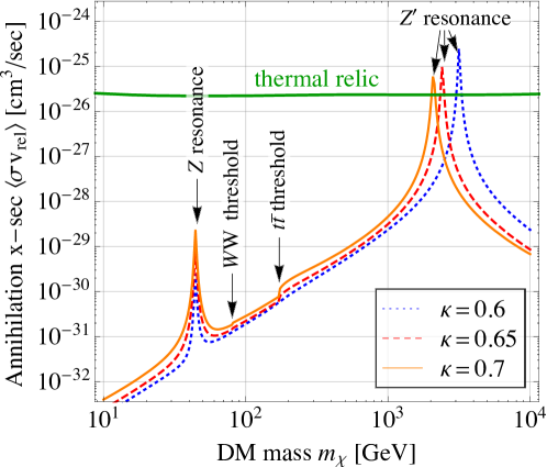
Annihilation of the in the early Universe proceeds through -channel and exchange into fermionic final states and into , with the fermionic final state dominating. This implies in particular that for or the total annihilation cross section is resonantly enhanced. Close to the resonance, the annihilation cross section to massless fermions is given by
| (17) |
Here , and are the vector and axial vector couplings of the final state fermions and the axial vector coupling of the DM particle to the , respectively. Explicit expressions for them have been given in Sec. III [32, 33]. Note that does not have vector couplings because it is a Majorana fermion. This the reason for the suppression in Eq. (17). It can be understood by noting that due to the Pauli exclusion principle, the two incoming DM particles can only be in an -wave state if their spins are opposite. The final state fermions are, however, produced in a spin-1 state due to the chirality structure of the gauge boson couplings. Thus, either one of them has to experience a helicity flip (which is only possible for ), or the initial state DM particles have to be in a -wave state. Note that in the resonance region, the -wave contribution proportional to is dominant. The reason is that, on resonance, an on-shell, spin-1 boson is produced, and this requires the DM particles to be in a spin-1 state as well. Outside the resonance region, the -wave terms dominate in the early Universe, where , while today, where in the Milky Way, it is the helicity-suppressed terms that give the main contribution.
This implies that the annihilation cross section today is several orders of magnitude below the thermal relic value, making indirect DM detection in this scenario extremely challenging.
To compute , we have used FeynCalc [43] to evaluate the annihilation cross sections for the and final states. Note that, in doing so, we need not only the coupling constants appearing in the simplified expression Eq. (17), but also the DM coupling to the SM-like boson. It is given by its coupling to the , multiplied by the - mixing angle as discussed in Sec. III. The coupling is at its SM value, while the coupling is again suppressed by a factor . Note that in evaluating the cross section for , we include only the transverse polarization states of the internal and external gauge bosons. Thus we avoid having to include model-dependent diagrams with Higgs boson exchange. Since annihilation to is subdominant by a large margin compared to annihilation to fermions, this approximation will not affect our results.
We plot as a function of the DM mass in Fig. 11 and compare it with the value required for a thermal relic [41]. Here we assume the conditions at DM freeze-out; in particular, we take for the average relative velocity of the two annihilating DM particles. We find that even at the resonance, the helicity and velocity suppression leads to annihilation cross section several orders of magnitude below the required value for the correct relic density. Only if the DM mass is close to mass, the resonant enhancement is large enough to make the annihilation cross section compatible with the observed relic density. On the other hand, this implies that, if the boson in this scenario is indeed responsible for the coupling of DM to the SM, the model provides a strong indication for the value of . Let us remark again that also an annihilation cross section somewhat below the naive thermal relic value may be acceptable if the Universe goes through a phase of extra entropy production after DM freeze-out, thus diluting the DM density.
It is also important to consider the dark matter–nucleon scattering cross section probed by direct detection experiments. Since is a Majorana particle with only axial vector couplings, the scattering will be spin-dependent. The cross section is
| (18) |
where or for scattering on protons and neutrons, respectively. As before, primed coupling constants denote couplings to the and unprimed ones indicate couplings to the . The hadronic form factors are taken from Ref. [44]. In Fig. 12 we show the cross section of DM interactions with protons as a function of the DM mass and of and compare it to limits from the XENON-100 [45] and PICO-2L [46] experiments. Independent of the DM mass, we find that our scenario predicts a cross section a few orders of magnitude below current exclusion bounds.
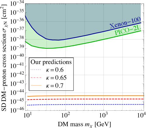
We can conclude that this simple scenario gives the correct relic density for DM close to the mass, while being fully consistent with current limits from direct detection experiments. Unfortunately, it is also not in reach of these experiments in the foreseeable future. We also expect the to be too heavy to be within the discovery reach of the LHC.
d) Minimal Left-Right Dark Matter. Another possibility for DM in the LRM is to introduce a pair of chiral fermion multiplets
| (19) |
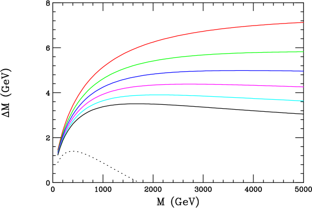
which share a common Majorana mass due to left-right exchange symmetry and whose neutral member(s) can be identified as DM. This scenario was recently considered in Ref. [47]. As was discussed there, such a scenario actually leads to a two-component picture for DM. Prior to electroweak radiative corrections, all members of the multiplets are degenerate. An issue that arises for the right-handed component is the sign of these corrections, i. e., whether or not they drive the masses of the charged states below that of that of the neutral member for some choice of the parameter ranges, in particular, the value of . Ref. [47] showed that for = 2 TeV and assuming one must have below TeV, otherwise this mass splitting goes negative thus preventing us from identifying the neutral component as (part of) DM. It thus behooves us to determine if this result is robust when we lower the value of to our range of interest. Employing the and couplings given above (as well as the general mass relationship), we find that the relevant mass splitting is now given by the expression
| (20) |
where and is given by the integral
| (21) |
which we can evaluate analytically111It is interesting to observe that the mass splitting vanishes in the case when all the mass functions, , are equal as it does in the case of the SM.. Fig. 13 shows the values we obtain for vs. as we vary over the relevant range as well as for the case of for comparison purposes always taking =1.9 TeV. Here we see that the mass splitting is always positive for the range of values of interest. We also observe that the magnitude of decreases as value increases. We note that at large masses, as increases, the curves begin to bend downward with an ever increasing slope. For the mass range shown here always remains positive until values of are reached.
e) DM in supersymmetric Left-Right models. A fifth possibility of introducing dark matter in the framework discussed here is to consider supersymmetric grand unified models based on Left-Right symmetry. In this case, the lightest neutralino is an excellent DM candidate, as has been extensively studied [48, 49]. However, its phenomenology is very similar to that of the lightest neutralino in the minimal supersymmetric standard model (MSSM), with no direct connection to the excesses seen at ATLAS and CMS.
V Conclusions
In this study we have analyzed the observed resonant excesses that appear in different ATLAS and CMS search channels in the invariant mass region of 1.8 – 2.0 TeV. The most prominent of these displays a excess in the search for the hadronic decay of a final state, though this peak is also sensitive to other diboson states. Both ATLAS and CMS find excesses in the dijet distributions at approximately the same mass, with a significance around and . There are further potential signals in CMS searches for semileptonic decays of vector boson pairs as well as for resonances decaying to a pair, significant at and . We have investigated potential scenarios that can explain these excesses while being consistent with all constraints from other searches.
In the first part of our analysis, we have performed a model-independent fit of the cross sections corresponding to the observed and expected event numbers in all searches from ATLAS and CMS that are sensitive to these and closely related final states, including the analyses that agree with background expectations. Our fit finds an overall tension between the SM and the data equivalent to . To explain the excess observed in vector boson pair production and associated Higgs production, a charged resonance is favoured over a neutral resonance. In particular, states decaying into pairs are strongly constrained from semileptonic searches. The best agreement is found for a charged resonance with approximately equal branching ratios into and pairs, with fitted signal cross sections around 5 fb in each final state. The excess in the dijet distributions suggest a branching ratio into quarks or gluons that is larger by a factor of at least 10, which is welcome news, as a sizable coupling of the heavy resonance to quarks or gluons is necessary for a sufficiently large production cross section at the LHC. Resonance searches in the state do not observe an excess, but the upper limit still allows a decay into this channel of approximately half the size of the dijet branching fraction.
As a next step, we have interpreted these signatures in the context of the Left-Right Symmetric Model based on the extended gauge group as the resonance production of a new heavy charged gauge boson, . Fitting this model to the data, we have found that a of 1900 GeV is in good agreement with all analyses, if the right-handed coupling is in the range and the mixing between the and is of the order . This preferred region can be translated into mass constraints for the associated heavy neutral gauge boson , for which we find a lower bound of approximately TeV. For a lighter , the bounds from the fit become stronger, requiring a smaller coupling and a heavier .
In the upcoming 13 TeV run, the LHC will be able to probe this potential signal with very little data. Already with an integrated luminosity of 5 fb-1, the experiments should be able to exclude the dijet signal of our best-fit scenario, followed by sensitivity in the channel shortly thereafter and then in the diboson channels with statistics of roughly 15 fb-1. For a discovery, we estimate that a luminosity of 20 fb-1 is needed in the channel, while the and especially the and states require more statistics. Whether the 13 TeV LHC will be able to produce the crucially depends on the value of (or equivalently ). The LHC will begin to probe the interesting parameter space for the new neutral gauge boson with integrated luminosities around 20 fb-1, but it is possible that this gauge boson is too heavy to be accessible at the 13 TeV LHC.
In addition, we have analyzed if this model can simultaneously explain dark matter. If the DM annihilates primarily through the , we require two new states, one charged and one neutral (the DM candidate). These would have to be relatively close in mass in order to be able to coannihilate and produce the correct relic density. In the case of a mediator, we introduce a new fermionic doublet with a neutral component to act as the dark matter. Here we find that a resonant mechanism is required to produce the correct amount of dark matter and thus if this solution is realized in nature, we predict the mass .
The fact that a number of excesses in different search channels across two experiments can be explained by an existing, simple (and, some might argue, natural) extension of the Standard Model is exciting. After the first months of data taking at the LHC at 13 TeV we will know more. We eagerly await the discovery of symmetry restoration in the upcoming operations of the 13 TeV LHC!
Note
Acknowledgements
We would like to express our gratitude to Tilman Plehn for encouragement to study the experimental excesses in more detail, as well as for collaboration in the early stages of the project. We wish to especially thank Gustaaf Brooijmans, David Morse and Chris Pollard for detailed discussions regarding the experimental results. We would also like to thank Felix Yu for useful discussions. In addition, we are grateful to Benjamin Fuks for providing a FeynRules implementation of the model. The authors would also like to thank the organizers of the Les Houches workshop, where part of this work was completed.
J. B., J. K., and J. T. would like to thank the kind support of the German Research Foundation (DFG) as part of the Forschergruppe ‘New Physics at the Large Hadron Collider’ (FOR 2239), J. B. also as part of the Graduiertenkolleg ‘Particle physics beyond the Standard Model’ (GRK 1940). The work of J. H and T. R. was supported by the Department of Energy, Contract DE-AC02-76SF00515. J. K. is supported by the DFG under Grant No. KO 4820/1–1.
Appendix A Fit input data
In Sec. II we have described a cross-section fit to all ATLAS and CMS analyses sensitive to diboson, , dijet and final states. This fit is based on a cut-and-count analysis in the mass bins around 1800 GeV. In Tbl. 9 we give the input information our fit uses in more detail, including the exact selections and mass bins that were used and the number of observed and expected background events in these analyses. Where available, these numbers are based on the papers, conference notes, supplementary material, and HepData entries published by ATLAS and CMS. Missing pieces of information were roughly estimated based on the available information. In some cases the estimated signal efficiencies and uncertainties were rescaled to give better agreement with the limits published by ATLAS and CMS, but we checked that this modification does not affect the overall fit results significiantly.
In analyses involving hadronic decays of gauge bosons, in particular in the ATLAS diboson search [1], bosons can be reconstructed in the selection and vice versa. Based on Fig. 1 c) in [1] we estimate this spill factor to be
| (22) |
The , and selections in [1] are not orthogonal. In fact, in the enlarged signal region there are only 2 observed events that are tagged in either of the or selections, but not in the category (see Fig. 13 of the auxiliary material published with [1]). This is why for the statistical combination of different searches we follow a conservative approach and only include the results from the selection.
| Fit input data | |||||||
|---|---|---|---|---|---|---|---|
| Analysis | Selection | Mass bins [GeV] | Obs. | Bkg. | (unc.) | Eff. | (unc.) |
| ATLAS hadronic [1] | selection | 1750 – 2050 | 13 | 8.5 | 1.3 | 0.10 | 0.04 |
| ATLAS hadronic [1] | selection | 1750 – 2050 | 9 | 3.0 | 0.8 | 0.08 | 0.02 |
| ATLAS hadronic [1] | selection | 1750 – 2050 | 18 | 10.0 | 1.5 | 0.09 | 0.03 |
| CMS hadronic [9] | Double tagged | 1780 – 2030 | 108 | 96.4 | 5.0 | 0.22 | 0.04 |
| ATLAS , single lepton [6] | Merged region | 1700 – 2000 | 8 | 9.1 | 5.2 | 0.27 | 0.01 |
| CMS , single lepton [5] | High purity | 1700 – 2000 | 12 | 12.3 | 5.3 | 0.26 | 0.03 |
| ATLAS , double lepton [7] | Merged region | 1680 – 2060 | 1 | 0.5 | 0.1 | 0.24 | 0.03 |
| CMS , double lepton [5] | High purity | 1700 – 2000 | 7 | 3.5 | 0.4 | 0.41 | 0.06 |
| CMS [4] | 1700 – 2000 | 3 | 0.5 | 0.4 | 0.06 | 0.01 | |
| CMS + hadronic vector [10] | 1500 – 2000 | 8 | 8.3 | 3.5 | 0.37 | 0.05 | |
| CMS , hadronic Higgs [11] | selection | 1690 – 2030 | 28 | 27.1 | 4.1 | 0.16 | 0.03 |
| ATLAS dijet [3] | 1706 – 2030 | 38326 | 37998 | 90.0 | 0.16 | 0.02 | |
| CMS dijet [2] | 1678 – 1945 | 114117 | 113438 | 100.0 | 0.38 | 0.04 | |
| ATLAS , hadronic [12] | Double tagged | 1600 – 2000 | 432 | 410.6 | 28.0 | 0.05 | 0.02 |
| ATLAS , leptonic [13] | 1600 – 2000 | 14 | 31.5 | 16.9 | 0.06 | 0.02 | |
| CMS , leptonic [14] | 1500 – 2000 | 178 | 187 | 20.0 | 0.13 | 0.01 | |
References
- Aad et al. [2015a] G. Aad et al. (ATLAS), (2015a), arXiv:1506.00962 [hep-ex] .
- Khachatryan et al. [2015a] V. Khachatryan et al. (CMS), Phys.Rev. D91, 052009 (2015a), arXiv:1501.04198 [hep-ex] .
- Aad et al. [2015b] G. Aad et al. (ATLAS), Phys.Rev. D91, 052007 (2015b), arXiv:1407.1376 [hep-ex] .
- Khachatryan et al. [2015b] V. Khachatryan et al. (CMS), CONF-Note CMS-PAS-EXO-14-010 (2015b).
- Khachatryan et al. [2014a] V. Khachatryan et al. (CMS), JHEP 1408, 174 (2014a), arXiv:1405.3447 [hep-ex] .
- Aad et al. [2015c] G. Aad et al. (ATLAS), Eur.Phys.J. C75, 209 (2015c), arXiv:1503.04677 [hep-ex] .
- Aad et al. [2015d] G. Aad et al. (ATLAS), Eur.Phys.J. C75, 69 (2015d), arXiv:1409.6190 [hep-ex] .
- Aad et al. [2015e] G. Aad et al. (ATLAS), Eur.Phys.J. C75, 263 (2015e), arXiv:1503.08089 [hep-ex] .
- Khachatryan et al. [2014b] V. Khachatryan et al. (CMS), JHEP 1408, 173 (2014b), arXiv:1405.1994 [hep-ex] .
- Khachatryan et al. [2015c] V. Khachatryan et al. (CMS), (2015c), arXiv:1502.04994 [hep-ex] .
- Khachatryan et al. [2015d] V. Khachatryan et al. (CMS), (2015d), arXiv:1506.01443 [hep-ex] .
- Aad et al. [2015f] G. Aad et al. (ATLAS), Eur.Phys.J. C75, 165 (2015f), arXiv:1408.0886 [hep-ex] .
- Aad et al. [2015g] G. Aad et al. (ATLAS), Phys.Lett. B743, 235 (2015g), arXiv:1410.4103 [hep-ex] .
- Chatrchyan et al. [2014] S. Chatrchyan et al. (CMS), JHEP 1405, 108 (2014), arXiv:1402.2176 [hep-ex] .
- Pati and Salam [1974] J. C. Pati and A. Salam, Phys.Rev. D10, 275 (1974).
- Mohapatra and Pati [1975a] R. N. Mohapatra and J. C. Pati, Phys.Rev. D11, 566 (1975a).
- Mohapatra and Pati [1975b] R. Mohapatra and J. C. Pati, Phys.Rev. D11, 2558 (1975b).
- Senjanovic and Mohapatra [1975] G. Senjanovic and R. N. Mohapatra, Phys.Rev. D12, 1502 (1975).
- Mohapatra [1986] R. Mohapatra, (1986), 10.1007/978-1-4757-1928-4.
- Langacker [1981] P. Langacker, Phys.Rept. 72, 185 (1981).
- Hewett and Rizzo [1989] J. L. Hewett and T. G. Rizzo, Phys.Rept. 183, 193 (1989).
- Read [2002] A. L. Read, J.Phys.G 28, 2693 (2002).
- Khachatryan et al. [2014c] V. Khachatryan et al. (CMS), Eur.Phys.J. C74, 3149 (2014c), arXiv:1407.3683 [hep-ex] .
- Deppisch et al. [2014] F. F. Deppisch, T. E. Gonzalo, S. Patra, N. Sahu, and U. Sarkar, Phys.Rev. D90, 053014 (2014), arXiv:1407.5384 [hep-ph] .
- Deppisch et al. [2015] F. F. Deppisch, T. E. Gonzalo, S. Patra, N. Sahu, and U. Sarkar, Phys.Rev. D91, 015018 (2015), arXiv:1410.6427 [hep-ph] .
- Heikinheimo et al. [2014] M. Heikinheimo, M. Raidal, and C. Spethmann, Eur.Phys.J. C74, 3107 (2014), arXiv:1407.6908 [hep-ph] .
- Dobrescu and Liu [2015a] B. A. Dobrescu and Z. Liu, (2015a), arXiv:1506.06736 [hep-ph] .
- Gluza and Jelinski [2015] J. Gluza and T. Jelinski, (2015), arXiv:1504.05568 [hep-ph] .
- Inami and Lim [1981] T. Inami and C. Lim, Prog.Theor.Phys. 65, 297 (1981).
- Adam et al. [2013] J. Adam et al. (MEG), Phys.Rev.Lett. 110, 201801 (2013), arXiv:1303.0754 [hep-ex] .
- Branco et al. [2012] G. C. Branco, P. M. Ferreira, L. Lavoura, M. N. Rebelo, M. Sher, and J. P. Silva, Phys. Rept. 516, 1 (2012), arXiv:1106.0034 [hep-ph] .
- Rizzo and Senjanovic [1981a] T. G. Rizzo and G. Senjanovic, Phys.Rev. D24, 704 (1981a).
- Rizzo and Senjanovic [1981b] T. G. Rizzo and G. Senjanovic, Phys.Rev.Lett. 46, 1315 (1981b).
- Deshpande et al. [1988] N. G. Deshpande, J. A. Grifols, and A. Mendez, Phys. Lett. B208, 141 (1988), [Erratum: Phys. Lett.B214,661(1988)].
- Dobrescu and Liu [2015b] B. A. Dobrescu and Z. Liu, (2015b), arXiv:1507.01923 [hep-ph] .
- Harland-Lang et al. [2015] L. Harland-Lang, A. Martin, P. Motylinski, and R. Thorne, Eur.Phys.J. C75, 204 (2015), arXiv:1412.3989 [hep-ph] .
- Melnikov and Petriello [2006] K. Melnikov and F. Petriello, Phys.Rev. D74, 114017 (2006), arXiv:hep-ph/0609070 [hep-ph] .
- Aad et al. [2014] G. Aad et al. (ATLAS), Phys.Rev. D90, 052005 (2014), arXiv:1405.4123 [hep-ex] .
- Khachatryan et al. [2015e] V. Khachatryan et al. (CMS), JHEP 1504, 025 (2015e), arXiv:1412.6302 [hep-ex] .
- Patra et al. [2015] S. Patra, F. S. Queiroz, and W. Rodejohann, (2015), arXiv:1506.03456 [hep-ph] .
- Steigman et al. [2012] G. Steigman, B. Dasgupta, and J. F. Beacom, Phys.Rev. D86, 023506 (2012), arXiv:1204.3622 [hep-ph] .
- Frere et al. [2007] J.-M. Frere, F.-S. Ling, L. Lopez Honorez, E. Nezri, Q. Swillens, et al., Phys.Rev. D75, 085017 (2007), arXiv:hep-ph/0610240 [hep-ph] .
- Mertig et al. [1991] R. Mertig, M. Bohm, and A. Denner, Comput.Phys.Commun. 64, 345 (1991).
- Belanger et al. [2009] G. Belanger, F. Boudjema, A. Pukhov, and A. Semenov, Comput.Phys.Commun. 180, 747 (2009), arXiv:0803.2360 [hep-ph] .
- Aprile et al. [2012] E. Aprile et al. (XENON100), Phys.Rev.Lett. 109, 181301 (2012), arXiv:1207.5988 [astro-ph.CO] .
- Amole et al. [2015] C. Amole et al. (PICO), Phys.Rev.Lett. 114, 231302 (2015), arXiv:1503.00008 [astro-ph.CO] .
- Heeck and Patra [2015] J. Heeck and S. Patra, (2015), arXiv:1507.01584 [hep-ph] .
- Bhattacharya et al. [2014] S. Bhattacharya, E. Ma, and D. Wegman, Eur.Phys.J. C74, 2902 (2014), arXiv:1308.4177 [hep-ph] .
- Esteves et al. [2012] J. Esteves, J. Romao, M. Hirsch, W. Porod, F. Staub, et al., JHEP 1201, 095 (2012), arXiv:1109.6478 [hep-ph] .
- Gao et al. [2015] Y. Gao, T. Ghosh, K. Sinha, and J.-H. Yu, (2015), arXiv:1506.07511 [hep-ph] .
- Cheung et al. [2015] K. Cheung, W.-Y. Keung, P.-Y. Tseng, and T.-C. Yuan, (2015), arXiv:1506.06064 [hep-ph] .
- Aguilar-Saavedra [2015] J. Aguilar-Saavedra, (2015), arXiv:1506.06739 [hep-ph] .
- Hisano et al. [2015] J. Hisano, N. Nagata, and Y. Omura, (2015), arXiv:1506.03931 [hep-ph] .
- Fukano et al. [2015] H. S. Fukano, M. Kurachi, S. Matsuzaki, K. Terashi, and K. Yamawaki, (2015), arXiv:1506.03751 [hep-ph] .
- Franzosi et al. [2015] D. B. Franzosi, M. T. Frandsen, and F. Sannino, (2015), arXiv:1506.04392 [hep-ph] .
- Xue [2015] S.-S. Xue, (2015), arXiv:1506.05994 [hep-ph] .
- Thamm et al. [2015] A. Thamm, R. Torre, and A. Wulzer, (2015), arXiv:1506.08688 [hep-ph] .