SImulator of GAlaxy Millimetre/submillimetre Emission (sígame ): CO emission from massive $z=2$ main-sequence galaxies

Abstract

We present sígame (SImulator of GAlaxy Millimetre/submillimetre Emission), a new numerical code designed to simulate the ¹²CO rotational line spectrum of galaxies. Using sub-grid physics recipes to post-process the outputs of smoothed particle hydrodynamics (SPH) simulations, a molecular gas phase is condensed out of the hot and partly ionised SPH gas. The gas is subjected to far-UV radiation fields and CR ionisation rates which are set to scale with the local star formation rate volume density. Level populations and radiative transport of the CO lines are solved with the 3-D radiative transfer code lime. We have applied sígame to cosmological SPH simulations of three disk galaxies at $z=2$ with stellar masses in the range $\sim 0.5-2\times 10^{11}$ $\rm{M}_{\odot}$ and star formation rates $\sim 40-140$ $\rm{M}_{\odot}$ yr^-1. Global CO luminosities and line ratios are in agreement with observations of disk galaxies at $z\sim 2$ up to and including $J=3-2$ but falling short of the few existing $J=5-4$ observations. The central $5\,{\rm kpc}$ regions of our galaxies have CO $3-2/1-0$ and $7-6/1-0$ brightness temperature ratios of $\sim 0.55-0.65$ and $\sim 0.02-0.08$, respectively, while further out in the disk the ratios drop to more quiescent values of $\sim 0.5$ and $<0.01$. Global CO-to-H₂ conversion ($\alpha_{\rm CO}$) factors are $\simeq 1.5\,{\rm\mbox{$\rm{M}_{\odot}$}\,pc^{-2}\,(K\,km\,s^{-1})^{-1}}$, i.e., $\sim 2-3\times$ below the typically adopted values for disk galaxies, and $\alpha_{\rm CO}$ increases with radius, in agreement with observations of nearby galaxies. Adopting a top-heavy Giant Molecular Cloud (GMC) mass spectrum does not significantly change the results. Steepening the GMC density profiles leads to higher global line ratios for $J_{\rm up}\geq 3$ and CO-to-H₂ conversion factors ($\simeq 3.6\,{\rm\mbox{$\rm{M}_{\odot}$}\,pc^{-2}\,(K\,km\,s^{-1})^{-1}}$).

1 Introduction

Inferring the physical properties of the molecular gas in galaxies is an important prerequisite for understanding their star formation. Carbon monoxide (CO) has proven to be a valuable tracer of the molecular interstellar medium (ISM), its rotational transitions being sensitive to a range of gas densities and temperatures through collisional excitation by H₂. Observations of CO lines have therefore been used extensively to probe the conditions of the molecular ISM in galaxies at high and low redshifts. However, the number of $z>1$ galaxies detected in CO is still relatively modest – little more than about 200 at the time of writing – with only a fraction of those having multiple CO transitions observed (see review by Carilli & Walter, 2013). Furthermore, the vast majority of high-$z$ CO measurements are of extreme objects such as submillimetre-selected galaxies (SMGs, see Frayer et al., 1998; Neri et al., 2003; Bothwell et al., 2013; Yun et al., 2015) and powerful QSOs with infra-red luminosities in excess of $10^{12}\,{\rm\mbox{$L_{\odot}$}}$ (Barvainis et al., 1994; Weiß et al., 2007; Riechers et al., 2011). Very few normal star forming galaxies at high redshifts, i.e., galaxies on the galaxy ‘main sequence’ (MS), have been observed in CO to date, and as a result little is known, however, about the ISM conditions of normal star-forming galaxies at high redshifts. Some of the best studied cases are the four BzK-selected galaxies BzK$-$4171, BzK$-$16000, and BzK$-$21000 at $z\simeq 1.5$, where up to four CO transitions, including CO(1$-$0), have been observed (Dannerbauer et al., 2009; Aravena et al., 2010; Daddi et al., 2015). While the initial analysis of the low-$J$ ($J_{\rm up}\leq 3$) transitions in these galaxies suggested a quiescent ISM reminiscent of the Milky Way (MW) (Dannerbauer et al., 2009), the more recent CO$(5-4)$ observations require a second much denser, and likely warmer, ISM component, which is thought to be directly associated with star forming clumps within the galaxies (Daddi et al., 2015). Studies such as these illustrate the importance of sampling both the low- and high-$J$ parts of the CO Spectral Line Energy Distribution (SLED) in order to obtain a comprehensive picture of the molecular gas in galaxies.

With the Atacama Large Millimetre/submillimetre Array (ALMA) now in operation, the collection of CO data is gaining rapid pace as is our understanding of the molecular gas in distant galaxies. Galaxy evolution simulations that include molecular line emission (such as CO) are an important tool with which to interpret the observed molecular emission of galaxies caught in various evolutionary stages. The past decade saw the development of the first detailed simulations of CO line emission from galaxies, which consisted of SPH galaxy simulations (Narayanan et al., 2006; Narayanan et al., 2011; Narayanan & Krumholz, 2014; Greve & Sommer-Larsen, 2008), or semi-analytical models (Obreschkow et al., 2009, 2011; Lagos et al., 2012; Muñoz & Furlanetto, 2013; Popping et al., 2014), combined with sub-grid physics prescriptions to model the molecular gas phase and its CO content. The simulations were used to examine the CO emission properties of high-$z$ mergers and starbursts (Narayanan et al., 2008c, 2009), active galactic nuclei (AGN) and quasars (Narayanan et al., 2006, 2008b, 2008a), as well as moderately star-forming galaxies (Greve & Sommer-Larsen, 2008; Narayanan et al., 2011; Lagos et al., 2012; Popping et al., 2014). For example, simulating a large set of galaxies, Narayanan & Krumholz (2014) proposed a calibration scheme in which the global CO SLED is parameterised by the star formation rate (SFR) surface density, the latter being a more readily observed quantity. Simulations of CO have also been used to examined how well CO can probe the relationship between gas surface density and SFR, i.e., the so-called Kennicutt-Scmidt relations, and the validity of the CO-to-H₂ conversion factor ($X_{\rm CO}$) used to infer H₂ column densities from measured CO $J=1-0$ line intensities (e.g., Narayanan et al., 2011; Narayanan & Hopkins, 2013).

Here we present a new numerical framework for simulating the molecular line emission from star-forming galaxies. The code, SImulator of GAlaxy Millimetre/submillimetre Emission (sígame), combines SPH (or grid-based) simulations of galaxies with sub-grid physics prescriptions for the H₂/Hi fraction and the ISM thermal balance on scales of individual Giant Molecular Clouds (GMCs). sígame accounts for a FUV and cosmic ray (CR) intensity field that vary with local SFR density within the galaxy. In this paper, we apply sígame to cosmological SPH simulations of three massive, normal star-forming galaxies at $z=2$ (i.e., so-called main-sequence galaxies), and model their CO rotational line spectrum using a publicly available 3D radiative transfer code. We show that sígame reproduces observed low-$J$ CO line luminosities and provides new estimates of the $\alpha_{\rm CO}$ factor for main-sequence galaxies at $z\sim 2$, while at the same time predicting their CO line luminosities at high-$J$ ($J_{\rm up}>6$) transitions where observations are yet to be made.

The structure of the paper is as follows. Section $2$ describes the cosmological SPH simulations used, along with the basic properties of the three $z=2$ star-forming galaxies extracted from the simulations. A detailed description of sígame and its application to the three simulations is presented in Section $3$, along with a bench test of the code on MW-like galaxies at $z=0$. The resulting CO emission maps and SLEDs of the $z=2$ simulations are presented in Section $4$, and compared to CO observations of similar galaxies at $z\sim 1-2.5$. In section $5$, we explore how the results in Section $4$ change when adopting alternative ISM models. Section $6$ discusses the strengths and weaknesses of sígame in the context of other molecular line (CO) simulations and recent observations. Finally, in Section $7$ we summarise the main steps of sígame, and list our main findings regarding the CO line emission from massive, star-forming galaxies at $z\simeq 2$. We adopt a flat cold dark matter ($\Lambda$CDM) scenario with $\Omega_{m}=0.3$, $\Omega_{\Lambda}=0.7$ and $h=0.65$ (Planck Collaboration XVI, 2014).

2 Cosmological Simulations

2.1 SPH simulations

We employ a cosmological TreeSPH code for simulating galaxy formation and evolution, though in principle, grid-based hydrodynamic simulations could be incorporated equally well. The TreeSPH code used for the simulations is in most respects similar to the one described in Sommer-Larsen et al. (2005) and Romeo et al. (2006). A cosmic baryon fraction of $f_{\rm{b}}=0.15$ is assumed, and simulations are initiated at a redshift of $z=39$. The implementation of star formation and stellar feedback, however, has been manifestly changed.

Star formation is assumed to take place in cold gas ($\mbox{$T_{\rm{k}}$}\la 10^{4}$ K) at densities $\mbox{$n_{\rm{H}}$}>1$ cm^-3. The star formation efficiency (or probability that a gas particle will form stars) is formally set to 0.1, but is, due to effects of self-regulation, considerably lower. Star formation takes place in a stochastic way, and in a star formation event, $1$ SPH gas particle is converted completely into $1$ stellar SPH particle, representing the instantaneous birth of a population of stars according to a Chabrier (2003) stellar initial mass function (IMF; Chabrier 2003) – see further below.

The implementation of stellar feedback is based on a sub-grid super-wind model, somewhat similar to the ‘high-feedback’ models by Stinson et al. (2006). These models, though, build on a supernova blast-wave approach rather than super-wind models. Both types of models invoke a Chabrier (2003) IMF, which is somewhat more top-heavy in terms of energy and heavy-element feedback than, e.g., the standard Salpeter IMF. The present models result in galaxies characterised by reasonable $z=0$ cold gas fractions, abundances and circum-galactic medium abundance properties. They also improve considerably on the “angular momentum problem” relative to the models presented in, e.g., Sommer-Larsen et al. (2003). The models will be described in detail in a forthcoming paper.

2.2 The model galaxies

Three model galaxies, hereafter referred to as G1, G2 and G3 in order of increasing SFR, were extracted from the above SPH simulation and re-simulated using the ‘zoom-in’ technique described in (e.g., Sommer-Larsen et al., 2003). The emphasis in this paper is on massive ($M_{*}\gtrsim 5\times 10^{10}\,\mbox{$\rm{M}_{\odot}$}$) galaxies, and the three galaxies analysed are therefore larger, rescaled versions of galaxies formed in the 10/$h$ Mpc cosmological simulation described in Sommer-Larsen et al. (2003). The linear scale-factor is of the order 1.5, and since the CDM power spectrum is fairly constant over this limited mass range the rescaling is a reasonable approximation.

Galaxy G1 was simulated at fairly high resolution, using a total of $1.2\times 10^{6}$ SPH and dark matter particles, while about $9\times 10^{5}$ and $1.1\times 10^{6}$ particles were used in the simulations of G2 and G3, respectively. For the G1 simulation, the masses of individual SPH gas, stellar and dark matter particles are $m_{\rm{SPH}}=m_{*}\approx 6.3\times 10^{5}$ $h^{-1}$M_⊙ and $m_{\rm{DM}}$=$3.5\times 10^{6}$ $h^{-1}$M_⊙, respectively. Gravitational (cubic spline) softening lengths of 310, 310 and 560 $h^{-1}$pc, respectively, were employed. Minimum gas smoothing lengths were about $50\,h^{-1}$pc. For the lower resolution simulations of galaxies G2 and G3, the corresponding particle masses are $m_{\rm{SPH}}=m_{*}\approx 4.7\times 10^{6}$ $h^{-1}$M_⊙ and $m_{\rm{DM}}=2.6\times 10^{7}$ $h^{-1}$M_⊙, respectively, and the gravitational softening lengths were 610, 610 and 1090 $h^{-1}$pc. Minimum gas smoothing lengths were about 100 $h^{-1}$pc.

Figure 1: SPH gas surface density maps of the three model galaxies G1 (top), G2 (middle), and G3 (bottom) viewed face-on. The stellar masses and SFRs of each galaxy are indicated (see also Table 1). The maps have been rendered with the visualization tool SPLASH version 2.4.0 (Price, 2007) using the gas smoothing lengths provided by the simulations.

Due to effects of gravitational softening, typical velocities in the innermost parts of the galaxies (typically at radii less than about 2$\epsilon_{\rm{SPH}}$, where $\epsilon_{\rm{SPH}}$ is the SPH and star particle gravitational softening length) are somewhat below dynamical values (see, e.g. Sommer-Larsen et al., 1998). The dynamical velocities will be of the order $v_{\rm{dyn}}=\sqrt{GM(R)/R}$, where $G$ is the gravitational constant, $R$ is the radial distance from the centre of the galaxy and $M(R)$ is the total mass located inside of $R$. Indeed, it turns out that for the simulated galaxies considered in this paper SPH particle velocities inside of 2$\epsilon_{\rm{SPH}}$ are only about 60-70% of what should be expected from dynamics. To coarsely correct for this adverse numerical effect, for SPH particles inside of 2$\epsilon_{\rm{SPH}}$ the velocities are corrected as follows: For SPH particles of total velocity less than $v_{\rm{dyn}}$, the tangential component of the velocity is increased such that the total velocity becomes equal to $v_{\rm{dyn}}$. Only the tangential component is increased in order not to create spurious signatures of merging. With this correction implemented, the average ratio of total space velocity to dynamical velocity of all SPH particles inside of 2$\epsilon_{\rm{SPH}}$ equals unity.

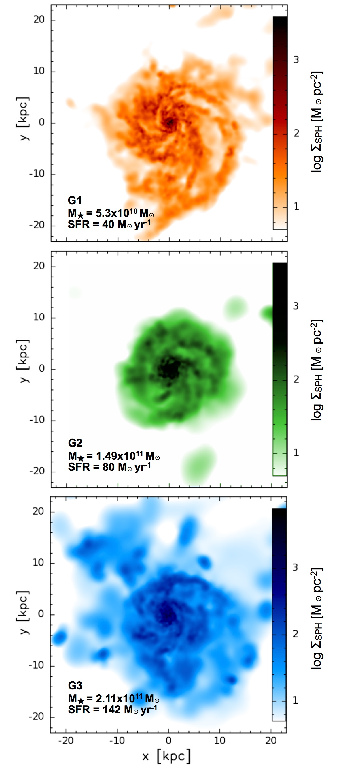
Figure 1 shows surface density maps of the SPH gas in G1, G2, and G3, i.e., prior to any post-processing by sígame. The gas is seen to be strongly concentrated towards the centre of each galaxy and structured in spiral arms containing clumps of denser gas. The spiral arms reach out to a radius of about $20$ kpc in G1 and G3, with G2 showing a more compact structure that does not exceed $R\sim 15$ kpc. Table 1 lists key properties of the simulated galaxies, namely their SFR, stellar mass ($M_{*}$), SPH gas mass ($M_{\rm SPH}$), SPH gas mass fraction ($f_{\rm SPH}=M_{\rm SPH}/(M_{*}+M_{\rm SPH})$), and metallicity $Z^{\prime}$. These quantities were measured within a radius ($R_{\rm cut}$, also given in Table 1) corresponding to where the radial cumulative stellar mass function has flattened out. The metallicity is in units of solar metallicity and is calculated from the abundances of C, N, O, Mg, Si, S, Ca and Fe in the SPH simulations, and adjusted for the fact that not all heavy metals have been included according to the solar element abundancies measured by Asplund et al. (2009).

Table 1: Physical properties of the three simulated galaxies G1, G2, and G3

	SFR	$M_{\ast}$	$M_{\rm SPH}$	$f_{\rm SPH}$	$Z^{\prime}$	$R_{\rm cut}$
	[$\rm{M}_{\odot}$ yr-1]	[$10^{11}\,\rm{M}_{\odot}$]	[$10^{10}\,\rm{M}_{\odot}$]			[kpc]
G1	40	$0.53$	$2.07$	28%	1.16	$20$
G2	80	$1.49$	$2.63$	15%	1.97	$15$
G3	142	$2.11$	$4.66$	18%	1.36	$20$

Notes. All quantities are determined within a radius $R_{\rm cut}$, which is the radius where the cumulative radial stellar mass function of each galaxy becomes flat. The gas mass ($M_{\rm SPH}$) is the total SPH gas mass within $R_{\rm cut}$. The metallicity ($\mbox{$Z^{\prime}$}=Z/Z_{\odot}$) is the mean of all SPH gas particles within $R_{\rm cut}$.

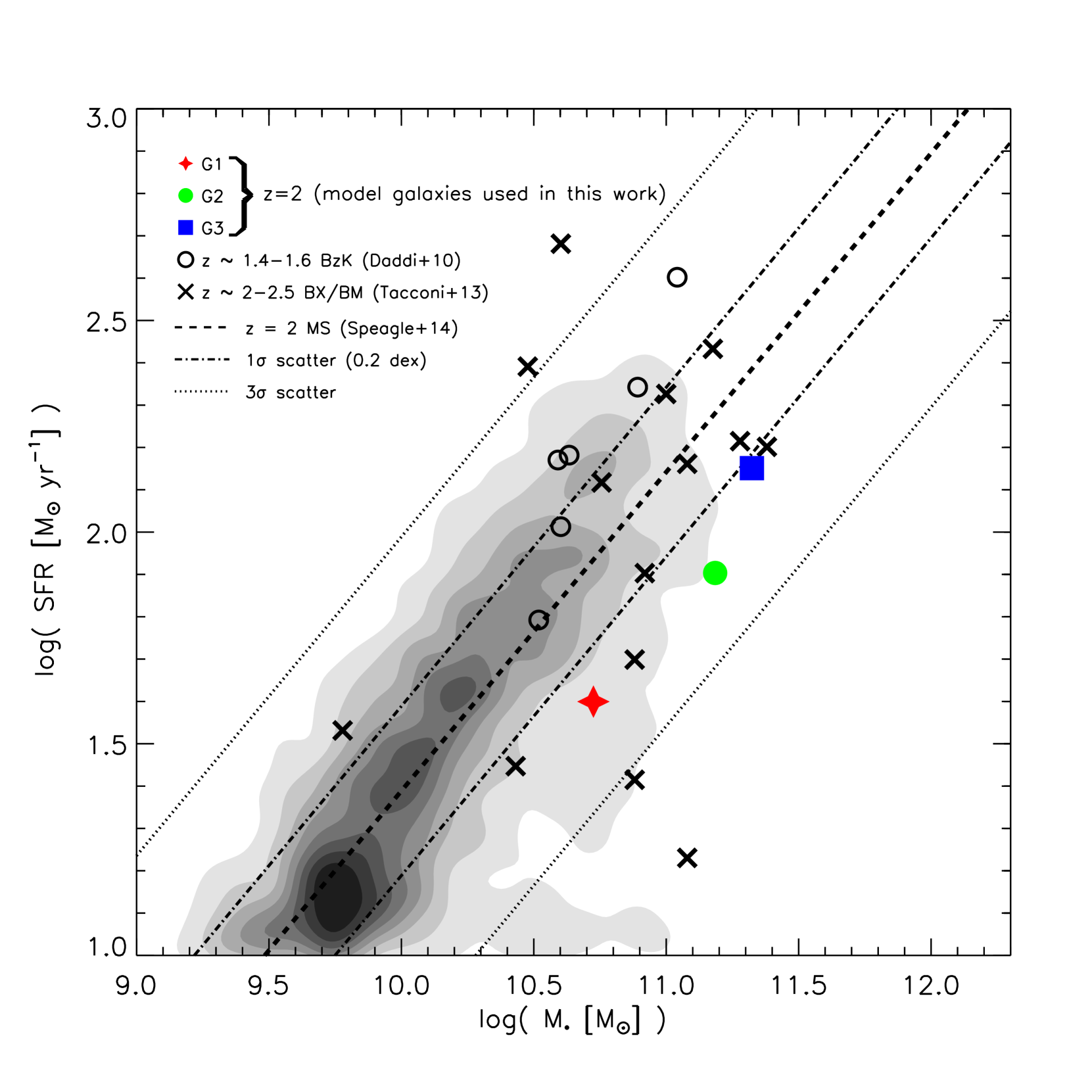
The location of our three model galaxies in the SFR-$M_{*}$ diagram is shown in Figure 2 along with a sample of 3754 $1.4<z<2.5$ main-sequence galaxies selected in near-IR from the NEWFIRM Medium-Band Survey (Whitaker et al., 2011). The latter used a Kroupa IMF but given its similarity with a Chabrier IMF no conversion in the stellar mass and SFR was made (cf., Papovich et al. (2011) and Zahid et al. (2012) who use conversion factors of 1.06 and 1.13, respectively). Also shown is the determination of the main-sequence relation at $z\simeq 2$ by Speagle et al. (2014), and the 1 and $3\sigma$ scatter around it. G1, G2, and G3 are seen to lie within the $3\sigma$ scatter around the $z\simeq 2$ main sequence, albeit offset somewhat towards lower SFRs. This latter tendency is also found among a subset of CO-detected BX/BM galaxies at $z\sim 2-2.5$ (Tacconi et al., 2013), highlighted in Figure 2 along with a handful of $z\sim 1.5$ BzK galaxies also detected in CO (Daddi et al., 2010). The BX/BM galaxies are selected by a UGR colour criteria (Adelberger et al., 2004), while the BzK galaxies are selected by the BzK colour criteria (Daddi et al., 2004). Based on the above we conclude that, in terms of stellar mass and SFR, our three model galaxies are representative of the star-forming galaxy population detected in CO at $z\sim 2$.

Figure 2: Position of the three model galaxies studied here (G1, G2 and G3 with filled a red star, a green circle and a blue square respectively), on a SFR–M_∗ diagram. The grey filled contours show the $z\sim 2$ number density of $3754$ $1.4<z<2.5$ galaxies from the NEWFIRM Medium-Band Survey (Whitaker et al., 2011). The ${\rm SFR-M_{\ast}}$ relation at $z\simeq 2$ as determined by Speagle et al. (2014) is indicated by the dashed line, with the $1\sigma$ and $3\sigma$ scatter of the relation shown by the dot-dashed and dotted lines, respectively. Also shown are six $z\sim 1.4-1.6$ BzK galaxies (black circles; Daddi et al. 2010) and 14 $z\sim 2-2.5$ Bx/BM galaxies (black crosses; Tacconi et al. 2013). The BzK galaxies are from top to bottom: BzK$-$12591, BzK$-$21000, BzK$-$16000, BzK$-$17999, BzK$-$4171 and BzK$-$2553 (following the naming convention of Daddi et al. 2010).

3 Modeling the ISM with sígame

3.1 Methodology overview

Here we give an overview of the major steps that go into sígame, along with a brief description of each. The full details of each step are given in subsequent sections and in appendices A through C. We stress, that sígame operates entirely in the post-processing stage of an SPH simulation, and can in principle easily be adapted to any given SPH galaxy simulation as long as certain basic quantities are known for each SPH particle in the simulation, namely: position ($\boldsymbol{r}$), velocity ($\vec{v}$), atomic hydrogen density ($n_{\rm{H}}$), metallicity ($Z^{\prime}$), kinetic temperature ($T_{\rm{k}}$), smoothing length ($h$), and star formation rate (SFR). The key steps involved in sígame are:

1. Cooling of the SPH gas. The initially hot ($T_{\rm k}\sim 10^{3-7}\,{\rm K}$) SPH gas particles are cooled to temperatures typical of the warm neutral medium ($\lesssim 10^{4}\,{\rm K}$) by atomic and ionic cooling lines primarily.

2. Inference of the molecular gas mass fraction ($\mbox{$f^{\prime}_{\rm mol}$}=m_{\rm H_{2}}/m_{\rm SPH}$) of each SPH particle after the initial cooling in step 1. $f^{\prime}_{\rm mol}$ for a given SPH particle is calculated by taking into account its temperature, metallicity, and the local CR and FUV radiation field impinging on it.

3. Distribution of the molecular gas into GMCs. Cloud masses and sizes are obtained from random sampling of the observed GMC mass-spectrum in nearby quiescent galaxies and applying the local GMC mass-size relation.

4. GMC thermal structure. A radial density profile is adopted for each GMC and used to calculate the temperature structure throughout individual clouds, taking into account heating and cooling mechanisms relevant for neutral and molecular gas, when exposed to the local CR and attenuated FUV fields.

5. Radiative transport of CO lines. Finally, the CO line spectra are calculated separately for each GMC with a radiative transfer code and accumulated on a common velocity axis for the entire galaxy.

Determining the temperature (i) and the molecular gas mass fraction (ii) of a warm neutral gas SPH particle cannot be done independently of each other, but must be solved for simultaneously in an iterative fashion (see Sections 3.2 and 3.3). As already mentioned, we shall apply sígame to the SPH simulations of galaxies G1, G2, and G3 described in Section 2, and in doing so we will use them to illustrate the workings of the code.

3.2 The Warm and Cold Neutral Medium

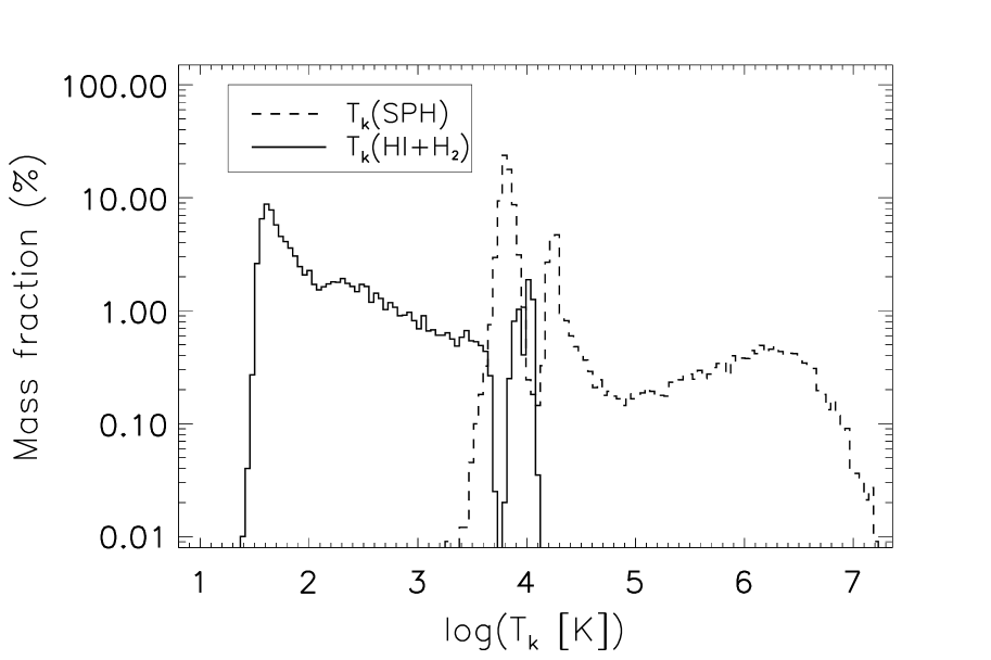
In SPH simulations of galaxies the gas is typically not cooled to temperatures below a few thousand Kelvin (Springel & Hernquist, 2003). This is illustrated in Figure 3, which shows the SPH gas temperature distribution (dashed histogram) in G1 (for clarity we have not shown the corresponding temperature distributions for G2 and G3, both of which are similar to that of G1). Minimum SPH gas temperatures in G1, G2 and G3 are about 1200 K, 3100 K and 3200 K, respectively, and while temperatures span the range $\sim 10^{3-7}\,{\rm K}$, the bulk ($\sim 80-90\%$) of the gas mass in all three galaxies is at $\mbox{$T_{\rm{k}}$}\lesssim 10^{5}\,{\rm K}$.

At these temperatures the gas will be in atomic or ionised form, and H atoms that attach to dust grain surfaces via chemical bonds (chemisorbed) will evaporate from the grains before H₂ can be formed. H₂ can effectively only exist at temperatures below $\sim 10^{3}$ K, assuming a realistic desorption energy of $3\times 10^{4}$ K for chemisorbed H atoms (see Cazaux & Spaans, 2004). The first step of sígame is therefore to cool some portion of the hot SPH gas down to $\mbox{$T_{\rm{k}}$}\lesssim 10^{3}\,{\rm K}$, i.e., a temperature range characteristic of a warm and cold neutral medium for which we can meaningfully employ a prescription for the formation of H₂.

sígame employs the standard cooling and heating mechanisms pertaining to a hot, partially ionised gas. Cooling occurs primarily via emission lines from H, He, C, O, N, Ne, Mg, Si, S, Ca, and Fe in their atomic and ionised states, with the relative importance of these radiative cooling lines depending on the temperature (Wiersma et al., 2009). In addition to these emission lines, electron recombination with ions can cool the gas, as recombining electrons take away kinetic energy from the plasma, a process which is important at temperatures $>10^{3}$ K (Wolfire et al., 2003). At similar high temperatures another important cooling mechanism is the scattering of free electrons off other free ions, whereby free-free emission removes energy from the gas (Draine, 2011). Working against the cooling is heating caused by cosmic rays via the expulsion of bound electrons from atoms or the direct kinetic transfer to free electrons via Coulomb interactions (Simnett & McDonald, 1969). By ignoring heating of the gas by photo-ionization, we shall adopt an assumption typically used for galactic ISM (Gnat & Sternberg, 2007; Smith et al., 2008), though see Wiersma et al. (2009) who demonstrate how cooling rates are reduced when including photoionization in the intergalactic medium and proto-galaxies.

We arrive at a first estimate of the temperature of the neutral medium by requiring energy rate equilibrium between the above mentioned heating and cooling mechanisms:

$$\mbox{$\Gamma_{\rm{CR,H}\textsc{i}}$}=\mbox{$\Lambda_{\rm{atoms+ions}}$}+\mbox{$\Lambda_{\rm{rec}}$}+\mbox{$\Lambda_{\rm{f-f}}$},$$ (1)

where $\Lambda_{\rm{atoms+ions}}$ is the cooling rate due to atomic and ionic emission lines, $\Lambda_{\rm{rec}}$ and $\Lambda_{\rm{f-f}}$ are the cooling rates from recombination processes and free-free emission as described above, and $\Gamma_{\rm{CR,H}\textsc{i}}$ is the CR heating rate in atomic, partly ionised, gas. The detailed analytical expressions employed by sígame for these heating and cooling rates are given in appendix A.

The abundances of the atoms and ions included in $\Lambda_{\rm{atoms+ions}}$ either have to be calculated in a self-consistent manner as part of the SPH simulation or set by hand. For our set of galaxies, the SPH simulations follow the abundances of H, C, N, O, Mg, Si, S, Ca and Fe, while for the abundances of He and Ne, we adopt solar mass fractions of $0.2806$ and $10^{-4}$, respectively, as used in Wiersma et al. (2009).

$\Gamma_{\rm{CR,H}\textsc{i}}$ depends on the primary CR ionization rate ($\zeta_{\rm{CR}}$), a quantity that is set by the number density of supernovae since they are thought to be the main source of CRs (Ackermann et al., 2013). In sígame, this is accounted for by parameterizing $\zeta_{\rm{CR}}$ as a function of the local star formation rate density (SFRD) as it varies across the simulated galaxy. The details of this parameterization are deferred to Section 3.4.3.

Figure 3: The distributions of gas kinetic temperature before (dashed histogram) and after (solid histogram) applying the heating and cooling mechanisms of eq. 1 to galaxy G1. The original hot SPH gas is seen to span a temperature range from about $10^{3}$ K up to $\sim 10^{7}$ K, while once the gas has been cooled the temperature distribution only barely exceeds $\sim 10^{4}$ K.

In eq. 1, all terms but $\Lambda_{\rm{atoms+ions}}$ depend on the ionization fraction ($x_{e}=n_{e}/n_{\rm HI}$) of the gas, which in turn depends on the total CR ionization rate (i.e., $\zeta_{\rm{CR}}$ corrected for secondary ionizations of H and He), the gas temperature ($T_{\rm{k}}$), and the H i density ($n_{\rm{H}\textsc{i}}$) (see appendix A). The ionization fraction is calculated taking into account the ionization of H and He (with a procedure kindly provided by I. Pelupessy; see also Pelupessy (2005)). Since, $n_{\rm{H}\textsc{i}}$ is set by the molecular gas mass fraction ($f^{\prime}_{\rm mol}$), which in turn also depends on $T_{\rm{k}}$ (see Section 3.3 on how $f^{\prime}_{\rm mol}$ is calculated), eq. 1 has to be solved in an iterative fashion until consistent values for $T_{\rm{k}}$, $n_{\rm{e}}$, and $f^{\prime}_{\rm mol}$ are reached. Example solutions are given in Figure 13 in Appendix A.

The temperature distribution that results from solving eq. 1 for every SPH particle in the G1 simulation is shown in Figure 3 (very similar distributions are obtained for G2 and G3). The gas has been cooled to $\mbox{$T_{\rm{k}}$}\lesssim 10^{4}$  K, with temperatures extending down to $\sim 25\,{\rm K}$. This new gas phase represents both the warm neutral medium (WNM) and the cold neutral medium (CNM), and from it we derive the molecular gas phase.

3.3 Hi to H₂ conversion

For the determination of the molecular gas mass fraction associated with each SPH gas particle we use the prescription of Pelupessy et al. (2006), inferred by equating the formation rate of H₂ on dust grains with the photodissociation rate of H₂ by Lyman-Werner band photons, and taking into account the self-shielding capacity of H₂ and dust extinction. We ignore H₂ production in the gas phase (cf., Christensen et al., 2012) since only in diffuse low metallicity ($\lesssim 0.1Z_{\odot}$) gas is this thought to be the dominant formation route (Norman & Spaans, 1997), and so should not be relevant in our model galaxies that have mean metallicities $\mbox{$Z^{\prime}$}>1$ (see Table 1) and very little gas with $\mbox{$Z^{\prime}$}<0.1$ (see Figure 15 in Appendix C). We adopt a steady-state for the H i$\rightarrow$H₂ transition, meaning that we ignore any time dependence owing to temporal changes in the UV field strength and/or disruptions of GMCs, both of which can occur on similar time scales as the H₂ formation. This has been shown to be a reasonable assumption for environments with metallicities $\gtrsim 0.01\,Z_{\odot}$ (Narayanan et al., 2011; Krumholz & Gnedin, 2011).

The first step is to derive the FUV field strength, $G_{0}^{\prime}$, which sets the H i$\rightarrow$H₂ equilibrium. In sígame, $G_{0}^{\prime}$ consists of a spatially varying component that scales with the local SFRD (${\rm SFRD_{local}}$) in different parts of the galaxy on top of a constant component set by the total stellar mass of the galaxy. This is motivated by Seon et al. (2011) who measured the average FUV field strength in the MW ($G^{\prime}_{\rm 0,MW}$) and found that about half comes from star light directly with the remainder coming from diffuse background light. We shall assume that in the MW the direct stellar contribution to $G^{\prime}_{\rm 0,MW}$ is determined by the average SFRD ($\rm SFRD_{MW}$), while the diffuse component is fixed by the stellar mass (${\rm M}_{*,\rm{MW}}$). From this assumption, i.e., by calibrating to MW values, we derive the desired scaling relation for $G_{0}^{\prime}$ in our simulations:

$$\mbox{$G_{0}^{\prime}$}=G^{\prime}_{\rm 0,MW}\left(0.5\frac{{\rm SFRD}_{\rm{local}}}{{\rm SFRD}_{\rm{MW}}}+0.5\frac{{\rm M}_{*}}{{\rm M}_{\rm*,MW}}\right),$$ (2)

where $G^{\prime}_{\rm 0,MW}=0.6$ Habing (Seon et al., 2011), and ${\rm M}_{*,\rm{MW}}=6\times 10^{10}$  $\rm{M}_{\odot}$ (McMillan, 2011). For ${\rm SFRD}_{\rm{MW}}$ we adopt $0.0024$ $\rm{M}_{\odot}$ yr^-1  kpc^-3, inferred from the average SFR within the central 10 kpc of the MW ($0.3$ $\rm{M}_{\odot}$ yr^-1; Heiderman et al., 2010) and within a column of height equal to the scale height of the young stellar disk ($0.2\,{\rm kpc}$; Bovy et al., 2012) of the MW disk. ${\rm SFRD_{local}}$ is the SFRD ascribed to a given SPH particle, and is calculated as the volume-averaged SFR of all SPH particles within a $5\,{\rm kpc}$ radius. Note, that the stellar mass sets a lower limit on $G_{0}^{\prime}$, which for G1, G2, and G3 are $0.22$, $0.62$, and $0.88$ Habing, respectively.

Next, the gas upon which the FUV field impinges is assumed to reside in logotropic clouds, i.e., clouds with radial density profiles given by $n(r)=\mbox{$n_{\rm{H,ext}}$}\left(r/R\right)^{-1}$, where $n_{\rm{H,ext}}$ is the density at the cloud radius $R$. For a logotropic density profile, the external density is given by $n_{\rm{H,ext}}=2/3\langle\mbox{$n_{\rm{H}}$}\rangle$, where we approximate $\langle\mbox{$n_{\rm{H}}$}\rangle$ with the original SPH gas density. From Pelupessy et al. (2006) we then have that the molecular gas mass fraction, including heavier elements than hydrogen, of each cloud is given by:

$$\mbox{$f^{\prime}_{\rm mol}$}\equiv\frac{m_{\rm mol}}{m_{\rm SPH}}=\exp{\left[-4\frac{\mbox{$A_{\rm{v}}^{\rm{(tr)}}$}}{\langle\mbox{$A_{\rm{v}}$}\rangle}\right]}.$$ (3)

Here $\langle\mbox{$A_{\rm{v}}$}\rangle$ is the area-averaged visual extinction of the cloud and $A_{\rm{v}}^{\rm{(tr)}}$ is the extinction through the outer layer of neutral hydrogen. The area-averaged extinction, $\langle\mbox{$A_{\rm{v}}$}\rangle$, is calculated from the metallicity and average cloud density, $\langle\mbox{$n_{\rm{H}}$}\rangle$:

$$\langle\mbox{$A_{\rm{v}}$}\rangle=7.21\times 10^{-22}\mbox{$Z^{\prime}$}\langle n_{\rm H}\rangle R,$$ (4)

where $\langle\mbox{$n_{\rm{H}}$}\rangle R$ is set by the well known density-size scaling relation for virialised clouds, normalised by the external boundary pressure, $P_{\rm{ext}}$, i.e.:

$$\langle\mbox{$n_{\rm{H}}$}\rangle=n_{\rm ds}\left(\frac{\mbox{$P_{\rm{ext}}$}/k_{\rm B}}{10^{4}\,\mbox{cm${}^{-3}$}\,{\rm K}}\right)^{1/2}\left(\frac{R}{\rm pc}\right)^{-1}.$$ (5)

For the normalization constant we adopt $n_{\rm ds}=10^{3}$ cm^-3, as inferred from studies of molecular clouds in the MW (Larson, 1981; Wolfire et al., 2003; Heyer & Brunt, 2004), although we note that Pelupessy et al. (2006) uses 1520 cm^-2. The external hydrostatic pressure for a rotating disk of gas and stars is calculated at mid-plane following Swinbank et al. (2011):

$$P_{\rm tot}\approx\frac{\pi}{2}\rm{G}\mbox{$\Sigma_{\rm{gas}}$}\left[\mbox{$\Sigma_{\rm{gas}}$}+\left(\frac{\sigma_{\rm gas\perp}}{\sigma_{\rm*\perp}}\right)\mbox{$\Sigma_{\rm{*}}$}\right],$$ (6)

where $\sigma_{\rm gas\perp}$ and $\sigma_{\rm*\perp}$ are the local vertical velocity dispersions of gas and stars respectively, and $\Sigma$ denotes surface densities of the same. These quantities are all calculated directly from the simulation output, using the neighbouring SPH particles within 5 kpc, weighted by mass, density and the cubic spline kernel (see also Monaghan, 2005). The external cloud pressure that enters in eq. 5, is assumed to be equal to $P_{\rm tot}/(1+\alpha_{0}+\beta_{0})$ for relative cosmic and magnetic pressure contributions of $\alpha_{0}=0.4$ and $\beta_{0}=0.25$ (Elmegreen, 1989; Swinbank et al., 2011). For the MW, $\mbox{$P_{\rm{ext}}$}/k_{\rm B}\sim 10^{4}\,{\rm\mbox{cm${}^{-3}$}\,K}$ (Elmegreen, 1989), but as shown in Figure 15 in Appendix C, our model galaxies span a wide range in $\mbox{$P_{\rm{ext}}$}/k_{\rm B}$ of $\sim 10^{2}-10^{7}\,{\rm\mbox{cm${}^{-3}$}\,K}$.

For $A_{\rm{v}}^{\rm{(tr)}}$, the following expression is provided by Pelupessy et al. (2006):

$$\mbox{$A_{\rm{v}}^{\rm{(tr)}}$}=1.086\nu\xi_{\rm{FUV}}^{-1}\times\ln\left[1+\frac{\frac{G_{0}^{\prime}}{\nu\mu S_{\text{H}}(T_{\rm k})}\sqrt{\frac{\xi_{\text{FUV}}}{Z^{\prime}T_{\rm k}}}}{\mbox{$n_{\rm{H,ext}}$}/135~{}\mbox{cm${}^{-3}$}}\right],$$ (7)

where $\xi_{\text{FUV}}$ is the ratio between dust FUV absorption cross section ($\sigma$) and the effective grain surface area ($\sigma_{d}$), and is set to $\xi_{\text{FUV}}=\sigma/\sigma_{\rm d}=3$. $S_{\text{H}}=(1+0.01T_{\rm k})^{-2}$ is the probability that Hi atoms stick to grain surfaces, where $T_{k}$ is the kinetic gas temperature (determined in an iterative way as explained in Section 3.2). Furthermore, $\nu=\mbox{$n_{\rm{H,ext}}$}R\sigma(1+\mbox{$n_{\rm{H,ext}}$}R\sigma)^{-1}$, and $\mu$ (set to $3.5$ as suggested by Pelupessy et al., 2006) is a parameter which incorporates the uncertainties associated with primarily $S_{\text{H}}$ and $\sigma_{\rm d}$.

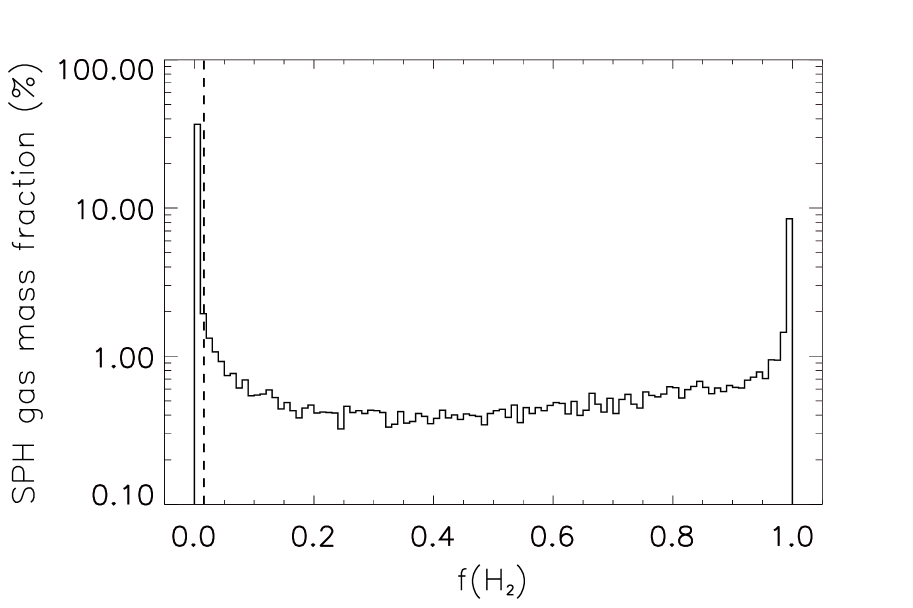
Following the above prescription sígame determines the molecular gas mass fraction and thus the molecular gas mass ($m_{\rm mol}=\mbox{$f^{\prime}_{\rm mol}$}m_{\rm SPH}$) associated with each SPH particle. Depending on the environment (e.g., $G_{0}^{\prime}$, $Z^{\prime}$, $T_{\rm{k}}$, $P_{\rm{ext}}$,…), the fraction of the SPH gas converted into H₂ can take on any value between 0 and 1, as seen from the $f^{\prime}_{\rm mol}$ distribution of G1 in Figure 4. Overall, the total mass fraction of the SPH gas in G1, G2, and G3 (i.e., within $R_{\rm cut}$) that is converted to molecular gas is $29$ %, $52$ % and $34$ %, respectively.

Figure 4: The distribution of the H₂ gas mass fraction of the SPH particles in G1 calculated according to eq. 3 (solid line histogram). Similar distributions are found for G2 and G3. The lower limit on $f^{\prime}_{\rm mol}$, defined as described in Section 3.4.1, is indicated by the dashed vertical line.

3.4 Structure of the molecular gas

Having determined the molecular gas mass fractions, sígame proceeds by distributing the molecular gas into GMCs, and calculates their masses and sizes, along with internal density and temperature structures, as described in the following.

3.4.1 GMC masses and sizes

The molecular gas associated with a given SPH particle is divided into GMCs by randomly sampling a power-law mass spectrum of the form:

$$\frac{dN}{dm_{\rm GMC}}\propto\mbox{$m_{\rm{GMC}}$}^{-\beta}.$$ (8)

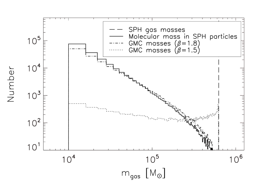
For GMCs in the MW disk and Local Group galaxies $\beta\simeq 1.8$ (Blitz et al., 2007), and is the value adopted by sígame in this paper unless otherwise stated. Lower and upper mass cut-offs at $10^{4}\,\mbox{$\rm{M}_{\odot}$}$ and $10^{6}\,\mbox{$\rm{M}_{\odot}$}$, respectively, are enforced in order to span the mass range observed by Blitz et al. (2007). A similar approach was adopted by Narayanan et al. (2008b); Narayanan et al. (2008c). Note that, in the case of G1 the upper cut-off on the GMC masses is in fact set by the mass resolution of the SPH simulation ($6.3\times 10^{5}\,h^{-1}\,{\rm\mbox{$\rm{M}_{\odot}$}}$). For G1, typically $\lesssim 30$ GMCs are created in this way per SPH particle, while for G2 and G3, which were run with SPH gas particle masses almost an order of magnitude higher, as much as $\sim 100$ GMCs could be extracted from a given SPH particle. Figure 5 shows the resulting mass distribution of all the GMCs in G1, along with the distribution of molecular gas mass associated with the SPH gas particles prior to it being divided into GMCs. The net effect of re-distributing the H₂ mass into GMCs is a mass distribution dominated by relatively low cloud masses, which is in contrast to the relatively flat SPH H₂ mass distribution. Note, the lower cut-off at $\mbox{$m_{\rm{GMC}}$}=10^{4}\,\mbox{$\rm{M}_{\odot}$}$ implies that if the molecular gas mass associated with an SPH particle (i.e., $m_{\rm mol}=\mbox{$f^{\prime}_{\rm mol}$}m_{\rm SPH}$) is less than this lower limit it will not be re-distributed into GMCs. Since $m_{\rm SPH}$ is constant in our simulations ($6.3\times 10^{5}\,h^{-1}\,\mbox{$\rm{M}_{\odot}$}$ for G1 and $4.7\times 10^{6}\,h^{-1}\,\mbox{$\rm{M}_{\odot}$}$ for G2 and G3) the lower limit imposed on $m_{\rm GMC}$ translates directly into a lower limit on $f^{\prime}_{\rm mol}$ ($0.016$ for G1 and 0.002 for G2 and G3, shown as a dashed vertical line for G1 in Figure 4). As a consequence, 0.2, 0.005 and 0.01 % of the molecular gas in G1, G2, and G3, respectively, does not end up in GMCs. These are negligible fractions and the molecular gas they represent can therefore be safely ignored.

Figure 5: The distribution of GMC masses in G1 obtained by applying eq. 8, with $\beta=1.8$ (solid histogram) and $\beta=1.5$ (dash-dotted histogram), compared to the total molecular gas masses associated with SPH particles (distribution shown as dotted histogram). The dashed vertical line indicates the SPH gas mass resolution of the simulation ($=6.3\times 10^{5}\,h^{-1}\,{\rm\mbox{$\rm{M}_{\odot}$}}$ in the case of G1).

The GMC sizes are derived from the virial theorem, which relates the radius of a GMC ($R_{\rm{GMC}}$) to its mass and external pressure ($P_{\rm{ext}}$) according to:

$$\frac{\mbox{$R_{\rm{GMC}}$}}{\text{pc}}=\left(\frac{\mbox{$P_{\rm{ext}}$}/k_{\rm B}}{10^{4}\,\mbox{cm${}^{-3}$}\,{\rm K}}\right)^{-1/4}\left(\frac{\mbox{$m_{\rm{GMC}}$}}{290\,\mbox{$\rm{M}_{\odot}$}}\right)^{1/2}.$$ (9)

Similarly, the internal velocity dispersion ($\sigma_{v}$) of the clouds is given by:

$$\frac{\sigma_{v}}{{\rm km\,s^{-1}}}=1.2\left(\frac{\mbox{$P_{\rm{ext}}$}/k_{\rm B}}{10^{4}\,\mbox{cm${}^{-3}$}\,{\rm K}}\right)^{1/4}\left(\frac{\mbox{$R_{\rm{GMC}}$}}{\rm{pc}}\right)^{1/2}$$ (10)

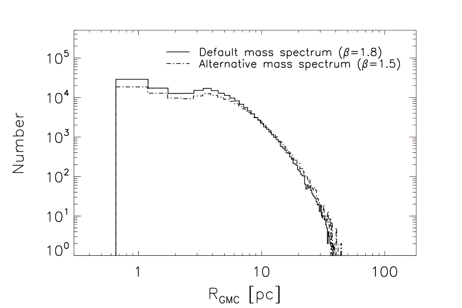
(e.g., Elmegreen, 1989; Swinbank et al., 2011). Figure 6 shows the resulting distribution of GMC radii in G1 (solid histogram). The minimum and maximal cloud radii found in G1 are $\sim 0.07\,{\rm pc}$ and $\sim 100\,{\rm pc}$, respectively, and are set by the pressure and the imposed limits on $m_{\rm GMC}$.

Observations have indicated that the shape of the GMC mass spectrum might be different in gas-rich systems where a high-pressure ISM leads to the characteristic mass of star-forming clumps of molecular gas being much higher than what is observed in normal spirals (e.g. Swinbank et al., 2011; Leroy et al., 2015). In Section 5 we therefore examine the effects of adopting a more top-heavy GMC mass distribution, corresponding to $\beta=1.5$ (shown as dot-dashed histogram in Figure 5). The total amount of molecular gas in our galaxies does not change significantly between $\beta=1.8$ and $\beta=1.5$, and the CO simulation results are robust against (reasonable) changes in the mass-spectrum.

The GMCs are placed randomly around the position of their ‘parent’ SPH particle, albeit with an inverse proportionality between radial displacement and mass of the GMC. The latter is done in order to retain the mass distribution of the original galaxy simulation as best as possible. The GMCs are assigned the same bulk velocity, $\bar{v}$, $Z^{\prime}$, $G_{0}^{\prime}$ and $\zeta_{\rm{CR}}$ as their ‘parent’ SPH particle.

Figure 6: The distribution of GMC radii in G1 for the adopted cloud mass spectrum with $\beta=1.8$ (solid histogram) and for a slightly modified spectrum with $\beta=1.5$ (dash-dotted histogram). Similar distributions are found for G2 and G3.

3.4.2 GMC density structure

In order to ensure a finite central density in our GMCs, sígame adopts a Plummer radial density profile (e.g., Plummer, 1911; Whitworth & Ward-Thompson, 2001):

$$\frac{n_{\text{H}_{2}}(R)}{\mbox{cm${}^{-3}$}}=3.55\left(\frac{m_{\rm GMC}}{\mbox{$\rm{M}_{\odot}$}}\right)\left(\frac{R_{p}}{{\rm pc}}\right)^{-3}\left(1+\frac{R^{2}}{R_{p}^{2}}\right)^{-5/2},$$ (11)

where $R_{p}$ is the so-called Plummer radius, which we set to $R_{p}=0.1\mbox{$R_{\rm{GMC}}$}$. The latter allows for a broad range in gas densities throughout the clouds, from $\sim 10^{5}$ cm^-3 in the central parts to a few $10\,\mbox{cm${}^{-3}$}$ further out. Note, eq. 11 accounts for the presence of helium in the GMC.

In Section 5 we examine the impact on our simulation results if a steeper GMC density profile with an exponent of $-7/2$ is adopted instead of the default $-5/2$ in eq. 11. This modified Plummer profile, as well as the default profile, are shown in Figure 7 for a GMC with mass of $10^{4}$ $\rm{M}_{\odot}$ and external pressure $10^{4}\,{\rm K\,cm^{-3}}$.

Figure 7: Plummer density profiles (eq. 11) with exponents $-5/2$ (solid line) and $-7/2$ (dashed line) for a GMC mass of $10^{4}$ $\rm{M}_{\odot}$ and an external pressure of $\mbox{$P_{\rm{ext}}$}/k_{\rm B}=10^{4}\,$K cm^-3. The corresponding cloud radius is $\mbox{$R_{\rm{GMC}}$}=5.9$ pc (eq. 9). The vertical dash-dotted line marks the Plummer radius ($=0.1R_{\rm GMC}$), and the horizontal dotted line the $n_{\rm{H}_{2}}$ value ($50\,{\rm cm^{-3}}$) below which CO is assumed to photo-dissociate in our simulations.

3.4.3 GMC thermal structure

Having established the masses, sizes, and density structure of the GMCs, sígame solves for the kinetic temperature throughout the clouds by balancing the relevant heating and cooling mechanisms as a function of cloud radius.

GMCs are predominantly heated by FUV photons (via the photo-electric effect) and cosmic rays. For the strength of the FUV field impinging on the GMCs, we take the previously calculated values at the SPH gas particle position (eq. 2). We shall assume that the CR ionization rate scales in a similar manner, since CRs have their origin in supernovae and are therefore related to the star formation and the total stellar mass of the galaxy:

$$\zeta_{\rm{CR}} =\zeta_{\rm CR,MW}\left(0.5\frac{{\rm SFRD}_{\rm{local}}}{{\rm SFRD}_{\rm{MW}}}+0.5\frac{{\rm M}_{*}}{{\rm M}_{\rm*,MW}}\right)$$ (12)

where ${\rm SFRD}_{\rm{local}}$, ${\rm SFRD}_{\rm{MW}}$ and ${\rm M}_{\rm*,MW}$ are as described in Section 3.3, and $\zeta_{\rm{CR}}$ is scaled to the ‘canonical’ MW value of $\zeta_{\rm{CR}}$ ${}_{\rm,MW}=3\times 10^{-17}$ s^-1 (e.g. Webber, 1998). While the FUV radiation is attenuated by dust and therefore does not heat the GMC centres significantly, cosmic rays can penetrate these dense regions and heat the gas there (Papadopoulos et al., 2011). For this reason sígame attenuates the FUV field throughout the GMCs, while the CR ionization rate remains constant for a given cloud. The extinction of the FUV field at a certain point within a GMC is derived by integrating the Plummer density profile from that point and out to $R_{\rm{GMC}}$. This H column density is converted into a visual extinction ($A_{\rm V}=\mbox{$N_{\rm{H}}$}/2.2\times 10^{21}\,\mbox{cm${}^{-2}$}$) so that the attenuated FUV field becomes:

$$\mbox{$G_{0{\rm,att}}^{\prime}$}=\mbox{$G_{0}^{\prime}$}e^{-1.8A_{\rm V}},$$ (13)

where the factor of $1.8$ is the adopted conversion from visual to FUV extinction (Black & Dalgarno, 1977).

sígame calculates the gas kinetic temperature throughout each GMC via the following heating and cooling rate balance:

$$\mbox{$\Gamma_{\rm{PE}}$}+\mbox{$\Gamma_{\rm{CR,H}_{2}}$}=\mbox{$\Lambda_{\rm{H}_{2}}$}+\mbox{$\Lambda_{\rm{CO}}$}+\mbox{$\Lambda_{\rm{O}\rm{\textsc{i}}}$}+\mbox{$\Lambda_{\rm{C}\rm{\textsc{ii}}}$}+\mbox{$\Lambda_{\rm{gas-dust}}$}.$$ (14)

$\Gamma_{\rm{PE}}$ is the photo-electric heating by FUV photons, and $\Gamma_{\rm{CR,H}_{2}}$ is the cosmic ray heating in molecular gas. $\Lambda_{\rm{H}_{2}}$ is the cooling rate of the two lowest H₂ rotational lines (S(0) and S(1)), and $\Lambda_{\rm{CO}}$ is the cooling rate of the combined CO rotational ladder. $\Lambda_{\rm{gas-dust}}$ is the cooling rate due to interactions between gas molecules and dust particles, which only becomes important at densities above $10^{4}$ cm^-3 (e.g., Goldsmith, 2001; Glover & Clark, 2012). $\Lambda_{\rm{C}\rm{\textsc{ii}}}$ and $\Lambda_{\rm{O}\rm{\textsc{i}}}$ are the cooling rates due to [Cii] and [Oi] line emission, respectively. The abundances of carbon and oxygen used in the prescriptions for their cooling rates, scale with the cloud metallicity, while the CO cooling scales with the relative CO to neutral carbon abundance ratio, set by the molecular density (see Appendix B).

$\Lambda_{\rm{gas-dust}}$ depends on the temperature difference between the gas and the dust (see eq. 29). The dust temperature, $T_{\rm{dust}}$, is set by the equilibrium between the absorption of FUV and the emission of IR radiation by the dust grains. We adopt the approximation given by Tielens (2005):

$$\frac{\mbox{$T_{\rm{dust}}$}}{{\rm K}}\simeq 33.5\left(\frac{a}{1\mu{\rm m}}\right)^{-0.2}\left(\frac{\mbox{$G_{0{\rm,att}}^{\prime}$}}{10^{4}\,{\rm Habing}}\right)^{0.2},$$ (15)

where $G_{0{\rm,att}}^{\prime}$ is the dust-attenuated FUV field (eq. 13) and $a$ is the grain size, which we set to 1 $\mu$m for simplicity. Values for $T_{\rm{dust}}$ using eq. 15 range from 0 to 8.9 K, but we enforce a lower limit on $T_{\rm{dust}}$ equal to the $z=2$ CMB temperature of $8.175$ K. $T_{\rm{dust}}$ is therefore essentially constant ($\sim 8-9$ K) throughout the inner region of the GMC models, similar to the value of $\mbox{$T_{\rm{dust}}$}=8$ K adopted by Papadopoulos & Thi (2013) for CR-dominated cores. Analytical expressions for all of the above heating and cooling rates are given in Appendix B, which also shows their relative strengths as a function of density for two example GMCs (Figure 14).

Figure 16 in Appendix C shows the resulting $T_{\rm{k}}$ versus $n_{\rm{H}_{2}}$ behaviour for 80 GMCs spanning a broad range of GMC masses, metallicities, and star formation rate densities. As seen in the displayed GMC models, some general trends can be inferred from the $\mbox{$T_{\rm{k}}$}-\mbox{$n_{\rm{H}_{2}}$}$ diagrams. At fixed metallicity and mass, an increase in $G_{0}^{\prime}$ (and therefore also in $\zeta_{\rm{CR}}$), leads to higher temperatures throughout the models. In the outer regions this is due primarily to the increased photoelectric heating, while in the inner regions, heating by the unattenuated cosmic rays takes over as the dominating heating mechanism (Figure 14). Keeping $G_{0}^{\prime}$ (and $\zeta_{\rm{CR}}$) fixed, lower $T_{\rm{k}}$-levels and shallower $\mbox{$T_{\rm{k}}$}-\mbox{$n_{\rm{H}_{2}}$}$ gradients are found in GMCs with higher metallicities. Both these trends are explained by the fact that the [Cii] and [Oi] cooling rates scale linearly with $Z^{\prime}$ (see Appendix B).

Moving from the outskirts and inward towards the GMC centres, $T_{\rm{k}}$ drops as the attenuation of $G_{0}^{\prime}$ reduces the photoelectric heating. However, the transition from cooling via [Cii] to the less efficient cooling mechanism by CO lines, causes a local increase in $T_{\rm{k}}$ at $\mbox{$n_{\rm{H}_{2}}$}\sim 10^{3}-10^{4.5}$ cm^-3, as also seen in the detailed GMC simulations by Glover & Clark (2012). The exact density at which this ‘bump’ in $T_{\rm{k}}$ occurs depends strongly on the mass of the GMC. Our choice of the Plummer model for the radial density profile means that the extinction, $A_{\rm V}$, at a certain density increases with GMC mass. This in turn decreases the FUV heating, and as a result the $\mbox{$T_{\rm{k}}$}-\mbox{$n_{\rm{H}_{2}}$}$ curve moves to lower densities with increasing GMC mass.

As the density increases towards the cloud centres (i.e., $n_{\rm H_{2}}\gtrsim 10^{4-5}$ cm^-3) molecular line cooling and also gas-dust interactions become increasingly efficient and start to dominate the cooling budget. The $\mbox{$T_{\rm{k}}$}-\mbox{$n_{\rm{H}_{2}}$}$ curves are seen to be insensitive to changes in $Z^{\prime}$, which is expected since the dominant heating and cooling mechanisms in these regions do not depend on $Z^{\prime}$. Eventually, in the very central regions of the clouds, the gas reaches temperatures close to that of the ambient CMB radiation field, irrespective of the overall GMC properties and the conditions at the surface (Figure 14).

3.4.4 GMC grid models

The $\mbox{$T_{\rm{k}}$}-\mbox{$n_{\rm{H}_{2}}$}$ curve for a given GMC is determined by the following quantities:

• $G_{0}^{\prime}$ and $\zeta_{\rm{CR}}$, which govern the gas heating and are set by the local star formation rate density (SFRD_local) and the total stellar mass ($M_{*}$) according to eqs. 2 and 12.

• $m_{\rm{GMC}}$ and $P_{\rm{ext}}$ which determine the effective radius of a cloud (eq. 9) and thus its density profile (eq. 11).

• The local metallicity ($Z^{\prime}$), which influences the fraction of H₂ gas and plays an important role in cooling the gas.

These local parameters together with the most important global parameters used by sígame are listed in Table 2. The GMC ensemble distributions of $G_{0}^{\prime}$, $\zeta_{\rm{CR}}$, $m_{\rm{GMC}}$, $\mbox{$P_{\rm{ext}}$}/k_{\rm B}$, and $Z^{\prime}$ for each of the galaxies G1, G2 and G3 are shown in Figure 15.

There are more than $100,000$ GMCs in a single model galaxy and, as Figure 15 shows, they span a wide range in $G_{0}^{\prime}$, $\zeta_{\rm{CR}}$, $m_{\rm{GMC}}$, $\mbox{$P_{\rm{ext}}$}/k_{\rm B}$, and $Z^{\prime}$. Thus, in order to shorten the computing time, we calculated $\mbox{$T_{\rm{k}}$}-\mbox{$n_{\rm{H}_{2}}$}$ curves for a set of 630 GMCs, chosen to appropriately sample the distributions at certain grid values (listed in Table 3, and marked by vertical black lines in Figure 15). Every GMC in our simulations was subsequently assigned the $\mbox{$T_{\rm{k}}$}-\mbox{$n_{\rm{H}_{2}}$}$ curve of the GMC grid model closest to it in the ($G_{0}^{\prime}$, $m_{\rm GMC}$, $Z^{\prime}$) parameter space. In the default GMC grid, we keep $\mbox{$P_{\rm{ext}}$}/k_{\rm B}$ fixed to a MW-like value of $10^{4}\,\rm{K}\,\mbox{cm${}^{-3}$}$, thereby also anchoring the scaling relations in eq. 9 and 10 for size and velocity dispersion. This is done to minimise the number of radiative transfer calculations, effectively keeping the amount of molecular gas mass dependent on local pressure, but removing local pressure as a free parameter in, and hence simplifying, the calculation of CO emission.

In addition to the default grid described above, we made two separate tests to explore the GMC parameter space more fully. These tests are described in the following and results of their application are presented in Section 5. The external cloud pressure, $\mbox{$P_{\rm{ext}}$}/k_{\rm B}$, spans a wide range from $\sim 10^{3}$ to $10^{9}\,\rm{K}\,\mbox{cm${}^{-3}$}$ as shown in Figure 15. In a separate test, we therefore constructed the same GMC grid, but for fixed pressures of $\mbox{$P_{\rm{ext}}$}/k_{\rm B}=10^{5.5}\,$ and $10^{6.5}\,$K cm^-3 and interpolated among the resulting three values of $\mbox{$P_{\rm{ext}}$}/k_{\rm B}$ ($[10^{4},10^{5.5},10^{6.5}]\,$K cm^-3) as a demonstration of how to incorporate local pressure in sígame. We also test the effect of adopting the alternative radial GMC density profile defined in Section 3.4.2. $\mbox{$T_{\rm{k}}$}-\mbox{$n_{\rm{H}_{2}}$}$ curves were calculated for each possible combination of the parameter grid values listed in Table 3 for both density profiles, giving us a total of $3\times 2\times 630=3780$ GMC grid models.

Table 2: Parameters, global and local, used by sígame, together with relevant equations in this paper.

Global parameters	[CO/H2 ], $\beta$ (GMC mass spectrum), GMC density profile	Eqs. 8 and 11
Local parameters	$m_{\rm{GMC}}$, $G_{0}^{\prime}$, $\zeta_{\rm{CR}}$, $Z^{\prime}$, $P_{\rm{ext}}$, SFRD	Eqs. 8, 2, 2 and 6
Derived internal GMC parameters	$n_{\rm{H}}$, $T_{\rm{k}}$, $x_{\rm{e}}$, $\sigma_{\rm{v}}$	Eqs. 11 and 14

Table 3: Grid parameter values

$G_{0}^{\prime}$ [Habing]	0.5, 1, 4, 7, 10, 13, 16, 19, 23, 27
$\log(\mbox{$m_{\rm{GMC}}$}\,[\mbox{$\rm{M}_{\odot}$}])$	4.0, 4.25, 4.5, 4.75, 5.0, 5.25, 5.5, 5.75, 6.0
$\log(Z/Z_{\odot})$	-1, -0.5, 0, 0.5, 1, 1.4, 1.8
$\log(\mbox{$P_{\rm{ext}}$}/k_{\rm B}\,{\rm[K\,\mbox{cm${}^{-3}$}]})$	4.0, 5.5, 6.5

3.5 Radiative transfer of CO lines

sígame assumes a fixed CO abundance equal to the Galactic value of [CO/H₂ ]$=2\times 10^{-4}$ (Lee et al., 1996; Sofia et al., 2004, and see Section 6 for a justification of this value) everywhere in the GMCs except for $\mbox{$n_{\rm{H}_{2}}$}<50$ cm^-3, where CO is not expected to survive photo-dissociation processes (e.g. Narayanan et al., 2008c). sígame calculates the CO line radiative transfer for each GMC individually and derives the CO line emission from the entire galaxy.

3.5.1 Individual GMCs

For the CO radiative transfer calculations we use a slightly modified version of the LIne Modeling Engine (lime ver. 1.4; Brinch & Hogerheijde, 2010) - a 3D molecular excitation and radiative transfer code. lime has been modified in order to take into account the redshift dependence of the CMB temperature, which is used as boundary condition for the radiation field during photon transport, and we have also introduced a redshift correction in the calculation of physical sizes as a function of distance. We use collision rates for CO (assuming H₂ is the main collision partner) from Yang et al. (2010). In lime, photons are propagated along grid lines defined by Delaunay triangulation around a set of appropriately chosen sample points in the gas, each of which contain information on $n_{\rm{H}_{2}}$, $T_{k}$, $\sigma_{v}$, $[{\rm CO}/\mbox{{\sc H}${}_{2}$}]$ and $\boldsymbol{v}$. sígame constructs such a set of sample points throughout each GMC: about 5000 points distributed randomly out to a radius of $50$ pc, i.e., beyond the effective radius of typical GMCs in G1, G2, and G3 (Figure 6) and in a density regime below the threshold density of $50$ cm^-3 adopted for CO survival (see previous paragraph). The concentration of sample points is set to increase towards the centre of each GMC where the density and temperature vary more drastically.

For each GMC, lime generates a CO line data cube, i.e., a series of CO intensity maps as a function of velocity. The velocity-axis consists of 50 channels, each with a spectral resolution of $1.0$ km s^-1, thus covering the velocity range $v=[-25,+25]\,{\rm km\,s^{-1}}$. The maps are $100\,{\rm pc}$ on a side and split into 200 pixels, corresponding to a linear resolution of $0.5\text{\,pc/pixel}$ (or an angular resolution of $5.9\times 10^{-5}\,\arcsec\text{/pixel}$ at $z=2$). Intensities are corrected for arrival time delay and redshifting of photons.

Figure 17 shows the area- and velocity-integrated CO Spectral Line Energy Distributions (SLEDs) for the same 80 GMCs used in Section 3.4.3 to highlight the $\mbox{$T_{\rm{k}}$}-\mbox{$n_{\rm{H}_{2}}$}$ profiles (Figure 16). The first thing to note is that the CO line fluxes increase with $m_{\rm{GMC}}$, which is due to the increase in size, i.e., surface area of the emitting gas, with cloud mass (Section 3.4.1). Turning to the shape of the CO SLEDs, a stronger $G_{0}^{\prime}$ (and $\zeta_{\rm{CR}}$) increases the gas temperature and thus drives the SLEDs to peak at higher $J$-transitions. Only the higher, $J_{\rm up}>4$, transitions are also affected by metallicity, displaying increased flux with increased $Z^{\prime}$. For GMCs with high $G_{0}^{\prime}$, the high metallicity levels thus cause the CO SLED to peak at $J_{\rm up}>8$.

3.5.2 The effects of dust

Dust absorbs the UV light from young O and B stars and re-emits in the far-IR, leading to possible ‘IR pumping’ of molecular infrared sources. However, due to the large vibrational level spacing of CO, the molecular gas has to be at a temperature of at least $159$ K, for significant IR pumping of the CO rotational lines to take place, when assuming a maximum filling factor of 1, as shown by Carroll & Goldsmith (1981). Most of the gas in our GMC models is at temperatures below $100$ K, with only a small fraction of the gas, in the very outskirts, of the GMCs reaching $\mbox{$T_{\rm{k}}$}>159$ K, as seen in Figure 16 in Appendix C. This happens only if the metallicity is low ($\mbox{$Z^{\prime}$}\leq 0.1$) or in case of a combination between high FUV field ($\mbox{$G_{0}^{\prime}$}\geq 4$) and moderate metallicity.

In principle, the high-$J$ CO lines could be subject to extinction by dust, but this effect is significant only in extremely dust-enshrouded sources (Papadopoulos et al., 2010), and therefore unlikely to be relevant for our simulations.

While lime is capable of including dust in the radiative transfer calculations, provided that a table of dust opacities as function of wavelength be supplied together with the input model, we have chosen not to include dust in the simulations presented here.

Figure 8: Top row: Molecular surface density maps of our model galaxies seen face-on. The maps have been smoothed using a circular Gaussian with full width at half maximum (FWHM) of $3$ pixels corresponding to $0.24$ kpc. The molecular gas surface density maps are seen to trace the spiral arms and inner disk as well as a few dense clumps further out. Bottom row: azimuthally averaged radial profiles of the molecular (solid curve) and Hi +Hii (dashed curve) gas surface densities, of the mean metallicity (dotted curve) and of $G_{0}^{\prime}$ (dot-dashed curve) – determined from 50 radial bins stretching from 0 to 15 kpc from the centre of each galaxy. The molecular gas is the result of applying the recipes in Section 3.3 to the SPH simulations presented in Section 2.2, while the $\mbox{{\rm{H}{i}}}+\mbox{\rm{H}{ii}}$ gas is the initial SPH gas mass minus the derived molecular gas mass (both include the contribution from helium). We estimate $G_{0}^{\prime}$ by averaging over the FUV fields impinging on all GMCs in each radial bin.

3.5.3 CO emission maps

A given GMC is assigned the CO emission line profile of the GMC model that corresponds to the nearest grid point in the ($G_{0}^{\prime}$, $m_{\rm{GMC}}$, $Z^{\prime}$) parameter space. A spatial grid of $400\times 400$ pixels is overlayed on each galaxy viewed face-on, and the line profiles of all GMCs within each pixel are added to a common velocity axis, thus resulting in a position-velocity datacube. CO moment 0 maps are then constructed by integrating the flux within each pixel in velocity. These maps are $40\,{\rm kpc}$ on each side and thus have a resolution of $\sim 100\,{\rm pc/pixel}$. By expanding the pixel size to encompass the entire galaxy, the global CO SLED is derived.

The approach described above assumes that the molecular line emission from each GMC is radiatively decoupled from all other GMCs, due to the significant velocity gradients across the galaxies ($\sim 200-500$ km s^-1) and the relatively small internal line widths of the individual GMCs ($\sim 2-34$ km s^-1 for the GMCs in G1, G2 and G3).

Figure 9: The top three rows show the moment 0 maps of the CO(1$-$0), CO(3$-$2) and CO(7$-$6) emission from G1, G2 and G3. The CO maps have been smoothed using a circular Gaussian with full width at half maximum (FWHM) of 3 pixels corresponding to $0.24$ kpc, and as with the SPH and molecular gas surface density maps, a logarithmic scale has been applied in order to better display extended emission. The bottom row shows the azimuthally averaged CO 3$-$2/1$-$0 and 7$-$6/1$-$0 brightness temperature line ratios (denoted $r_{32}$ and $r_{76}$, respectively) as functions of projected radius for each of the three galaxies. A radial bin-size of $0.5\,{\rm kpc}$ was used. Also shown are the azimuthally averaged radial profiles of CO-to-H₂ conversion factor $\alpha_{\rm CO}(R)=\Sigma_{\mbox{{\sc H}${}_{2}$}}/I_{{\rm CO}(1-0)}$ in units of $\rm{M}_{\odot}$  pc^-2 (K km s^-1)^-1 with a dashed line indicating the global $\alpha_{\rm CO}$ factor and a dotted line for the disk-averaged $\alpha_{\rm CO}$ factor (see Section 4.2).

4 Simulating massive $z=2$ main sequence galaxies

In this section we examine the H₂ surface density and CO emission maps resulting from applying sígame to the three SPH galaxy simulations G1, G2, and G3 at $z=2$ (Section 2), and we compare with existing CO observations of main sequence galaxies at $z\sim 1-2.5$. We also tested sígame on three MW-like galaxies (see Appendix D), finding a general agreement with the CO line observations of MW and other similar local galaxies. As mentioned in previous sections, our default grid will be that corresponding to a Plummer density profile and a pressure of $\mbox{$P_{\rm{ext}}$}/k_{\rm B}=10^{4}\,{\rm\mbox{cm${}^{-3}$}\,K}$, combined with a GMC mass spectrum of slope $\beta=1.8$, unless otherwise stated.

4.1 Total molecular gas content and H₂ surface density maps

The total molecular gas masses of G1, G2 and G3 – obtained by summing up the GMC masses associated with all SPH particles within each galaxy (i.e., $M_{\rm mol}=\sum\mbox{$m_{\rm{GMC}}$}=\sum\mbox{$f^{\prime}_{\rm mol}$}m_{\rm SPH}$) – are $7.1\times 10^{9}$, $1.7\times 10^{10}$, and $2.1\times 10^{10}$ $\rm{M}_{\odot}$, respectively, corresponding to about $34$, $59$ and $45$ % of the original total SPH gas masses of the galaxies within $R_{\rm cut}=20\,$kpc. The global molecular gas mass fractions (i.e., $f_{\rm mol}=M_{\rm mol}/(M_{*}+M_{\rm mol}$) are 11.8, 10.2 and 9.1 % for G1, G2, and G3, respectively.

This is $\sim 4-5\times$ below the typical molecular gas mass fraction ($\sim 40-60\,\%$) inferred from CO observations of main sequence galaxies at $z\sim 1-3$ with similar stellar masses and star formation rates as our simulations (e.g., Daddi et al., 2010; Magnelli et al., 2012; Tacconi et al., 2013).

The reason for this discrepancy is the low SPH gas mass fractions of our simulated galaxies to begin with ($f_{\rm SPH}=M_{\rm SPH}/(M_{*}+M_{\rm SPH})=18-28$ %), which obviously restricts $f_{\rm mol}$ to lower values. Such low gas fractions have been observed in local star forming galaxies. For example, assuming a MW-like $\alpha_{\rm CO}$ factor, Saintonge et al. (2011) derived $f_{\rm mol}\sim 6.7\pm 4.5$ % for a sample of 119 CO$(1-0)$ detected normal star forming galaxies and a stack of 103 non-detections.

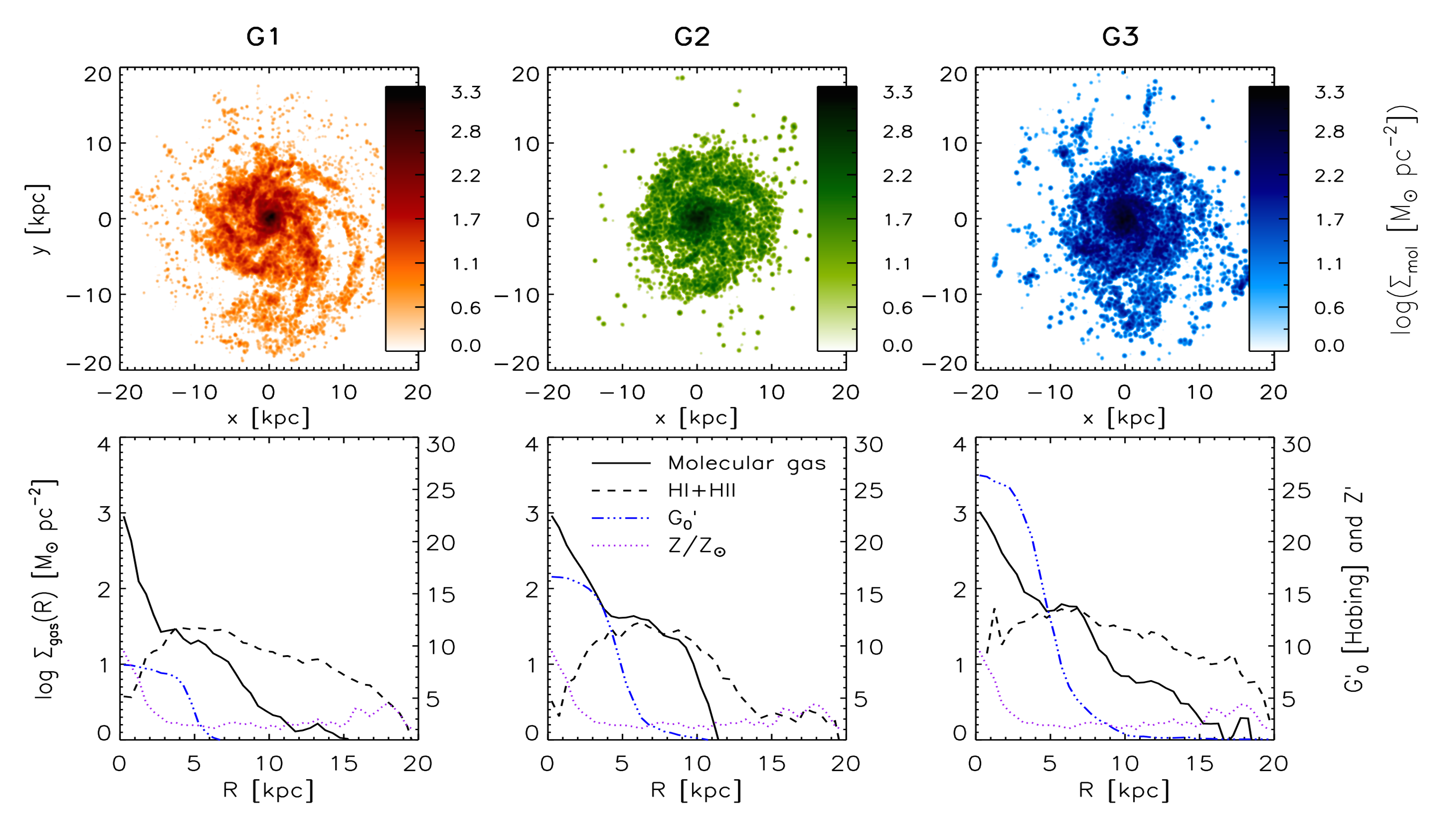
Figure 8 (top panels) shows the molecular gas surface density ($\Sigma_{\rm{mol}}$) maps of G1, G2, and G3, where $\Sigma_{\rm{mol}}$ is calculated over pixels $80\,{\rm pc}\times 80\,{\rm pc}$ in size. The pixel size was chosen in order to avoid resolving the GMCs, which typically have sizes $\mathrel{\raise 1.50696pt\hbox{$\scriptstyle<$}\kern-6.00006pt\lower 1.72218pt\hbox{{$\scriptstyle\sim$}}}40\,{\rm pc}$ (see Figure 6). The molecular gas is seen to extend out to radii of $\sim 10\,{\rm kpc}$ and beyond, but generally the molecular gas concentrates within the inner regions of each galaxy. The distribution of molecular gas broadly follows the central disk and spiral arms where the SPH surface density ($\Sigma_{\rm SPH}$) is also the highest (Figure 1). The correspondence is far from one-to-one, however, as seen by the much larger extent of the SPH gas, i.e., regions where H₂ has not formed despite the presence of atomic and ionised gas. This point is further corroborated in the bottom panels of Figure 8, which show azimuthally-averaged radial surface density profiles of the molecular gas and of the $\mbox{{\rm{H}{i}}}+\mbox{\rm{H}{ii}}$ gas. The latter is simply the initial SPH gas mass with the molecular gas mass subtracted, and has been corrected (just like the molecular gas phase) for the mass contribution from helium.

In order to compare $\Sigma_{\rm H{\sc I}+H{\sc II}}$ and $\Sigma_{\rm{mol}}$ with observations, we have set the radial bin width to $0.5$ kpc – the typical radial bin size used for nearby spirals in the work of Leroy et al. (2008). The radially binned $\Sigma_{\rm{mol}}$ reaches $\sim 800-1000$ $\rm{M}_{\odot}$  pc^-2 in the central regions of our simulated galaxies, which is comparable to observational estimates of $\Sigma_{\rm{mol}}$ (of several 100 $\rm{M}_{\odot}$  pc^-2) towards the centres of nearby spirals (Leroy et al., 2008). In all three galaxies, the Hi+Hii surface density dips within the central $\sim 1-2\,{\rm kpc}$, coinciding with a strong peak in $\Sigma_{\rm{mol}}$. Thus, despite the marked increase in the FUV radiation field towards the centre, the formation of H₂ driven by the increase in gas pressure is able to overcome photodestruction of H₂ through absoption of Lyman or Werner band radiation. The central H₂ surface densities are similar for all galaxies and is a direct consequence of very similar SPH gas surface densities in the centre combined with molecular gas mass fractions approaching 1. From $R\sim 2\,{\rm kpc}$ and out to $\sim 10\,{\rm kpc}$, the $\mbox{{\rm{H}{i}}}+\mbox{\rm{H}{ii}}$ surface density remains roughly constant with values of $\sim 40$, $\sim 70$ and $\sim 100$ $\rm{M}_{\odot}$  pc^-2 for G1, G2 and G3, respectively.

Radial profiles of the Hi and molecular gas surface density that are qualitatively very similar to our simulations have been observed in several nearby star-forming disk galaxies (e.g., Leroy et al., 2008; Bigiel et al., 2008). In local galaxies, however, the Hi surface density, including helium, rarely exceeds $\sim 10$ $\rm{M}_{\odot}$  pc^-2, while in our simulations we find Hi +Hii surface densities that are $4-10\times$higher, which is due to the substantial fraction of ionised gas in our simulated galaxies.

4.2 CO line emission maps and resolved excitation conditions

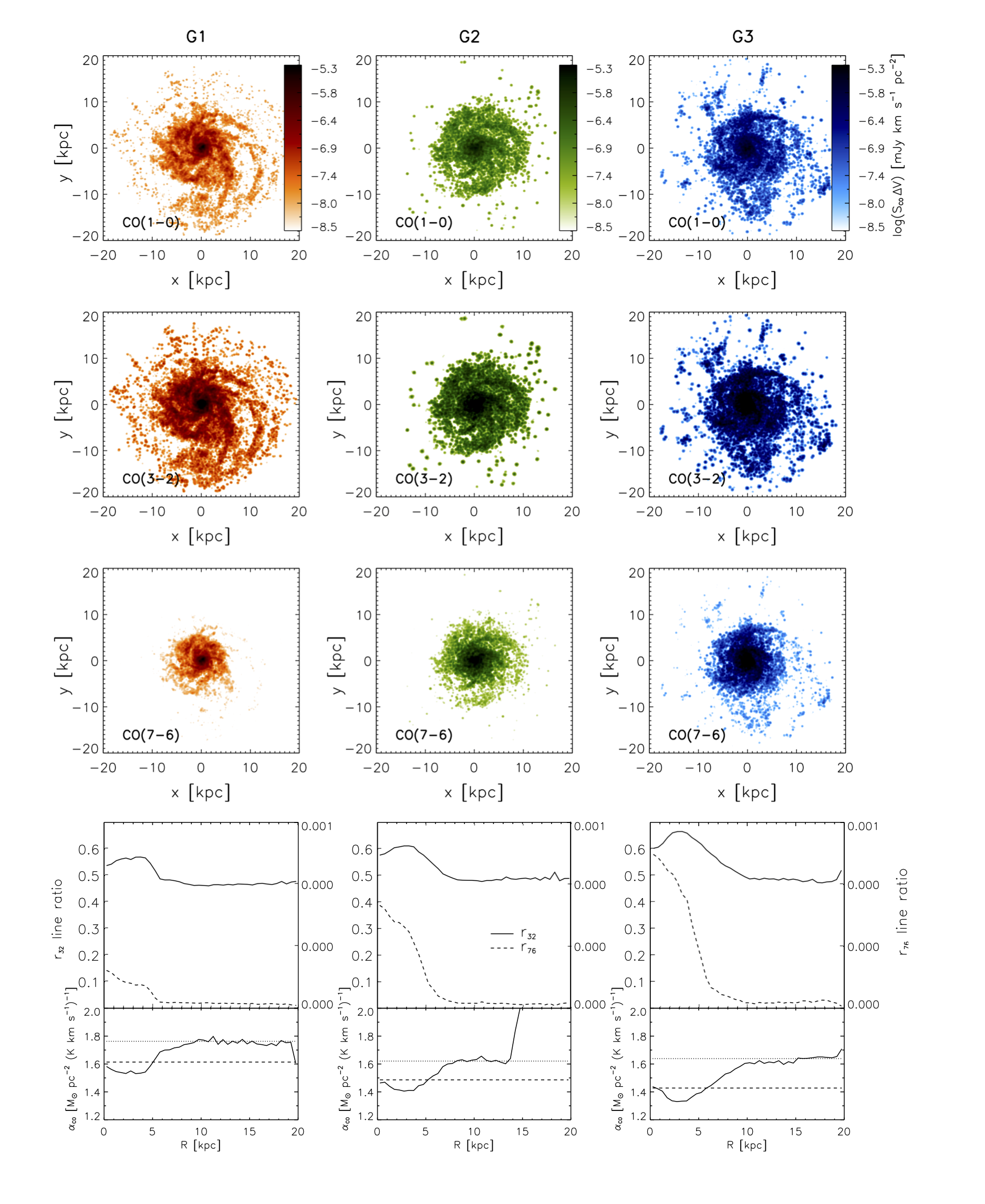
Moment 0 maps of the CO(1$-$0), CO(3$-$2) and CO(7$-$6) emission from G1, G2 and G3 are shown in Figure 9. Both the CO(1$-$0) and CO(3$-$2) emission are seen to trace the H₂ gas distribution well (Figure 8), while the CO(7$-$6) emission only trace gas in the central $\sim 7\,{\rm kpc}$ of the galaxies.

Also shown in Figure 9 (bottom row) are the azimuthally averaged CO 3$-$2/1$-$0 and 7$-$6/1$-$0 brightness temperature line ratios (denoted $r_{\rm 32}$ and $r_{\rm 76}$, respectively) as a function of radius for G1, G2 and G3. The profiles show that the gas is more excited in the central $\sim 5\,{\rm kpc}$, where typical values of $r_{\rm 32}$ and $r_{\rm 76}$ are $\sim 0.55-0.65$ and $\sim 0.02-0.08$, respectively, compared to $r_{\rm 32}\sim 0.5$ and $r_{76}<0.01$ further out in the disk. This radial behaviour of the line ratios does not reflect the H₂ gas surface density, which peaks towards the centre rather than flattens, and gradually trails off out to $R\sim 12\,{\rm kpc}$ instead of dropping sharply at $R\sim 4-6\,{\rm kpc}$ (Figure 9). Rather, $r_{\rm 32}$ and $r_{\rm 76}$ seem to mimick the radial behaviour of $G_{0}^{\prime}$ (and thus $\zeta_{\rm{CR}}$), which makes sense since $G_{0}^{\prime}$ and $\zeta_{\rm{CR}}$ are the most important factors for the internal GMC temperature distribution (Figure 16). The central values for $r_{32}$ and $r_{76}$ increase when going from G1 to G3, as expected from the elevated levels of star formation density (and of $G_{0}^{\prime}$ and $\zeta_{\rm{CR}}$, accordingly) in their central regions. Beyond $\sim 6\,{\rm kpc}$ the line ratios are constant ($\sim 0.5$ and $<0.01$) and the same for all three galaxies, due to relatively similar $G_{0}^{\prime}$ (and $\zeta_{\rm{CR}}$) there.

The decrease in $r_{\rm 32}$ towards the centre has also been observed in nearby galaxies. For M 51, a spiral galaxy with a smaller SFR than our model galaxies (see Appendix D), Vlahakis et al. (2013) measured a median ratio of $r_{\rm 32}=0.54$ for pixels covering the central kpc region, but typical ratios of $0.2-0.4$ in the arm and inter-arm regions. In comparison, our model galaxies display larger $r_{32}$ ratios and a slightly less pronounced drop of $0.1$ or less when going from the central kpc region to the outskirts of the disk. Mao et al. (2010) observed $125$ nearby galaxies of different types and found global $r_{32}$ values to be $0.61\pm 0.16$ in normal galaxies, and $>0.89$ in starbursts and (U)LIRGs. Iono et al. (2009) and Papadopoulos et al. (2012) found slightly lower $r_{32}$ in their samples of (U)LIRGs, with mean values of $0.48\pm 0.26$ and $0.67\pm 0.62$ respectively. The $r_{32}$ profiles of our model galaxies reveal more highly excited gas in their centres than in the disks, with central values similar to the observed values towards (U)LIRGs by Papadopoulos et al. (2012) but below those reported by Mao et al. (2010). Finally, Geach & Papadopoulos (2012) employed Large Velocity Gradient (LVG) radiative transfer models to examine $r_{32}$ in different environments. For quiescent clouds similar to very low-excitation gas clouds found in M31, they showed that $r_{32}$ can be as low as $\sim 0.13$, while dense ($n(\mbox{{\sc H}${}_{2}$})>10^{4}\,\mbox{cm${}^{-3}$}$) star-forming clouds typically have $r_{32}\sim 0.88$. Most likely a result of their moderate star formation rates, the $r_{32}$ radial profiles of our model galaxies lie in between these more extreme cases.

4.3 The CO-to-H₂ conversion factor

The CO-to-H₂ conversion factor ($\alpha_{\rm CO}$) connects CO(1$-$0) line luminosity (in surface brightness temperature units) with the molecular gas mass ($M_{\rm mol}$) as follows:

$$\alpha_{\rm CO}=\frac{M_{\rm mol}}{L^{\prime}_{\rm CO(1-0)}},$$ (16)

From the CO$(1-0)$ surface brightness and H₂ surface density maps of our simulated galaxies, we calculate the average $\alpha_{\rm CO}$ within radial bins from the galaxy centres (Figure 9). The resulting radial profiles show that $\alpha_{\rm CO}$ is essentially constant as a function of radius, taking on values in the range $\sim 1.3-1.8$ $\rm{M}_{\odot}$  pc^-2 (K km s^-1)^-1 across all three galaxies, except in the outskirts of G2 where $\alpha_{\rm CO}$ shoots up to higher values. The high values of $\alpha_{\rm CO}$ in the outskirts of G2 reflect the very low molecular gas surface densities (see Figure 8) and resulting lack of CO line emission, rendering $\alpha_{\rm CO}$ a meaningless quantity in this region. In order to compare with the stellar properties in Table 1, we will use only the region within $R=15\,$kpc for the further analysis of CO line emission in G02. Small systematic changes in $\alpha_{\rm CO}$ with radius are seen in all three simulated galaxies as $\alpha_{\rm CO}$ is systematically below (above) the global $\alpha_{\rm CO}$ value, marked with dashed lines, at $\mathrel{\raise 1.50696pt\hbox{$\scriptstyle<$}\kern-6.00006pt\lower 1.72218pt\hbox{{$\scriptstyle\sim$}}}5\,{\rm kpc}$ ($\mathrel{\raise 1.50696pt\hbox{$\scriptstyle>$}\kern-6.00006pt\lower 1.72218pt\hbox{{$\scriptstyle\sim$}}}5\,{\rm kpc}$). Blanc et al. (2013) measured a drop in $\alpha_{\rm CO}$ by a factor of two when going from $R\sim 7$ kpc to the $R<2$ kpc central region of the Sc galaxy NGC 628, assuming a constant gas depletion timescale when converting SFR surface densities into gas masses. For comparison, the radial $\alpha_{\rm CO}$ profiles of our model galaxies only drop by about $10\%$ from $R\gtrsim 7$ kpc to the $R<2$ kpc central region.

Sandstrom et al. (2013) measured and examined the resolved $\alpha_{\rm CO}$ values in a sample of 26 nearby spiral galaxies. A disk-averaged $\alpha_{\rm CO}$ value was calculated for each galaxy, by tiling them with pixels of spacing $37.5\arcsec$ (corresponding to pixel sizes of $0.7-3.9\,{\rm kpc}^{2}$) and calculating the mean of $\alpha_{\rm CO}$ values for pixels with a sufficient signal-to-noise ratio. It was found that, on average, the galaxies have a central ($R\leq 1$ kpc) $\alpha_{\rm CO}$ value a factor of two below the disk-averaged $\alpha_{\rm CO}$ value. We calculate disk-averaged $\alpha_{\rm CO}$ for our model galaxies in a similar way by tiling the galaxies seen face-on with $1\,{\rm kpc^{2}}$-sized pixels and taking the average over pixels within the cut-out radii $R_{\rm cut}$ given in Table 1. The resulting values are shown with dotted lines in Figure 9 and are no more than $\sim 1.2\times$ the central ($R\leq 1\,$kpc) $\alpha_{\rm CO}$. Our simulated galaxies, therefore do not quite reproduce the drop in $\alpha_{\rm CO}$ typically observed when going from the disk to the central regions of local, spiral galaxies. Although, we note that for three galaxies from the Sandstrom et al. (2013) sample (NGC 3938, NGC 3077 and NGC 4536) $\alpha_{\rm CO}$ changes by only $10-16\,\%$ from the disk to the centre, which is in line with our simulations.

The $\alpha_{\rm CO}$ factor is expected to depend on $Z^{\prime}$, as higher metallicity means higher C and O abundances as well as more dust that helps shield CO from photodestruction by FUV light, thereby leading to a possibly lowering of $\alpha_{\rm CO}$. A comparison of the $\alpha_{\rm CO}$ radial profiles with those of $G_{0}^{\prime}$ and $Z^{\prime}$ in the bottom panel of Figure 8, suggests that the transition in $\alpha_{\rm CO}$ is caused by a change in $G_{0}^{\prime}$ rather than a change in $Z^{\prime}$, since $\alpha_{\rm CO}$ and $G_{0}^{\prime}$ generally start to drop at around $R\sim 6$ kpc while $Z^{\prime}$ already drops drastically at 1 kpc from the centre. Our modeling therefore implies that $\alpha_{\rm CO}$ is controlled by $G_{0}^{\prime}$ rather than $Z^{\prime}$ in normal star-forming galaxies at $z\sim 2$, in agreement with the observations by Sandstrom et al. (2013) who do not find a strong correlation with $Z^{\prime}$.

From the total molecular gas masses and CO$(1-0)$ luminosities of G1, G2, and G3, we derive global $\alpha_{\rm CO}$ factors of $\mbox{$\alpha_{\rm CO}$}=1.6$, $1.5$ and $1.4$ $\rm{M}_{\odot}$  pc^-2 (K km s^-1)^-1, respectively. These values are lower (by a factor $\sim 3$) than the inner disk MW value ($\alpha_{\rm CO,MW}\simeq 4.3\pm 0.1\,{\rm\mbox{$\rm{M}_{\odot}$}\,pc^{-2}\,(K\,km\,s^{-1})^{-1}}$), and closer to the typical mergers/starburst $\alpha_{\rm CO}$-values ($\sim 0.2\times\alpha_{\rm CO,MW}$) inferred from CO dynamical studies of local ULIRGs (e.g., Solomon et al., 1997; Downes & Solomon, 1998; Bryant & Scoville, 1999) and $z\sim 2$ SMGs (e.g., Tacconi et al., 2008). Our $\alpha_{\rm CO}$-values are also below those inferred from dynamical modeling of $z\sim 1.5$ BzKs ($\alpha_{\rm CO}=3.6\pm 0.8\,{\rm\mbox{$\rm{M}_{\odot}$}\,pc^{-2}\,(K\,km\,s^{-1})^{-1}}$; Daddi et al., 2010).

The $\alpha_{\rm CO}$ factors of the $z\sim 1-1.3$ star-forming galaxies studied by Magnelli et al. (2012) occupy the same region of the $M_{*}$– SFR plan as our model galaxies, but have $\alpha_{\rm CO}$ factors at least a factor $\sim 6$ higher. Their $\alpha_{\rm CO}$ are $\sim 5-20\,{\rm\mbox{$\rm{M}_{\odot}$}\,pc^{-2}\,(K\,km\,s^{-1})^{-1}}$ when converting dust masses to gas masses using a metallicity-dependent gas-to-dust ratio, and Magnelli et al. (2012) further find that the same galaxies have relatively low dust temperatures of $\lesssim 28$ K compared to the galaxies further above the main sequence of Rodighiero et al. (2010). The fact that the main-sequence galaxies of Magnelli et al. (2012) are all of near-solar metallicity as ours, cf. Table 1, suggests that other factors, such as dust temperature caused by strong FUV radition, can be more important than metallicity in regulating $\alpha_{\rm CO}$, in line with our study of the $\alpha_{\rm CO}$ radial profiles.

Figure 10: Global CO SLEDs of our three model galaxies G1, G2 and G3 shown as red (dashed), green (dash-dot) and blue (dash-dot-dot-dot) curves, respectively. The SLEDs are given as absolute line luminosities in units of K km s^-1  pc^-2 (top panel), as brightness temperature ratios normalised to the CO(1$-$0) transition (middle panel), and as velocity-integrated intensity ratios normalised to CO(1$-$0) (bottom panel). The model CO SLEDs are compared with observations of $z\sim 1.4-1.6$ BzK galaxies (open circles; Dannerbauer et al., 2009; Daddi et al., 2010, 2015; Aravena et al., 2010, 2014), $z\sim 1-1.5$ star-forming galaxies (CO(3$-$2); empty triangles; Tacconi et al., 2013), $z\sim 1-1.3$ star-forming galaxies (CO(1$-$0) and CO(2$-$1); right-facing triangles; Magnelli et al., 2012), and $z\sim 2-2.5$ BX/BM galaxies (CO(3$-$2); crosses; Tacconi et al., 2013). Four BzK galaxies (BzK$-$16000, BzK$-$4171, BzK$-$21000 and BzK$-$610) have been observed in CO$(1-0)$ and at least one additional transition to date, and are highlighted in the bottom two panels by connecting dashed lines and individual symbols. Also shown in the bottom panel, with dotted lines, are the line ratio predictions of Narayanan & Krumholz (2014) (D14), calculated for the $\Sigma_{\rm{SFR}}$ of our galaxies, G1 to G3 from bottom to top (see Section 6).

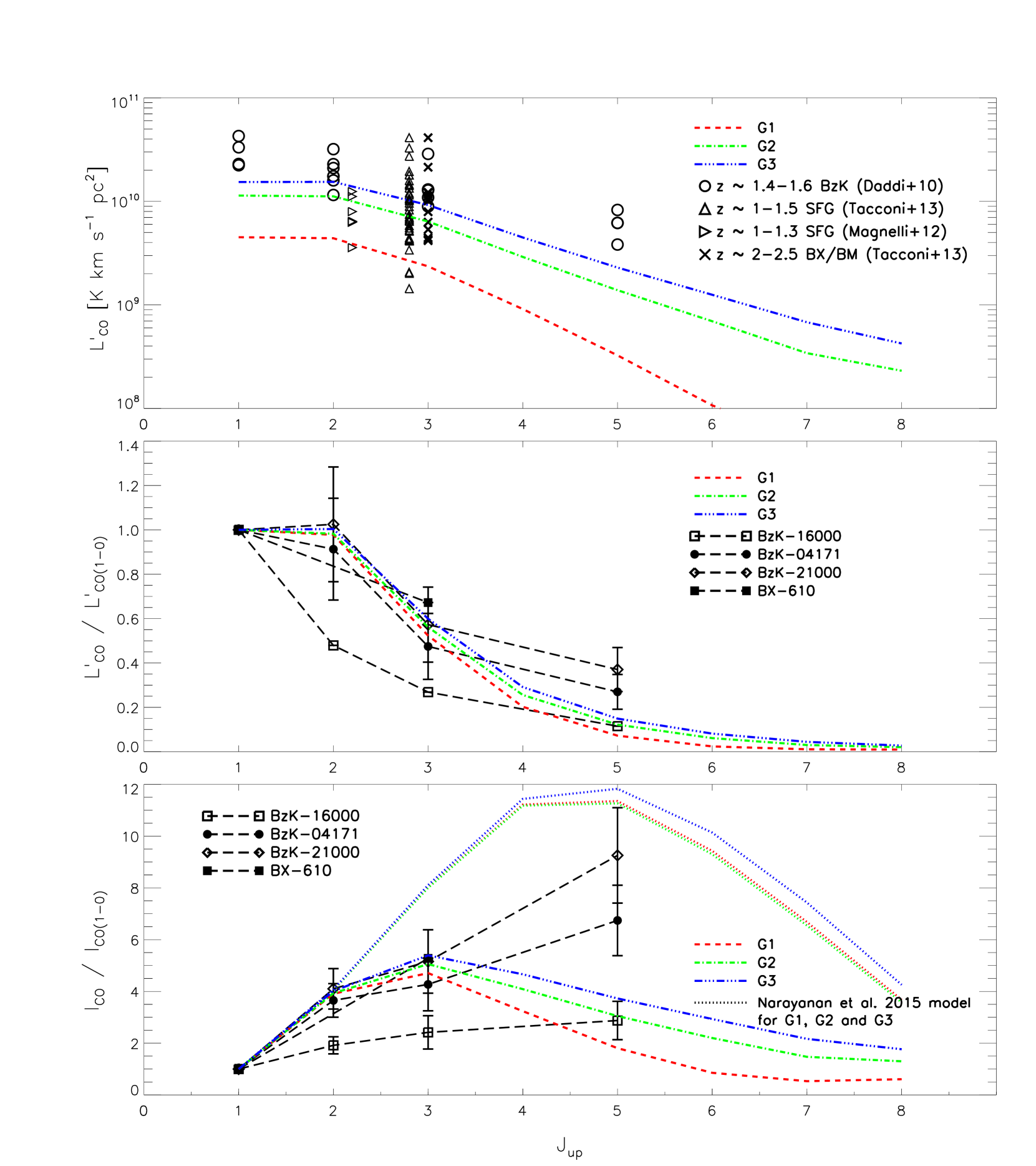
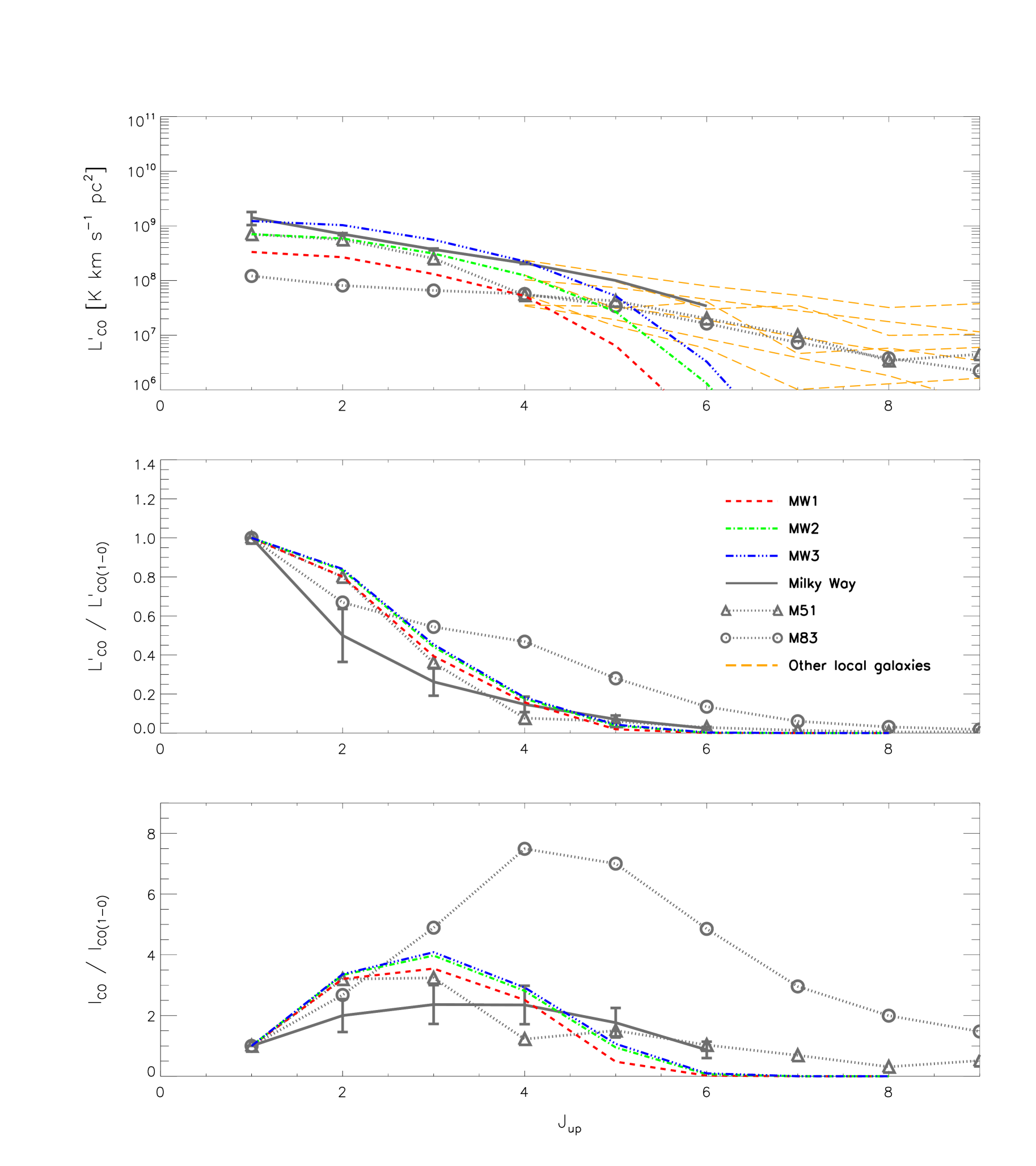
4.4 Global CO line luminosities and spectral line energy distributions

The global CO SLEDs of G1, G2 and G3 are shown in Figure 10 in three different incarnations: 1) total CO line luminosities ($L^{\prime}_{\rm CO_{J,J-1}}$), 2) brightness temperature ratios ($T_{\rm B,CO_{J,J-1}}/T_{\rm B,CO_{1,0}}=L^{\prime}_{\rm CO_{J,J-1}}/L^{\prime}_{\rm CO_{1,0}}$) and 3) line intensity ratios ($I_{\rm CO_{J,J-1}}/I_{\rm CO_{1,0}}=L^{\prime}_{\rm CO_{J,J-1}}/L^{\prime}_{\rm CO_{1,0}}\times\left(\nu_{\rm CO_{J,J-1}}/\nu_{\rm CO_{1,0}}\right)^{2}$). We have also compiled relevant CO observations of normal star-forming galaxies at $z\sim 1-3$ in order to facilitate a comparison with our simulated CO SLEDs. In addition to the $z\sim 1-1.5$ BzK and $z\sim 2-2.5$ BX/BM samples by Daddi et al. (2010) and Tacconi et al. (2013), respectively, this includes 7 star-forming galaxies (SFGs) at $z\sim 1.2$ (Magnelli et al., 2012) and 39 SFGs at $z\sim 1-1.5$ (Tacconi et al., 2013). The galaxies in the sample from Magnelli et al. (2012) are all detected in CO(2$-$1) as well as in Herschel/PACS bands, and have $\log({M_{*}/\mbox{$\rm{M}_{\odot}$}})=10.36-11.31$ and SFR $\sim 29-74$ $\rm{M}_{\odot}$ yr^-1. The $z\sim 1-1.5$ SFG sample from Tacconi et al. (2013) comes from the Extended Growth Strip International Survey (EGS), is covered by the CANDELS and 3D-HST programs ($J-H$ bands and H$\alpha$ respectively), and has $\log({M_{*}/\mbox{$\rm{M}_{\odot}$}})=10.40-11.23$ and SFR $\sim 28-630$ $\rm{M}_{\odot}$ yr^-1.

The $z\sim 2-2.5$ BX/BM galaxies of Tacconi et al. (2013) are not only closest in redshift to our simulated galaxies but also occupy the same region of the SFR$-M_{*}$ plane (see Figure 2). We find that G2 and G3, the two most massive ($M_{*}>10^{11}$ $\rm{M}_{\odot}$) and star-forming (SFR $\gtrsim 80$ $\rm{M}_{\odot}$ yr^-1) galaxies of our simulations, have CO(3$-$2) luminosities of $6.4\times 10^{9}$ and $9.2\times 10^{9}\,{\rm K\,km\,\mbox{s${}^{-1}$}\,pc^{2}}$, respectively, in the range of CO(3$-$2) luminosities of the BX/BM galaxies. G1 is just below this range and about a factor of 4 below the average BX/BM luminosity ($\sim 1.2\pm 0.9\times 10^{10}\,{\rm K\,km\,\mbox{s${}^{-1}$}\,pc^{2}}$). All three simulated galaxies have CO(2$-$1) and CO(3$-$2) luminosities consistent with those of the $z\simeq 1-1.5$ SFGs observed by Magnelli et al. (2012) and Tacconi et al. (2013), which span a range in CO(2$-$1) and CO(3$-$2) luminosity of $(3.6-12.5)\times 10^{9}$ and $(1.4-41.3)\times 10^{9}\,{\rm K\,km\,s^{-1}\,pc^{2}}$, respectively. Finally, we see that the $z\sim 1.5$ BzK galaxies in general have higher CO line luminosities across all observed CO transitions (up to $J_{\rm up}=5$), although at the $J=2-1$ and $J=3-2$ transitions there is overlap with G3. As mentioned in Section 4.1, the molecular gas mass fractions of our galaxies is a factor $\sim 4-5$ below the mean of the observed galaxies at $z\sim 1-2.5$ with which we compare, and we propose this as the main reason for the comparatively low CO luminosities.

Differences in the global CO excitation conditions between G1, G2 and G3 are best seen in the CO(1$-$0) normalised luminosity (and intensity) ratios, i.e., middle (and bottom) panel in Figure 10. The CO SLEDs of all three galaxies follow each other quite closely up to the $J=3-2$ transition where the SLEDs all peak; at $3<J_{\rm up}<7$ the SLEDs gradually diverge. While the metallicity distributions in G1, G2 and G3 are similar (see Figure 15), the rise in $G_{0}^{\prime}$ presents a likely cause to the increasing high-$J$ flux when going from G1 to G3, as higher $G_{0}^{\prime}$ leads to more flux primarily in the $J>4$ transitions (see Figure 17).

Our simulated galaxies are seen to have CO 2$-$1/1$-$0, 3$-$2/1$-$0, and 5$-$4/1$-$0 brightness temperature ratios of $r_{\rm 21}\simeq 1$, $r_{\rm 32}\simeq 0.6$, and $r_{\rm 54}\simeq 0.15$, respectively. The first two ratios compare extremely well with the line ratios measured for BzK$-$4171 and BzK$-$21000, i.e., $r_{\rm 21}\simeq 0.9-1$, and $r_{32}\simeq 0.5-0.6$ (Dannerbauer et al., 2009; Aravena et al., 2010; Daddi et al., 2010, 2015), and suggest that our simulations are able to emulate the typical gas excitation conditions responsible for the excitation of the low-$J$ lines in normal $z\sim 1-3$ SFGs. In contrast, $r_{\rm 54}=0.3-0.4$ observed in BzK$-$4171 and BzK$-$21000 (Daddi et al., 2015), is nearly $2\times$ higher than our model predictions. Daddi et al. (2015) argue that this is evidence for a component of denser and possibly warmer molecular gas, not probed by the low-$J$ lines. In this picture, we would expect CO(4$-3$) to probe both the cold, low-excitation gas as well as the dense and possibly warm star-forming gas traced by the CO(5$-$4) line, and we would expect CO(6$-$5) to be arising purely from this more highly excited phase and thus departing even further from our models.

However, significant scatter in the CO line ratios of main-sequence galaxies is to be expected, as demonstrated by the significantly lower line ratios observed towards BzK$-$16000: $r_{\rm 21}\simeq 0.4$, $r_{\rm 32}\simeq 0.3$, and $r_{\rm 54}\simeq 0.1$ (Aravena et al., 2010; Daddi et al., 2010, 2015) and, in fact, the average $r_{\rm 54}$ for all three BzK galaxies above ($\simeq 0.2$; Daddi et al., 2015) is consistent with our models. It may be that G2 and G3, and perhaps even G1, are more consistent with the CO SLEDs of the bulk $z\sim 1-3$ main-sequence galaxies. We stress, that to date, no $z\sim 1-3$ main sequence galaxies have been observed in the $J=4-3$ nor the $6-5$ transitions, and observations of these lines, along with low- and high-$J$ lines in many more BzK and main-sequence $z\simeq 1-3$ galaxies are needed in order to fully delineate the global CO SLEDs in a statistically robust way.

5 Testing different ISM models

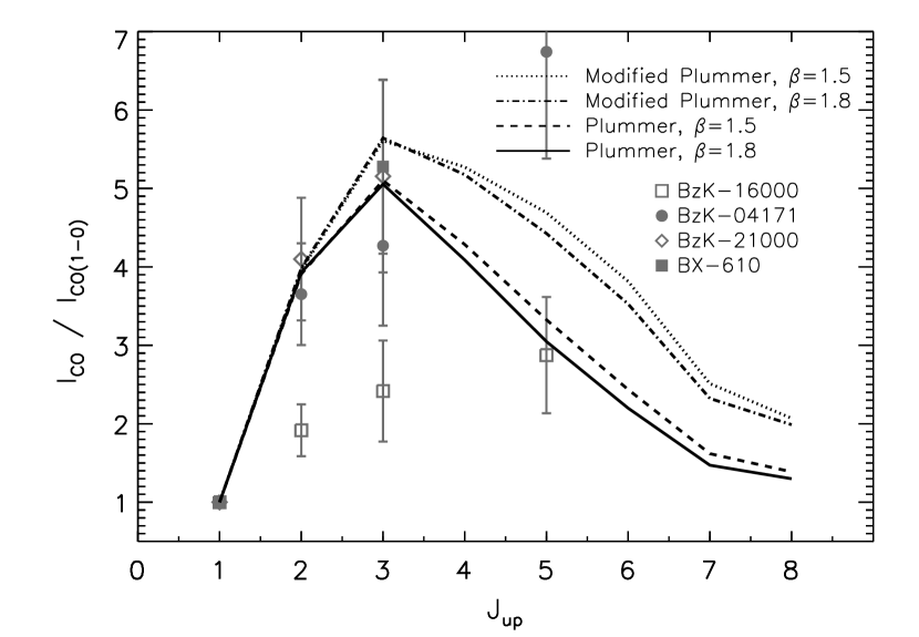
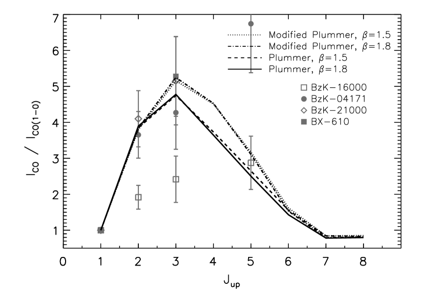
In this section we investigate the effects on our simulation results when adopting i) a more top-heavy GMC mass spectrum with a slope of $\beta=1.5$, ii) a steeper GMC density profile, i.e., a Plummer profile exponent of $-7/2$, and iii) a GMC model grid that includes $P_{\rm{ext}}$ as a fourth parameter. In order to carry out option iii), the GMC model grid was produced for $\mbox{$P_{\rm{ext}}$}/k_{\rm B}=10^{4}\,{\rm cm^{-3}\,K}$ (default), $10^{5.5}\,{\rm cm^{-3}\,K}$ and $10^{6.5}\,{\rm cm^{-3}\,K}$, allowing for a look-up table of CO SLEDs in ($G_{0}^{\prime}$, $m_{\rm GMC}$, $Z^{\prime}$, $P_{\rm{ext}}$) parameter space.

We examine the effects that options i)-iii) have on the global CO SLED of galaxy G2 (Figure 11) and how combinations of option i) and ii) change the values of the global CO-to-H₂ conversion factor for all three simulated galaxies (Table 4). Also, we show the impact that changes ii) and iii) have on the CO SLEDs of the individual GMC grid models in Figures 18 and 19.

Changing the GMC mass spectrum from $\beta=1.8$ to $1.5$ leaves the CO SLED virtually unchanged with only a marginal increase in the line flux ratios for $J_{\rm up}\geq 4$. This holds true regardless of what has been assumed for ii) and iii) (compare solid vs. dashed and dot-dashed vs. dotted curves in Figure 11). Also, changing $\beta$ from 1.8 to 1.5 does not lead to any significant change in $\alpha_{\rm CO}$ (Table 4).

Adopting the modified Plummer density profile with an exponent of $-7/2$ instead of $-5/2$ results in significantly higher global line ratios for $J_{\rm up}\geq 3$ (see dotted vs. dashed curve and dot-dashed vs. solid curves in Figure 11). This is due to the higher central densities achieved for the modified Plummer profile which, as shown in Figure 18, leads to an increase in the excitation of the higher $J$ lines relative to that of the low-$J$ lines. Significantly higher $\alpha_{\rm CO}$ values ($\simeq 3.6\,{\rm\mbox{$\rm{M}_{\odot}$}\,pc^{-2}\,(K\,km\,s^{-1})^{-1}}$) are obtained when adopting a modified Plummer profile (Table 4). These are in excellent agreement with the $\alpha_{\rm CO}$ values inferred for $z\simeq 1.5-2$ BzK galaxies by Daddi et al. (2010). In our simulations, the higher $\alpha_{\rm CO}$ values are due the steeper density profile which leads to smaller GMC sizes and therefore smaller CO$(1-0)$ fluxes (Figure 18) and, ultimately, a lowering of the total CO$(1-0)$ luminosity of the galaxy.

Including external pressures of $\mbox{$P_{\rm{ext}}$}/k_{\rm B}=10^{5.5}\,{\rm cm^{-3}\,K}$ and $10^{6.5}\,{\rm cm^{-3}\,K}$ in the GMC model grid (see Section 3.4.4), means that these pressure values are assigned to GMCs with $\mbox{$P_{\rm{ext}}$}/k_{\rm B}$ in the ranges $10^{4.75}-10^{6}$ and $>10^{6}\,{\rm cm^{-3}\,K}$, respectively. The higher pressures now experienced by these subsets of GMCs results in smaller radii since $R_{\rm GMC}\propto\mbox{$P_{\rm{ext}}$}^{-1/4}$ for a given mass (see eq. 9). Their velocity dispersions and densities increase since $\sigma_{v}\propto P_{\rm ext}^{1/8}$ and $n_{\rm H_{2}}(R=0)\propto P_{\rm ext}^{3/4}$ for a given mass (see eqs. 10 and 11). The net effect this has on the global CO SLED is depicted in the bottom panel of Figure 11. Line ratios with $J_{\rm up}=3$ are lowered, and increasingly so for higher $J$, resulting in a steeper decline at high ($J_{\rm up}\geq 4$) transitions.

Table 4: The global H₂-to-CO conversion factors (in units of ${\rm\mbox{$\rm{M}_{\odot}$}\,pc^{-2}\,(K\,km\,s^{-1})^{-1}}$), averaged over G1, G2, and G3, for combinations of assumptions i) and ii). The pressure has been kept fixed at $\mbox{$P_{\rm{ext}}$}/k_{\rm B}=10^{4}\,{\rm\mbox{cm${}^{-3}$}\,K}$.

	$\beta=1.8$	$\beta=1.5$
Plummer profile	$1.5\pm 0.1$	$1.5\pm 0.1$
Modified Plummer profile	$3.6\pm 0.4$	$3.5\pm 0.5$

Figure 11: Global CO SLEDs of our model galaxy G2 for different choices of ISM prescriptions. Top: For a pressure fixed of $10^{4}\,{\rm\mbox{cm${}^{-3}$}\,K}$. Bottom: Using the $P_{\rm{ext}}$ as a fourth parameter in the GMC model grid (see Section 3.4.4).

6 Comparison with other models

The sub-grid physics implemented by sígame assumes that the scaling-laws and thermal balance equations that have been established for GMCs in our own Galaxy can be applied to the ISM conditions in high-$z$ galaxies. In this respect, sígame does not differ from most other numerical simulations of the molecular line emission from galaxies (e.g., Narayanan et al., 2006; Pelupessy et al., 2006; Greve & Sommer-Larsen, 2008; Christensen et al., 2012; Lagos et al., 2012; Muñoz & Furlanetto, 2013; Narayanan & Krumholz, 2014; Lagos et al., 2012; Popping et al., 2014), although there are of course differences in the range and level of detail of the various sub-grid physics implementations. Here we highlight and discuss some of these differences between sígame and other simulations.

First, however, we compare the sígame CO SLEDs of G1, G2, and G3 with those predicted by other CO emission simulations of similar main-sequence galaxies. A direct comparison can be made with the models presented by Narayanan & Krumholz (2014), where the global CO SLED is parametrised as a function of the luminosity weighted SFR surface density ($\Sigma_{\rm SFR}$). We approximate a luminosity weighted $\Sigma_{\rm SFR}$ by calculating a mean of $\Sigma_{\rm SFR}$ for $1\,{\rm kpc}^{2}$ pixels across the galaxies seen face-on, weighted by the total SFR within the pixels. With this procedure, G1, G2 and G3 have $\Sigma_{\rm SFR}$ of $3.0$, $2.9$ and $3.8\,\mbox{$\rm{M}_{\odot}$~{}yr${}^{-1}$}\,{\rm kpc}^{2}$, respectively, and the resulting CO SLEDs inferred from the Narayanan & Krumholz (2014) parametrisation are shown as dotted lines in the bottom panel of Figure 10. These are seen to peak at $J_{\rm up}=5$ and not $3$ as the sígame CO SLEDs do. Also, the line flux ratios are significantly higher for all transitions above $J_{\rm up}=2$. Both set of models agree on the $r_{21}$ ratio, but follow distinct CO SLED shapes for the remaining transitions. The models also seem to suggest one dominating ISM phase, whereas the observed CO SLED of the BzK galaxies indicate a more complex multi-phased ISM.

Combining a semi-analytical galaxy formation model with a photon-dominated region code, Lagos et al. (2012) made predictions of the CO SLEDs of $z=2$ galaxies as a function of their IR luminosities. They found that for galaxies with infrared luminosities $L_{\rm IR}\sim 10^{11.6}-10^{12.2}\,\mbox{$L_{\odot}$}$ – which is the range found for G1, G2, and G3 if one adopts $L_{\rm IR}/L_{\odot}=\rm{SFR}/[\mbox{$\rm{M}_{\odot}$}\,\rm{yr}^{-1}]\times 10^{10}$ (Kennicutt 1998 for a Chabrier IMF) – the CO SLEDs (when converted to velocity integrated flux ratios in order to compare with the bottom panel of Figure 10) peak at $J=3-2$, in agreement with our model galaxies. However, the line ratios of the CO SLEDs of Lagos et al. (2012) are consistently above ours up to $J_{\rm up}=7$, but cross over our models at $J_{\rm up}=7$ and go below at $J_{\rm up}=8$. In terms of CO line luminosity, our model G1 agrees best with the models of Lagos et al. (2012), lying within the 10-90 percentile ranges ($80\%$ of their galaxy distribution) for the CO luminosities of their sample for $2<J_{\rm up}<8$, but slightly below for the first two transitions and for $J_{\rm up}>7$. G2 and G3, lying roughly a factor 2-4 above G1, are outside the 10-90 percentile ranges of the models from Lagos et al. (2012).

Popping et al. (2014), in their semi-analytical study of MS galaxies at $z=0$, 1.2 and 2, found that for galaxies with far-infrared (FIR) luminosities of $L_{\rm FIR}=10^{11}-10^{12}\,\mbox{$L_{\odot}$}$, the CO SLED peaks at CO(3$-$2) or CO(4$-$3) at $z=0$, but at CO(6$-$5) at $z=2$, as a result of denser and warmer gas in their model galaxies. The CO luminosities of our galaxies G2 and G3 are in broad agreement with the corresponding models by Popping et al. (2014) at CO(4$-$3) and (5$-$4) for similar SFRs. But at $J_{\rm up}<4$ our galaxies are above while at $J_{\rm up}>5$, our galaxies are below those of Popping et al. (2014) up until $J_{\rm up}=9$ where the SLEDs cross again.

$\bullet$ Implementation of $G_{0}^{\prime}$ and $\zeta_{\rm{CR}}$
sígame stands out from most other simulations to date in the way the FUV radiation field and the CR flux that impinge on the molecular clouds are modelled and implemented. Most simulations adopt a fixed, galaxy-wide value of $G_{0}^{\prime}$ and $\zeta_{\rm{CR}}$, scaled by the total SFR or average gas surface density across the galaxy (e.g., Lagos et al., 2012; Narayanan & Krumholz, 2014). sígame refines this scheme by determining a spatially varying $G_{0}^{\prime}$ (and $\zeta_{\rm{CR}}$) set by the local SFRD, as described in Section 3.3. By doing so, we ensure that the molecular gas in our simulations is calorimetrically coupled to the star formation in their vicinity. If we adopt the method of Narayanan & Krumholz (2014) and calculate a global value for $G_{0}^{\prime}$ by calibrating to the MW value, using SFR${}_{\rm MW}=2$ $\rm{M}_{\odot}$ yr^-1 and $G_{\rm 0,MW}=0.6$ Habing, our galaxies would have $G_{0}^{\prime}$ ranging from about $12$ to $42$, whereas, with the SFR surface density scaling of Lagos et al. (2012), global $G_{0}^{\prime}$ values would lie between about $6$ and $9$. For comparison, the locally determined $G_{0}^{\prime}$ in our model galaxies spans a larger range from $0.3$ to $27$ (see Figure 15). Narayanan & Krumholz (2014) determine the global value of $\zeta_{\rm{CR}}$ as $2\times 10^{-17}\mbox{$Z^{\prime}$}\mbox{s${}^{-1}$}$, corresponding to values of $3.7-6.2\times 10^{-17}\mbox{s${}^{-1}$}$ in our model galaxies, when using the mass-weighted mean of $Z^{\prime}$ in each galaxy. Typical values adopted in studies of ISM conditions are around $(1-2)\times 10^{-17}$s^-1 (Wolfire et al., 2010; Glover & Clark, 2012), but again, the local values of $\zeta_{\rm{CR}}$ in our galaxies span a larger range, from $1.3\times 10^{-17}$ to $1.3\times 10^{-15}$ s^-1. Adopting the method of Narayanan & Krumholz (2014) for $G_{0}^{\prime}$ and $\zeta_{\rm{CR}}$ in our galaxies, leads to higher CO luminosities at $J_{\rm up}>2$, but very similar CO$(1-0)$ luminosities which together with slightly reduced molecular gas masses result in smaller $\alpha_{\rm CO}$ factors by about $7-8$ %.

$\bullet$ The molecular gas mass fraction
In sígame the molecular gas mass fraction ($f^{\prime}_{\rm mol}$) is calculated following the work by Pelupessy et al. (2006) (P06), in which $f^{\prime}_{\rm mol}$ depends on temperature, metallicity, local FUV field, and boundary pressure on the gas cloud in question. Other methods exist, such as those of Blitz & Rosolowsky (2006) and Krumholz et al. (2009) (K09). The K09 method, which was adopted by e.g. Narayanan & Krumholz (2014), establishes $f^{\prime}_{\rm mol}$ from local cloud metallicity, dissociating radiation field and column density. 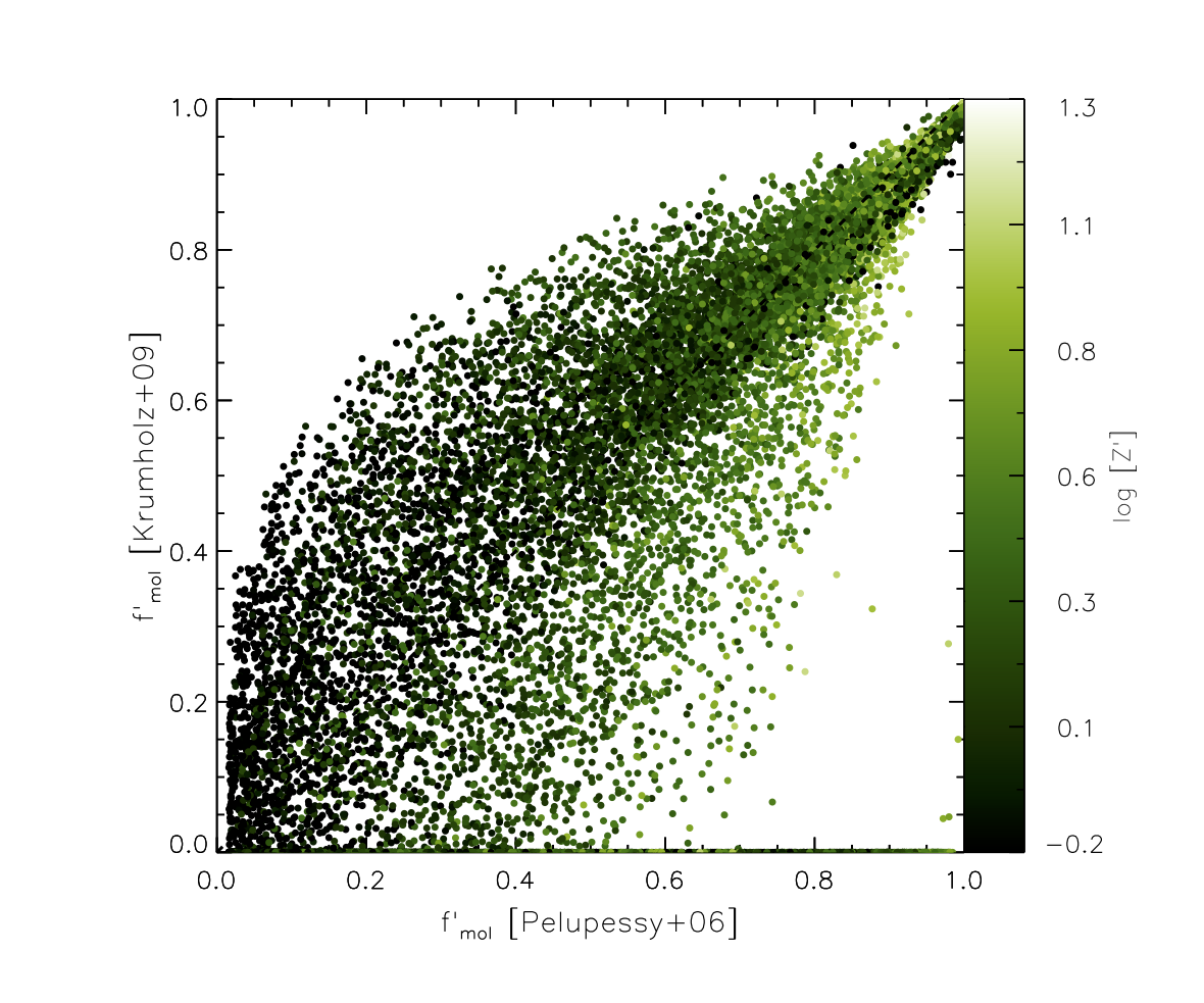In Figure 12 we compare the K09 method to that of P06. The gas surface density that enters in the K09 method was estimated within 1 kpc of each SPH particle, as used in our calculation of $P_{\rm{ext}}$ (see Section 3.3).

The two methods agree for molecular gas fractions $\mathrel{\raise 1.50696pt\hbox{$\scriptstyle>$}\kern-6.00006pt\lower 1.72218pt\hbox{{$\scriptstyle\sim$}}}80\%$, which are seen to be dominated by SPH particles with high metallicities (i.e., $\log\mbox{$Z^{\prime}$}\mathrel{\raise 1.50696pt\hbox{$\scriptstyle>$}\kern-6.00006pt\lower 1.72218pt\hbox{{$\scriptstyle\sim$}}}0.3$). At lower molecular gas fractions the agreement between the two methods exhibit an increasing scatter. Also, systematic, metallicity dependent differences are seen between the two methods. For high metallicity gas, the P06 method gives systematically higher molecular gas fractions than the K09 method. At low metallicities (i.e., $\log\mbox{$Z^{\prime}$}\mathrel{\raise 1.50696pt\hbox{$\scriptstyle<$}\kern-6.00006pt\lower 1.72218pt\hbox{{$\scriptstyle\sim$}}}0.2$) the K09 method tends to result in higher molecular gas fractions than P06. The above is the result of the K09 method having a much weaker dependance on $Z^{\prime}$ Krumholz et al. (2009) than the P06 method (see Section 3.3). Despite these differences, we find that using the K09 instead of the P06 method does not change the total molecular gas mass significantly: $f_{\rm mol}$ for G1, G2 and G3 goes from 12.2, 10.0, 9.2 % to 11.4, 10.7 and 10.3 %, respectively.

Figure 12: Comparison of two methods for calculating the molecular gas mass fraction, $f^{\prime}_{\rm mol}$, of SPH particles in G1: That of Pelupessy et al. (2006) with external cloud pressure derived from hydrostatic mid-plane equilibrium as done in this work (abscissa) and that of Krumholz et al. (2009) (ordinate) used by e.g., Narayanan & Krumholz (2014), color-coded by metallicity.

A common feature of the above Hi $\longrightarrow\mbox{{\sc H}${}_{2}$}$ prescriptions is that they assume an instantaneous Hi to H₂ conversion. However, as pointed out by Pelupessy et al. (2006), the typical timescales for H₂ cloud formation are of order $\sim 10^{7}$ yr, which are comparable to the time-scales of a number of processes, such as cloud-cloud collisions and star formation, that can potentially alter or even fully disrupt typical molecular clouds and drive H₂ formation/destruction in both directions. Ideally, therefore, a comprehensive modeling of the Hi $\longrightarrow\mbox{{\sc H}${}_{2}$}$ transition should be time-dependent. Relying on the findings of Narayanan et al. (2011) and Krumholz & Gnedin (2011), the static solution for H₂ formation is a valid approximation for $\mbox{$Z^{\prime}$}>0.01$, which is the case for the three model galaxies studied here.

$\bullet$ CO abundance
sígame assumes a constant CO abundance relative to H₂, which for the simulations presented in this paper was set to the Galactic CO abundance, i.e., $[{\rm CO}/\mbox{{\sc H}${}_{2}$}]=2\times 10^{-4}$. In reality, H₂ gas can self-shield better than the CO gas, creating an outer region or envelope of ‘CO-dark’ gas (Bolatto et al., 2008). Observations in the MW by Pineda et al. (2013) indicate that the amount of dark gas grows with decreasing metallicity and the resulting absence of CO molecules. By modeling a dynamically evolving ISM with cooling physics and chemistry incorporated on small scales, Smith et al. (2014) showed that in a typical MW-like disk of gas, the CO-dark gas mass fraction, $f_{\rm DG}=$, defined as having integrated CO intensity $W_{\rm CO}<0.1$ K km s^-1, is about $42$ %, but up to $62$ % in a radiation field ten times that of the solar neighbourhood. While Smith et al. (2014) kept metallicity fixed to solar, Wolfire et al. (2010) found $f_{\rm DG}$ values of about $0.5-0.7$ for the low metallicity cases with $\mbox{$Z^{\prime}$}=0.5$ in $10^{6}$ $\rm{M}_{\odot}$ clouds immersed in the local interstellar radiation field. Recently, Bisbas et al. (2015) argued that CR ionization rates of $10-50\times\zeta_{\rm{CR,MW}}$ can effectively destroy most CO in GMCs.

Thus, it is expected that $[{\rm CO}/\mbox{{\sc H}${}_{2}$}]$ is lower in regions of low metallicity and/or intense FUV and CR fields, effectively leading to underestimates of the $\alpha_{\rm CO}$ conversion factor when not accounted for in models. Since in this paper we have restricted our simulations to main-sequence galaxies with solar or higher than solar metallicities, adopting a constant Galactic $[{\rm CO}/\mbox{{\sc H}${}_{2}$}]$ seems a reasonable choice, but see Lagos et al. (2012), Narayanan et al. (2012) and Narayanan & Krumholz (2014) for alternative approaches.

$\bullet$ GMC density and thermal structure
When solving for the temperature structure of each GMC, sígame includes only the most dominant atomic and molecular species in terms of heating and cooling efficiencies. sígame also ignores heating via X-ray irradiation and turbulence. In particular, it has been shown with models that turbulent heating can completely control the mean temperature of molecular clouds, exceeding the heating from cosmic rays (Pan & Padoan, 2009). Our comparison of observed CO SLEDs at $z=2$ with those of sígame, suggest that our simulations are missing a warm gas component, which could be explained, at least in part, by the exclusion of turbulent heating. We have, however, checked our $T_{\rm{k}}$ $-$$n_{\rm{H}_{2}}$ curves in Figure 16 against those of Glover & Clark (2012), who performed time-resolved, high-resolution ($\delta m\simeq 0.05-0.5\,\mbox{$\rm{M}_{\odot}$}$) SPH simulations of individual FUV irradiated molecular clouds using a chemical network of 32 species (see their Figure 2). Overall, there is great similarity in the $T_{\rm{k}}$ vs. $n_{\rm{H}_{2}}$ behaviour of the two sets of simulations. This includes the same main trend of decreasing temperature with increasing hydrogen density, as well as the local increase in $T_{\rm{k}}$ at $\sim 10^{3}-10^{4}$ cm^-3 and the subsequent decrease to $\mbox{$T_{\rm{k}}$}<10$ K at $\mbox{$n_{\rm{H}_{2}}$}>10^{5.5}$ cm^-3. Thus, our GMCs models, despite their simplified density profiles and chemistry, seem to agree well with much more detailed simulations.

7 Summary

In this paper we have presented sígame, a code that simulates the molecular line emission of galaxies via a detailed post-processing of the outputs from cosmological SPH simulations. A sequence of sub-grid prescriptions are applied to a simulation snapshot in order to derive the molecular gas density and temperature from the SPH particle information, which includes SFR, gas density, temperature and metallicity.

A key aspect of sígame is the localised coupling between the star formation and the energetics of the ISM, where the strength of the local FUV radiation field and CR ionization rate that impinge and heat a cloud scales with the local star formation rate density. The radial temperature profile of each GMC is calculated by balancing the heating rate with cooling from H₂, CO, [Oi], and [Cii] lines in addition to gas-dust interactions. In these thermal balance calculations, sígame takes into account the local enrichment of the gas, which is a critical parameter for the cooling rates. The CO emission line spectrum from a grid of GMC models is calculated using the 3D radiative transfer code lime.

We used sígame to create line emission velocity-cubes of the full CO rotational ladder for three cosmological N-body/SPH simulations of massive ($M_{*}\gtrsim 10^{10.5}\,\mbox{$\rm{M}_{\odot}$}$) main-sequence galaxies at $z=2$.

Molecular gas is produced more efficiently towards the centre of each galaxy, and while Hi surface gas densities (including helium) do not exceed $\sim 100$ $\rm{M}_{\odot}$  pc^-2 anywhere in the disk, central molecular gas surface densities reach $\sim 1000$ $\rm{M}_{\odot}$  pc^-2 on spatial scales of $100\,{\rm pc}\times 100\,{\rm pc}$, in good agreement with observations made at similar spatial resolution. This strong increase in molecular surface density is brought on by a similar increase in total gas surface density, overcoming the increase in photo-dissociating FUV field towards the centre of each galaxy.

Turning to the CO emission, the velocity-integrated moment 0 maps reveal distinct differences in the various transitions as molecular gas tracers. The morphology of molecular gas in our model galaxies is well reproduced in CO(1-0), but going to higher transitions, the region of CO emitting gas shrinks towards the galaxy centres. The global CO SLEDs of our simulated galaxies all peak at $J=3-2$. Recent CO$(5-4)$ observations of $z\sim 1.5$ BzK galaxies seem to suggest that these galaxies actually peak at higher $J$. The CO$(3-2)$ line luminosities of our model galaxies are within the range of corresponding observed samples at redshifts $z\sim 1-2.5$, however on the low side. In particular, the model galaxies are below or at the CO luminosities of BzK-selected galaxies of comparable mass and SFR but at $z\sim 1.5$. The low luminosities are most likely a consequence of molecular gas mass fractions in our galaxies being about $\sim 4-5$ times below the observed values in the star-forming galaxies at $z=1-2.5$ used to compare with.

Combining the derived H₂ gas masses with the CO$(1-0)$ line emission found, we investigate local variations in the CO-H₂ conversion factor $\alpha_{\rm CO}$. The radial $\alpha_{\rm CO}$ profiles all show a decrease towards the galaxy centres, dropping by a factor of $\sim 1.2$ in the central $R\leq 2$ kpc region compared to the disk average, the main driver being the FUV field rather than a gradient in density or metallicity. Global $\alpha_{\rm CO}$ factors range from $1.4$ to $1.6$ $\rm{M}_{\odot}$  pc^-2 (K km s^-1)^-1 or about $0.3$ times the MW value, but closer to values for $z\sim 1.5$ normal star-forming galaxies identified with the BzK colour criteria. Changing the GMC properties from what is observed in the MW and local galaxies to a steeper GMC density profiles and/or a shallower GMC mass spectra, resulted in elevated $\alpha_{\rm CO}$ values of up to $0.9$ times the MW value.

The CO luminosity ratios of CO 3$-$2/1$-$0 and 7$-$6/1$-$0 ($r_{32}$ and $r_{76}$ respectively) drop off in radius about where the FUV radiation drops in intensity, and are thus likely controlled by the FUV field as is $\alpha_{\rm CO}$. The global ratios of $r_{21}\simeq 1$ and $r_{32}\simeq 0.6$ agree very well with observations of BzK galaxies, while the $r_{54}$ of about $0.15$ is low compared to recent observations in BzK$-$4171 and BzK$-$21000. The low flux from high CO transitions in our models compared to observations could be explained, at least in part, by our omission of turbulent heating in sígame. However, more observations of $J_{\rm up}>3$ lines towards high-$z$ main-sequence galaxies, such as the BzKs, are still needed in order to determine the turn-over in their CO SLEDs and better constrain the gas excitation.

Finally, we note that sígame in principle is able to simulate the emission from a broad range of molecular and atomic lines in the far-IR/mm wavelength regime provided measured collision rates exist, such as those found in the LAMDA database. In the future, we aim to apply sígame to a larger and more diverse sample of galaxies, possibly at higher redshift, and explore the emission from other important ISM diagnostic lines.

Appendix A Thermal balance of the atomic gas phase

As explained in § 3.2, we cool the initial hot SPH gas by requiring: $\mbox{$\Gamma_{\rm{CR,H}\textsc{i}}$}=\mbox{$\Lambda_{\rm{atoms+ions}}$}+\mbox{$\Lambda_{\rm{rec}}$}+\mbox{$\Lambda_{\rm{f-f}}$}$.

$\Gamma_{\rm{CR,H}\textsc{i}}$ is the heating rate of the atomic gas due to cosmic ray ionizations (Draine, 2011):

$$\mbox{$\Gamma_{\rm{CR,H}\textsc{i}}$}= 1.03\times 10^{-27}\mbox{$n_{\rm{H}\textsc{i}}$}\left(\frac{\mbox{$\zeta_{\rm{CR,H}\textsc{i}}$}}{10^{-16}}\right)$$ (17)

$$\times\left[1+4.06\left(\frac{\mbox{$x_{\rm{e}}$}}{\mbox{$x_{\rm{e}}$}+0.07}\right)^{1/2}\right]~{}~{}{\rm erg\,cm^{-3}\,s^{-1}},$$

where $\zeta_{\rm{CR,H}\textsc{i}}$ is the primary CR ionization rate of Hi atoms (determined locally in our simulations according to eq. 12), and $x_{\rm{e}}$ is the hydrogen ionization fraction calculated with a procedure kindly provided by I. Pelupessy; see also Pelupessy (2005). The term containing $x_{\rm{e}}$ in eq. 17 accounts for the fact that in highly ionised gas, electrons created by primary CR ionization have a high probability of transferring their kinetic energy into heat via long-range Coulomb scattering off free electrons. For low ionization gas, this term becomes insignificant as a higher fraction of the energy of the primary electrons goes to secondary ionizations or excitation of bound states instead of heating.

$\Lambda_{\rm{atoms+ions}}$ is the total cooling rate due to line emission from H, He, C, N, O, Ne, Mg, Si, S, Ca, and Fe, calculated using the publically available code of Wiersma et al. (2009) which takes $T_{\rm{k}}$, $n_{\rm{H}}$ and the abundances of the above elements as input. Wiersma et al. (2009) compute the cooling rates with the photoionization package CLOUDY assuming CIE. They also adopt a value for the meta-galactic UV and X-ray field equal to that expected at $z\sim 2$ (Haardt & Madau, 2001). At $z\sim 2$, the emission rate of Hi ionizing radiation is higher by a factor of about $\sim 30$ than at $z=0$ (Puchwein et al., 2015), and thus plays an important role in metal line cooling calculations.

$\Lambda_{\rm{rec}}$ is the cooling rate due to hydrogen recombination emission (Draine, 2011):

$$\mbox{$\Lambda_{\rm{rec}}$}=\alpha_{B}\mbox{$n_{\rm{e}}$}\mbox{$n_{\rm{H}^{+}}$}\langle E_{rr}\rangle~{}~{}{\rm ergs\,cm^{-3}\,s^{-1}},$$ (18)

where $\alpha_{B}$ is the radiative recombination rate for hydrogen in the case of optically thick gas in which ionizing photons emitted during recombination are immediately re-absorbed. We adopt the approximation for $\alpha_{B}$ given by Draine (2011):

$$\alpha_{\rm B}=2.54\times 10^{-13}T_{4}^{\left(-0.8163-0.0208\ln T_{4}\right)}~{}~{}{\rm cm}^{3}\,\mbox{s${}^{-1}$},$$ (19)

where $T_{4}$ is defined as $\mbox{$T_{\rm{k}}$}/10^{4}$ K. The density of ionised hydrogen, $n_{\rm{H}^{+}}$, is set equal to the electron density, $n_{\rm{e}}$, and $E_{rr}$ is the corresponding mean kinetic energy of the recombining electrons:

$$\langle E_{rr}\rangle=\left[0.684-0.0416\,\ln T_{4}\right]\,k_{\rm B}\mbox{$T_{\rm{k}}$}~{}~{}{\rm ergs}.$$ (20)

$\Lambda_{\rm{f-f}}$ is the cooling rate due to free-free emission from electrons in a pure H plasma (i.e., free electrons scattering off H⁺), and is given by (Draine, 2011):

$$\mbox{$\Lambda_{\rm{f-f}}$}=0.54T_{4}^{0.37}k_{B}\mbox{$T_{\rm{k}}$}\mbox{$n_{\rm{e}}$}\mbox{$n_{\rm{H}^{+}}$}\alpha_{\rm B}~{}~{}\rm{ergs\,cm^{-3}\,s^{-1}},$$ (21)

where the recombination rate, $\alpha_{\rm B}$, is calculated in the same way as for $\Lambda_{\rm{rec}}$.

Figure 13 shows the above heating and cooling rates pertaining to two example SPH particles with similar initial temperatures ($\sim 10^{4}\,{\rm K}$). Because of different ambient conditions (i.e., $n_{\rm{H}\textsc{i}}$, $x_{\rm{e}}$, $Z^{\prime}$, and $\zeta_{\rm{CR}}$) the equilibrium temperature solutions for the two gas particles end up being significantly different.

Figure 13: Heating and cooling rates as functions of temperature for two SPH gas particles with [$\mbox{$n_{\rm{H}}$}=14.62$ cm^-3, $\mbox{$\zeta_{\rm{CR}}$}=4.02\times 10^{-16}$ s^-1, $x_{\rm{e}}$ ($T_{\rm k,SPH}=8892\,K)=0.006$] (left) and [$\mbox{$n_{\rm{H}}$}=0.09$ cm^-3, $\mbox{$\zeta_{\rm{CR}}$}=3.92\times 10^{-16}$ s^-1, $x_{\rm{e}}$ ($T_{\rm k,SPH}=5649\,K)=0.001$] (right). In both cases the metal line emission is the main cooling agent. The left-hand side plot illustrates the case of an SPH particle of high gas density and metallicity, leading to relatively efficient metal line cooling and in a low equilibrium temperature of $\mbox{$T_{\rm{k}}$}=37$ K. The right-hand side plot shows a case of lower density and metallicity causing less cooling by metal lines, hence a higher equilibrium temperature despite a slightly lower CR heating rate. The dashed vertical lines in the two panels indicate the original SPH gas temperatures of the SPH particles, and the solid vertical lines mark their final equilibrium temperatures.

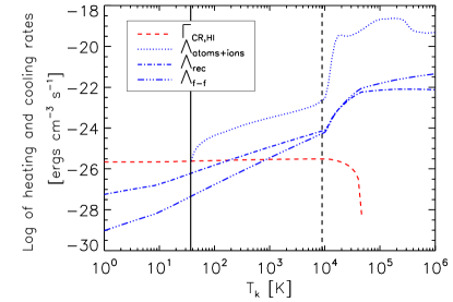
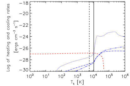
Appendix B Thermal balance of the molecular gas phase

As described in Section 3.4 SÍGAME assumes that the molecular gas resides exclusively in giant molecular clouds that have Plummer radial density profiles (i.e., given by eq. 11). Throughout the clouds the gas temperature is solved for according to the heating and cooling equilibrium requirement $\mbox{$\Gamma_{\rm{PE}}$}+\mbox{$\Gamma_{\rm{CR,H}_{2}}$}=\mbox{$\Lambda_{\rm{H}_{2}}$}+\mbox{$\Lambda_{\rm{CO}}$}+\mbox{$\Lambda_{\rm{C}\rm{\textsc{ii}}}$}+\mbox{$\Lambda_{\rm{O}\rm{\textsc{i}}}$}$+$\Lambda_{\rm{gas-dust}}$ (eq. 14).

$\Gamma_{\rm{PE}}$ is the heating rate of the gas due to photo-electric ejection of electrons from dust grains by FUV photons, and is given by (Bakes & Tielens, 1994):

$$\mbox{$\Gamma_{\rm{PE}}$}=10^{-24}\epsilon\mbox{$G_{0{\rm,att}}^{\prime}$}\mbox{$n_{\rm{H}}$}~{}~{}{\rm\mbox{ergs\,cm${}^{-3}$\,s${}^{-1}$}},$$ (22)

where $G_{0{\rm,att}}^{\prime}$ is the local attenuated FUV field in Habing units, derived following eq. 13, and $\epsilon$ is the heating efficiency:

$$\epsilon= \frac{4.87\times 10^{-2}}{1+4\times 10^{-3}(\mbox{$G_{0{\rm,att}}^{\prime}$}T^{0.5}/n_{e})^{0.73}}$$ (23)

$$+\frac{3.65\times 10^{-2}}{1+4\times 10^{-3}(\mbox{$G_{0{\rm,att}}^{\prime}$}T^{0.5}/n_{e})^{0.73}},$$

where $n_{\rm{e}}$ is the electron density, calculated as $x_{\rm{e}}$$n_{\rm{H}}$, with $x_{\rm{e}}$ again calculated using the procedure of I. Pelupessy.

$\Gamma_{\rm{CR,H}_{2}}$ is the heating rate by cosmic rays traveling through molecular gas (Stahler & Palla, 2005):

$$\mbox{$\Gamma_{\rm{CR,H}_{2}}$}=1.068\times 10^{-24}\left(\frac{\mbox{$\zeta_{\rm{CR,H}_{2}}$}}{10^{-16}}\right)\left(\frac{\mbox{$n_{\rm{H}_{2}}$}}{10^{3}\,\mbox{cm${}^{-3}$}}\right)~{}~{}{\rm ergs\,cm^{-3}\,s^{-1}}$$ (24)

where $\zeta_{\rm{CR,H}_{2}}$ is the local CR primary ionization rate of H₂ molecules, which is approximately $1.6\times$ higher that of Hi atoms (Stahler & Palla, 2005).

$\Lambda_{\rm{H}_{2}}$ is the H₂ line cooling rate, and we use the parameterization made by Papadopoulos et al. (2014) that includes the two lowest H₂ rotational lines (S(0) and S(1), the only lines excited for $\mbox{$T_{\rm{k}}$}\lesssim 1000\,{\rm K}$):

$$\mbox{$\Lambda_{\rm{H}_{2}}$}= 2.06\times 10^{-24}\frac{n_{\rm H_{2}}}{1+{\rm r}_{\rm op}}\left[1+\frac{1}{5}e^{510{\rm K}/T_{\rm k}}\left(1+\frac{n_{0}}{n_{\rm H_{2}}}\right)\right]^{-1}$$ (25)

$$\times(1+R_{10})\rm{\,ergs\,cm^{-3}\,s^{-1}},$$

where ${\rm R}_{10}$ is defined as:

$${\rm R}_{10}=26.8\,{\rm r}_{\rm op}\left[\frac{1+(1/5)e^{510{\rm K}/T_{\rm k}}\left(1+\frac{n_{0}}{n_{\rm H_{2}}}\right)}{1+(3/7)e^{845\,{\rm K}/T_{\rm k}}\left(1+\frac{n_{1}}{n_{\rm H_{2}}}\right)}\right],$$ (26)

and $n_{\rm 0}\sim 54$ cm^-3 and $n_{\rm 1}\sim 10^{3}$ cm^-3 are the critical densities of the S(0):2-0 and S(1):3-1 rotational lines. ${\rm r}_{\rm op}$ is the ortho-H₂/para-H₂ ratio (set to 3 which is the equilibrium value).

For the cooling rates due to the [C ii]$158\,{\rm\mu m}$ and [O i]$63\,{\rm\mu m}$+$146\,{\rm\mu m}$ fine-structure lines we adopt the parameterizations by Röllig et al. (2006). The C ii cooling rate ($\Lambda_{\rm{C}\rm{\textsc{ii}}}$) is:

$$\mbox{$\Lambda_{\rm{C}\rm{\textsc{ii}}}$}= 2.02\times 10^{-24}n\mbox{$Z^{\prime}$}$$ (27)

$$\times\left[1+\frac{1}{2}e^{92{\rm K}/T_{\rm k}}\left(1+1300/\mbox{$n_{\rm{H}}$}\right)\right]^{-1}~{}~{}{\rm ergs\,cm^{-3}\,s^{-1}},$$

where a carbon to hydrogen abundance ratio that scales with metallicity according to $\chi_{\rm[C]}=1.4\times 10^{-4}$ $Z^{\prime}$ is assumed. For the parameterization of the O i cooling rate ($\mbox{$\Lambda_{\rm{O}\rm{\textsc{i}}}$}=\Lambda_{63\mu\rm{m}}+\Lambda_{146\mu\rm{m}}$) we refer to eqs. A.5 and A.6 in Röllig et al. (2006) and simply note that we adopt (in accordance with Röllig et al., 2006) an oxygen to hydrogen abundance ratio of $\chi_{\rm[O]}=3\times 10^{-4}\,\mbox{$Z^{\prime}$}$.

$\Lambda_{\rm{CO}}$ is the cooling rate due to CO rotational transitions. We use the parameterization provided by Papadopoulos & Thi (2013):

$$\mbox{$\Lambda_{\rm{CO}}$}=4.4\times 10^{-24}\left(\frac{n_{\rm H_{2}}}{10^{4}}\right)^{3/2}\left(\frac{T_{\rm k}}{10\,{\rm K}}\right)^{2}\left(\frac{\chi_{\rm CO}}{\chi_{\rm[C]}}\right)\,{\rm ergs\,cm^{-3}\,s^{-1}},$$ (28)

where $\chi_{\rm CO}/\chi_{\rm[C]}$ is the relative CO to neutral carbon abundance ratio, the value of which we determine by interpolation, assuming that $\chi_{\rm CO}/\chi_{\rm[C]}=(0.97,0.98,0.99,1.0)$ for $\mbox{$n_{\rm{H}_{2}}$}=5\times 10^{3},10^{4},10^{5},10^{6}$ cm^-3, respectively (Papadopoulos & Thi, 2013).

$\Lambda_{\rm{gas-dust}}$ is the cooling rate due to gas-dust interactions and is given by (Papadopoulos et al., 2011):

$$\mbox{$\Lambda_{\rm{gas-dust}}$}=3.47\times 10^{-33}\mbox{$n_{\rm{H}}$}^{2}\sqrt{\mbox{$T_{\rm{k}}$}}(\mbox{$T_{\rm{k}}$}-T_{\rm dust})\,{\rm ergs\,cm^{-3}\,s^{-1}},$$ (29)

where the dust temperature ($T_{\rm dust}$) is calculated using eq. 15 (Section 3.4.3).

Figure 14: Equilibrium heating (red curves) and cooling (blue curves) rates of the gas as functions of H₂ density for two different GMC models with [$\mbox{$m_{\rm{GMC}}$}=10^{4}$ $\rm{M}_{\odot}$, $\mbox{$Z^{\prime}$}=1$, $\mbox{$G_{0}^{\prime}$}=27$, $\mbox{$\zeta_{\rm{CR}}$}=1.35\times 10^{-15}\,\mbox{s${}^{-1}$}$, $\mbox{$P_{\rm{ext}}$}=10^{4}\,$K cm^-3 ] (left) and [$\mbox{$m_{\rm{GMC}}$}=10^{4}$ $\rm{M}_{\odot}$, $\mbox{$Z^{\prime}$}=63$, $\mbox{$G_{0}^{\prime}$}=1$, $\mbox{$\zeta_{\rm{CR}}$}=5\times 10^{-17}\,\mbox{s${}^{-1}$}$, $\mbox{$P_{\rm{ext}}$}=10^{4}\,$K cm^-3 ] (right). In the case of high FUV and CR radiation fields but low metallicity (left), the heating is dominated by cosmic ray heating (red solid) in the inner region ($\mbox{$n_{\rm{H}_{2}}$}\gtrsim 1500$ cm^-3) and photoelectric heating (red dotted) in the outer region. Cooling is dominated by gas-dust interactions (blue dashed) in the inner region ($\mbox{$n_{\rm{H}_{2}}$}\gtrsim 10000$ cm^-3) and by [Cii] as well as H₂ line cooling (blue long-dashed and dotted) in the outer region. In the opposite case of low FUV and CR radiation fields but high metallicity (right), the same heating and cooling mechanisms are dominating the energy balance throughout the cloud, except in the inner region, where cooling by CO line emission (blue solid) is more important than it is in the case of low metallicity.

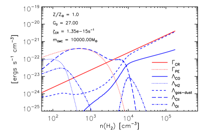
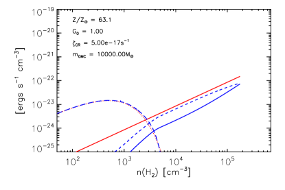
Appendix C GMC models

Each SPH particle is divided into several GMCs as described in § 3.4.1, and we derive the molecular gas density and temperature within each from three basic parameters which are SFR density, GMC mass, $m_{\rm{GMC}}$, and metallicity, $\mbox{$Z^{\prime}$}/Z_{\odot}$. Derived from these basic parameters are the far-UV and cosmic ray field strengths, the H₂ gas mass fraction of each SPH particles, as well as the GMC properties used to derive the CO excitation and emission; H₂ density and temperature. Histograms of the basic parameters are shown in Figure 15, while properties derived thereof can be found in Figure 16.

Figure 15: Mass-weighted histograms of the basic parameters of the GMCs in G1 (red solid), G2 (green dashed), and G3 (blue dotted). From top left and clockwise: the local far-UV field ($G_{0}^{\prime}$) (and CR ionization rate since $\mbox{$\zeta_{\rm{CR}}$}\propto\mbox{$G_{0}^{\prime}$}$), GMC mass ($m_{\rm{GMC}}$), metallicity ($Z^{\prime}$) and external pressure ($P_{\rm{ext}}$). Black vertical lines indicate the $G_{0}^{\prime}$, $m_{\rm{GMC}}$, $Z^{\prime}$, $P_{\rm{ext}}$-values for which $\mbox{$T_{\rm{k}}$}-\mbox{$n_{\rm{H}_{2}}$}$ curves were calculated (see Figure 16) – a total of 630 GMCs which make up our grid GMC models. Each GMC in the galaxies is assigned the $\mbox{$T_{\rm{k}}$}-\mbox{$n_{\rm{H}_{2}}$}$ curve of the GMC model at the closest grid point.

Figure 16: Kinetic temperature versus H₂ density curves for 80 out of the 630 grid model GMCs that span the full ($G_{0}^{\prime}$, $M_{\rm GMC}$, $Z^{\prime}$) parameter space set by and marked on top of the distributions in Figure 15 (see also Section 3.4.4) for a pressure of $\mbox{$P_{\rm{ext}}$}=10^{4}$ K cm^-3. The grid model most often assigned to GMCs in G1 is indicated by the red dashed curve in the highlighted panel and corresponds to $\mbox{$G_{0}^{\prime}$}=7.0$ ($\mbox{$\zeta_{\rm{CR}}$}=3.5\times 10^{-16}$ s^-1), $\log\mbox{$m_{\rm{GMC}}$}/\mbox{$\rm{M}_{\odot}$}=4.25$, and $\mbox{$Z^{\prime}$}=3.2$. In general, higher metallicity (from top to bottom) leads to more cooling via emission lines of ions, atoms and molecules, and hence lower temperatures. On the other hand, higher UV and CR fields (from left to right) cause more heating and therefore higher $T_{\rm{k}}$. The decreasing trend of $T_{\rm{k}}$ with higher values of $n_{\rm{H}_{2}}$ is mainly caused by the gradual attenuation of the UV field as one moves into the cloud. The ‘bump’ at $\mbox{$n_{\rm{H}_{2}}$}\sim 10^{3}-10^{4}$ cm^-3 corresponds to the transition from CII line cooling to the less efficient CO line cooling at higher densities. At densities above $\mbox{$n_{\rm{H}_{2}}$}=10^{4}$ cm^-3, gas-dust interactions set in and eventually cools the gas down to the CMB temperature in all GMC cores.

Figure 17: CO SLEDs obtained with lime for the 80 model GMCs whose $\mbox{$T_{\rm{k}}$}-\mbox{$n_{\rm{H}_{2}}$}$ curves are shown in Figure 16. The CO SLED used most often in G1 is shown as the red dashed curve in the highlighted panel. These CO SLEDs were made for a fixed external pressure of $\mbox{$P_{\rm{ext}}$}/k_{\rm B}=10^{4}\,{\rm\mbox{cm${}^{-3}$}\,K}$ and a default Plummer density profile.

Figure 18: CO SLEDs obtained with lime for the same [$G_{0}^{\prime}$,$Z^{\prime}$] values as shown in the panels of Figure 17 for Plummer density profiles with power-law index $-5/2$ (solid curve) and $-7/2$ (dashed curve). In all panels, the external pressure has been fixed to $\mbox{$P_{\rm{ext}}$}/k_{\rm B}=10^{4}\,{\rm\mbox{cm${}^{-3}$}\,K}$ and the GMC mass to $\mbox{$m_{\rm{GMC}}$}=10^{4.25}\,{\rm\mbox{$\rm{M}_{\odot}$}}$.

Figure 19: CO SLEDs obtained with lime for the same [$G_{0}^{\prime}$,$Z^{\prime}$] values as shown in the panels of Figure 17 for $\mbox{$P_{\rm{ext}}$}/k_{\rm B}=10^{4}\,{\rm cm^{-3}\,K}$ (solid curves), $10^{5.5}\,{\rm cm^{-3}\,K}$ (dashed curves), and $10^{6.5}\,{\rm cm^{-3}\,K}$ (dot-dashed curves). In all panels, the GMC mass is fixed to $10^{4.25}\,\mbox{$\rm{M}_{\odot}$}$. Higher pressure environments are seen to lead to a decrease in luminosity for all transitions.

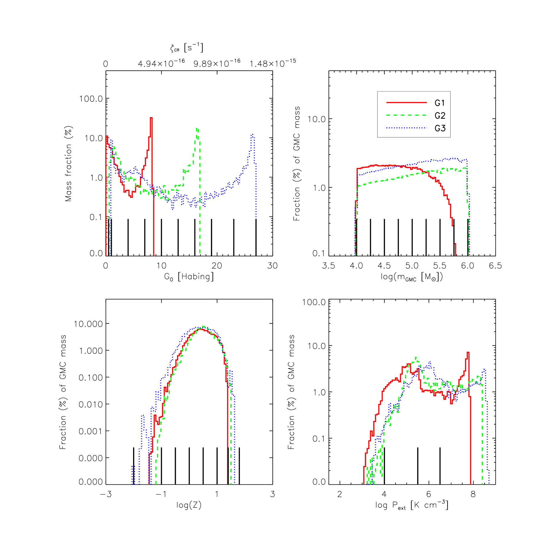
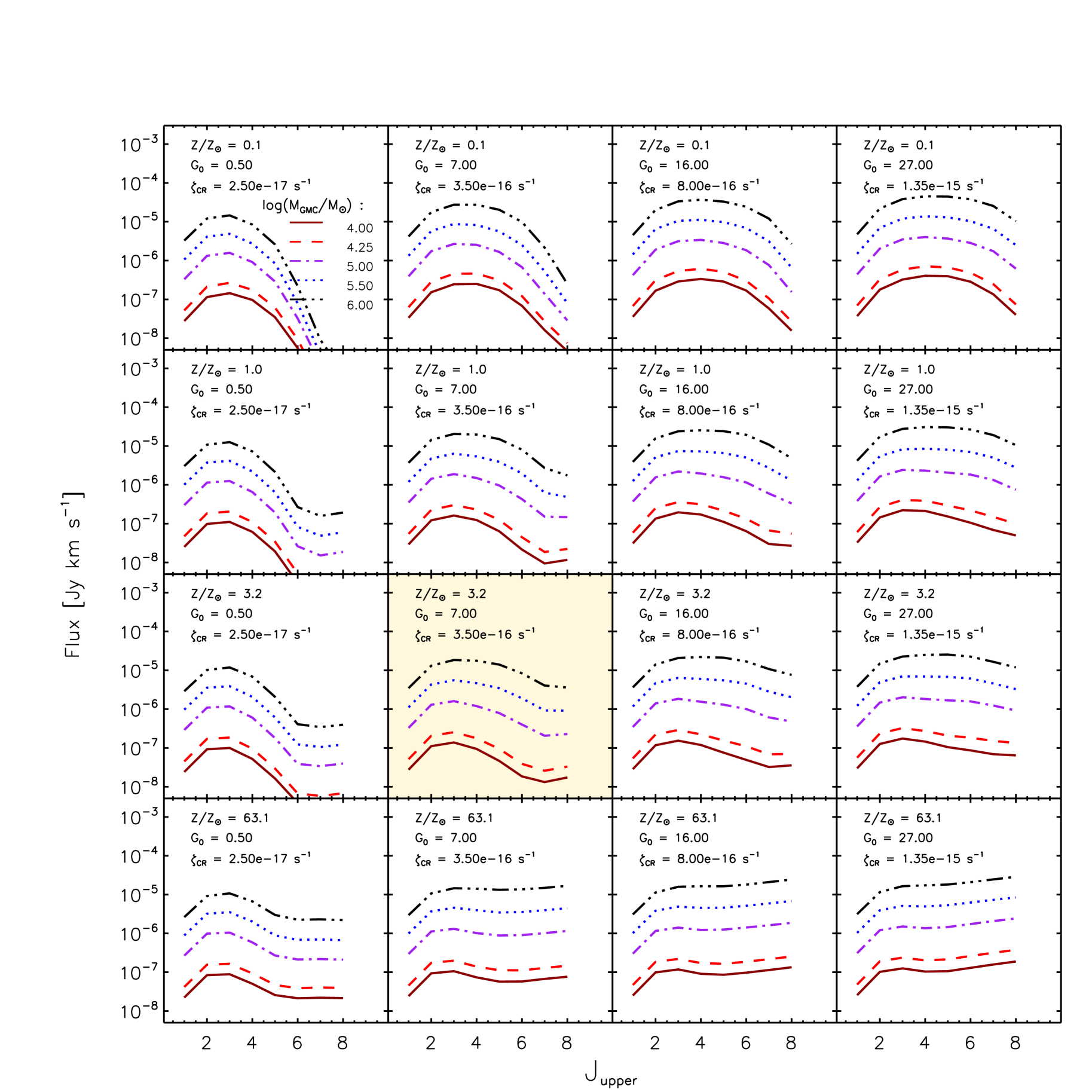
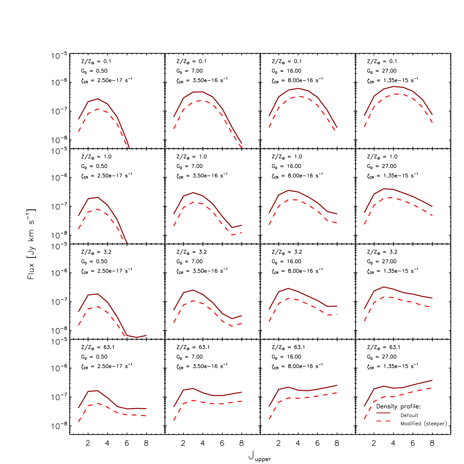
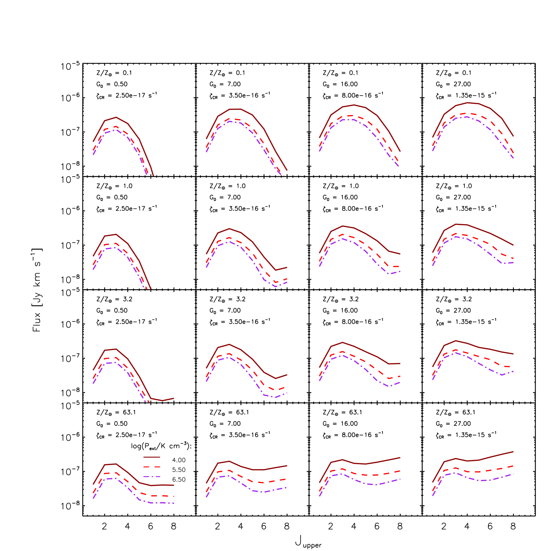
Appendix D Testing sígame on MW-like galaxies

As a benchmark test, sígame was applied to galaxy simulations at $z=0$ with properties similar to those of the MW. The reasoning here was that since much of the sub-grid physics adopted by sígame relies on empirical relations observed in the MW (e.g., the GMC mass spectrum index), the method ought to come close to re-producing the observed CO properties of spiral galaxies, such as our MW, in the local universe.

The three galaxies (hereafter denoted MW1, MW2, and MW3 in order of increasing SFR) were selected from a more recent version of the SPH simulation described in Section 2. The properties of MW1, MW2, and MW3 are listed in Table 5 and are seen to be within a factor $\sim 2-6$ of the stellar mass (${\rm M}_{*,\rm{MW}}=6\times 10^{10}$ $\rm{M}_{\odot}$; McMillan, 2011) and SFR ($1.9\pm 0.4$ $\rm{M}_{\odot}$ yr^-1; Chomiuk & Povich, 2011) of the MW.

The steps outlined in Section 3.1 (and further described in Sections 3.2 to 3.4.3) were followed, but with two minor modifications: 1) the CMB temperature at $z=0$ was set to 2.725 K rather than 8.175 K used at $z=2$, and 2) the resolved FUV fields of our MW-like model galaxies span a range below that seen in our $z=2$ model galaxies (cf. Figure 15) meaning that the $G_{0}^{\prime}$ parameter values for our GMC grid had to be adjusted correspondingly. The following $G_{0}^{\prime}$ grid points were chosen: $[0.05,0.1,0.15,0.1,0.2,0.4,0.6,0.8,1.0,1.2]$ Habing.

In Figure 20 we compare the resulting CO SLEDs with that of the MW from Fixsen et al. (1999), as well as with those of M 51 ($M_{\ast}=4.7\times 10^{10}\,\mbox{$\rm{M}_{\odot}$};$ Mentuch Cooper et al. (2012), ${\rm SFR}=2.6$ $\rm{M}_{\odot}$ yr^-1; Schuster et al. 2007) from Vlahakis et al. (2013), Hughes et al. (2013) and Kamenetzky et al. (2015), M 83 ($M_{\ast}=7.9\times 10^{10}\,\mbox{$\rm{M}_{\odot}$}$ and ${\rm SFR}=3.2$ $\rm{M}_{\odot}$ yr^-1; Jarrett et al. 2013) from Wu et al. (2015) and other local galaxies of IR luminosity within 20% of that of the MW ($1.8\times 10^{10}$ $L_{\odot}$; Wright et al. 1991) from Kamenetzky et al. (2015). M 51 is a nearby galaxy slightly smaller in size and stellar mass than the MW, whereas M 83 is more massive and star-forming than the MW. The dispersion in observed CO SLEDs among the MW, M 83, M 51 and other local galaxies, allows for a large range in normalization and shape of the CO SLED within which our model galaxies find themselves.

The CO line luminosities of the MW lie roughly in the range spanned by the CO SLEDs of MW2 and MW3 up to and including $J_{\rm up}=4$, but significantly above that of MW1. For the higher $J$ transitions the line luminosities of our simulations drop off more rapidly than the MW, meaning that our model galaxies have lower luminosities compared to the MW (and other local galaxies of IR luminosities within 20% from that of the MW; long-dashed orange lines) at $J_{\rm up}>4$. This suggests that our simulations are missing a warm/dense component which is required to significantly excite these high-$J$ lines. The agreement between the CO SLED of MW2 and that of M 51 is good at low transitions ($J_{\rm up}<6$), which is encouraging given that the two galaxies have nearly identical SFR and $M_{\ast}$. At higher $J$ values, the CO SLED of M 51 has an excess of CO emission when compared with MW2, corresponding to a warm gas phase not captured by our models. This warm phase is more pronounced in signature when looking at the CO SLED of M 83, the line ratios of which are above our model galaxies for all $J_{\rm up}>2$. Our models MW1, MW2 and MW3 only agree in CO luminosity with M 51 at the $J_{\rm up}=4$ and $5$ transitions.

As for brightness temperature ratios (see middle panel) of our simulated MW-like galaxies only agree with the MW within the observational errors at CO(4$-$3), and other wise display a CO SLED shape noticably different from the MW. Where our model galaxies peak at the CO(3$-$2) transition in velocity-integrated intensity (see bottom panel), similar to M 51, the MW and M 83 peak at CO(4$-$3). However, nowhere do the simulated line ratios differ by more than a factor of 2.

The molecular gas masses of MW1, MW2 and MW3 are $4.6$, $5.4$ and $8.5\times 10^{9}\,\mbox{$\rm{M}_{\odot}$}$, respectively, significantly above $(1.0\pm 0.3)\times 10^{9}\,\mbox{$\rm{M}_{\odot}$}$ for the MW (Heyer & Dame, 2015). The corresponding global ($R<20\,$kpc) $\alpha_{\rm CO}$ factors are $13.6$, $7.7$ and $7.0\,\mbox{$\rm{M}_{\odot}$}\,\rm{pc}^{-2}$ (K km s^-1)^-1. For the inner disk ($R<10\,\rm{kpc}$) of the MW, $\alpha_{\rm CO,MW}\simeq 4.3\pm 0.1\,{\rm\mbox{$\rm{M}_{\odot}$}\,pc^{-2}\,(K\,km\,s^{-1})^{-1}}$ (e.g., Strong & Mattox, 1996; Dame et al., 2001; Pineda et al., 2008; Bolatto et al., 2013). However, typically the measurements of $\alpha_{\rm CO}$ in the MW do not probe the central ($<1\,$kpc) region. Excluding the central $R<1\,$kpc region and going out to $R=10\,$kpc, the $\alpha_{\rm CO}$ factors of MW1, MW2 and MW3 are $11.6$, $6.9$ and $6.2\,\mbox{$\rm{M}_{\odot}$}\,\rm{pc}^{-2}$ (K km s^-1)^-1, i.e. factors of $2.7$, $1.6$ and $1.4$ above $\alpha_{\rm CO,MW}$, respectively.

Table 5: Properties of the three $z=0$ MW-like galaxies (MW1, MW2, and MW3) used to benchmark sígame.

	SFR	$M_{\ast}$	$M_{\rm SPH}$	$f_{\rm SPH}$	$Z^{\prime}$	$R_{\rm cut}$
	[$\rm{M}_{\odot}$ yr-1 ]	[$10^{10}$ $\rm{M}_{\odot}$ ]	[$10^{10}$ $\rm{M}_{\odot}$ ]			[kpc]
MW1	2.2	$0.97$	$1.17$	55%	2.07	$20$
MW2	4.1	$3.12$	$1.27$	29%	3.31	$20$
MW3	6.2	$3.83$	$1.69$	31%	3.90	$20$

Notes. All quantities are determined within a radius $R_{\rm cut}$, which is the radius where the cumulative radial stellar mass function of each galaxy becomes flat. The gas mass ($M_{\rm SPH}$) is the total SPH gas mass within $R_{\rm cut}$. The metallicity ($\mbox{$Z^{\prime}$}=Z/Z_{\odot}$) is the mean of all SPH gas particles within $R_{\rm cut}$.

Figure 20: Global CO SLEDs of our three model galaxies MW1, MW2 and MW3 shown as red (dashed), green (dash-dot) and blue (dash-dot-dot-dot) curves, respectively, selected to represent the MW in terms of stellar mass and SFR. The SLEDs are given as absolute line luminosities in units of K km s^-1  pc^-2 (top panel), as brightness temperature ratios normalised to the CO(1$-$0) transition (middle panel), and as velocity-integrated intensity ratios normalised to CO(1$-$0) (bottom panel). The observed global CO SLED of the MW is shown in grey (Fixsen et al., 1999), and global CO measurements of the local star-forming galaxy M 51 are displayed with triangles. The CO observations for M 51 are from Vlahakis et al. (2013) and Hughes et al. (2013). Also shown, with long-dashed orange lines, are observed CO SLEDs of local galaxies with IR luminosities within $20\%$ of that of the MW (Kamenetzky et al., 2015).

References

- Ackermann et al. (2013) Ackermann M., et al., 2013, Science, 339, 807
- Adelberger et al. (2004) Adelberger K. L., Steidel C. C., Shapley A. E., Hunt M. P., Erb D. K., Reddy N. A., Pettini M., 2004, ApJ, 607, 226
- Aravena et al. (2010) Aravena M., et al., 2010, ApJ, 718, 177
- Aravena et al. (2014) Aravena M., et al., 2014, MNRAS, 442, 558
- Asplund et al. (2009) Asplund M., Grevesse N., Sauval A. J., Scott P., 2009, ARA&A, 47, 481
- Bakes & Tielens (1994) Bakes E. L. O., Tielens A. G. G. M., 1994, ApJ, 427, 822
- Barvainis et al. (1994) Barvainis R., Tacconi L., Antonucci R., Alloin D., Coleman P., 1994, Nature, 371, 586
- Bigiel et al. (2008) Bigiel F., Leroy A., Walter F., Brinks E., de Blok W. J. G., Madore B., Thornley M. D., 2008, AJ, 136, 2846
- Black & Dalgarno (1977) Black J. H., Dalgarno A., 1977, ApJs, 34, 405
- Blanc et al. (2013) Blanc G. A., et al., 2013, ApJ, 764, 117
- Blitz & Rosolowsky (2006) Blitz L., Rosolowsky E., 2006, ApJ, 650, 933
- Blitz et al. (2007) Blitz L., Fukui Y., Kawamura A., Leroy A., Mizuno N., Rosolowsky E., 2007, Protostars and Planets V, pp 81–96
- Bolatto et al. (2008) Bolatto A. D., Leroy A. K., Rosolowsky E., Walter F., Blitz L., 2008, ApJ, 686, 948
- Bolatto et al. (2013) Bolatto A. D., Wolfire M., Leroy A. K., 2013, ARA&A, 51, 207
- Bothwell et al. (2013) Bothwell M. S., et al., 2013, ApJ, 779, 67
- Bovy et al. (2012) Bovy J., Rix H.-W., Hogg D. W., 2012, ApJ, 751, 131
- Brinch & Hogerheijde (2010) Brinch C., Hogerheijde M. R., 2010, A&A, 523, A25
- Bryant & Scoville (1999) Bryant P. M., Scoville N. Z., 1999, AJ, 117, 2632
- Carilli & Walter (2013) Carilli C. L., Walter F., 2013, ARAA, 51, 105
- Carroll & Goldsmith (1981) Carroll T. J., Goldsmith P. F., 1981, ApJ, 245, 891
- Cazaux & Spaans (2004) Cazaux S., Spaans M., 2004, ApJ, 611, 40
- Chabrier (2003) Chabrier G., 2003, PASP, 115, 763
- Chomiuk & Povich (2011) Chomiuk L., Povich M. S., 2011, AJ, 142, 197
- Christensen et al. (2012) Christensen C., Quinn T., Governato F., Stilp A., Shen S., Wadsley J., 2012, MNRAS, 425, 3058
- Daddi et al. (2004) Daddi E., Cimatti A., Renzini A., Fontana A., Mignoli M., Pozzetti L., Tozzi P., Zamorani G., 2004, ApJ, 617, 746
- Daddi et al. (2010) Daddi E., et al., 2010, ApJ, 713, 686
- Daddi et al. (2015) Daddi E., et al., 2015, A&A, 577, A46
- Dame et al. (2001) Dame T. M., Hartmann D., Thaddeus P., 2001, ApJ, 547, 792
- Dannerbauer et al. (2009) Dannerbauer H., Daddi E., Riechers D. A., Walter F., Carilli C. L., Dickinson M., Elbaz D., Morrison G. E., 2009, ApJL, 698, L178
- Downes & Solomon (1998) Downes D., Solomon P. M., 1998, ApJ, 507, 615
- Draine (2011) Draine B. T., 2011, Physics of the Interstellar and Intergalactic Medium. Princeton University Press
- Elmegreen (1989) Elmegreen B. G., 1989, ApJ, 344, 306
- Fixsen et al. (1999) Fixsen D. J., Bennett C. L., Mather J. C., 1999, ApJ, 526, 207
- Frayer et al. (1998) Frayer D. T., Ivison R. J., Scoville N. Z., Yun M., Evans A. S., Smail I., Blain A. W., Kneib J.-P., 1998, ApJL, 506, L7
- Geach & Papadopoulos (2012) Geach J. E., Papadopoulos P. P., 2012, ApJ, 757, 156
- Glover & Clark (2012) Glover S. C. O., Clark P. C., 2012, MNRAS, 421, 9
- Gnat & Sternberg (2007) Gnat O., Sternberg A., 2007, ApJS, 168, 213
- Goldsmith (2001) Goldsmith P. F., 2001, ApJ, 557, 736
- Greve & Sommer-Larsen (2008) Greve T. R., Sommer-Larsen J., 2008, A&A, 480, 335
- Haardt & Madau (2001) Haardt F., Madau P., 2001, preprint, (arXiv:astro-ph/0106018)
- Heiderman et al. (2010) Heiderman A., Evans II N. J., Allen L. E., Huard T., Heyer M., 2010, ApJ, 723, 1019
- Heyer & Brunt (2004) Heyer M. H., Brunt C. M., 2004, ApJL, 615, L45
- Heyer & Dame (2015) Heyer M., Dame T. M., 2015, ARA&A, 53, 583
- Hughes et al. (2013) Hughes A., et al., 2013, ApJ, 779, 44
- Iono et al. (2009) Iono D., et al., 2009, ApJ, 695, 1537
- Jarrett et al. (2013) Jarrett T. H., et al., 2013, AJ, 145, 6
- Kamenetzky et al. (2015) Kamenetzky J., Rangwala N., Glenn J., Maloney P. R., Conley A., 2015, preprint, (arXiv:1508.05102)
- Kennicutt (1998) Kennicutt Jr. R. C., 1998, ARA&A, 36, 189
- Krumholz & Gnedin (2011) Krumholz M. R., Gnedin N. Y., 2011, ApJ, 729, 36
- Krumholz et al. (2009) Krumholz M. R., McKee C. F., Tumlinson J., 2009, ApJ, 699, 850
- Lagos et al. (2012) Lagos C. d. P., Bayet E., Baugh C. M., Lacey C. G., Bell T. A., Fanidakis N., Geach J. E., 2012, MNRAS, 426, 2142
- Larson (1981) Larson R. B., 1981, MNRAS, 194, 809
- Lee et al. (1996) Lee H.-H., Bettens R. P. A., Herbst E., 1996, A&As, 119, 111
- Leroy et al. (2008) Leroy A. K., Walter F., Brinks E., Bigiel F., de Blok W. J. G., Madore B., Thornley M. D., 2008, AJ, 136, 2782
- Leroy et al. (2015) Leroy A. K., et al., 2015, ApJ, 801, 25
- Magnelli et al. (2012) Magnelli B., et al., 2012, A&A, 548, A22
- Mao et al. (2010) Mao R.-Q., Schulz A., Henkel C., Mauersberger R., Muders D., Dinh-V-Trung 2010, ApJ, 724, 1336
- McMillan (2011) McMillan P. J., 2011, MNRAS, 414, 2446
- Mentuch Cooper et al. (2012) Mentuch Cooper E., et al., 2012, ApJ, 755, 165
- Monaghan (2005) Monaghan J. J., 2005, Reports on Progress in Physics, 68, 1703
- Muñoz & Furlanetto (2013) Muñoz J. A., Furlanetto S. R., 2013, MNRAS, 435, 2676
- Narayanan & Hopkins (2013) Narayanan D., Hopkins P. F., 2013, MNRAS, 433, 1223
- Narayanan & Krumholz (2014) Narayanan D., Krumholz M. R., 2014, MNRAS, 442, 1411
- Narayanan et al. (2006) Narayanan D., et al., 2006, ApJL, 642, L107
- Narayanan et al. (2008a) Narayanan D., et al., 2008a, ApJS, 174, 13
- Narayanan et al. (2008b) Narayanan D., et al., 2008b, ApJs, 176, 331
- Narayanan et al. (2008c) Narayanan D., Cox T. J., Shirley Y., Davé R., Hernquist L., Walker C. K., 2008c, ApJ, 684, 996
- Narayanan et al. (2009) Narayanan D., Cox T. J., Hayward C. C., Younger J. D., Hernquist L., 2009, MNRAS, 400, 1919
- Narayanan et al. (2011) Narayanan D., Krumholz M., Ostriker E. C., Hernquist L., 2011, MNRAS, 418, 664
- Narayanan et al. (2012) Narayanan D., Krumholz M. R., Ostriker E. C., Hernquist L., 2012, MNRAS, 421, 3127
- Neri et al. (2003) Neri R., et al., 2003, ApJL, 597, L113
- Norman & Spaans (1997) Norman C. A., Spaans M., 1997, ApJ, 480, 145
- Obreschkow et al. (2009) Obreschkow D., Klöckner H.-R., Heywood I., Levrier F., Rawlings S., 2009, Apj, 703, 1890
- Obreschkow et al. (2011) Obreschkow D., Heywood I., Rawlings S., 2011, ApJ, 743, 84
- Pan & Padoan (2009) Pan L., Padoan P., 2009, ApJ, 692, 594
- Papadopoulos & Thi (2013) Papadopoulos P. P., Thi W.-F., 2013, in Torres D. F., Reimer O., eds, Advances in Solid State Physics Vol. 34, Cosmic Rays in Star-Forming Environments. Springer-Verlag, Berlin, Heidelberg, p. 41 (arXiv:1207.2048), doi:10.1007/978-3-642-35410-6˙5
- Papadopoulos et al. (2010) Papadopoulos P. P., Isaak K., van der Werf P., 2010, ApJ, 711, 757
- Papadopoulos et al. (2011) Papadopoulos P. P., Thi W.-F., Miniati F., Viti S., 2011, MNRAS, 414, 1705
- Papadopoulos et al. (2012) Papadopoulos P. P., van der Werf P. P., Xilouris E. M., Isaak K. G., Gao Y., Mühle S., 2012, MNRAS, 426, 2601
- Papadopoulos et al. (2014) Papadopoulos P. P., et al., 2014, ApJ, 788, 153
- Papovich et al. (2011) Papovich C., Finkelstein S. L., Ferguson H. C., Lotz J. M., Giavalisco M., 2011, MNRAS, 412, 1123
- Pelupessy (2005) Pelupessy F. I., 2005, PhD thesis, Leiden Observatory, Leiden University, P.O. Box 9513, 2300 RA Leiden, The Netherlands
- Pelupessy et al. (2006) Pelupessy F. I., Papadopoulos P. P., van der Werf P., 2006, ApJ, 645, 1024
- Pineda et al. (2008) Pineda J. E., Caselli P., Goodman A. A., 2008, ApJ, 679, 481
- Pineda et al. (2013) Pineda J. L., Langer W. D., Velusamy T., Goldsmith P. F., 2013, A&A, 554, A103
- Planck Collaboration XVI (2014) Planck Collaboration XVI 2014, A&A, 571, A16
- Plummer (1911) Plummer H. C., 1911, MNRAS, 71, 460
- Popping et al. (2014) Popping G., Pérez-Beaupuits J. P., Spaans M., Trager S. C., Somerville R. S., 2014, MNRAS, 444, 1301
- Price (2007) Price D. J., 2007, Publications of the Astronomical Society of Australia, 24, 159
- Puchwein et al. (2015) Puchwein E., Bolton J. S., Haehnelt M. G., Madau P., Becker G. D., Haardt F., 2015, MNRAS, 450, 4081
- Riechers et al. (2011) Riechers D. A., et al., 2011, ApJL, 739, L32
- Rodighiero et al. (2010) Rodighiero G., et al., 2010, A&A, 518, L25
- Röllig et al. (2006) Röllig M., Ossenkopf V., Jeyakumar S., Stutzki J., Sternberg A., 2006, A&A, 451, 917
- Romeo et al. (2006) Romeo A. D., Sommer-Larsen J., Portinari L., Antonuccio-Delogu V., 2006, MNRAS, 371, 548
- Saintonge et al. (2011) Saintonge A., et al., 2011, MNRAS, 415, 32
- Sandstrom et al. (2013) Sandstrom K. M., et al., 2013, ApJ, 777, 5
- Schöier et al. (2005) Schöier F. L., van der Tak F. F. S., van Dishoeck E. F., Black J. H., 2005, A&A, 432, 369
- Schuster et al. (2007) Schuster K. F., Kramer C., Hitschfeld M., Garcia-Burillo S., Mookerjea B., 2007, A&A, 461, 143
- Seon et al. (2011) Seon K.-I., et al., 2011, ApJs, 196, 15
- Simnett & McDonald (1969) Simnett G. M., McDonald F. B., 1969, ApJ, 157, 1435
- Smith et al. (2008) Smith B., Sigurdsson S., Abel T., 2008, MNRAS, 385, 1443
- Smith et al. (2014) Smith R. J., Glover S. C. O., Clark P. C., Klessen R. S., Springel V., 2014, MNRAS, 441, 1628
- Sofia et al. (2004) Sofia U. J., Lauroesch J. T., Meyer D. M., Cartledge S. I. B., 2004, ApJ, 605, 272
- Solomon et al. (1997) Solomon P. M., Downes D., Radford S. J. E., Barrett J. W., 1997, ApJ, 478, 144
- Sommer-Larsen et al. (1998) Sommer-Larsen J., Vedel H., Hellsten U., 1998, MNRAS, 294, 485
- Sommer-Larsen et al. (2003) Sommer-Larsen J., Götz M., Portinari L., 2003, ApJ, 596, 47
- Sommer-Larsen et al. (2005) Sommer-Larsen J., Romeo A. D., Portinari L., 2005, MNRAS, 357, 478
- Speagle et al. (2014) Speagle J. S., Steinhardt C. L., Capak P. L., Silverman J. D., 2014, ApJS, 214, 15
- Springel & Hernquist (2003) Springel V., Hernquist L., 2003, MNRAS, 339, 289
- Stahler & Palla (2005) Stahler S. W., Palla F., 2005, The Formation of Stars. Wiley
- Stinson et al. (2006) Stinson G., Seth A., Katz N., Wadsley J., Governato F., Quinn T., 2006, MNRAS, 373, 1074
- Strong & Mattox (1996) Strong A. W., Mattox J. R., 1996, A&A, 308, L21
- Swinbank et al. (2011) Swinbank A. M., et al., 2011, ApJ, 742, 11
- Tacconi et al. (2008) Tacconi L. J., et al., 2008, ApJ, 680, 246
- Tacconi et al. (2013) Tacconi L. J., et al., 2013, ApJ, 768, 74
- Tielens (2005) Tielens A. G. G. M., 2005, The Physics and Chemistry of the Interstellar Medium. Cambridge University Press
- Vlahakis et al. (2013) Vlahakis C., van der Werf P., Israel F. P., Tilanus R. P. J., 2013, MNRAS, 433, 1837
- Webber (1998) Webber W. R., 1998, ApJ, 506, 329
- Weiß et al. (2007) Weiß A., Downes D., Neri R., Walter F., Henkel C., Wilner D. J., Wagg J., Wiklind T., 2007, A&A, 467, 955
- Whitaker et al. (2011) Whitaker K. E., et al., 2011, ApJ, 735, 86
- Whitworth & Ward-Thompson (2001) Whitworth A. P., Ward-Thompson D., 2001, ApJ, 547, 317
- Wiersma et al. (2009) Wiersma R. P. C., Schaye J., Smith B. D., 2009, MNRAS, 393, 99
- Wolfire et al. (2003) Wolfire M. G., McKee C. F., Hollenbach D., Tielens A. G. G. M., 2003, ApJ, 587, 278
- Wolfire et al. (2010) Wolfire M. G., Hollenbach D., McKee C. F., 2010, ApJ, 716, 1191
- Wright et al. (1991) Wright E. L., et al., 1991, ApJ, 381, 200
- Wu et al. (2015) Wu R., et al., 2015, A&A, 575, A88
- Yang et al. (2010) Yang B., Stancil P. C., Balakrishnan N., Forrey R. C., 2010, ApJ, 718, 1062
- Yun et al. (2015) Yun M. S., et al., 2015, MNRAS, 454, 3485
- Zahid et al. (2012) Zahid H. J., Dima G. I., Kewley L. J., Erb D. K., Davé R., 2012, ApJ, 757, 54