Lines and continuum sky emission in the near infrared: observational constraints from deep high spectral resolution spectra with GIANO-TNG

Abstract

Aims. Determining the intensity of lines and continuum airglow emission in the H-band is important for the design of faint-object infrared spectrographs. Existing spectra at low/medium resolution cannot disentangle the true sky-continuum from instrumental effects (e.g. diffuse light in the wings of strong lines). We aim to obtain, for the first time, a high resolution infrared spectrum deep enough to set significant constraints on the continuum emission between the lines in the H-band.

Methods. During the second commissioning run of the GIANO high-resolution infrared spectrograph at the La Palma Observatory, we pointed the instrument directly to the sky and obtained a deep spectrum that extends from 0.97 to 2.4 $\mu$m.

Results. The spectrum shows about 1500 emission lines, a factor of two more than in previous works. Of these, 80% are identified as OH transitions; half of these are from highly excited molecules (hot-OH component) that are not included in the OH airglow emission models normally used for astronomical applications. The other lines are attributable to O₂ or unidentified. Several of the faint lines are in spectral regions that were previously believed to be free of line emission. The continuum in the H-band is marginally detected at a level of about 300 photons/m²/s/arcsec²/$\mu$m, equivalent to 20.1 AB-mag/arcsec². The observed spectrum and the list of observed sky-lines are published in electronic format.

Conclusions. Our measurements indicate that the sky continuum in the H-band could be even darker than previously believed. However, the myriad of airglow emission lines severely limits the spectral ranges where very low background can be effectively achieved with low/medium resolution spectrographs. We identify a few spectral bands that could still remain quite dark at the resolving power foreseen for VLT-MOONS (R$\simeq$6,600).

1 Introduction

The sky emission spectrum at infrared wavelengths and up to 1.8 $\mu$m (Y, J, H bands) is dominated by lines (airglow) emitted by OH and O₂ molecules; see e.g. Sharma Sharma (1985). These lines are intrinsically very narrow and, when observed at a high enough spectral resolution, they occupy only a small fraction of the spectrum. Therefore, by filtering the lines out, one could in principle decrease the sky background by orders of magnitudes, down to the level set by the sky continuum emission in between the lines. This apparently simple idea, often reported as ”OH sky-suppression”, has fostered a long and active field of research; see e.g. Oliva & Origlia Oliva92 (1992), Maihara et al. Maihara93 (1993), Herbst Herbst94 (1994), Content Content96 (1996), Ennico et al. Ennico98 (1998), Cuby et al. cuby00 (2000), Rousselot et al. Rousselot00 (2000), Iwamuro et al. Iwamuro01 (2001), Bland-Hawthorn et al. blandhawthorn04 (2004), Iwamuro et al. Iwamuro06 (2006), Ellis et al. ellis12 (2012), Trinh et al. Trinh13 (2013). However, in spite of the intense work devoted to measuring and modelling the properties of the sky spectrum, it is still not clear what is the real level of the sky continuum in between the airglow lines in the H-band (1.5-1.8 $\mu$m).

A detailed study of the infrared sky continuum emission was recently reported by Sullivan & Simcoe Sullivan (2012). Using spectra at a resolving power R=6,000 they were able to correct the spectra for all instrumental effects and derive accurate measurements of the sky continuum at wavelengths shorter than 1.3 $\mu$m (Y, J bands). However, they could not obtain precise results in the H-band (1.5-1.8 $\mu$m) because the sky continuum is well below the light diffused in the instrumental wings of the airglow lines. This problem was already noted in earlier works. In particular, Bland-Hawthorn et al. blandhawthorn04 (2004) claimed that the continuum level between the OH lines could be as low as the zodiacal light level and much lower than that measurable with classical (i.e. not properly OH suppressed) spectrographs. This claim was later retracted by Ellis et al. ellis12 (2012) after measuring the interline continuum with an optimised OH-suppression device based on a Bragg fibre grating. Trinh et al. Trinh13 (2013) subsequently attempted to model the interline continuum based on spectral models and measurements that did not reach the depth and completeness of the data presented in this paper.

The net - and somewhat surprising - result is that so far nobody has been able to improve the earliest measurements of Maihara et al. Maihara93 (1993) who reported a continuum emission of 590 photons/m²/s/arcsec²/$\mu$m measured at 1.665 $\mu$m (equivalent to 19.4 AB-mag/arcsec²) using a spectrometer with resolving power R=17,000. equipped with one of the first-generation 256² HgCdTe infrared detectors

A proper understanding of the line and continuum emission from the sky is of fundamental importance when designing new infrared spectrographs optimised for observations of very faint targets. A representative case is that of MOONS, the multi-objects optical and near infrared spectrometer for the VLT, see Cirasuolo et al. (cirasuolo11 (2011), cirasuolo14 (2014)). This instrument includes an arm covering the H-band at a resolving power R$\simeq$6,600. The requirements on instrumental background and stray light strongly depend on the sky continuum one assumes, see Li Causi et al. licausi (2014) for details.

In a previous work (Oliva et al. paper1 (2013)) we presented, for the first time, observations of the infrared sky spectrum at high spectral resolution and covering a very wide spectral range. The spectrum revealed 750 emission lines, many of these never reported before. However, the data were not deep enough to provide significant constraints on the continuum emission in between the lines.

Here we present and discuss new measurements taken with GIANO during the second commissioning run at Telescopio Nazionale Galileo (TNG). In Sect. 2 we briefly describe the instrument, the measurements, and the data reduction. In Sects. 3 and 4 we present and discuss the results.

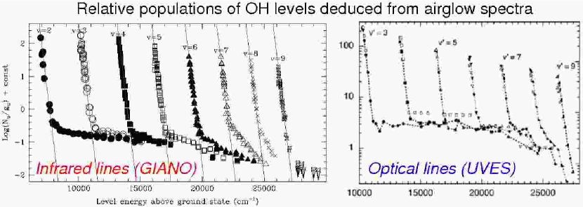
Figure 1: Derived column densities of the OH levels plotted against the energy of the levels above the ground-state of the molecule. The left panel shows the values derived from the infrared lines discussed here while the right hand panel – reproduced under permission from Fig. 16 of Cosby & Slanger Cosby (2007); © Canadian Science Publishing or its licensors – summarizes the results based on optical (UVES) spectra. The steep straight lines in the left panel show the distribution predicted by standard models with rotational levels thermalised at 200 K. The quasi-flat tails reveal the hot-OH component, see Sect. 3.1 for details.

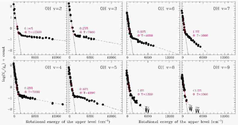
Figure 2: Same as Fig. 1 but with separate panels for each vibrational level. The straight solid lines represent the cold-OH component while the dashed curves show the distribution obtained adding a fraction of hot-OH molecules. The numerical fraction and rotational temperature of the hot-OH molecules is reported within each panel. See text, Sect 3.1 for details.

2 Observations and spectral analysis

GIANO is a cross-dispersed cryogenic spectrometer that simultaneously covers the spectral range from 0.97 $\mu$m to 2.4 $\mu$m with a maximum resolving power of R$\simeq$50,000 for a 2-pixels slit. The main disperser is a commercial R2 echelle grating with 23.2 lines/mm that works on a $\oslash$100 mm collimated beam. Cross dispersion is performed by prisms (one made of fused silica and two made of ZnSe) that work in double pass. The prisms cross-disperse the light both before and after it is dispersed by the echelle gratings; this setup produces a curvature of the images of the spectral orders. The detector is a HgCdTe Hawaii-II-PACE with 2048² pixels. Its control system is extremely stable with a remarkably low read-out noise (see Oliva et al.  2012b ). More technical details on the instrument can be found in Oliva et al.  2012a and references therein.

GIANO was designed and built for direct light feeding from the TNG 3.5 m telescope. Unfortunately, the focal station originally reserved was not available when GIANO was commissioned. Therefore we were forced to position the spectrograph on the rotating building and develop a complex light-feed system using a pair of IR-transmitting ZBLAN fibres with two separate opto-mechanical interfaces. The first interface is used to feed the telescope light into the fibres; it also includes the guiding camera and the calibration unit. The second interface re-images the light from the fibres onto the cryogenic slit; see Tozzi et al. tozzi14 (2014) for more details.

The overall performances of GIANO are negatively affected by the complexity of the interfaces and by problems intrinsic to the fibres: the efficiency has been lowered by almost a factor of 3 and the spectra are affected by modal-noise, especially at longer wavelengths. Consequently, the observations of the sky taken during normal operations are not appropriate to reveal the faintest airglow lines and the continuum emission in between. To overcome this problem we took advantage of the early part of a test night (September 3, 2014) to secure a direct spectrum of the sky with GIANO. We moved the spectrograph to the main entrance of the TNG and arranged a simple pre-slit system (a lens doublet and two flat mirrors) to feed the cryogenic slit with the light from a sky-area in the ESE quadrant at a zenith distance of about 25 degrees. The half moon was in the SSW quadrant at a zenith distance of 50 degrees.

We integrated the sky for two hours using the 3-pixels slit that is normally used in combination with the fibre interface. This yields a resolving power R$\simeq$32,000. For calibration we took several long series of darks interspaced with flat frames. This strategy was chosen because the sky spectra showed some residuals (persistency) of a flat frame taken many hours before. We therefore re-created different pseudo-darks with different levels of persistency and, during the reduction, we selected the combination of pseudo-darks that best reproduced the persistency pattern. The criterion for selection relied on the assumption that the sky continuum emission is zero in the spectral regions were the atmosphere is opaque, i.e. in the 1.37-1.40 $\mu$m range (orders 54-56 of the GIANO echellogram). In other words, we took advantage of the fact that the flat and its residual persistency have similar intensities over the full spectral range, while the spectrum of any light source above the troposphere (i.e. astronomical targets and the sky airglow emission) is absorbed by the water bands.

The acquisitions were performed using the standard setup of the controller, i.e. on chip integrations of 5 minutes with multiple non-destructive read-outs every 10 seconds. All the read-outs were separately stored. The ”ramped-frames” were constructed later-on using the algorithm described in Oliva et al. 2012b that, besides applying the standard Fowler sampling, it also minimises the effects of reset-anomaly and cosmic rays.

The 1D spectra were extracted by summing 20 pixels along the slit. Wavelength calibration was performed using U-Ne lamp frames taken after the series of darks. The spectrometer is stable to $<$0.1 pixels (i.e. $\Delta\lambda/\lambda\!<\!10^{-6}$ r.m.s.). The wavelengths of the uranium lines were taken from Redman et al. redman2011 (2011), while for neon we used the table available on the NIST website. The resulting wavelength accuracy was about 0.07 Å r.m.s. for lines in the H-band.

The flat exposures were used to determine and correct the variation of instrumental efficiency within each order. An approximate flux calibration was performed by assuming that the relative efficiencies of the orders are the same as when observing standard stars through the fibre-interface and the TNG telescope. This is a very reasonable assumption within the relatively narrow wavelength range covered by the H-band. However, it may cause systematic errors (up to 0.3 dex) in the relative fluxes of lines with very different wavelengths. Absolute flux calibration was roughly estimated by imposing that the flux of the OH [4-0]Q1(1.5) line at 1.5833 $\mu$m is 270 photons/m²/s/arcsec²; i.e. the typical value measured during normal observing nights.

3 The sky lines and continuum emission

A total of about 1500 airglow lines were detected in the spectrum. Compared to Paper 1, we have doubled the number of emission features measured. In the following we separately discuss the OH lines, the other emission features and the continuum emission in the Y, J, and H bands.

3.1 OH lines and the hot-OH component

Table 1 (available only in electronic format) lists the lines identified as OH transitions. For each $\Lambda$-doublet we give the wavelengths (in vacuum) and the total observed flux of the doublet, normalised to the brightest transition. For the fluxes we assumed that the two components of each doublet have equal intensities, i.e. that the ’$e$’ and ’$f$’ sub-levels are in thermal equilibrium; this is appropriate for the density and temperature of the mesosphere. The listed wavelengths are derived from the newest OH molecular constants by Bernath & Colin Bernath (2009). These include highly excited rotational states and allowed us to identify OH lines from rotational levels as high as J=22.5, thus adding important constraints on the hot component of OH emission. This component was already reported by Cosby & Slanger Cosby (2007) and in Paper 1. It is not included in any of the models of OH airglow emission normally used for astronomical applications. These assume that the OH molecules have a very high vibrational temperature ($T_{vib}\simeq 9000$ K) and a much lower rotational temperature ($T_{rot}\simeq 200$ K). In other words they assume that the gas density is high enough to make collisional transitions between rotational states much faster than radiative de-excitations. This brings the rotational temperature to values similar to the kinetic temperature of the gas. The net result is that all the lines from levels with rotational quantum number J$>$8.5 are normally predicted to be extremely faint and totally negligible. The number of lines that are missed by standard models can be directly visualised in Fig. 1 that plots the column densities of the upper levels of the measured lines as a function of the excitation energy of the levels. The steep lines show the distribution expected for a single gas component with rotational levels thermalised at T=200 K. The points in the quasi-flat tails represent emission lines from hot molecules that are not thermalised. According to Cosby & Slanger Cosby (2007), this hot component is related to low density clouds at higher altitudes. Here the gas density is lower than the critical density of the rotational levels and, therefore, the population of the levels remain similar to that set at the moment the OH molecule is formed.

In order to provide a practical tool to predict the intensities of all OH lines we have fitted the observed level distribution with a mixture of two components. The first is the standard model (cold-OH), while the second (hot-OH) has a rotational temperature that is empirically determined from the observed values. Each vibrational state must be separately fit to obtain a good matching. This simple model works as follows: let $N_{u}$ (cm^-2) be the column density of a given state ($v,J,F$) of the OH molecule. This quantity is related to the excitation temperatures by the standard Boltzmann equations, i.e.

$${N_{u}\over g_{u}N_{OH}}=e^{-E_{v}/kT_{v}}\ \ \left[\eta_{rc}{e^{-E_{J,F}/kT_{rc}}\over U(T_{v},T_{rc})}+\eta_{rh}{e^{-E_{J,F}/kT_{rh}}\over U(T_{v},T_{rh})}\right]$$

where $g_{u}$ is statistical weight of the level, $N_{OH}$ is the total column density of OH molecules, $E_{v}$ is the vibrational energy of the level, $T_{v}$ is the vibrational temperature, $E_{J,F}$ is the rotational energy of the level, $T_{rc}$ is the rotational temperature of the cold component, $\eta_{rc}$ is the fraction of cold molecules, $T_{rh}$ is the rotational temperature of the hot component, $\eta_{rh}$ is the fraction of hot molecules and $U(T_{v},T_{r})$ is the partition function. The photon-flux of a given transition arising from the same level is given by

$$I_{ul}=N_{u}\cdot A_{ul}$$

where $A_{ul}$ (s^-1) is the transition probability. The points in Figs. 1, 2 are computed from Eq. (2) using the observed line intensities together with the molecular parameters of Bernath & Colin Bernath (2009) and the transition probabilities of van der Loo & Groenenboom vanderloo (2007). The steep straight lines in the left panel of Fig.  1 plot the function defined in Eq. (1) for $T_{v}$=9000 K, $T_{rc}$=200 K and $\eta_{rc}$=1 (i.e. only cold-OH). The same function is displayed in Fig.  2 where the dashed curves show the results obtained adding a hot-OH component with parameters ($\eta_{rh}$,$T_{rh}$) adjusted for each vibrational level; the values of the parameters are indicated in each panel.

The hot-OH component is most prominent in the lowest vibrational state (v=2) and becomes progressively weaker and cooler going to higher vibrational states; it virtually disappears at v=9.

3.2 O₂ and unidentified lines

The lines that cannot be associated with OH transitions are listed in Table 2 (this table is available only in electronic format). For the identification of the O₂ lines we used the HITRAN database (Rothman et al. hitran (2009)). Most of the identified transitions were already reported in Paper 1. A comparison between the two spectra shows that the intensity ratio between O₂ and OH lines has varied by almost a factor of 2 between the two epochs. This is not surprising: the Oxygen lines are known to vary by large factors even on timescales of hours. In our case the variation can be used to select those features that follow the time-behaviour of the O₂ lines. These lines are identified as “O2?” (i.e. probably O₂) in Table 2.

The remaining features are not identified. Of these 34 lines are closely spaced doublets with equal intensities. A representative example are the lines at $\lambda\lambda$17164.5, 17165.5 Å visible in the lower-right panel of Fig. 3. Several of these features were already detected in Paper 1. They are very similar to other $\Lambda$-split OH doublets detected in our spectra. However, their wavelengths do not correspond to any OH transition with $J_{u}\leq 40.5$ and $v_{u}\leq 10$. The possibility that these doublets are produced by OH isotopologues (e.g. ¹⁸OH) should be investigated, but is beyond the aims of this paper.

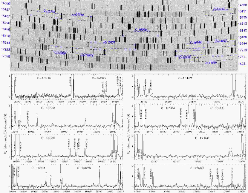
Figure 3: Upper panel: GIANO echelle spectrum of the H atmospheric band. Lower panels: extracted spectra in regions relatively free of line emission. The horizontal dashed lines show the level of 300 photons/m²/s/arcsec²/$\mu$m (equivalent to 20.1 AB-mag/arcsec²).

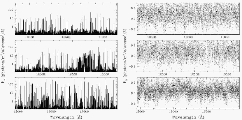
Figure 4: Left-hand panel: overview of the GIANO spectrum of the airglow. Right-hand panel: downscale to low flux levels. The spectral measurements are shown as separate dots to avoid confusion. The horizontal dashed line in the lowest panel shows the level of 300 photons/m²/s/arcsec²/$\mu$m (equivalent to 20.1 AB-mag/arcsec²).

Table 3: Spectral bands with low contamination from lines

Band	$\lambda$-range (Å)	$\Delta\lambda/\lambda$	Lines Flux
C-15167	15153 – 15183	0.0020	0.6 (210 ; 20.5)
C-15215	15195 – 15235	0.0026	–
C-15265	15245 – 15285	0.0026	1.6 (400 ; 19.8)
C-16000	15980 – 16020	0.0025	1.2 (320 ; 20.0)
C-16650	16620 – 16680	0.0036	2.3 (380 ; 19.9)
C-16784	16770 – 16798	0.0017	0.5 (170 ; 20.7)
C-16822	16808 – 16836	0.0017	–
C-16934	16918 – 16950	0.0019	1.3 (390 ; 19.8)
C-16976	16962 – 16990	0.0016	1.0 (360 ; 19.9)
C-17152	17134 – 17170	0.0021	0.7 (190 ; 20.6)
C-17580	17555 – 17605	0.0028	2.2 (430 ; 19.7)

3.3 The sky continuum emission

Within the H-band (1.5–1.8 $\mu$m) we detected:

• 514 lines of OH, half of which are produced by the hot-OH component described in Sect. 3.1;

• 41 lines of O₂, including two broad and prominent band-heads;

• 79 unidentified features.

Finding spectral regions free of emission features and far from bright airglow lines is already difficult in our spectra. It becomes virtually impossible at the lower resolving powers foreseen for MOONS (R$\simeq$6,600) and other faint-object IR spectrometers. In Fig. 3 we show the observed 2D echellogram of GIANO and the extracted 1D spectra of selected regions with relatively low contamination from lines. Their main parameters are listed in Table 3. They were selected with the following criteria:

• The width of the band must correspond to at least 10 resolution elements of MOONS (i.e. $\Delta\lambda/\lambda\!>\!1/660$)

• The band must include only faint lines whose total flux, averaged over the band-width, is less than 500 photons/m²/s/arcsec²/$\mu$m (equivalent to 19.6 AB-mag/arcsec²).

The broadest band is C-16650. It coincides with the region used by Maihara et al. Maihara93 (1993) to measure an average sky-continuum of 590 photons/m²/s/arcsec²/$\mu$m (equivalent to 19.4 AB-mag/arcsec²). We find that about 65% of this flux can be ascribed to five emission features (4 lines from hot-OH and one unidentified, see Fig. 3) that lie close to the centre of this band. Taken at face value, this would imply that the true continuum is $\simeq$200 photons/m²/s/arcsec²/$\mu$m (equivalent to 20.6 AB-mag/arcsec²). However, this number is affected by large uncertainties intrinsic to the procedure used to extract/average the continuum level from the spectrum and to variations of the sky lines between different epochs. Indeed, to reach a more reliable conclusion one would should re-analyse the raw data of Maihara et al. Maihara93 (1993) and correct them for the contribution of the sky-emission lines before computing the continuum level.

We attempted to measure the sky continuum emission using the extracted GIANO spectrum. This spectrum is shown in Fig. 4 and listed in Table 4 (available only in electronic format). The H-band has enough S/N ratio to show a faint continuum of about 300 photons/m²/s/arcsec²/$\mu$m (equivalent to 20.1 AB-mag/arcsec²); this level is shown as a dashed line in the figure. It corresponds to 5 e^-/pixel/hr at the GIANO detector. A formal computation of noise (i.e. including read-out, dark-current and photon statistics) yields a convincing 5$\sigma$ detection once the spectrum is re-sampled to a resolving power of R=5,000. The contribution by systematic errors is more difficult to estimate. On the one hand, the procedure used to subtract detector dark and persistency (see Sect. 2) has correctly produced a zero continuum in the bands where the atmosphere is opaque (the uppermost order in the 2D frame of Fig. 3). On the other hand, however, we cannot exclude that second order effects have left some residual instrumental artifacts in the H-band. An analysis of the dark frames affected by persistency indicates that second order effects tend to increase the residuals, rather than over-subtracting the residual continuum level in the H-band. Therefore, we are reasonably confident that the true sky-continuum cannot be larger than the observed value.

In the Y and J bands our spectra have a lower S/N ratio because the efficiency of the GIANO detector drops at shorter wavelengths. The measured upper limits correspond to about 19 AB-mag/arcsec² and are compatible with the measurements by Sullivan & Simcoe Sullivan (2012). In general, the Y and J bands are much less contaminated by line emission and the higher resolving power of GIANO is no longer needed to find spectral regions that properly sample the sky continuum.

4 Discussion and conclusions

We took advantage of the second commissioning of the GIANO high-resolution infrared spectrograph at La Palma Observatory to point the instrument directly to the sky. This yielded a sky spectrum much deeper than those collected through the fibre-interface to the TNG telescope and published in Oliva et al. paper1 (2013). The spectrum extends from 0.97 to 2.4 $\mu$m and includes the whole Y, J, and H-bands.

The spectrum shows about 1500 emission lines, a factor of two more than in previous works. Of these, 80% are identified as OH transitions while the others are attributable to O₂ or unidentified. Roughly half of the OH lines arise from highly excited rotational states, presumably associated with lower density clouds at higher altitudes. We derive physical parameters useful to model this hot-OH component that as yet has never been included in the airglow models used by astronomers.

Several of the faint lines are in spectral regions that were previously believed to be free of lines emission. The continuum in the H-band is marginally detected at a level of about 300 photons/m²/s/arcsec²/$\mu$m equivalent to 20.1 AB-mag/arcsec². In spite of the very low sky-continuum level, the myriad of airglow emission lines in the H-band severely limits the spectral ranges that can be properly exploited for deep observations of faint objects with low/medium resolution spectrographs. We have identified a few spectral bands that could still remain quite dark at the resolving power foreseen for the faint-object spectrograph VLT-MOONS (R=6,600).

The spectrum and the updated lists of observed infrared sky-lines are published in electronic format.

- (1) Bernath, P. F., & Colin, R. 2009, J. Mol. Spec., 257, 20
- (2) Bland-Hawthorn, J., Englund, M., & Edvell, G. 2004, Optics Express, 12, 5902
- (3) Cirasuolo, M., Afonso, J., Bender, et al. 2011, The Messenger, 145, 11
- (4) Cirasuolo, M., Afonso, J., Carollo, M., et al. 2014, SPIE, 9147E, 0N1
- (5) Content, R. 1996, ApJ, 464, 412
- (6) Cosby, P. C., & Slanger, T. G. 2007, Can. J. Phys., 85, 77
- (7) Cuby, J. G., Lidman, C., & Moutou, C. 2000, Messenger, 101, 2
- (8) Ellis, S. C., Bland-Hawthorn, J., Lawrence, J., et al. 2012, MNRAS, 425, 1682
- (9) Ennico, K. A., Parry, I. R., Kenworthy, M. A., et al. 1998, SPIE, 3354, 668
- (10) Herbst, T. M. 1994, PASP, 106, 1298
- (11) Iwamuro, F., Motohara, K., Maihara, T., Hata, R., & Harashima, T. 2001, PASJ, 53, 355
- (12) Iwamuro, F., Maihara, T., Ohta, K., et al. 2006, SPIE, 6269, 1B1
- (13) Li Causi, G., Cabral, A., Ferruzzi, D., et al. 2014 SPIE, 9147E, 641
- (14) Maihara, T., Iwamuro, F., Yamashita, T., et al. 1993, PASP, 105, 940
- (15) Oliva, E., & Origlia, L. 1992, A&A, 254, 466
- (16) Oliva, E., Origlia, L., Maiolino, R., et al. 2012a, SPIE, 8446, 3T1
- (17) Oliva, E., Biliotti, V., Baffa, C., et al. 2012b, SPIE, 8453, 2T1
- (18) Oliva, E., Origlia, L., Maiolino, R., et al. 2013, A&A, 555, A78
- (19) Redman, S. L., Lawler, J. E., Nave, G., Ramsey, L. W., & Mahadevan, S. 2011, ApJS, 195, 24
- (20) Rothman, L. S., Gordon, I. E., Barbe, A., et al. 2009, JQS&RT, 110, 533
- (21) Rousselot, P., Lidman, C., Cuby, J.-G., Moreels , G., & Monnet, G. 2000, A&A, 354, 1134
- (22) Sharma, R. D. 1985, Handbook of Geophysics, chapter 13 (Air Force Geophysics Laboratory, USAF)
- (23) Sullivan, P. W., & Simcoe, R. A. 2012, PASP, 124, 1336
- (24) Tozzi, A., Oliva, E., Origlia, L., et al. 2014, SPIE, 9147E, 9N1
- (25) Trinh, C. Q., Ellis, S. C., Bland-Hawthorn, J., et al. 2013, MNRAS, 432, 3262
- (26) van der Loo, M. P. J., & Groenenboom, G. C. 2007, J. of Chemical Physics, 126, 114314