Data Reduction with the MIKE Spectrometer

Rebecca A. Bernstein¹¹affiliation: Observatories of the Carnegie Institution for Science, 813 Santa Barbara Street, Pasadena, CA 91101, USA , Scott M. Burles²²affiliation: Cutler Group, LP, 101 Montgomery St. #700, SF, CA 94104 , J. Xavier Prochaska³³affiliation: Department of Astronomy and Astrophysics, UCO/Lick Observatory, University of California, 1156 High Street, Santa Cruz, CA 95064, USA

Abstract

This manuscript describes the design, usage, and data-reduction pipeline developed for the Magellan Inamori Kyocera Echelle (MIKE) spectrometer used with the Magellan telescope at the Las Campanas Observatory. We summarize the basic characteristics of the instrument and discuss observational procedures recommended for calibrating the standard data products. We detail the design and implementation of an IDL based data-reduction pipeline for MIKE data (since generalized to other echelle spectrometers, e.g. Keck/HIRES, VLT/UVES). This includes novel techniques for flat-fielding, wavelength calibration, and the extraction of echelle spectroscopy. Sufficient detail is provided in this manuscript to enable inexperienced observers to understand the strengths and weaknesses of the instrument and software package and an assessment of the related systematics.

Subject headings:

instrumentation : spectrographs – methods: data analysis – techniques: spectroscopic

1. Introduction

The field of astronomy has witnessed rapid growth over the past few decades leading to the division of astronomers into observers, instrumentationalists, and theorists. In recent years, there is even an increased specialization within these sub-classes (e.g. numericists vs. semi-analytic theorists, spectroscopy vs. adaptive optics imaging). Similarly, as observatories approach billion dollar projects the complexity of building a facility-class instruments exceeds the capacity of a single astronomer. In contrast to the recent past, it is impractical for the majority of observational astronomers to design and fabricate a new instrument as the most efficient means of pursuing his/her scientific interests.

Instead, modern observers now acquire and analyze data-sets without having even visited the telescope or even having developed intimate knowledge of the instrument. Furthermore, many observers now rely on data reduction pipelines to produce calibrated, science-quality data without a comprehensive knowledge of the trade-offs and limitations considered by the software designer(s). Although this trend toward virtual observing may improve the efficiency with which new data is obtained and analyzed, users of these tools are prone to having an incomplete understanding of his/her experiment.

Motivated by these trends, we have written the following paper to document the design, usage, and data reduction pipeline of the MIKE echelle spectrometer (Bernstein et al., 2003). We discuss observational techniques for the calibration of these data, new algorithms to improve sky subtraction and flat fielding, and object extraction. Although we focus on the MIKE spectrometer, we will give a pedagogical discussion that generalizes to the majority of echelle spectrometers in use today and in the future (e.g. HIRES, UVES; Vogt et al., 1994; Dekker et al., 2000). Portions of this manuscript also generalize to many of the low dispersion spectrometers in use today (e.g. DEIMOS, FORS, IMACS).

The principal goal of this paper is to describe the data reduction pipeline designed for the MIKE spectrometer and then generalized to the HIRES¹¹1http://www.ucolick.org/ $\sim$ xavier/HIRedux, UVES (e.g. Ellison, Prochaska & Lopez, 2007) and ESI²²2http://www2.keck.hawaii.edu/inst/esi/ESIRedux/ spectrometers within the XIDL package³³3http://www.ucolick.org/ $\sim$ xavier/IDL/index.html maintained by JXP. Many of the techniques we have implemented follow the standard lore of astronomical research, and we have benefited from many previous works on this topic (e.g. Churchill & Allen, 1995; Kelson, 2003). Furthermore, our efforts have been inspired by (and take advantage of) the algorithms developed for the spectral reductions of the Sloan Digital Sky Survey (SDSS; Burles & Schlegel, in prep.). Several unique characteristics of the MIKE spectrometer (e.g. tilted sky lines), however, have inspired new techniques for wavelength calibration, flat fielding, and object extraction. We describe these in detail in this manuscript; they may be of interest to future instruments where similar issues arise (e.g. X-shooter; D’Odorico et al., 2006).

The paper is organized as follows. In §2, we describe the MIKE double echelle briefly and highlight points which directly influence the design and implementation of the reduction algorithms described in this paper. In §3, we describe the layout of the software pipeline. In §4, we describe the image processing algorithms. In §5, we describe the flat field algorithms. In §6, we describe the wavelength calibration algorithms. In §7, we describe object tracing and extraction. Finally, we describe fluxing and coaddition algorithms in § 8.

2. Description of the Instrument

MIKE is a double echelle spectrograph which was designed for the Magellan telescopes and installed on Magellan II (Clay) during November 2002. The standard configuration for MIKE is set by the cross-over wavelength of the dichroic (originally at 4550Å and now 4950Å) and delivers complete wavelength coverage from 3350–5000 Å (blue) and 4900–9500 Å (red). The range can be adjusted down to $\sim 3200$ Å and up to $\sim 10,000$ Å on the red and blue sides, respectively.

In order to understand the strategies employed for observing and for data reduction, it is important to review the basic aspects of the optical and mechanical design of the instrument. We summarize these below and refer the reader to Bernstein et al. (2003) and the MIKE user guide for a more complete description (http://www.lco.cl).

The first optical element in MIKE beyond the slit is the dichroic window. The dichroic coating on the first surface reflects blue light and transmits red. After the dichroic, the two arms are independent but comprised of a similar train of optical elements. The beam on both sides is first converted from the F/11 focal ratio of the telescope to a roughly F/3.5 beam by a set of “injection” optics which essentially form a virtual image of the slit in the plane of each camera, offset from the CCD. A single set of large lenses then comprise the collimator/camera of each arm. These are used in double pass to first collimate the beam on its way to the dispersion elements, and then to focus the beam on its way back to the CCD. The gratings are used in quasi–littrow so that this virtual image of the slit and the echelle footprint are offset from each other in the focal plane of the camera/collimator. Between the camera/collimators and the gratings, both beams pass twice through a single prism on the red side and a pair of prisms on the blue side for cross dispersion.

Table 1Basic Parameters

	Blue Side	Red Side
focal ratio (effective)	F/3.9	F/3.6
scale at CCD	8.2 pix/^′′ ( $0.12^{\prime\prime}/$ pix)	7.5 pix/^′′ ( $0.13^{\prime\prime}/$ pix)
$\Delta\lambda$ /pixel (unbinned)	$\sim 0.02$ Å	$\sim 0.05$ Å
detector	$2048\times 4096$ (15 $\mu$ m pixels)	$2048\times 4096$ (15 $\mu$ m pixels)
gain	0.47 e-/DN	1.0 e-/DN
read noise	2 e-/pix	3.5e-/pix
dark current	5 DN/pix/hr	2 DN/pix/hr
Wavelength range	3200–5000Å	4900–10,000Å
Resolution (FWHM; $0.35^{\prime\prime}$ slit)	83,000	65,000
Resolution (FWHM; $1.0^{\prime\prime}$ slit)	28,000	22,000
Echelle grating	R2.4	R2
Prism (cross disperser)	Fused Silica, 38deg (2 prisms)	PBM2, 47deg (1 prism)

The basic characteristics of the spectrograph are summarized in Table 1. In addition to these parameters, the detailed configuration of the dispersion elements has a variety of consequences for the spectral format. The most notable is that the quasi-littrow configuration of the grating causes the slits to be tilted along the orders so that sky lines are not aligned with the CCD rows/columns. This is a virtue in that it guarantees that any spectral feature from an extended source is sampled across several pixels in the spectral direction, regardless of slit width. This improves sampling of the sky lines and therefore sky subtraction. Another important effect of the configuration is that a small amount of anamorphic magnification results in two ways: (1) there is a small difference in the width of the collimated beam off the grating along individual orders, and (2) there is a change in the beam width along and between orders due to angular deviation through the prisms. These both cause changes in the F/#, and therefore pixel scale. Changes along the order are minor. However the slit length in pixels changes by about 10% over each echelle spectrogram. In this pipeline, we therefore quantify spatial location along the slit in units of the slit length rather than absolute pixel units. This is an issue, for example, in tracing the location of the object along the slit, as it will move due to atmospheric refraction during any off-zenith observation.

The primary motivation for using prism cross-dispersion is the high transmission efficiency provided. However the angular dispersion compared to a grating is limited by relatively small changes in glass index with wavelength ( $dn(\lambda)/d\lambda$ ), particularly at redder wavelengths. This limits the order separation. The prism apex angles and materials were chosen to obtain a minimum order separation of about $6^{\prime\prime}$ , and a maximum slit length of $5^{\prime\prime}$ is therefore available. To make full use of this length, some care is taken in the data-reduction pipeline to make use of the partially illuminated pixels at the ends of the slit, which requires that the intra-order regions of the CCD must be illuminated in the flat-fielding images. This can be done by inserting a holographic diffuser just after the slit (before the dichroic) that spreads the beam coming through the slit into a 5 degree cone. This is sufficient to spread the light at any wavelength over a 50–75 pixel region and fill the intra–order pixels. Flat fields taken with this slide in are referred to as “milky flats” or “pixel flats” in this pipeline. Calibration of the full CCD in this way also allows good measurement and subtraction of scattered light (see §5.1).

The instrument is used (exclusively) in a gravity-invariant mode. It rests on a mounting fixture which holds it a few millimeters from the Nasmyth mounting flange. MIKE is not bolted to the flange because the flange must rotate in order to move the guiders around the sky as the field rotates with zenith angle. The field will rotate on the slit with time as a result, with mixed implications: an off-center source can move slightly relative to the center of the slit over a long (20-60 min) exposure near zenith, however it is also possible to avoid placing neighboring objects in the slit by waiting for the field to rotate slightly. A clear virtue of the gravity–invariant mode is that the only mechanical motion that can occur in the spectrograph is due to thermal variations. These thermal changes are quite minor. The only significant motions of the spectrum on the CCD are caused by the thermal changes of the glass and air, both of which have significant changes in index with temperature ( $dn/dT$ ). The orders can move in the spatial direction by 1–2 unbinned pixel over the course of a night. We track this motion by acquiring arc images in sequence with science exposures.

The camera/collimators are mounted on rigid, flexure-mounted optical benches. Because the image and object of the camera/collimators are in the same location — the virtual image of the slit is formed by the injection optics in the focal plane of the CCD — one can focus each arm by simply moving the optical bench relative to the CCD. A passive thermal compensation system (an invar rod with a different coefficient of thermal expansion from the rest of the spectrograph) keeps the instrument in good focus throughout the night, and season to season. The same focal settings have been optimal since the instrument was installed.

MIKE includes an internal thorium-argon lamp for wavelength calibration and an incandescent lamp for flat fielding. The incandescent lamp can be used with the diffuser slide to fully illuminate the CCD (including intra-order regions) for pixel flats, or without to obtain ‘uniform’ illumination of the orders that can be used to trace their location on the detector. We refer to the latter as “trace flats”, which we also use to obtain a slit profile and correct any micro-roughness or width-variability that may exist along the slit. It is also possible to take trace flats using the twilight sky, and in fact this is slightly preferable because it guarantees a truely uniform illumination of the slit. Although all internal lamps are projected onto the slit with the appropriate F/11 beam (as from the telescope), the incandescent lamp is diffused before reimaging to avoid producing bright spots (images of the lamp filament) along the slit. Diffusion has been accomplished in a variety of ways over the years and has been uniform to better than a few percent when we have checked it. However the twilight sky is always guaranteed to be uniform. It is also possible to place an iodine cell in the optical path, although the data-reduction pipeline described here does not currently provide routines for exploiting this option.

The pipeline includes routines for flux calibration. As with any spectrum taken through a narrow ( $<10^{\prime\prime}$ ) slit, the dependence of seeing on wavelength and atmospheric dispersion will lead to variable slit losses. This reduces the accuracy of relative flux calibration over a wide range in wavelength. However, another standard problem for echelle calibration is variable pupil centration on the grating(s) with wavelength, field location, and instrument alignment. In our case, the pupil is well centered on the grating with negligible vignetting for well-aligned targets in both arms of the spectrograph. However the pupil centration can be slightly better or worse from run to run because the instrument is not rigidly mounted to the Nasmyth rotator. We find that in most of our data sets taken over the first 5 years (tens of observing runs), the centration is quite good and variability of the flux calibration in overlapping orders is typically not worse than a few percent. This contrasts significantly with the results generally achieved with other echelle spectrometers (e.g. Keck/HIRES Suzuki et al., 2003).

The dichroic is positioned in the optical path so that the incidence angle of the beam is 30 degrees from normal. The back surface of the dichroic slide is AR coated. Unavoidably imperfect performance of both the dichroic and AR surfaces allow for weak ghosts to be created in the red-side spectra at the far blue range of its operation and in the blue side. In addition, there is the appearance of some ghosting from the face-on glue joints in blue side prisms.

3. Introduction to the Data Reduction Pipeline

This section describes the layout of the code, the methods used to organize the data, and summarizes the motivations and key limitations of the data reduction pipeline. To clarify, this paper describes an IDL implementation of a MIKE reduction pipeline. There is an entirely separate pipeline based on python that was written by D. Kelson (http://www.lco.cl/telescopes-information/magellan/instruments/mike). Throughout the algorithms, the detector is oriented in memory within IDL such that rows correspond to spatial information and columns correspond to spectral information.

3.1. Setups

The previous section discussed the general design of the MIKE spectrometer. Common to most echelle spectrographs, there are only a few optical elements or detector configurations that can be adjusted by the observer. For MIKE, these are the CCD binning, slit plate position to choose the illuminated slit, and the angles of the dispersing elements. In practice, the dispersers are rarely adjusted because the standard setup provides nearly continuous wavelength coverage from $\lambda\approx 3250-9000$ Å.

Throughout the remainder of the paper, the term “setup” defines a unique configuration of the slit, CCD binning, and disperser angles. To properly reduce the data, one requires a full set of calibration exposures for each setup. In this sense, one must treat the observations and data reduction of each unique setup separately. Because the slit is adjusted through an interface separate from the CCD controller interface, the slit plate position is not recorded in the FITS header. Although the slit could be determined automatically (e.g. by measuring the FWHM of the arc lines), we require the user to designate which exposures correspond to which setup.

3.2. Pipeline Organization

Basic characteristics of each data frame (i.e. each FITS file) are parsed from the FITS header and recorded in an IDL structure (akin to a structure in C) in a series of “tags”. These include the right ascension (RA), total exposure time (EXP), CCD binning (COLBIN, ROWBIN), etc. This structure is archived as a binary FITS table that one can edit with standard FITS tools (e.g. fv) or simple IDL scripts. The observer is required to identify the science and calibration frames of a unique setup (via the SETUP tag) and must identify and flag any corrupted, junk, or test frames.

The pipeline structure is called into memory within the IDL package and is passed to nearly every algorithm. This includes an algorithm which automatically identifies the exposure type (e.g. BIAS, FLAT, ARC, OBJ) according to the length of the exposure, the total counts, and level of structure in the image. Science exposures of a given SETUP are further parsed by the object name (from the FITS header) and each unique target is assigned an integer OBJ_ID value. Most of the algorithms are then controlled with the IDL structure, the SETUP number, and the OBJ_ID value. All of the tasks can be carried out on the two cameras independently, as desired.

3.3. Motivations and Limitations

The design of the reduction pipeline was guided in large part by our scientific interests. Our primary targets are relatively faint ( $V>17$ ), extragalactic sources with negligible (quasars) or small spatial extent (globular clusters). Our science goals generally required modest S/N ( $\approx 10-30$ ) and moderate spectra resolution ( $R\approx 30,000$ ). None of our science goals required accurate absolute fluxes. These characteristics describe many of the programs carried out with MIKE to date (e.g. Chen et al., 2005; Meiring et al., 2007; Dupree et al., 2007; Faucher-Giguère et al., 2008), but there is also a substantial community interested in very high S/N and/or high precision observations.

With the above considerations in mind, we set out to achieve the following goals with our observing and data reduction procedures:

•

Achieve a relative wavelength error of less than 0.05 pix and an absolute wavelength scale of better than 0.2 pix.
•

Achieve better than 10 $\%$ precision in the relative fluxing of objects. This is primarily for co-adding overlapping echelle orders.
•

Implement bias subtraction and flat fielding procedures that remove pixel-to-pixel variations to better than 1 $\%$ statistical error without introducing $1\%$ systematic error.
•

Maximize the number of pixels analyzed along the spatial dimension for sky subtraction. This is especially important for MIKE because of its relatively short slit length ( $5^{\prime\prime}$ ).
•

Approach the Poisson limit with sky subtraction and extraction.
•

Perform an accurate measurement of the spatial profile and its variation with wavelength.
•

Derive a 1D variance array which describes the principal sources of error (Poisson noise, read noise, flat fielding).
•

Robustly flux calibrate and combine multiple exposures across diffraction orders to create a single 1-dimensional flux calibrated spectrum for each object.

Of these, the most difficult requirement is flat fielding: There are challenges to obtaining appropriate calibration data (e.g. achieving sufficient counts at 3200Å) and also detector blemishes (especially on the blue side) that introduce $\approx 1\%$ systematic errors.

Granted the relatively narrow scientific programs which motivated our observing strategy and pipeline design, we caution about the following limitations. First, we have not carefully explored or addressed systematic errors at levels of $\approx 0.5\%$ . For example, detector blemishes (pock marks) are present in the red CCD. These are easily identified yet difficult to calibrate to better than the $1\%$ level. Furthermore, we have not demonstrated that the algorithms which subtract scattered-light perform significantly better than $1\%$ precision. Therefore, it may be difficult to recover very high S/N data ( $\gg 100$ ) with our procedures. Second, we have not developed algorithms to properly subtract the sky background for observations of very bright or spatially extended objects (i.e. where the object exceeds the sky flux in every pixel along the slit). We have assumed that at least a few pixels in the slit are sky dominated or we skip sky subtraction altogether. Third, we have not introduced algorithms to calibrate the iodine cell.

4. Image Processing

The first step in all of the CCD pipeline routines is standard digital processing. In a custom routine, called ‘mike_proc’, we process both red and blue CCD data. This routine includes the following steps applied in sequence: (1) remove smooth overscan levels in both columns and rows; (2) trim the data to the active 2048x4096 native pixels; (3) apply the pixel-to-pixel flat; (4) convert ADU to electrons by applying the gain; (5) calculate and record the inverse variance of the image, including readout noise. The final step adopts an algorithm which approximates the noise in the low count (i.e. Poisson) limit.

Each raw CCD frame is read into memory as standard unsigned 16-bit integers in the same state as it was saved at the telescope. The overscan regions and on-CCD binning is deduced directly from the raw image size under the assumption that the full frame was read to disk. For standard MIKE pipeline reductions, we do not subtract bias frames nor dark frames. We have constructed super bias and super dark frames, but no features were apparent and not nearly as significant as the structure that appears and varies in a frame-by-frame basis.

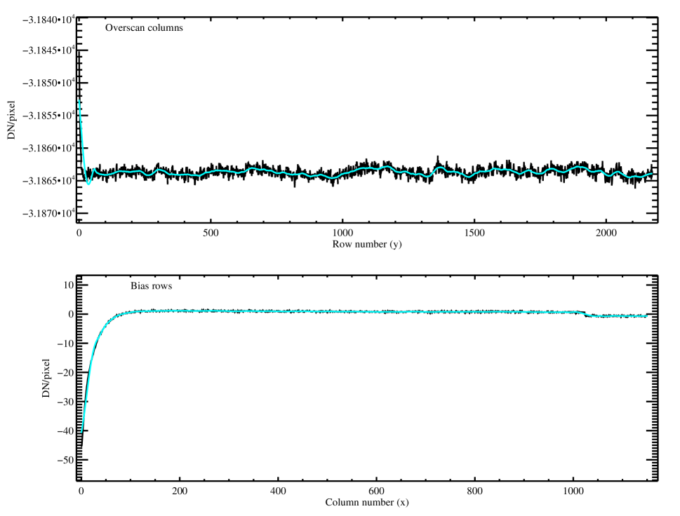
Refer to caption — Figure 1.— Upper panel: Sigma-clipped average of the overscan columns for a red-side frame (black data). Overplotted on this overscan average is the same data filtered by a SAVGOL function with 30 pixels (121 total native pixels) on each side. This method allows us to produce a smooth function that also recovers sharp features. Lower panel: Bias row from the same CCD. Overplotted is the data smoothed with a symmetric 37 pixel (73 native) SAVGOL filter.

We need to carefully model the overscan regions to remove the digital features in the CCD image. The first overscan region that is modeled includes all columns that readout immediately after each CCD row. First, we average these columns with 3-sigma clipping to produce a mean 1D overscan spectrum as a function of CCD row. Then the routine convolves this spectrum with a 4th degree Savitzky-Golay filter having a symmetric width of 121 native pixels average (Figure 1; upper panel). This averaged, filtered spectrum is replicated and subtracted from the entire, raw CCD frame. The same procedure is then applied to the set of rows immediately preceding the active CCD rows. Similarly, a 73 native pixel Savitzky-Golay filter is convolved with the average overscan in each column (Figure 1; lower panel). This result is replicated and subtracted from the entire CCD frame.

There have been two CCD detectors used with the blue side of the MIKE spectrometer. At commission, a SITe ST-002A CCD with relatively poor quantum efficiency (QE) at $\lambda<3800$ Å was installed. This CCD was replaced on May 6, 2004 with a Lincoln Labs CCID-20 device which has high QE down to the atmospheric cutoff. However, all data taken with the upgraded blue CCD between the dates of May 6, 2004 and September 21, 2005 suffer from a non-linearity in count rates. On the latter date, the voltages were reset to correct this non-linearity. To deal with this non-linearity in affected data, we adjust the raw CCD counts after overscan subtraction by multiplying this correction factor (CF) to the processed electron counts on a pixel by pixel basis:

	$\displaystyle{\rm CF(Image)}$	$\displaystyle=1,\;{\rm if\;Image}<14,000\;{\rm ADU}$
		$\displaystyle=2,\;{\rm if\;Image}>35,000\;{\rm ADU}$
		$\displaystyle=\exp{\left(\frac{{\rm Image}-14,000}{25,000}\right)^{2}},\;\;\;{\rm otherwise.}\;\;\;$

Any image pixel corrected to values over 50,000 electrons is capped artificially at that value, as this non-linearity correction is not reliable for such large corrections and one can assume these pixels are saturated.

After overscan subtraction, the image is trimmed to active CCD pixels and zero now represents the average level of the overscan regions. Assuming a flat-field of the pixel-to-pixel response has been created (see §5.1), the image is normalized directly by the pixel flat. The CCD gain is measured by assuming Gaussian statistics in pairs of flat-field images, and is applied (§5.1) so that all CCD images are converted from digital counts (ADUs) to electrons measured. We estimate the error on each pixel and report this as the inverse variance: $1/\sigma^{2}$ . The first estimate of this error is an approximation based solely on the measured number of electrons in each pixel as well as the global estimate of the readout noise in electrons. Gaussian statistics dictates that the variance is simply the number of counts in the expectation. For faint sources, the data provide only a very noisy estimate of the count rate. More importantly, one encounters a large systematic bias in the estimated error as the counts approach zero. In addition, the shape of the likelihood function starts diverging significantly from a simple Gaussian which is assumed in the rest of the pipeline. In order to ameliorate these effects we approximate the variance with this function:

\sigma^{2}=\left|{\rm Image(e^{-})}-\sqrt{2}\,RN\right|+RN^{2},

(2)

where Image(e^-) is the observed number of electrons and RN is the image readout noise measured in electrons. At very small Image(e^-) values, this approximation avoids having unreasonably small variance values. The final correction is simply an addition in quadrature with the variance added by using a pixel flat. This correction can be minimized by taking a long series of flat exposures.

The last step in the processing is to identify bad rows, passed in with the BADROWS keyword and subsequently set the inverse variance to 0. For MIKE, the first two and last two rows of each CCD seem to always carry excess counts and are flagged with zero inverse variance (zero weight) by default.

5. Flat-field Calibration

In this section, we describe the flat-field calibration frames and the algorithms which process and analyze these data. We use the frames for a variety of purposes, including (1) classic “pixel flats” for image correction of relative pixel-to-pixel CCD response, (2) “trace flats” for definition of the spatial echelle order boundaries, and (3) “slit flats” for the characterization of the spatial profile of a uniformly illuminated slit in each echelle order. We describe the implementation of each of these steps in detail below.

5.1. Pixel-to-Pixel flats

The first flat-field calibration routine, mike_mkmflat, produces a relative pixel flat-field image for both the blue and red cameras. The routine is straightforward: We use a stack of MIKE images obtained with the ‘milky diffuser’ in the beam directly behind the slit to obtain smooth flux distributions in both the spatial and spectral directions (these frames are referred to as milky flats). The practice of acquiring and analyzing a milky flat for pixel-to-pixel variations contrasts with standard practice in echelle spectroscopy. It has several advantages. First, we can correct for pixel sensitivity variations at and beyond the slit edge. This allows us to include several pixels at the slit edge boundary during sky subtraction and extraction. Second, stray light (including ghosts) which often exhibits sharp features at random angles with respect to the echelle orders is smoothed out and its effects are minimized. Third, it is easier to calibrate larger defects in the CCD and especially defects which partially cover an echelle order. Finally, one is assessing the pixel-to-pixel quantum efficiency with the same color light as the science exposures. Ideally, a stellar source is used in the blue milky flat to maximize counts at 3300Å and the internal flat-field lamp is used in the red to minimize the effects of sharp features (e.g. from atmospheric absorption features).

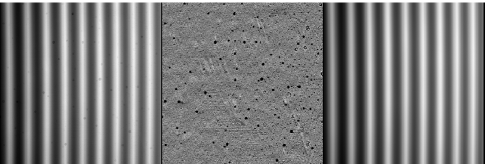
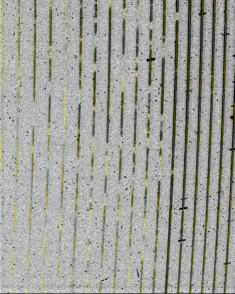
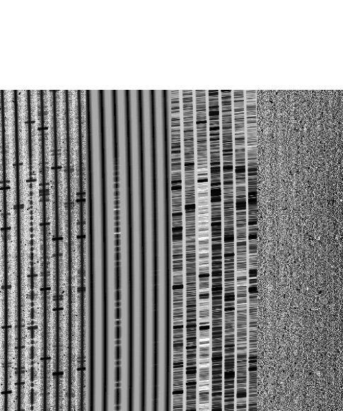
Each milky flat image is processed as described in $\S$ 4 and the stack of images is co-added to produce a single milky flat image for each CCD (a separate set of milky flats is required for each CCD binning used during data acquisition). We remove the large-scale flux variations as a function of position on the CCD (the routine default is to resample at the 256 native pixel scale). Then we apply a standard median filter in 1-dimension along CCD columns (in the spectral direction with a default width of 45 native pixels), on the assumption the calibration source has no small scale spectral features. This assumption breaks down for astrophysical sources with strong atmospheric telluric absorption bands observed with the red CCD. A 2-dimensional median filter (default median box is 9 native pixels on a side) is applied to the normalized milky-flat image processed above, and serves as a proxy for a model with which to reject the strongest features in the flat-field. Normalized milky-flat pixels are masked if they or a neighbor inside the median box size deviate by more than 3%. Finally, these masked pixels are replaced with a smoothed version of the normalized flat (with masked pixels given zero weight, and a 2-d smoothing length of twice the median box). The processed milky-flat is normalized by this final smooth image to effectively remove the remaining large-scale fluctuations and the resulting image is stored as the normalized pixel-to-pixel flat. In Figure 2, we show an example of the normalized flat-field of the red CCD in the middle panel. The co-added milky-flat image is shown before (left panel) and after (right panel) applying the processed pixel flat. One will notice that there are a large number of “pock” marks (moderate flat-field features) on the red Site CCD and the original blue Site CCD. They cover about 40 native pixels each and have an areal density of 5000 pixels per CCD. Reconstructing the pixel-to-pixel response as shown in Figure 2 is limited by a systematic error of approximately 1% per pixel. The statistical uncertainty in the pixel flat is saved, and applied to the statistical error (the inverse variance) on all images when the pixel flat is applied.

We calculate the gain between pairs of milky flats, with the estimator provided below. It is calculated from each pair of milky flats in sequence and the mean value is recorded for each image taken with this setup. A comparison image is made from the two flat images, $i1$ and $i2$ , as such:

	$\displaystyle image=$	$\displaystyle\sqrt{\frac{1}{\frac{1}{i1}+\frac{1}{i2}}}\,{\rm ln}[\frac{i1}{i2}\,\bar{\left(\frac{i2}{i1}\right)}]$			(3)
	$\displaystyle 1/<gain>=$	$\displaystyle variance(image).$			(4)

For a series of $N$ milky flat images, $N-1$ sequential pairings are analyzed, and the mean gain calculated from the $N-1$ pairings is used as the gain for all of the images being processed (with appropriate binning and side).

5.2. Trace Flats

A short set of direct flat images (without the diffuser behind the slit) is used to both define the echelle order boundaries and the relative spatial cross-section of the slit profile. The source can either be a short exposure of the internal flat-field lamp or the twilight sky. The internal lamp is better suited for defining the order boundaries, and the twilight sky provides a better direct illumination of the focal plane.

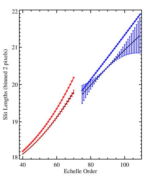
As with the Milky flats images above, a series of direct flat images are combined to yield a cleaned red and blue direct flat image, which we refer to as the combined “trace flats”. The peaks in each trace flat image are located after applying a sawtooth filter in the spatial direction (along rows). This procedure effectively locates the 50% level of both the left (positive peaks) and right (negative peaks) edges of the echelle orders in the trace flat images. Echelle orders in which 90% or more of the order was traced along the length of the CCD are considered good, and used to predict the edges of the remaining order. We then calculate the center and width of each echelle order, which are functions of CCD row number. The order width varies very slowly across the CCD array (see Figure 3), and can be described by a 2-dimensional polynomial which is linear with respect to row number and quadratic with respect to order number. We fit the order center with a Legendre polynomial as a function of CCD row number. We then use standard PCA analysis (Murtagh & Heck, 1987) of these order centers by searching for the principal components in the polynomial coefficients that describe the central column positions of the good orders. An example of these normalized basis functions are shown in Figure 4 in the left-hand panels (above and beyond the 0th order shape which is simply the mean order position on the CCD). The linear combination of the functions when multiplied by the smoothly varying coefficients shown in the main panel of Figure 4 accurately describe the order centers (for all rows and all orders) on the CCD. To predict the locations of the remaining orders which fall on the CCD, but which had poorly defined edges, we simply use the extrapolated coefficients based on the fits to the well defined order centers. Figure 5 shows an example of the order definition for a trace flat observed with the blue camera.

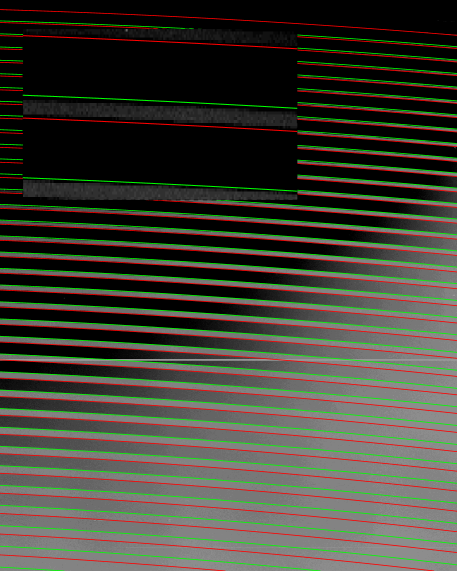
One might consider a slightly more simple procedure which is to extrapolate the polynomial coefficients describing the order centers as a function of order number. This usually produces unsatisfactory results due to the highly correlated condition of the coefficients. The principal components are defined to be orthogonal by definition, and the variation of each coefficients can be reliably extrapolated independently of the others. In the upper right corner of Figure 5, one notes order traces extrapolated into regions with nearly negligible flux. The decomposition of the left and right edges into order centers and order widths produced very reliable edge definitions, and allows for automated localization of the orders with no human interaction.

The pipeline routine responsible for determining the edge positions is called, mike_edgeflat, which produces an order structure with the prefix: OStr_ in the Flats directory.

5.3. Slit Profile Correction

The most involved correction derived from the flat-field calibrations is the slit profile correction, which we refer to as the “slit flat”. Once the echelle orders have been defined, and the wavelength image has been created from arc frame images (see $\S$ 6.3) we can measure the relative throughput of the spectrograph as a function of position along the 5^′′ slit length. Although simple in principle, we invoke a number of steps in order to reliably measure the slit profile. In the case of no correction, a spatially uniform source (like the dark night sky), would exhibit no change in the measured flux as a function of slit position. In order to correctly model the slit profile, the counts must approach zero in the gaps between the orders. A smooth scattered light image is constructed by fitting to the empirical counts in CCD pixels not associated with any echelle orders. The routine (x_modelslit) fits the scattered light row-by-row with 8 Legendre polynomial coefficients.

Each pixel in the trace flat is assigned three values in addition to the counts measured in the combined direct flat: order number, relative wavelength (recorded in pixels), and spatial slit position. The first two numbers are derived by the wavelength calibration procedures in the next section. The spatial slit position is measured as a quantity called slit fraction, which is normalized between -1 and +1, where -1 represents a pixel position exactly at the left edge of the slit-length, +1 is the right edge, and 0 is a pixel at the exact center of the slit. More precisely, these values are in units of half slit-length (HSL). A relative wavelength is given to each pixel by correcting for the tilt of the slit in the spectral direction and distance from the order center.

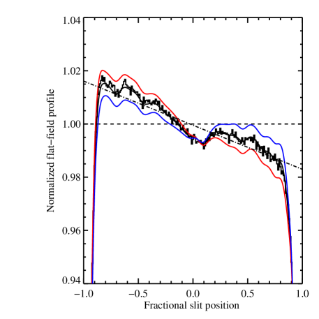
Order by order, the counts in each pixel are normalized by fitting a b-spline set of coefficients as a function of relative wavelength to the pixel counts in the central 70% of the slit ( $-0.7<HSL<+0.7$ ). The b-spline breakpoints are separated by 1.2 CCD pixels in the spectral direction, which is sparse enough to suppress the high-frequency noise but dense enough to fit real spectral features in the twilight sky. The smooth b-spline spectrum is evaluated at all pixels falling in the current order, and the counts in each pixel are normalized by this evaluated fit. In addition, the inverse variance in each pixel is scaled accordingly to preserve the reported signal-to-noise in each pixel (Figure 6).

Now the spatial profile in each echelle order is fit in two steps. The first step is to fit the mean profile, which is accomplished by fitting a single b-spline function to all of the normalized counts in the order as a function of slit fraction. The b-spline is evaluated at unit intervals of 0.01 HSL and stored from $-1.25$ to +1.25 HSL. The 251 samplings of the mean profile per order is stored in the structure with the tag PROFILE0. Any trend as a function of wavelength is fit with a linear dependence of row number and a b-spline fit to the residuals of the normalized trace flat about the mean evaluated b-spline. The typical linear deviations are around the 10% level along the length of a single order. These linear coefficients are sampled at the same 251 slit positions and stored as PROFILE1. One can reconstruct the appropriate slit profile for all rows in the order, for instance, the bottom row is given by PROFILE0 - PROFILE1 and the top row by PROFILE0 + PROFILE1.

The slit profile in each echelle order and the gradient of the profile with respect to position along the order are used to correct the spatial flux profile of the night sky before object extraction. The slit profile is not applied directly, given the low S/N region beyond the order boundaries, but rather the profile is used in the model basis of the sky background. We do find a difference in the recovered slit profile when a direct flat of the internal calibration lamp is compared to results of a direct flat of the twilight night sky. There is a significant linear gradient across the extent of the slit in the internal lamp images because of non-uniform illumination, and this slope is removed in the stored profile.

6. Wavelength Calibration

This section describes the series of algorithms that calibrate the wavelengths for every pixel that falls within the echelle footprint. Following standard practice, the wavelength calibration is derived from the spectrum of a ThAr lamp observed with the same setup as the science exposures. While the spectrograph in standard observing mode does not physically move, and so does not have flexure, the spectrum can move on the CCD by several native pixels over a night due to changes in the temperature of the air, glass, and metal in the spectrograph. Coeval calibrations are therefore important. Below, we will describe both the calibration of individual ThAr spectral images (“arcs”) and the strategy we employ for obtaining shifts in the echelle footprint over a night, and between science exposures and their “coeval” ThAr exposures.

Our approach to wavelength calibration differs from standard practice in that we generate a 2D wavelength image from each arc frame. To do so, we begin by deriving a 1D wavelength solution along the spatial center of each echelle order. We then trace the tilt of the ThAr lines out to the spatial edge of the order, and finally propagate the 2D solution for all pixels that fall within an order. It is worth noting that the tilt in the wavelength solution is advantageous to the data analysis in that it improves the sampling of sky lines, particularly near the Nyquist limit (i.e. narrow slit). Our specific treatment of this tilt is necessary because the tilt varies along and between echelle orders, and must be measured and accommodated across the full 2D spectrum to accurately subtract sky lines and extract the data.

6.1. Thorium-Argon Calibration Data

An internal Thorium-Argon (ThAr) hollow cathode lamp is used to obtain the required intensity and line density as a function of wavelength for calibration. When an arc image is taken, the switch that turns on the lamp also moves a small mirror into optical path between the telescope and the slit plate, blocking the light from the sky and allowing an F/11 image from the lamp (a bright spot, roughly 1 cm in diameter) to be projected onto the slit instead. This configuration is difficult to miss in the picture displayed by the slit-viewing camera and, as such, acts as a convenient safety feature for distracted observers who might otherwise take an arc simultaneously with a science exposure.

An exposure of 1-5 seconds provides sufficient lines for calibration of the full spectral range for all slit widths (0.35–2 arcsec). Our standard calibration template includes 12 lines in the bluest orders and 20–30 lines per order over most of the optical range. Strongly saturated lines dominate the appearance of the arcs around 7500Å. These do bleed electrons into neighboring columns, but they do not pose a calibration problem. A bigger issue is that the useful lines for calibration in the reddest orders ( $\lambda\gtrsim 7800$ , red order number less than 44) are fairly weak. Exposure times on the red side should be dictated by these weak lines if the reddest orders are of scientific interest.

In this pipeline, all wavelength calibrated data is converted from in-air wavelengths to vacuum wavelengths by default. It is important to realize that the change in the photon wavelength when traveling through a medium is a function of wavelength, unlike a Doppler shift, so that this conversion will affect any analysis, even if a Doppler shift is allowed.⁴⁴4The relationship between the wavelength of light in vacuum, $\lambda_{\rm vac}$ , and in a medium of index, $n$ , is $\lambda=\lambda_{\rm vac}/n(\lambda)$ . For air, $n-1=6.4328\times 10^{-5}+2.94981\times 10^{-2}/(146-\sigma^{2})+2.5540\times 10^{-4}/(41-\sigma^{2})$ , in which $\sigma=10^{4}/\lambda$ (Ciddor, 1996). This conversion can be avoided, as desired, but the reason for making vacuum wavelengths the default is that while optical–wavelength lines are typically discussed at “in-air” wavelengths, UV–wavelength lines are always discussed at “in–vacuum” wavelengths. Consequently the standard for galaxy and stellar spectroscopy is in–air wavelengths, while the standard for QSO absorption line observations is in-vacuum. To understand the implications of this conversion, it is important to think about how the lines are produced and how the data are recorded. First, the photons from both astronomical sources and calibration lamps are produced in a vacuum, travel in air through the spectrograph, and are detected in a dewar under vacuum⁵⁵5As a pedagogical point, we note that the only record of the wavelength of a photon in a spectrograph is its location on the CCD, which is determined by the angle of the photons after reflection from the grating. Thus, any spectral features from any source will be recorded at in–air wavelengths.. The wavelengths designated to the lines in the arc spectrum will determine the definition of the wavelength calibration, and it will be appropriate for both astronomical sources and calibration lamps. If the line list for the arc lines gives in–air values, then the calibration is in-air and must be converted to vacuum to discuss UV wavelength lines.

6.2. Standard Calibration

The first algorithm follows standard practice for echelle reduction. We perform basic overscan and bias subtraction and then flatten the blue CCD as described in the previous sections. With the red CCD, however, we skip the overscan subtraction (although the average value is written to the bias row) because the very bright arc lines near above 7500Å tend to bleed into the overscan region. The code then calculates the image shift between the arc frame and the trace flat solution as described below.

For every echelle order, the code performs a pseudo-boxcar extraction by rectifying the order with linear interpolation and extracting the central column of each order. The individual order extractions are stitched together to create a single array. This array is cross-correlated against the same construction from an archived, calibrated image using an FFT algorithm. The peak in the FFT sets the shift between the stitched 1D arcs of the archived and new arc images. The derived shift is then used to identify the physical order numbers of the new arc and to also predict the average shift in the spectral direction (e.g. due to changes in the echelle angle).

Each echelle order is then analyzed individually. Its 1D spectrum is cross-correlated with an FFT to the single-order 1D archived spectrum to improve the precision of the spectral shift. The code then derives a wavelength solution for the new 1D spectrum assuming the archived solution with the derived offset. The algorithm then identifies all ThAr arc lines using a peak finder which demands a high signal to noise ratio (SNR) and a ‘pointed’ feature whose fluxes in the central five pixels $f_{i}$ are appropriately rank ordered ( $f_{1}<f_{2}<f_{3}>f_{4}>f_{5}$ ). Those lines that satisfy this rank ordering and lie within three binned pixels of a laboratory-calibrated ThAr line are centroided and recorded. The line centroid is measured by (i) splining the flux of the central seven pixels, (ii) evaluating the peak of the spline, (iii) identifying the left-hand and right-hand edges of the spline corresponding to 33% of the peak, and (iv) averaging the two edges to derive the centroid. This algorithm is non-parametric and robust. The result is a high SNR subset of ThAr lines with measured pixel centroids and known laboratory wavelengths.

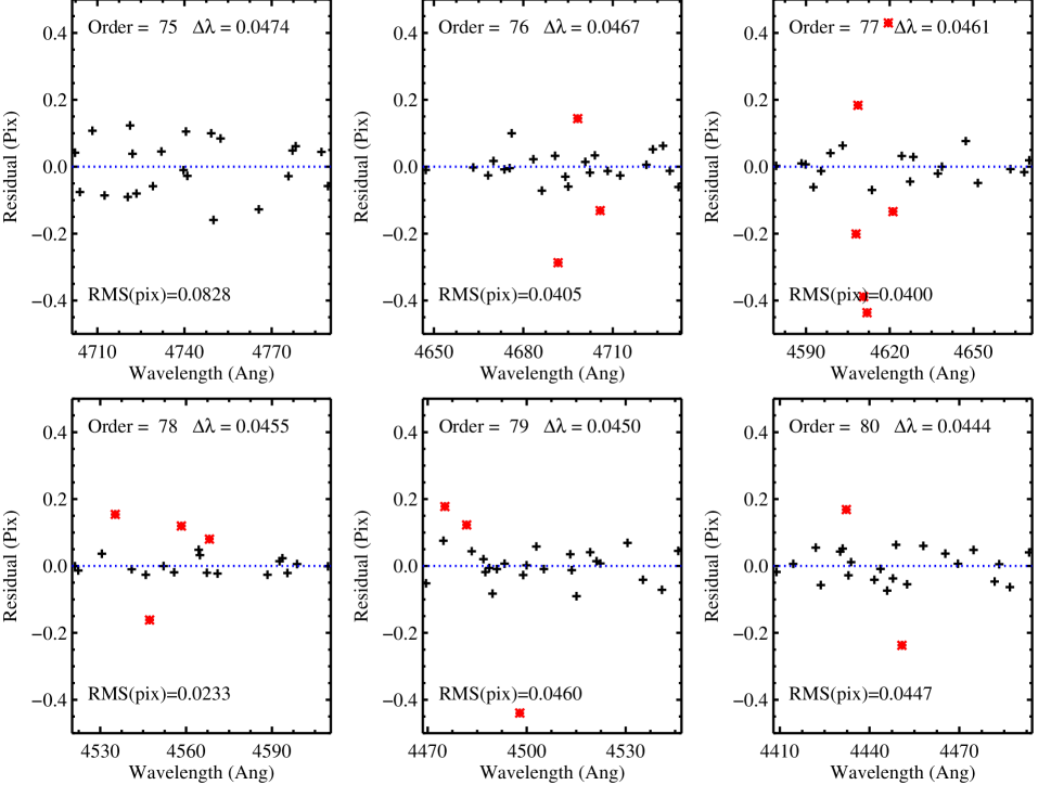
The code then performs a low order, Legendre polynomial fit with aggressive rejection to the pixel values versus the logarithm of the laboratory wavelengths. By imposing the logarithm of the wavelength, one significantly reduces a systematic bias which favors long–wavelength lines. This is less important for individual echelle orders (where the wavelength range is only $\approx 100$ Å), but it is critical for the 2D polynomial fit described below. Finally, the code again searches for ThAr lines in the 1D spectrum but using this fit for the wavelength solution and also allowing lines with lower SNR in the image. A final 4th or 5th order Legendre polynomial fit is derived, again with aggressive clipping. The final output for each order includes the 1D spectrum and the pixel centroids and ThAr wavelengths of all the ‘good’ ThAr lines that were not rejected during the Legendre polynomial fits. Figure 7 presents the residuals for Legendre fits to echelle orders 75 to 80 from the blue camera of MIKE. In nearly every individual order, we achieved line residuals of RMS $<0.1$ pix and a fit solution with RMS $<0.05$ pix independent of binning.

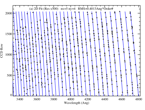
The next algorithm performs a 2D fit to all of the good⁶⁶6Future updates to the code will include a trimmed ThAr linelist constructed using the algorithms described in Murphy et al. (2007). ThAr lines for all of the echelle orders⁷⁷7Note that orders run (mostly) parallel to columns and with row numbers changing along the order.. The algorithm inputs the pixel (row number of the line centroid), wavelength, and echelle order for each fitted line. It then performs a 2D Legendre polynomial fit $P_{jk}(m,y)$ to the product of the arcline wavelength $\lambda_{i}$ and its echelle order $m_{i}$ as a function of (i) the echelle order number and (ii) the row number $y_{i}$ (e.g. http://iraf.noao.edu/)

m\lambda=P_{jk}(m,y)\;\;\;\;.

(5)

With this basis, a well-behaved fit can be derived with 20 parameters (four spectral and five along the prism dispersion [ $j=5,k=4$ ]); the typical RMS is $\approx 0.2$ (Å order#). By performing a 2D solution, one more confidently interpolates (and occasionally extrapolates) over regions of the arc image where there is a low density of calibrated ThAr lines. This is particularly important at the reddest wavelengths where there are many fewer lines for analysis.

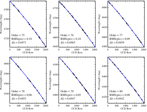
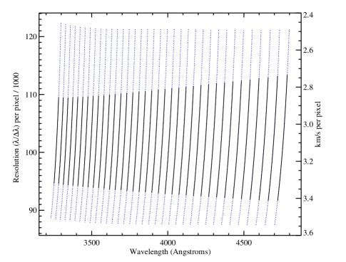
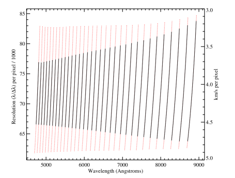
The resulting 2D fit describes the wavelengths along the center of each echelle order on the CCD. Figure 8a shows the full 2D solution for one example image as a function of row number. Figure 8b shows the solution for a subset of echelle orders and the measured RMS of the fit. Again, we generally achieve residuals of RMS $<0.1$ pix (binned) in each echelle order for the 20 parameter Legendre polynomial. Using the 2D solution, we can calculate the dispersion as a function of wavelength over the entire footprint of spectrum. In Figure 9, we present the wavelength dispersion of the spectrometer as measured for an unbinned spectrum (native pixels of 15 $\mu$ m).

6.3. Wavelength Image

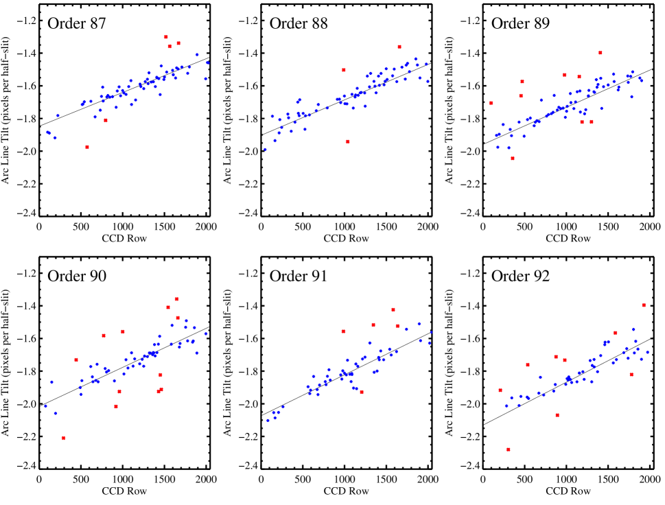
The algorithms discussed in the previous section generate a 2D Legendre polynomial fit describing the wavelength value down the center of each echelle order. We now describe the algorithms which extend the wavelength solution throughout the full echelle footprint. The algorithms first identify and trace all high S/N arc lines in each order across the chip. In this manner, we measure the tilt of the lines as a function of wavelength and echelle order. Specifically, we identify all 5 sigma peaks in the spectrum, independent of whether the peak corresponds to a well-calibrated ThAr line. We then trace the centroid of each line from the center of the order to the order edges using the IDLSPEC2D algorithm trace_crude. We found that each arc line is well described by a straight line (i.e. a slope); the code measures and records the best-fit slope for each arc line. Figure 10 presents the measured slopes for the ThAr lines as a function of CCD row in several echelle orders (blue camera). In general, one has over 30 lines per echelle order for analysis. It is evident that the arc-line slopes vary across each echelle order. This is because the quasi–littrow angle ( $\gamma$ ) changes as a function of position in the focal plane.

Similar to the analysis of the ThAr wavelengths, we fit a 2D Legendre polynomial to the slopes of the arc lines across the full CCD. This 2D solution enables one to interpolate through regions of the CCD with a lower density of ThAr lines. Together the wavelength values and arc line tilts at the center of each order is sufficient for assigning a unique wavelength to the center of every pixel on the CCD that falls in an echelle order footprint. This is done for all applicable pixels and a wavelength image is written to the disk for each arc frame. We do not solve for the case when orders overlap and assume a unique wavelength value for each pixel in the image. This wavelength image is calibrated in air and is stored with logarithmic values. By default, the pipeline associates each scientific exposure with the wavelength image whose arc frame has the smallest difference in UT time from the start of each exposure. We do not interpolate between arc frame exposures, and simply use the nearest exposure in time.

6.4. Image Shift

As described in $\S$ 2, the footprint of the MIKE spectrometer is observed to shift throughout the course of the night, presumably because of thermal changes. Therefore, the footprint which is traced by the flats acquired in the afternoon ( $\S$ 5.2) is generally offset from the one observed during the night. We measure this shift from the inner 17 orders using an algorithm similar to the one which measures the slit profile ( $\S$ 5.3). In this case, however, the algorithm is applied to the arc images. As with the slit profile, one must first have a good estimate of the slit tilt throughout the image. Therefore, the steps described in the prior two subsections are first applied to one arc image (the slit tilt does not vary significantly as the image shifts).

In each order, the code collapses all pixels with signal greater than 10 electrons as a function of distance from the center of the slit, normalized to $\pm 1$ by the average order width.

We then measure the center of the arc profile by identifying where the flux dips to $40\%$ of the peak on each side of the profile and average the two edges. This center is compared with zero and gives the shift in pixels of the image parallel to the rows (the shift along the columns is negligible). This process is performed on the 17 central orders and the best linear fit to the shift as a function of order number is found. The parameters of this fit are recorded in the main structure (in the ARC_XYOFF tag) and are used to shift the archived footprint onto the science and arc images.

7. Object Tracing and Extraction

7.1. Tracing

The final phase in the reduction of two-dimensional CCD images to 1-dimensional spectra involves the final localization and extraction of a single object in each MIKE exposure. The first step involves the tracing of the object, the definition of the object position with respect to the spatial position of the echelle orders. A first estimate of the local sky background is calculated by masking pixels within the object aperture (default is the central 3.75^′′ of the 5^′′ slit) and those with a slit profile value below 30%. The remaining steps incorporate an iterative series of object profile reconstruction as a function of wavelength and echelle order, slight tweaking of the initial object position given the mean object profile in each order, and finally, combined object and background extraction.

Once the echelle orders have been defined by the trace flat images, we determine the best spatial shifts from the traceflats to the appropriate arcframe associated with each science image (see §6.4). Each echelle order in the science frame is rectified (just for the object tracing) with the shifted order boundaries. The rectified order is collapsed along columns with median smoothing to reject unflagged cosmic rays and bad pixels. In the collapsed vector of each order, we locate the most significant peak within the slit and associate the fractional position between the order boundaries as the first guess for the location of the object where 0.5 corresponds to the center of the slit-length. If the object is detected in seven or more echelle orders, the fractional positions in the undetected orders are predicted by a simple linear fit to the detected positions as a function of order number. The fractional positions for the rectified orders (whether measured or predicted) are converted back to CCD pixel coordinates on the original science image based on the shifted order boundaries. We measure the object peaks in each CCD row in each order by iteratively calculating a flux-weighted mean of the object counts. The peak measurement is unbiased for well sampled profiles, but is subject to CCD artifacts and sharp sky features. Each set of object centers, called a trace, is fit with a 6th order Legendre polynomial weighted by estimated errors in the flux weighted centroids (with an additional floor of 0.01 pixel error added in quadrature). In the fitting procedure, centroids which deviate by greater than 10 $\sigma$ from the polynomial fit are masked.

Echelle orders in which less than 50% of the measured centroids are rejected are considered useful for a subsequent PCA analysis (similar to the order-tracing analysis described in §5.2). The polynomial coefficients from 1st to 6th order of the well constrained echelle orders are combined into orthogonal eigenfunctions. The useful traces are checked to see if their eigenvalues (PCA coefficients) agree with simple interpolated predictions of the other traces. The worst outliers with a 1 pixel deviation in the primary eigenvalue or a 0.3 pixel deviation in the secondary eigenvalue level are rejected. The remaining eigenvalues are fit as a function of echelle order with low-order polynomials to predict the previously rejected traces, with a quadratic fit to the leading eigenvalues and a linear fit to the secondary eigenvalues. The remaining coefficients are simply replaced with the median value of all the good values.

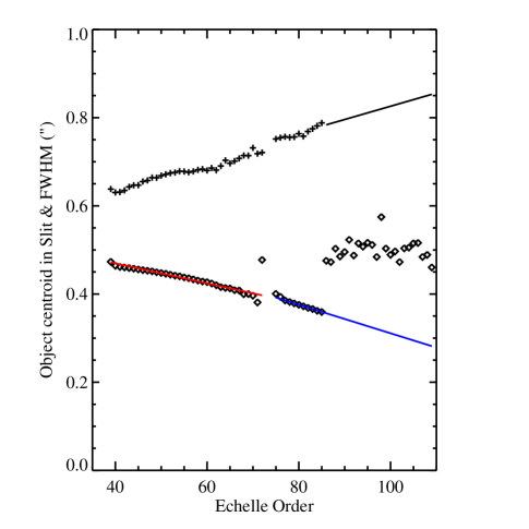
We calculate the mean trace position (the average spatial position of each trace over all rows) with the following steps. First, we remove the high-order variations (tilt, curvature, etc.) by summing up the contributions from 1st order to 6th order and subtracting the sum from the measured mean trace position. Second, the best quadratic fit to the mean residual trace positions are found, and the higher order contributions (orders 1–6) are added back. The result is a trace of the object in each echelle order that relies on the principal components of the well traced orders and smooth fits to these coefficients. Finally, we perform a last iteration and allow the traces which have sufficient signal-to-noise to adopt the empirically determined trace centers. Object traces with low signal-to-noise or partial orders retain the interpolated values derived above. We show how the object trace can move relative to the center of the echelle order positions as the bottom set of open diamonds in Figure 11. The routine invoked for object tracing is called mike_fntobj. An example of the final determined positions for an object observed with MIKE is shown in Figure 12.

7.2. Object Profile Definition

The next step in object extraction is to estimate the sky background as a function of wavelength and echelle order number. Because this estimate is only used to derive the spatial profile of the object PSF, accurate fitting of narrow emission lines is not critical. Some fraction of the background arises in diffuse scattered light, and this is estimated by interpolating the pixel counts in the gaps of the echelle orders to all of the CCD. Once the scattered light estimate has been subtracted, the remaining sky background is fit in each echelle order. A subset of the pixels in each order are used if they fall at least 1.9^′′ from the object centroid and have a slit profile value greater than 30%. For standard stars, the default is to only use pixels at least 2.25^′′ from the object, although one is recommended to skip sky subtraction for very bright targets. The pixels designated from sky estimation are corrected by their corresponding slit profile values. These corrected pixels are then fit with a b-spline as a function of wavelength using the wavelength image map calculated in §6.3. The breakpoints defining the b-spline function are spaced with a separation of 1.2 times the local wavelength dispersion per pixel. After the b-spline fit has converged, sky subtraction is as simple as evaluating the b-spline function for all pixels in the echelle order, correcting by the slit profile (multiplying) and subtracting the product from the scattered-light subtracted image. The routine that performs the initial sky-subtraction on all science images is called mike_skysub.

At this stage of the reduction, we finally have a fully characterized science image (i.e. flat-fielded, traced, wavelength calibrated, and background subtracted), and can perform optimal extraction in the empirical sense (e.g. Horne, 1986) once the object profile is characterized as a function of wavelength. With higher signal-to-noise spectra, we can determine subtle variations in the object profile. Below is the set of steps we follow to characterize the object profile which is then used to optimally extract the 1-dimensional spectrum in each echelle order. The list below is repeated iteratively for a default of three times, but can be set by the user when invoking the extraction algorithm mike_box.

The first step is a standard boxcar extraction in each order, using an aperture with a default spatial extent of 3.5^′′ centered on the object trace. The boxcar extraction, along with the associated variance array, is stored in the final object extraction structure. The median signal-to-noise ratio (MSNR) is calculated for the boxcar spectrum in each echelle order, and after this point, the orders are processed in order of decreasing MSNR.

The boxcar extraction is median smoothed and compared to the original spectrum to identify cosmic rays and other deviant spectral pixels. The non-deviant pixels are fit with a b-spline function with a breakpoint spacing that is twice the local pixel dispersion (i.e. every 2 spectral pixels). In this step, we are fitting for the spatial profile, so we normalize each CCD pixel in the 2D image by the boxcar extracted counts at the appropriate wavelength (the bspline function representing the boxcar extracted flux is evaluated at every pixel in the order footprint). The pixels in the resulting normalized image have, by definition, a total spatial cross-section of unity in the boxcar region. This definition is one method to tie the optimally extracted fluxes to the same system as the boxcar extracted values.

The object profile is fit with one of three methods based solely on the MSNR determined for that echelle order. If the MSNR is less than 2.5, then a uniform Gaussian profile is adopted with a fixed width. If at least 2 higher MSNR orders have been extracted (earlier in the processing), then the width of the Gaussian profile is extrapolated from the processed orders. If an estimation of a width based on other profiles is not available, then a fixed width of 0.7^′′ is assumed (comparable to the median seeing at Las Campanas). If the MSNR is greater than 2.5, then a Gaussian is not assumed, and a full spatial profile is fit. If the square of MSNR is greater than 500, then the spatial profile is allowed to vary as a quadratic function of wavelength along the order. Otherwise, a uniform profile is fit to all pixels in the order. Even in the high MSNR case, a uniform profile is fit to the order, but the full variable profile is used in object extraction. The full-width, half-maximum (FWHM) is calculated empirically from the uniform profile and is used as a prior for subsequent lower MSNR orders. In Figure 11, the calculated and extrapolated estimates of the spatial FWHM are shown as a function of echelle order.

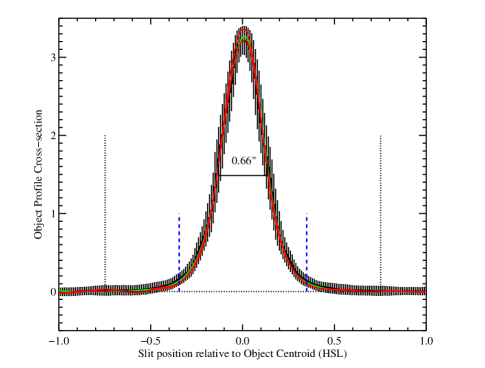
The biggest difficulty with an empirical determination of the object profile are the wings of the profile. These need to be well behaved to perform accurate extractions. In this implementation, we specify a separation from the object centroid, past which we extrapolate an exponentially decaying wing. The separation increases as a function of MSNR, such that higher MSNR orders require less extrapolation. To extrapolate, we find the best linear fit to the logarithmic profile as a function of spatial distance from the object centroid. We perform the extrapolations on left and right sides of the profiles separately and in each case we fit to the shape of the profile from the half-maximum to the cutoff distance determined by the MSNR above. This procedure is very robust in practice and delivers realistic wings for the object profiles. The slope of the extrapolation is forced to be less than $-1.0$ , because a higher slope would not have finite flux if extended to infinity. In Figure 13, we show an example of the object profile determined in a single MIKE echelle order. The ticks denote the extent of the scatter in the normalized image counts, while the solid lines represent the spatial object profile fit as described by a b-spline.

7.3. Extraction

Just before the actual extraction occurs, we perform a check and correction to the object tracing. Now that we have a well determined empirical profile for the order, we test the correlation of the profile at the current position compared to shifting the profile one pixel left or right. This check is done at each row in the echelle order, and we apply a smooth fit of the deviation away from zero offset. The trace correction is added to the object centroid array and is applied in the next iteration.

Extraction is performed by fitting in the least squares sense to the full echelle order footprint with a simple linear model:

Model(x,\lambda)=OS(\lambda)*OP(x,\lambda)+SS(\lambda)*SP(x,\lambda),

(6)

where x is in units of HSL, and $\lambda$ is wavelengths. OS and SS are the object spectrum and sky spectrum, respectively, while OP and SP are the previously determined object profile and slit profile, respectively. The extraction is a simultaneous b-spline fit of both the object spectrum and the sky spectrum. The breakpoints for each spline are separated by exactly the local wavelength dispersion. For a standard MIKE echelle order which is 2048 rows high (spectral binning of 2), there will be approximately 4096 free parameters in the simultaneous b-spline fitting. We then search for pixels deviating by greater than 10-sigma, and mask those pixels as well as the 12 closest neighbors under the assumption that these are cosmic rays. During the final iteration, one last b-spline fit is performed with the final masking, and both the object and sky splines are sampled with uniform velocity dispersion on a fixed wavelength grid to facilitate combining multiple science exposures (Figure 14). One can output the model fits of the two-dimensional sky image, object image and object profile.

8. Endgame

In this section, we discuss the procedures which combine and flux calibrate the extracted spectra (in separate echelle orders). The end product is a continuous, 1D spectrum calibrated to energy units with a relative accuracy of better than $10\%$ over 100Å spectral regions. In practice, this involves combining the multiple exposures of a single target, fluxing, and then coadding the individual echelle orders. We present separate discussions of fluxing and coaddition.

8.1. Fluxing

Spectra acquired with echelle spectrometers are notoriously difficult to calibrate in absolute flux units. This can be attributed to a number of factors: narrow slits, scattered light, vignetting. It is generally difficult to achieve even an accurate relative fluxing of the data (e.g. Kirkman et al., 2003; Ellison et al., 1999; Suzuki et al., 2003). Furthermore, little attention is given to this problem because the analysis of echelle data usually involves normalizing the object’s continuum flux level prior to measuring the optical depth and/or equivalent width of spectral features. In this respect, fluxing is mainly a convenience but not a necessity. Nevertheless, the MIKE instrument has several characteristics which make it better suited to accurately flux (see the Introduction).

We implement algorithms which follow standard procedure to generate a sensitivity function from observations of a spectrophotometric standard. This sensitivity function converts measured electrons per second per Å to flux units (erg s^-1 Å^-1 $\,{\rm cm^{-2}}$ ). It is determined by comparing the electron flux of the spectrometric standard with its absolute, previously calibrated flux. No corrections are made for slit losses or atmospheric extinction. These efforts are relatively shallow functions of wavelength and should not substantially affect the relative flux on scales smaller than 100Å. Furthermore, if one observes the science objects and standard under similar seeing conditions and at similar airmass, then these losses will be partially corrected.

The only significant challenge that we faced is that no spectrophotometric standards have been observed at echelle resolution. As such, we found it impossible to derive an accurate sensitivity function in spectral regions corresponding to absorption features in the standard star (e.g. the Balmer series). In low dispersion spectrometers, one can clip these features by fitting a low order polynomial to the sensitivity function. In echelle data, however, a strong Balmer line can encompass one or more echelle orders. For this reason, one should observe calibration standards with weak absorption lines. We also designed a graphical user interface which enables the user to identify and mask out absorption features when generating the sensitivity function. This is generally successful, although systematic errors are significant when the features coincide with the peak or edge of an echelle order.

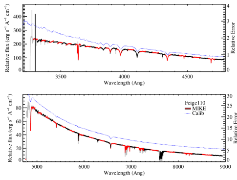
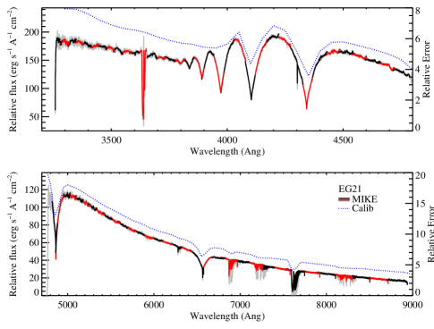
In Figures 15 and 16 we present the fluxed spectra of two standard stars observed on 02 September 2004 with a 1^′′ slit under photometric skies. We calibrated these stars (as described above) by generating a sensitivity function from the spectrophotometric standard NGC 7293 observed at 1.11 airmasses. The spectrum of EG21 (Figure 15) represents a nearly optimal example. The flux in overlapping regions of echelle orders is well matched, the strong Balmer lines have appropriate shape, and the relative flux matches the calibrated values (Hamuy et al., 1994) to better than 5 $\%$ for $\lambda>3800$ Å. At bluer wavelengths, the flux is underestimated because of additional slit losses and atmospheric extinction; the star was observed at a higher 1.36 airmasses. The results for Feige 110 (Figure 16) are more representative. There is a modest mismatch in the flux of overlapping echelle orders, especially the first $\approx 10$ orders in each camera. The mismatch is less than 10 $\%$ , however, and the combined spectrum (grey) follows the ‘true’ calibration. The relative fluxing is better than 10 $\%$ redward of 4000Å, and the spectrum underestimates the flux at bluer wavelengths for the same reasons as EG 21. We emphasize, however, that the relative flux is excellent over spectral regions of less than 100Å.

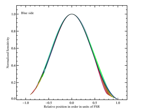
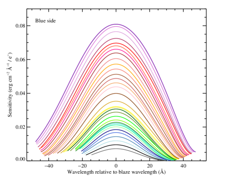
It is instructive to analyze the sensitivity function to investigate the blaze function and instrumental response of MIKE. Figure 17 describes the blaze function, normalized to unit flux at peak, for the blue camera as derived from the sensitivity function. The blaze function profile is nearly constant with echelle order when plotted as a function of the free spectral range (FSR). The shape is well modeled by a 9th order Legendre polynomial. which is the default function form for fitting the sensitivity function, which is shown in Figure 18.

8.2. Coaddition

There are two important aspects to producing a final 1D spectrum from a series of science exposures: the coaddition of multiple exposures and the combination of overlapping echelle orders. The specific ordering of our algorithms are: (1) coadd multiple exposures of each echelle order; (2) flux the individual echelle orders; and (3) combine the echelle orders to produce a final, continuous 1D spectrum. We prefer this ordering because it maximizes the signal-to-noise for combining echelle orders, whose blaze edges may have relatively low signal. Furthermore, the instrument is sufficiently stable that one can successfully combine individual echelle orders from multiple nights in an observing run without fluxing first. The fluxing algorithms were discussed above; we now detail the coadding procedures. We remind the reader that the spectra have been extracted onto a fixed wavelength grid. No rebinning is required and registration of the spectra is trivial.

The combination of multiple science exposures of the same object is performed separately on each echelle order, in sequence of red to blue. The orders are averaged together, weighting by the square of the median S/N ratio after first flagging outliers (generally due to low-level cosmic rays). To carry out this calculation, one requires two quantities: (i) the median S/N ratio for weighting the data; and (ii) a scale factor which normalizes the spectra to a common intensity. The latter is necessary for properly averaging data when clipping outliers. These quantities are calculated relative to a designated ‘template’ exposure, preferably the frame with largest signal.

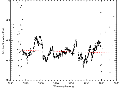
All pixels with S/N $>2$ (designated HSNPIX here) are identified in the template exposure. If there are over 100 HSNPIX, then the median S/N is measured from these pixels. Otherwise, the code adopts weighting factors based on the relative exposure times. The algorithm also calculates a scaling factor by comparing the fluxes of the HSNPIX for each exposure relative to the template. Figure 19 presents an example of the relative flux for echelle order 91 of the blue camera for a pair of 2400s exposures taken in sequence. We show only the HSNPIX and have median smoothed by 100 pixels. The median S/N per pixel is 6 for the template exposure. The algorithm scales the data differently depending on the number of HSNPIX. If there are over 300 HSNPIX, a line is fitted to the relative fluxes (median smoothed by 100 pixels) as a function of wavelength and applied to the full spectrum (Figure 19). If there are 100 to 299 HSNPIX, then the scale factor is the median of the relative fluxes. For fewer than 100 HSNPIX, we adopt the relative exposure times as the scale factors.

The median S/N and median scale factors are recorded for each echelle order, in turn. After all of the echelle orders are analyzed, the algorithm re-evaluates the two quantities for those orders with fewer than 100 HSNPIX. The code takes the median values of the two quantities from the nearest 5 orders that have (i) greater than 100 HSNPIX and (ii) lie within 10 orders, if these conditions are met. This is implemented primarily on orders where a very large absorption feature (e.g. a damped Ly $\alpha$ line) has significantly depressed the S/N of a single echelle order.

After scaling the data, the algorithm compares the scatter between multiple echelle orders with the scatter predicted from the variance array. As described in $\S$ 4, the variance array includes estimates of the uncertainties associated with counting statistics and read noise. In general, we find that the scatter predicted from the variance array is 10 to 20 $\%$ lower than the observed scatter in multiple exposures. This could be explained by a modest overestimate of the CCD gain, but the algorithms which derive the gain are proper. We suspect that the additional scatter is due to systematic errors introduced by flat-fielding, sky subtraction, and wavelength calibration. Our solution is to scale the variance arrays of all the exposures of a given echelle order by a single factor. In this manner, we demand that the observed scatter is consistent with that predicted from the variance arrays assuming $\chi^{2}$ statistics.

If there are three or more exposures then the code flags and excludes any pixels that deviate by more than 5 $\sigma$ from the median value. Clipping is rare for optimally extracted data (or short exposures of bright targets) and it is not necessary to repeat this step. Finally, the data are averaged with weights proportional to the median S/N squared. The resulting data product is a series of combined, individual echelle orders. These data are fluxed with the sensitivity function derived from a spectrophotometric standard, as described in the previous section.

The final step is to combine the edges of overlapping echelle orders. Again, no rebinning is necessary and registration is trivial because the data were extracted onto a fixed wavelength grid. In the previous sub-section, we noted that the relative flux of the overlapping spectral regions generally agree to within 10 $\%$ (Figures 15,16). Therefore, we simply average the data, weighting by the variance of each pixel. Aside from a small spectral region, one of the echelle orders will dominate the signal in the overlap region.

9. Summary

We have described the software package MIKERedux designed and developed to reduce the echelle images produced by the MIKE spectrometer. This code is publicly available and its primary algorithms have been applied to data reduction for other modern spectrometers. While development of this package has halted, one of us (JXP) plans to release a Python-based code following many of the procedures described here.

The strategies and implementations discussed here are the result of many fruitful conversations with our colleagues. In particular, JXP acknowledges Dan Kelson for inspiring some of the algorithms described here during the time they overlapped at Carnegie, and RAB thanks Steve Shectman for the countless days spent discussing all aspects of (and building) MIKE. We further thank R. Cooke for his comments and criticisms on a draft of the manuscript.

References

Bernstein et al. (2003) Bernstein, R. et al. 2003, in Instrument Design and Performance for Optical/Infrared Ground-based Telescopes. Edited by Iye, Masanori; Moorwood, Alan F. M. Proceedings of the SPIE, Volume 4841, pp. 1694-1704 (2003)., 1694.
Chen et al. (2005) Chen, H.-W. et al. 2005, ApJ, 634, L25.
Churchill & Allen (1995) Churchill, C. W. and Allen, S. L. 1995, PASP, 107, 193.
Ciddor (1996) Ciddor, P. E. 1996, Appl. Opt., 35, 1566.
Dekker et al. (2000) Dekker, H. et al. 2000, in Proc. SPIE Vol. 4008, p. 534-545, Optical and IR Telescope Instrumentation and Detectors, Masanori Iye; Alan F. Moorwood; Eds., ed. M. Iye and A. F. Moorwood, 534.
D’Odorico et al. (2006) D’Odorico, S. et al. 2006, in Ground-based and Airborne Instrumentation for Astronomy. Edited by McLean, Ian S.; Iye, Masanori. Proceedings of the SPIE, Volume 6269, pp. 626933 (2006).
Dupree et al. (2007) Dupree, A. K. et al. 2007, ArXiv Astrophysics e-prints.
Ellison et al. (1999) Ellison, S. L. et al. 1999, PASP, 111, 946.
Ellison, Prochaska & Lopez (2007) Ellison, S. L., Prochaska, J. X., and Lopez, S. 2007, MNRAS, 380, 1245.
Faucher-Giguère et al. (2008) Faucher-Giguère, C.-A. et al. 2008, ApJ, 681, 831.
Hamuy et al. (1994) Hamuy, M. et al. 1994, PASP, 106, 566.
Horne (1986) Horne, K. 1986, PASP, 98, 609.
Kelson (2003) Kelson, D. D. 2003, PASP, 115, 688.
Kirkman et al. (2003) Kirkman, D. et al. 2003, ApJS, 149, 1.
Meiring et al. (2007) Meiring, J. D. et al. 2007, ArXiv Astrophysics e-prints.
Murphy et al. (2007) Murphy, M. T. et al. 2007, ArXiv Astrophysics e-prints.
Murtagh & Heck (1987) Murtagh, F. and Heck, A. 1987, Multivariate Data Analysis, (Dodrecht: Kluwer).
Prochter et al. (2010) Prochter, G. E. et al. 2010, ApJ, 708, 1221.
Suzuki et al. (2003) Suzuki, N. et al. 2003, PASP, 115, 1050.
Vogt et al. (1994) Vogt, S. S. et al. 1994, in Proc. SPIE Instrumentation in Astronomy VIII, David L. Crawford; Eric R. Craine; Eds., Volume 2198, p. 362, 362.