The Keck $+$ Magellan Survey for Lyman Limit Absorption III: Sample Definition and Column Density Measurements

Abstract

We present an absorption-line survey of optically thick gas clouds – Lyman Limit Systems (LLSs) – observed at high dispersion with spectrometers on the Keck and Magellan telescopes. We measure column densities of neutral hydrogen $N_{\rm HI}$ and associated metal-line transitions for 157 LLSs at $z_{\rm LLS}=1.76-4.39$ restricted to $10^{17.3}\,{\rm cm^{-2}}\leq N_{\rm HI}<10^{20.3}\,{\rm cm^{-2}}$. An empirical analysis of ionic ratios indicates an increasing ionization state of the gas with decreasing $N_{\rm HI}$ and that the majority of LLSs are highly ionized, confirming previous expectations. The Si⁺/H⁰ ratio spans nearly four orders-of-magnitude, implying a large dispersion in the gas metallicity. Fewer than 5% of these LLSs have no positive detection of a metal transition; by $z\sim 3$, nearly all gas that is dense enough to exhibit a very high Lyman limit opacity has previously been polluted by heavy elements. We add new measurements to the small subset of LLS ($\approx 5-10\%$) that may have super-solar abundances. High Si⁺/Fe⁺ ratios suggest an $\alpha$-enhanced medium whereas the Si⁺/C⁺ ratios do not exhibit the super-solar enhancement inferred previously for the Ly$\alpha$ forest.

1. Introduction

As a packet of ionizing radiation ($h\nu\geq 1$ Ryd) traverses the universe, it has a high probability of encountering a slab of optically thick, H I gas. For sources in the $z\sim 4$ universe the mean free path is only $\approx 30$ Mpc (physical; Worseck et al., 2014), i.e. less than 2% of the event horizon. Observationally, researchers refer to this optically thick gas as Lyman limit systems (LLSs) owing to their unmistakable signature of continuum opacity at the Lyman limit ($\approx 912$Å) in the system restframe. A fraction of this gas lies within the dense, neutral interstellar medium (ISM) of galaxies, yet the majority of opacity must arise from gas outside the ISM (e.g. Fumagalli et al., 2011b; Ribaudo et al., 2011). Indeed, the interplay between galaxies and the LLS is a highly active area of research which includes studies of the so-called circumgalactic medium (CGM; e.g. Steidel et al., 2010; Werk et al., 2013; Prochaska et al., 2014a).

For many decades, LLS have been surveyed in quasar spectra (e.g. Tytler, 1982; Sargent et al., 1989; Storrie-Lombardi et al., 1994), albeit often from heterogeneous samples. These works established the high incidence of LLSs which evolves rapidly with redshift. With the realization of massive spectral datasets, a renaissance of LLS surveys has followed yielding statistically robust measurements from homogenous and well-selected quasar samples (Prochaska et al., 2010; Songaila & Cowie, 2010; Ribaudo et al., 2011; O’Meara et al., 2013; Fumagalli et al., 2013). Analysis of these hundreds of systems reveals an incidence of approximately 1.2 systems per unit redshift at $z\sim 3$ that evolves steeply with redshift $\ell(z)\propto(1+z)^{1.5}$ for $z\approx 1-5$ (Ribaudo et al., 2011; Fumagalli et al., 2013). With these same spectra, researchers have further measured the mean free path of ionizing radiation ($\lambda_{\rm mfp}^{912}$; Prochaska et al., 2009; O’Meara et al., 2013; Fumagalli et al., 2013; Worseck et al., 2014), which sets the intensity and shape of the extragalactic UV background. Following the redshift evolution of the LLS incidence, $\lambda_{\rm mfp}^{912}$ also evolves steeply with the expanding universe, implying a more highly ionized universe with advancing cosmic time (Worseck et al., 2014).

The preponderance of LLSs bespeaks a major reservoir of baryons. In particular, given the apparent paucity of heavy elements within galaxies (e.g. Bouché et al., 2006; Peeples et al., 2014), the LLSs may present the dominant reservoir of metals in the universe (e.g. Prochaska et al., 2006). However, a precise calculation of the heavy elements within LLSs and their contribution to the cosmic budget has not yet been achieved. Despite our success at surveying hundreds of LLSs, there have been few studies resolving their physical properties and these have generally examined a few individual cases (e.g. Steidel, 1990; Prochaska, 1999) or composite spectra (Fumagalli et al., 2013). This reflects both the challenges related to data acquisition and analysis together with a historical focus in the community towards the ISM of galaxies (probed by DLAs) and the more diffuse intergalactic medium (IGM).

At $z>2$, a few works have examined the set of LLSs with high H I column density ($N_{\rm HI}\geq 10^{19}\,{\rm cm^{-2}}$), generally termed the super-LLSs or sub-damped Ly$\alpha$ systems. Their $N_{\rm HI}$ frequency distribution $f(N_{\rm HI},X)$ and chemical abundances have been analyzed from a modestly sized sample (Dessauges-Zavadsky et al., 2003; Péroux et al., 2005; O’Meara et al., 2007; Zafar et al., 2013; Som et al., 2013). Ignoring ionization corrections, which may not be justified, these SLLSs exhibit metallicities of approximately 1/10 solar, comparable to the enrichment level of the higher-$N_{\rm HI}$, damped Ly$\alpha$ systems (DLAs; Rafelski et al., 2012). In addition, a few LLSs have received special attention owing to their peculiar metal-enrichment (Prochaska et al., 2006; Fumagalli et al., 2011a) and/or the detection of D for studies of Big Bang Nucleosynthesis (e.g. Burles & Tytler, 1998; O’Meara et al., 2006). Most recently, a sample of 15 LLSs has been surveyed for highly ionized O VI absorption (Lehner et al., 2014), which is present at a high rate. A comprehensive study of the absorption-line properties of the LLSs at high redshift, however, has not yet been performed.

Scientifically, we have two primary motivations to survey the LLSs at $z>2$. First and foremost, we aim to dissect the physical nature of the gas that dominates the opacity to ionizing radiation in the universe. One suspects that these LLSs trace a diverse set of overdense structures ranging from galactic gas to the densest filaments of the cosmic web. Such diversity may manifest in an wide distribution of observed properties (e.g. metal enrichment, ionization state, kinematics). Second, modern theories of galaxy formation predict that the gas fueling star formation accretes onto galaxies in cool, dense streams (e.g. Kereš et al., 2005; Dekel et al., 2009). Radiative transfer analysis of hydrodynamic simulations of this process predict a relatively high cross-section of optically thick gas around galaxies (e.g. Faucher-Giguère & Kereš, 2011; Fumagalli et al., 2011b, 2014; Faucher-Giguere et al., 2014). Indeed, an optically thick CGM envelops the massive galaxies hosting $z\sim 2$ quasars (Hennawi & Prochaska, 2007; Prochaska et al., 2013), LLSs are observed near Lyman break galaxies (Rudie et al., 2012), and such gas persists around present-day $L^{*}$ galaxies (e.g. Chen et al., 2010; Werk et al., 2013). The latter has inspired, in part, surveys of the LLSs at $z<1$ with ultraviolet spectroscopy (e.g. Ribaudo et al., 2011; Lehner et al., 2013).

Thus motivated, we have obtained a large dataset of high-dispersion spectroscopy on $z>3$ quasars at the Keck and Las Campanas Observatories. We have supplemented this program with additional spectra obtained to survey the damped Ly$\alpha$ systems (e.g. Prochaska et al., 2007; Berg et al., 2014) and the intergalactic medium (e.g. Faucher-Giguère et al., 2008). In this paper, we present the comprehensive dataset of column density measurements on over 150 LLSs. Future manuscripts will examine the metallicity, chemical abundances, kinematics, and ionization state of this gas. This manuscript is outlined as follows: Section 2 describes the dataset analyzed including a summary of the observations and procedures for generating calibrated spectra. We define an LLS in Section 3 and detail the procedures followed to estimate the H I column densities in Section 4. Section 5 presents measurements of the ionic column densities and the primary results of an empirical assessment of these data are given in Section 6. A summary in Section 7 concludes the paper.

2. Data

This section describes the steps taken to generate a large dataset of high-dispersion, calibrated spectra of high redshift LLSs.

2.1. Our Survey

The sample presented in this manuscript is intended to be a nearly, all-inclusive set of LLSs discovered in the high-dispersion (echelle or echellette; $R>5,000$) spectra that we have gathered at the Keck and Magellan telescopes. Regarding Keck, we have examined all of the data obtained by Principal Investigators (PIs) A.M. Wolfe and J.X. Prochaska at the W.M. Keck Observatory through April 2012, and from PIs Burles, O’Meara, Bernstein, and Fumagalli at Magellan through July 2012. We also include the Keck spectra analyzed by Penprase et al. (2010).

Each spectrum was visually inspected for the presence of damped Ly$\alpha$ absorption and/or a continuum break at wavelengths $\lambda<912$Å in the quasar rest-frame. The complex combination of spectral S/N, wavelength coverage, and quasar emission redshift $z_{\rm em}$ leads to a varying sensitivity to an LLS. No attempt is made here to define a statistical sample, e.g. to assess the random incidence of LLSs nor their $N_{\rm HI}$ frequency distribution $f(N_{\rm HI},X)$. We refer the reader to previous manuscripts on this topic (Prochaska et al., 2010; Fumagalli et al., 2013). Because our selection is based solely on H I absorption, however, we believe the sample is largely unbiased with respect to other properties of the gas, e.g. metal-line absorption, kinematics, ionization state.

The sample was limited during the survey by: (1) generally ignoring LLSs with absorption redshifts within 3000 km s^-1 of the reported quasar redshift $z_{\rm em}$, so-called proximate LLS or PLLS; and (2) generally ignoring LLSs with $N_{\rm HI}<10^{17.3}\,{\rm cm^{-2}}$, especially when the S/N was poor near the Lyman limit. We note further that many of the Keck spectra were obtained to study damped Ly$\alpha$ systems (DLAs) at $z>2$ (e.g. Prochaska et al., 2001, 2007; Rafelski et al., 2012; Neeleman et al., 2013; Berg et al., 2014). We have ignored systems targeted as DLAs and also absorbers within $\approx 1500{\rm km~{}s^{-1}}$ of these DLAs because the DLA system complicates analysis of the H I Lyman series and metal-line transitions of any nearby LLS. In $\S$ 3, we offer a strict definition for an LLS to define our sample of 157 systems.

Table 1JOURNAL OF HIRES OBSERVATIONS

QSO	Alt. Name	RA	DEC	$r/V^{a}$	$z_{em}$	Date	Slitb	Mode	Exp	S/Nc
		(J2000)	(J2000)	(mag)		(UT)			(s)	(pix-1)
SDSS0121+1448		01:21:56.03	+14:48:23.8	17.1	2.87	08 Sep 2004	C1	HIRESb	7200	15/26
PSS0133+0400		01:33:40.4	+04:00:59	18.3	4.13	27 Dec 2006	C1	HIRESr	7200	14/20
SDSS0157-0106		01:57:41.56	-01:06:29.6	18.2	3.564	18 Dec 2003	C5	HIRESr	9000	X/14
Q0201+36		02:04:55.60	+36:49:18.0	17.5	2.912	06 Oct 2004	C1	HIRESb	3600	4.5/9
PSS0209+0517		02:09:44.7	+05:17:14	17.8	4.18	18 Sep 2007	C1	HIRESr	11100	31/24
Q0207–003		02:09:51.1	–00:05:13	17.1	2.86	08 Sep 2004	C1	HIRESb	5400	15/40
						09 Sep 2004	C1	HIRESb	8100
LB0256–0000		02:59:05.6	+00:11:22	17.7	3.37	03 Jan 2006	C5	HIRESb	7049	11/17
Q0301–005		03:03:41.0	–00:23:22	17.6	3.23	09 Sep 2004	C1	HIRESb	7800	X/15
Q0336–01		03:39:01.0	–01:33:18	18.2	3.20	26 Oct 2005	C5	HIRESb	3600	X/10
						01 Nov 2003	C1	HIRESr	10800	15
SDSS0340-0159		03:40:24.57	–05:19:09.2	17.95	2.34	06 Oct 2008	C1	HIRESb	3000	7/15
HE0340-2612		03:42:27.8	–26:02:43	17.4	3.14	26 Oct 2005	C1	HIRESb	7200	17/X
SDSS0731+2854		07:31:49.5	+28:54:48.6	18.5	3.676	04 Jan 2006	C5	HIRESb	7200	X/15
Q0731+65		07:36:21.1	+65:13:12	18.5	3.03	28 Oct 2005	C5	HIRESb	5400	X/16
						04 Jan 2006	C5	HIRESb	7200	X/12
J0753+4231		07:53:03.3	+42:31:30	17.92	3.59	26 Oct 2005	C5	HIRESb	3300	X/12
						28 Oct 2005	C5	HIRESb	4800	X/16
SDSS0826+3148		08:26:19.7	+31:48:48	17.76	3.093	27 Dec 2006	C1	HIRESr	7900	37/22
J0828+0858		08:28:49.2	+08:58:55	18.30	2.271	14 Apr 2012	C1	HIRESb	1295	6/9
J0900+4215		09:00:33.5	+42:15:46	16.98	3.290	15 Apr 2005	C1	HIRESb	4700	X/20
J0927+5621		09:27:05.9	+56:21:14	18.22	2.28	14 Apr 2005	C5	HIRESb	8500	6/20
J0942+0422		09:42:02.0	+04:22:44	17.18	3.28	18 Mar 2005	C1	HIRESb	7200	27/X
J0953+5230		09:53:09.0	+52:30:30	17.66	1.88	18 Mar 2005	C1	HIRESb	7200	18/22
Q0956+122		09:58:52.2	+12:02:44	17.6	3.29	03 Jan 2006	C5	HIRESb	7200	X/40
						07 Apr 2006	C1	HIRESr	1800	15/10
HS1011+4315		10:14:47.1	+43:00:31	16.1	3.1	14 Apr 2005	C5	HIRESb	5100	X/40
						27 Apr 2007	B2	HIRESr	3600	47/47
						28 Apr 2007	B2	HIRESr	3600	47/47
J1019+5246		10:19:39.1	+52:46:28	17.92	2.170	11 Apr 2007	C1	HIRESb	7200	11/16
Q1017+109		10:20:10.0	+10:40:02	17.5	3.15	06 Apr 2006	C5	HIRESb	7200	25/X
J1035+5440		10:35:14.2	+54:40:40	18.21	2.988	25 Mar 2008	C1	HIERSr	10800	23/24
SDSS1040+5724		10:40:18.5	+57:24:48	18.30	3.409	04 Jan 2006	C5	HIRESb	8100	X/12
Q1108-0747		11:11:13.6	–08:04:02	18.1	3.92	07 Apr 2006	C1	HIRESr	7200	30/10
J1131+6044		11:31:30.4	+60:44:21	17.73	2.921	26 Dec 2006	C1	HIRESb	7200	14/18
J1134+5742		11:34:19.0	+57:42:05	18.20	3.522	05 Jan 2006	C5	HIRESr	6300	26/22
J1159-0032		11:59:40.7	–00:32:03	18.10	2.034	14 Apr 2012	C1	HIRESb	2400	5/7
Q1206+1155		12:09:18.0	+09:54:27	17.6	3.11	06 Apr 2006	C5	HIRESb	7200	23/X
Q1330+0108		13:32:54.4	+00:52:51	18.2	3.51	07 Apr 2006	C1	HIRESr	7200	11/9
HS1345+2832		13:48:11.7	+28:18:02	16.8	2.97	14 Apr 2005	C5	HIRESb	4800	X/27
PKS1354–17		13:57:06.07	–17:44:01.9	18.5	3.15	28 Apr 2007	C5	HIRESr	7200	8/7
J1407+6454		14:07:47.2	+64:54:19	17.24	3.11	14 Apr 2005	C5	HIRESb	5400	X/20
HS1431+3144		14:33:16.0	+31:31:26	17.1	2.94	06 Apr 2006	C5	HIRESb	6000	25/43
J1454+5114		14:54:08.9	+51:14:44	17.59	3.644	14 Jul 2005	C5	HIRESr	1800	10/7.5
J1509+1113		15:09:32.1	+11:13:14	19.0	2.11	15 Apr 2012	C1	HIRESb	5200	4/7
J1555+4800		15:55:56.9	+48:00:15	19.1	3.297	15 Apr 2005	C5	HIRESr	10800	13/10
						14 Jul 2005	C5	HIRESr	10800
						04 Jun 2006	C5	HIRESr	7200
J1608+0715		16:08:43.9	+07:15:09	16.60	2.88	11 Apr 2007	C1	HIRESb	9000	11/26
J1712+5755		17:12:27.74	+57:55:06	17.46	3.01	09 Sep 2004	C1	HIRESb	3600	X/12
						02 May 2005	C5	HIRESb	3900
						19 Aug 2006	C1	HIRESb	3900
						20 Aug 2006	C1	HIRESb	3900
J1733+5400		17:33:52.23	+54:00:30	17.35	3.43	02 May 2005	C5	HIRESb	5400	X/30
						22 Aug 2007	C1	HIRESr	5400	35/35
J2123-0050		21:23:29.46	–00:50:53	16.43	2.26	20 Aug 2006	E3	HIRESb	21600	30/67
Q2126-1538		21:29:12.2	–15:38:41	17.3	3.27	08 Sep 2004	C1	HIRESb	7200	10/16
LB2203-1833		22:06:39.6	–18:18:46	18.4	2.73	09 Sep 2004	C1	HIRESb	5400
Q2231$-$00	LBQS 2231$-$0015	22:34:08.8	+00:00:02	17.4	3.025	01 Nov 1995	C5	HIRESO	14400	30
SDSS2303-0939		23:03:01.5	–09:39:31	17.68	3.455	08 Nov 2005	C5	HIRESr	7200	25/29
SDSS2315+1456		23:15:43.6	+14:56:06	18.52	3.377	04 Jun 2006	C5	HIRESr	4800	16/11
						08 Nov 2005	C5	HIRESr	4400
SDSSJ2334-0908		23:34:46.4	–09:08:12	18.03	3.317	18 Sep 2007	C1	HIRESr	14400	28/X
Q2355+0108		23:58:08.6	+01:25:06	17.5	3.40	28 Oct 2005	C5	HIRESb	7200	21/30
						04 Jan 2006	C5	HIRESb	6300

Table 2JOURNAL OF MIKE OBSERVATIONS

QSO	Alt. Name	RA	DEC	$r/V^{a}$	$z_{em}$	Date	Slitb	Exp	S/N${}_{\rm blue}^{c}$	S/N${}_{\rm red}^{d}$
		(J2000)	(J2000)	(mag)		(UT)	(′′)	(s)	(pix-1)	(pix-1)
Q0001-2340		00:03:45.0	–23:23:46	16.7	2.262	10 Sep 2005	1.0	3000	3/27	16/19
J0103–3009	LBQS0101–3025	01:03:55.3	–30:09:46	17.6	3.15	02 Sep 2004	1.0	2400	7/9	8/10
						04 Sep 2004	1.0	2400	4/7	7/8
SDSSJ0106+0048		01:06:19.2	+00:48:23.3	19.03	4.449	26 Aug 2003	1.0	8000	X/X	8/9
SDSSJ0124+0044		01:24:03.8	+00:44:32.7	17.9	3.834	28 Aug 2003	1.0	8000	X/4	24/17
SDSSJ0209-0005		02:09:50.7	–00:05:06	16.9	2.856	10 Sep 2005	1.0	5700	X/10	11/9
SDSSJ0244-0816		02:44:47.8	–08:16:06	18.2	4.068	26 Aug 2003	1.0	5500	X/2	24/12
HE0340-2612		03:42:27.8	–26:02:43	17.4	3.14	02 Sep 2004	1.0	2400	6/11	12/19
						04 Sep 2004	1.0	2400
SDSSJ0344-0653		03:44:02.8	–06:53:00	18.64	3.957	28 Aug 2003	1.0	3000	X/X	12/8
SDSS0912+0547		09:12:10.35	+05:47:42	18.05	3.248	10 May 2004	0.7	3600	2/3	6/X
SDSSJ0942+0422		09:42:02.0	+04:22:44	17.18	3.28	03 Apr 2003	0.7	6000	X/9	14/XX
HE0940-1050		09:42:53.2	–11:04:22	16.6	3.08	08 May 2004	1.0	7200	X/40	35/X
SDSSJ0949+0335		09:49:32.3	+03:35:31	18.1	4.05	04 Apr 2003	0.7	4000	4/4	12/8
						05 Apr 2003	0.7	4000	3/5	11/8
						06 Apr 2003	0.7	4000	2/5	11/10
SDSSJ1025+0452		10:25:09.6	+04:52:46	18.0	3.24	05 Apr 2003	0.7	4000	1/7	12/9
						06 Apr 2003	0.7	4000	1/7	12/9
SDSSJ1028–0046		10:28:32.1	–00:46:07	17.94	2.86	12 May 2004	1.0	6484	X/8	15/6
SDSSJ1032+0541		10:32:49.9	+05:41:18.3	17.2	2.829	10 May 2004	1.0	7200	4/13	21/X
SDSSJ1034+0358		10:34:56.3	+03:58:59	17.9	3.37	04 Apr 2003	0.7	12000	1/4	15/12
Q1100–264		11:03:25.6	–26:45:06	16.02	2.145	16 May 2005	1.0	2000	4/17	16/15
						18 May 2005	1.0	2000	14/37	12/9
HS1104+0452		11:07:08.4	+04:36:18	17.48	2.66	19 May 2005	1.0	2000	2/9	12/14
SDSSJ1110+0244		11:10:08.6	+02:44:58	18.3	4.12	05 Apr 2003	0.7	8000	1/3	10/7
SDSSJ1136+0050		11:36:21.0	+00:50:21	18.1	3.43	06 Apr 2003	0.7	8000	2/7	14/13
SDSSJ1155+0530		11:55:38.6	+05:30:50	18.1	3.47	10 May 2004	1.0	3600	3/9	12/10
SDSSJ1201+0116		12:01:44.4	+01:16:11	17.5	3.23	03 Apr 2003	0.7	8000	1/5	15/10
LB1213+0922		12:15:39.6	+09:06:08	18.26	2.723	13 May 2004	0.7	7200	3/10	10/10
SDSSJ1249–0159		12:49:57.2	–01:59:28	17.8	3.64	06 Apr 2003	0.7	8000	1/13	16/15
SDSSJ1307+0422		13:07:56.7	+04:22:15	18.0	3.02	09 May 2004	0.7	7200	2/6	10/10
SDSSJ1337+0128		13:37:57.9	+02:18:20	18.13	3.33	12 May 2004	1.0	6800	X/10	10/9
SDSSJ1339+0548		13:39:42.0	+05:48:22	17.8	2.98	10 May 2004	1.0	7200	6/13	14/12
SDSSJ1402+0146		14:02:48.1	+01:46:34	18.8	4.16	05 Apr 2003	0.7	8000	1/2	12/9
SDSSJ1429–0145	Q1426–0131	14:29:03.0	–01:45:18	17.8	3.42	06 Apr 2003	0.7	8000	2/12	13/11
						17 May 2005	1.0	8000
Q1456–1938		14:56:50.0	–19:38:53	18.7	3.16	18 May 2005	0.7	7200	5/10	14/22
SDSSJ1503+0419		15:03:28.9	+04:19:49	18.1	3.66	09 May 2004	0.7	7200	1/3	8/7
SDSSJ1558–0031		15:58:10.2	–00:31:20	17.6	2.83	06 Apr 2003	0.7	6000	1/6	12/8
						10 May 2004	1.0	8000	3/11	18/16
Q1559+0853		16:02:22.6	+08:45:36.5	17.3	2.269	17 May 2005	1.0	4000	4/17	11/17
SDSSJ1621-0042		16:21:16.9	–00:42:50	17.4	3.70	03 Apr 2003	0.7	6000	X/2	11/10
						05 Apr 2003	0.7	3000	X/7	16/12
						06 Apr 2003	0.7	3600	X/7	18/14
						08 May 2004	1.0	3600	3/11
PKS2000–330	Q2000–330	20:03:24.1	–32:51:44	17.3	3.77	02 Sep 2004	1.0	4800	12/35	24/19
B2050–359		20:53:44.6	–35:46:52	17.7	3.49	18 May 2005	1.0	4800	X/8	10/10
Q2126-1538		21:29:12.2	–15:38:41	17.3	3.27	05 Sep 2004	1.0	4800	9/25	19/23
HE2215–6206		22:18:51.3	–61:50:54	17.5	3.32	02 Sep 2004	1.0	2400	8/20	16/14
						04 Sep 2004	1.0	4000	7/17	17/19
SDSSJ2303-0939		23:03:01.4	–09:39:30	17.68	3.455	28 Aug 2003	1.0	8000	X/14	23/20
HE2314–3405		23:16:43.2	–33:49:12	16.9	2.96	02 Sep 2004	1.0	2400	2/11	13/11
SDSSJ2346-0016		23:46:25.7	–00:16:00	17.77	3.49	27 Aug 2003	1.0	8000	X/14	21/26
						28 Aug 2003	1.0	3000
HE2348–1444		23:48:55.4	–14:44:37	16.7	2.93	02 Sep 2004	1.0	2400	14/22	30/33
HE2355–5457		23:58:33.4	–54:40:42	17.1	2.94	02 Sep 2004	1.0	2400	17/7	13/15

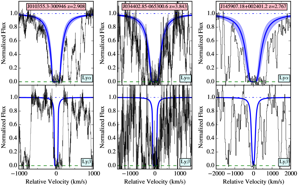
Figure 1.— H I Ly$\alpha$ (top row) and Ly$\beta$ (bottom row) profiles for three LLSs with $N_{\rm HI}\geq 10^{19}\,{\rm cm^{-2}}$. The damping wings of Ly$\alpha$ are well-resolved in these SLLSs and the blue curves indicate for the best-estimates and uncertainty of the $N_{\rm HI}$ values. These are well constrained, even in poor S/N data.

2.2. Observations

We present data obtained at the W.M. Keck and Las Campanas Observatories using the twin 10 m Keck I and Keck II telescopes and the twin 6.5 m Baade and Clay telescopes. Altogether, we used four spectrometers: (1) the High Resolution Echelle Spectrometer (HIRES; Vogt et al., 1994); (2) the Echellette Spectrograph and Imager (ESI; Sheinis et al., 2002); (3) the Magellan Inamori Kyocera Echelle (MIKE; Bernstein et al., 2003); and (4) the Magellan Echellette Spectrograph (MagE; Marshall et al., 2008).

The MagE spectra were presented in Fumagalli et al. (2013) and we refer the reader to that manuscript for details on the observations and data reduction. Similarly the ESI observations have been published previously in a series of papers (Prochaska et al., 2003b, 2007; O’Meara et al., 2007; Rafelski et al., 2012).

Observing logs for the HIRES and MIKE spectra are provided in Tables 1 and 2. A significant fraction of these data have been analyzed previously (e.g. O’Meara et al., 2007; Faucher-Giguère et al., 2008; Neeleman et al., 2013), but not for a comprehensive LLS survey.

2.3. Data Reduction

The HIRES spectra were reduced with the HIRedux software package, primarily as part of the KODIAQ project (Lehner et al., 2014). Briefly, each spectral image was bias-subtracted, flat-fielded with pixel flats, and wavelength-calibrated with corresponding ThAr frames. The echelle orders were traced using a traditional flat-field spectral image. The sky background was subtracted with a b-spline algorithm (e.g. Bochanski et al., 2009), and the quasar flux was further traced and optimally extracted with standard techniques. These spectra were flux normalized with a high-order Legendre polynomial and co-added after weighting by the median S/N of each order. This yields an individual, wavelength-calibrated spectrum for each night of observation in the vacuum and heliocentric frame. When possible, we then combined spectra from quasars observed on multiple nights with the same instrument configuration.

Processing of the MIKE spectra used the MIRedux package now bundled within the XIDL software package. This pipeline uses algorithms similar to HIRedux. The primary difference is that the flux is estimated together with the sky using a set of b-spline models which is demanded by the short $5^{\prime\prime}$ slits employed with MIKE. In addition, these data were fluxed prior to coaddition using the reduced spectrum of a spectrophotometric standard (taken from the same night in most cases). Therefore, we provide both fluxed and normalized spectra from this instrument.

Details on the data reduction of ESI and MagE spectra are provided in previous publications (Prochaska et al., 2003b; Fumagalli et al., 2013).

All of the reduced and calibrated spectra are available on the project’s website. The Keck/HIRES spectra will also be provided in the first data release of the KODIAQ project (Lehner et al. 2015).

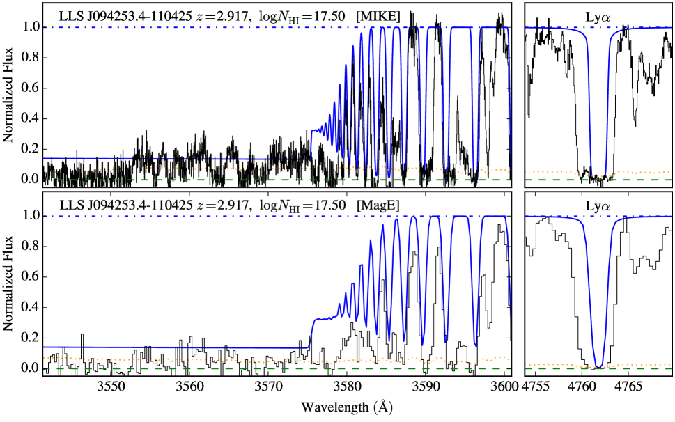
Figure 2.— Plots of the Lyman limit (left) and the Ly$\alpha$ (right) profile for the LLS at $z=2.917$ toward J0924–1104. We observed this system with both the MIKE (top) and MagE (bottom) spectrometers at LCO. The spectra show a break in the flux at $\lambda\approx 3585$Å but residual flux down to $\lambda\approx 3500$Å where the Lyman limit from a lower redshift absorber occurs. By modeling the flux decrement of the $z=2.917$ LLS, we establish a precise estimate of its total $N_{\rm HI}$ value. It is also evident that the H I Ly$\alpha$ profile alone offers very little constraint on $N_{\rm HI}$.

3. LLS Definition

Before proceeding to analysis of the sample, we strictly define the Lyman limit system. There are three aspects to the definition:

1. The velocity interval analyzed, which also corresponds to a finite redshift window.

2. The $N_{\rm HI}$ value of the system.

3. The spatial proximity of the LLS to other astrophysical objects (e.g. the background quasar or a foreground DLA).

Of these three, the first has received the least attention by the community yet may be the most important. Establishing a precise definition, however, is largely arbitrary despite the fact that it may significantly impact the studies that follow. This includes the assessment of gas kinematics (Prochaska & Wolfe, 1997), metallicity (Prochter et al., 2010; Fumagalli et al., 2011a), and even the contribution of LLSs to the cosmic mean free path (Prochaska et al., 2014b). In this paper (and future publications), we adopt an observationally-motivated velocity interval of $\pm 500{\rm km~{}s^{-1}}$ centered on the peak optical depth $z_{\rm LLS}^{\rm peak}$ of the H I Lyman series. Frequently, we estimate $z_{\rm LLS}^{\rm peak}$ from the peak optical depth of a low-ion, metal-line transition. An LLS, then, is all of the optically thick gas at $|\delta v|<500{\rm km~{}s^{-1}}$ from $z_{\rm LLS}^{\rm peak}$. In practice, we have not simply summed the H I column densities of all Ly$\alpha$ absorbers within this interval. Instead, we have adopted the integrated $N_{\rm HI}$ estimate from the Lyman limit decrement or adopt $N_{\rm HI}$ from the analysis of damping in the Ly$\alpha$ profiles (see the next section for more detail). As an example of the latter, we treat the two absorbers at $z=3.1878$ and $z=3.1917$ towards PKS2000-330 (Prochter et al., 2010) as a single LLS. Similarly, we sum metal-line absorption identified within the interval although it rarely is detected in intervals that exceeds 200km s^-1. Moreover, this window was adjusted further to exclude absorption from unrelated (e.g higher or lower redshift) systems. While this is an observationally driven definition, we note that it should also capture even the largest peculiar motions within dark matter halos at $z\sim 2$.

With $|\delta v|<500{\rm km~{}s^{-1}}$ as the first criterion, we define an LLS as any combination of systems with $N_{\rm HI}\geq 10^{17.3}\,{\rm cm^{-2}}$ within that interval; this yields an integrated optical depth at the Lyman limit $\tau_{\rm 912}\geq 1$. In practice, we distinguish the LLS from DLAs by requiring that $N_{\rm HI}<10^{20.3}\,{\rm cm^{-2}}$. Systems with $10^{16}<N_{\rm HI}<10^{17.3}\,{\rm cm^{-2}}$ are referred to as partial LLSs or pLLSs, and are excluded from analysis in this manuscript. Last, we refer to an LLS within 3000 km s^-1 of the background quasar as a proximate LLS or PLLS (Prochaska et al., 2008b). There are 5 PLLSs within our sample satisfying this definition, all with velocity separations of at least $2000{\rm km~{}s^{-1}}$ from the reported quasar redshifts. Altogether, we present measurements for 157 LLSs at redshifts $z_{\rm LLS}=1.76-4.39$ and with $N_{\rm HI}=10^{17.3}-10^{20.25}\,{\rm cm^{-2}}$. Here and in future papers we refer to this dataset as the high-dispersion LLS sample (HD-LLS Sample). We will augment this sample in the years to follow via our web site.

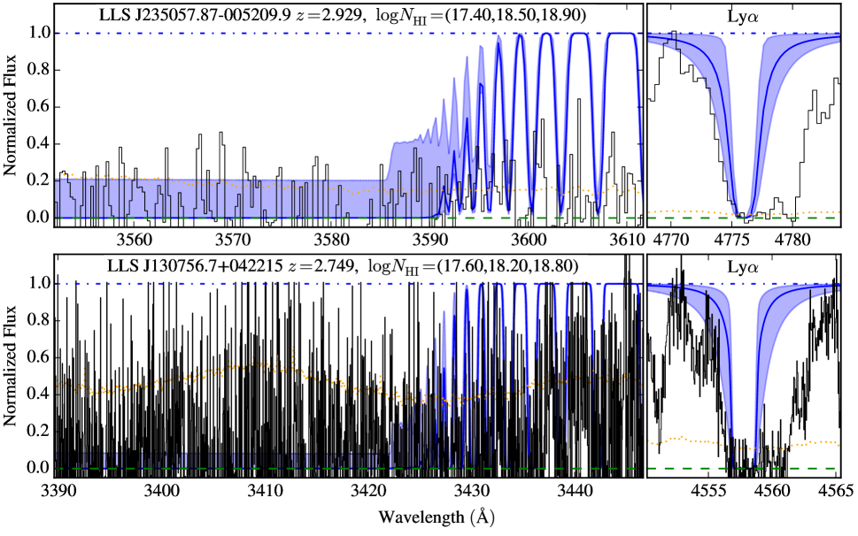
Figure 3.— Two examples of LLSs with a strong Lyman limit break ($\tau_{\rm 912}>1$) yet weak or absent damping of H I Ly$\alpha$. In these examples, we only estimate bounds on the $N_{\rm HI}$ values which can span an order-of-magnitude uncertainty.

4. $N_{\rm HI}$ Analysis

Although the continuum opacity of the Lyman limit generates an unambiguous signature in a quasar spectrum, it is generally challenging to precisely estimate the H I column density $N_{\rm HI}$ for a given LLS system. This follows simply from the fact that $\exp(-\tau_{\rm 912})\ll 1$ for $N_{\rm HI}>10^{18}\,{\rm cm^{-2}}$ and all of the H I Lyman series lines are on the saturated portion of the curve-of-growth for $N_{\rm HI}<10^{19}\,{\rm cm^{-2}}$. Furthermore, the damping of Ly$\alpha$ is difficult to measure for $N_{\rm HI}\ll 10^{20}\,{\rm cm^{-2}}$, especially in low S/N spectra or at $z>3$ where IGM blending is substantial.

Our approach to identifying LLS and estimating their $N_{\rm HI}$ values involved two relatively distinct procedures. For LLS with large $N_{\rm HI}$ values ($>10^{19}\,{\rm cm^{-2}}$), we searched each spectrum for absorption features with large equivalent widths $W_{\lambda}$ characteristic of a damped Ly$\alpha$ line (i.e. $W_{\lambda}\gg 1$Å). We then considered whether these candidates could be related to a broad absorption line (BAL) system associated to the background quasar or Ly$\beta$ associated to a higher redshift DLA. Any such coincidences were eliminated. For the remaining candidates, we performed an analysis of the Ly$\alpha$ profile by overplotting a series of Voigt profiles with $N_{\rm HI}>10^{18.5}\,{\rm cm^{-2}}$, adjusting the local continuum by-eye as warranted. When low-ion metal absorption was detected near the approximate centroid of Ly$\alpha$, we centered the model to its peak optical depth and refined the $N_{\rm HI}$ value accordingly. We did not, however, require the positive detection of metal-line absorption. In all cases, the Doppler parameter of the model Ly$\alpha$ line was set to 30 km s^-1.

For cases were the S/N was deemed sufficient and line-blending not too severe, we estimated (by visual inspection) a ‘best’ $N_{\rm HI}$ value and corresponding $1\sigma$ uncertainties. Although this procedure is rife with human interaction, we maintain that it offers the most robust assessment (to date) for $N_{\rm HI}$ estimation. This is because the dominant uncertainties are systematic (e.g. continuum placement and line-blending), which are difficult to estimate statistically. Figure 1 shows three examples of LLSs with damped Ly$\alpha$ lines giving precisely estimated $N_{\rm HI}$ values. Such systems are commonly referred to as super LLSs (SLLSs) or sub-DLAs.

Table 3$N_{\rm HI}$ ESTIMATES FOR THE HD-LLS SAMPLE

Quasar	$z_{\rm peak}^{a}$	$N_{\rm HI}^{\rm low}$	$N_{\rm HI}^{\rm high}$	$N_{\rm HI}^{\rm adopt}$	$flg_{\rm HI}^{b}$
J1608+0715	1.7626	19.10	19.70	$19.40_{-0.30}^{+0.30}$	1
J0953+5230	1.7678	20.00	20.20	$20.10_{-0.10}^{+0.10}$	1
J0927+5621	1.7749	18.90	19.10	$19.00_{-0.10}^{+0.10}$	1
J1509+1113	1.8210	18.00	19.00	$18.50_{-0.50}^{+0.50}$	2
J101939.15+524627	1.8339	18.80	19.40	$19.10_{-0.30}^{+0.30}$	1
Q1100-264	1.8389	19.25	19.55	$19.40_{-0.15}^{+0.15}$	1
J1159-0032	1.9044	19.90	20.20	$20.05_{-0.15}^{+0.15}$	1
Q0201+36	1.9548	19.90	20.30	$20.10_{-0.20}^{+0.20}$	1
J0828+0858	2.0438	19.80	20.00	$19.90_{-0.10}^{+0.10}$	1
J2123-0050	2.0593	19.10	19.40	$19.25_{-0.15}^{+0.15}$	1
Q1456-1938	2.1701	19.55	19.95	$19.75_{-0.20}^{+0.20}$	1
J034024.57-051909	2.1736	19.15	19.55	$19.35_{-0.20}^{+0.20}$	1
Q0001-2340	2.1871	19.50	19.80	$19.65_{-0.15}^{+0.15}$	1
SDSS1307+0422	2.2499	19.85	20.15	$20.00_{-0.15}^{+0.15}$	1
J1712+5755	2.3148	20.05	20.35	$20.20_{-0.15}^{+0.15}$	1
Q2053-3546	2.3320	18.75	19.25	$19.00_{-0.25}^{+0.25}$	1
Q2053-3546	2.3502	19.35	19.85	$19.60_{-0.25}^{+0.25}$	1
Q1456-1938	2.3512	19.35	19.75	$19.55_{-0.20}^{+0.20}$	1
J1131+6044	2.3620	19.90	20.20	$20.05_{-0.15}^{+0.15}$	1
Q1206+1155	2.3630	20.05	20.45	$20.25_{-0.20}^{+0.20}$	1
HE2314-3405	2.3860	18.80	19.20	$19.00_{-0.20}^{+0.20}$	1
Q0301-005	2.4432	19.75	20.05	$19.90_{-0.15}^{+0.15}$	1
HS1345+2832	2.4477	19.70	20.00	$19.85_{-0.15}^{+0.15}$	1
J1035+5440	2.4570	19.40	19.90	$19.65_{-0.25}^{+0.25}$	1
Q1337+11	2.5080	20.00	20.30	$20.15_{-0.15}^{+0.15}$	1
SDSS0912+0547	2.5220	19.15	19.55	$19.35_{-0.20}^{+0.20}$	1
SDSS0209-0005	2.5228	18.90	19.20	$19.05_{-0.15}^{+0.15}$	1
LB1213+0922	2.5230	20.00	20.40	$20.20_{-0.20}^{+0.20}$	1
Q0207-003	2.5231	18.80	19.20	$19.00_{-0.20}^{+0.20}$	1
Q0207-003	2.5466	17.60	18.60	$18.10_{-0.50}^{+0.50}$	2
HS1104+0452	2.6014	19.70	20.10	$19.90_{-0.20}^{+0.20}$	1
J2234+0057	2.6040	19.25	19.75	$19.50_{-0.25}^{+0.25}$	1
J115659.59+551308.1	2.6159	18.80	19.30	$19.10_{-0.30}^{+0.30}$	1
SDSS1558-0031	2.6300	19.40	19.75	$19.60_{-0.20}^{+0.20}$	1
SDSS0157-0106	2.6313	19.25	19.65	$19.45_{-0.20}^{+0.20}$	1
Q2126-158	2.6380	19.10	19.40	$19.25_{-0.15}^{+0.15}$	1
Q1455+123	2.6481	17.30	19.40	$18.35_{-1.05}^{+1.05}$	2
LBQS2231-0015	2.6520	18.70	19.30	$19.10_{-0.40}^{+0.20}$	1
SDSS0121+1448	2.6623	19.05	19.40	$19.25_{-0.20}^{+0.15}$	1
SDSSJ0915+0549	2.6631	17.50	18.90	$18.20_{-0.70}^{+0.70}$	2
SDSSJ2319-1040	2.6750	19.30	19.60	$19.45_{-0.15}^{+0.15}$	1
Q0201+36	2.6900	17.50	18.80	$18.50_{-1.00}^{+0.30}$	2
LB2203-1833	2.6981	19.85	20.15	$20.00_{-0.15}^{+0.15}$	1
SDSSJ1551+0908	2.7000	17.30	17.70	$17.50_{-0.20}^{+0.20}$	1
HS1200+1539	2.7080	17.60	18.90	$18.30_{-0.70}^{+0.70}$	2
Q1508+087	2.7219	19.00	19.80	$19.40_{-0.40}^{+0.40}$	1
PMNJ1837-5848	2.7289	17.50	18.70	$18.10_{-0.60}^{+0.60}$	2

Note. — All column densities are log₁₀. The flag in the final column indicates the quality of the measurement. A $flg_{\rm HI}=1$ corresponds to a more precisely measured value and one may assume a Gaussian PDF with the errors reported taken as $1\sigma$ uncertainties. A $flg_{\rm HI}=2$ corresponds to a less precisely measured value, and we recommend one adopt a uniform prior for $N_{\rm HI}$ within the error interval reported. See text for further details.

We provide the adopted $N_{\rm HI}$ values and error estimates of our SLLS sample (99 systems with $N_{\rm HI}\geq 10^{19}\,{\rm cm^{-2}}$) in Table 3. These represent roughly 2/3 of the total HD-LLS Sample. This high fraction occurs because we only require coverage of H I Ly$\alpha$ to identify and analyze these SLLS. This implies a much larger survey path-length than for the lower $N_{\rm HI}$ LLS. In addition, one may identify and analyze multiple SLLSs along a given sightline whereas one is restricted to a single LLS when the Lyman Limit is central to the analysis. Because these SLLSs tend to span nearly the entire $\pm 500{\rm km~{}s^{-1}}$ window that defines an LLS, it is possible that there is additional, optically thick gas not included in our $N_{\rm HI}$ estimate. This will be rare, however, and the underestimate of $N_{\rm HI}$ should generally be much less than 10%.

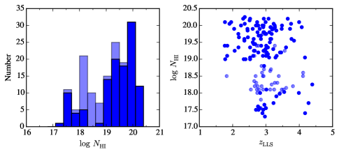
Figure 4.— (left) Histogram of $N_{\rm HI}$ values for the HD-LLS Sample. The ligher bars indicate $N_{\rm HI}$ values with large uncertainty ($1\sigma>0.4$ dex). Nearly two-thirds of the sample have $N_{\rm HI}\geq 10^{19}\,{\rm cm^{-2}}$ which is a consequence of the spectral coverage required to estimate $N_{\rm HI}$ for an LLS (see text). (right) Scatter plot of $N_{\rm HI}$ vs. $z_{\rm LLS}$ for the sample. Again, the lighter points indicate LLSs with poorer constraints on the $N_{\rm HI}$ values (flg=2 in Table 3). Systems with $N_{\rm HI}<10^{19}\,{\rm cm^{-2}}$ all have $z_{\rm LLS}>2.6$ as coverage of the Lyman limit is required for the H I analysis.

In parallel with the search for LLSs having strong Ly$\alpha$ lines, we inspected each spectrum for a Lyman limit break. For those the LLSs that exhibit non-negligible flux at the Lyman limit, i.e. $\tau_{\rm 912}<3$, a precise $N_{\rm HI}$ estimation may be recovered. In practice, such analysis is hampered by poor sky subtraction and associated IGM absorption that stochastically reduces the quasar flux through the spectral region near the Lyman limit and affects continuum placement. In the following, we have been conservative regarding the systems with $N_{\rm HI}$ measurements from the Lyman limit flux decrement. We are currently acquiring additional, low-dispersion spectra to confirm the flux at the Lyman limit for a set of the HD-LLS Sample. Figure 2 shows one example of a pLLS observed with both the MIKE and MagE spectrometers. The flux decrement is obvious and one also appreciates the value of higher spectral resolution (with high S/N) for resolving IGM absorption.

For the remainder of the systems identified on the basis of a Lyman limit break, we adopt conservative bounds (i.e. upper and lower limits) to the $N_{\rm HI}$ values. These are based primarily on analysis of the Ly$\alpha$ line and the flux at the Lyman limit. The absence of strong damping in the former provides a strict upper limit to $N_{\rm HI}$ while the latter sets a firm lower limit. These bounds are provided in Table 3, and Figure 3 shows two examples of these ‘ambiguous’ cases. In practice, the bounds are often an order-of-magnitude apart, e.g. $10^{17.7}\,{\rm cm^{-2}}<N_{\rm HI}<10^{18.9}\,{\rm cm^{-2}}$. Furthermore, it is difficult to estimate the probability distribution function (PDF) of $N_{\rm HI}$ within these bounds. One should not, for example, assume a Gaussian PDF centered within the bounds with a dispersion of half the interval. In fact, we expect that the PDF is much closer to uniform, i.e. equal probability for any $N_{\rm HI}$ value within the bounds. This expectation is motivated by current estimations of the $N_{\rm HI}$ frequency distribution $f(N_{\rm HI},X)$ which argue for a uniform distribution of $N_{\rm HI}$ values for randomly selected systems with $N_{\rm HI}\approx 10^{18}\,{\rm cm^{-2}}$ (Prochaska et al., 2010; O’Meara et al., 2013). Going forward, we advocate adopting a uniform PDF.

As a cross-check on the analysis, 50 of the sightlines were re-analyzed by a second author to identify LLSs and estimate their $N_{\rm HI}$ values. With two exceptions, the values between the two authors agree within the estimated uncertainty and we identify no obvious systematic bias. These two exceptions have $>0.5$ dex difference due to differing definitions used by the two authors and we have adopted the values corresponding to the strict definition provided in $\S$ 3. This exercise confirms that the uncertainties are dominated by systematic effects, not S/N nor the analysis procedures.

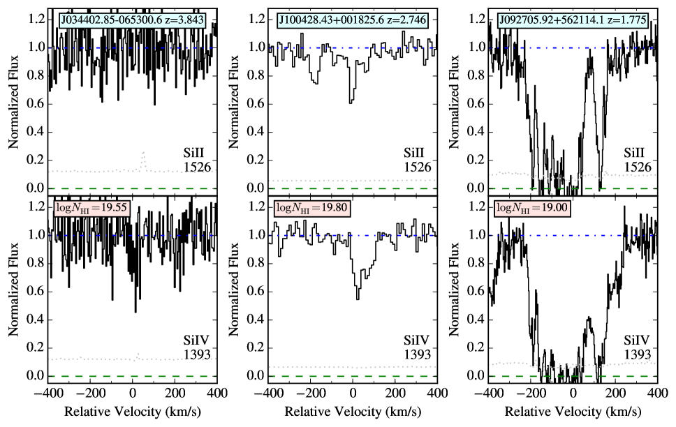
Figure 5.— Si II and Si IV transitions for three SLLS representative of the full HD-LLS Sample. Note the large diversity in metal-line strength despite the comparable $N_{\rm HI}$ values. These systems have a tendency to show both low and high-ion absorption indicative of partially ionized gas. The gray dotted line in each panel indicates the estimated $1\sigma$ error array.

Table 4IONIC COLUMN SUMMARY FOR Si AND C

Quasar	$z_{\rm abs}$	$N_{\rm HI}$	${N({\rm C^{+}})}$	$\sigma({N({\rm C^{+}})})$	${N({\rm C^{3+}})}$	$\sigma({N({\rm C^{3+}})})$	${N({\rm Si^{+}})}$	$\sigma({N({\rm Si^{+}})})$	${N({\rm Si^{3+}})}$	$\sigma({N({\rm Si^{3+}})})$
J1608+0715	1.7626	$19.40_{-0.30}^{+0.30}$					15.80	-9.99
J0953+5230	1.7678	$20.10_{-0.10}^{+0.10}$	15.44	+9.99	15.21	+9.99	15.67	0.01	14.57	+9.99
J0927+5621	1.7749	$19.00_{-0.10}^{+0.10}$	15.40	+9.99	15.40	+9.99	15.58	0.02	14.84	+9.99
J1509+1113	1.8210	$18.50_{-0.50}^{+0.50}$			14.83	+9.99	14.21	0.04	14.17	+9.99
J101939.15+524627	1.8339	$19.10_{-0.30}^{+0.30}$			14.93	+9.99	15.32	0.03	14.14	+9.99
Q1100-264	1.8389	$19.40_{-0.15}^{+0.15}$			14.24	0.00	13.96	0.01	13.83	0.00
J1159-0032	1.9044	$20.05_{-0.15}^{+0.15}$	15.38	+9.99	15.22	+9.99	15.14	0.10	14.54	+9.99
Q0201+36	1.9548	$20.10_{-0.20}^{+0.20}$					15.11	0.09
J0828+0858	2.0438	$19.90_{-0.10}^{+0.10}$	15.14	+9.99	14.89	+9.99	15.25	0.10	14.44	+9.99
J2123-0050	2.0593	$19.25_{-0.15}^{+0.15}$	15.11	+9.99	14.60	+9.99	14.60	0.04	13.96	0.00
Q1456-1938	2.1701	$19.75_{-0.20}^{+0.20}$					14.84	-9.99
J034024.57-051909	2.1736	$19.35_{-0.20}^{+0.20}$	14.40	+9.99	13.86	0.02	13.84	0.02	13.39	0.02
Q0001-2340	2.1871	$19.65_{-0.15}^{+0.15}$	14.45	+9.99	14.26	0.01	13.75	0.03	13.74	0.01
SDSS1307+0422	2.2499	$20.00_{-0.15}^{+0.15}$			14.22	0.03	14.25	+9.99
J1712+5755	2.3148	$20.20_{-0.15}^{+0.15}$			13.36	0.04	14.08	0.01

Note. — All column densities are log₁₀. When the reported $\sigma=+9.99$, the measured value should be taken as a lower limit. Similarly, $\sigma=-9.99$ indicates that the reported value refers to an upper limit at 95% c.l.

Note. — [The complete version of this table is in the electronic edition of the Journal. The printed edition contains only a sample.]

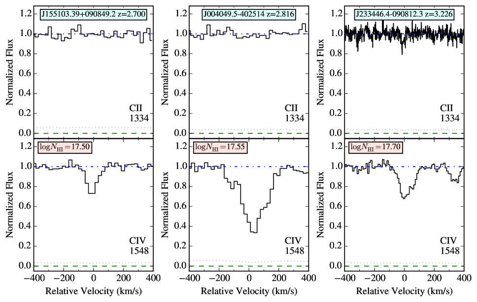
Figure 6.— C II and C IV transitions for LLSs with low $N_{\rm HI}$ values. Unlike the SLLSs from Figure 5, these LLSs have metal absorption that is dominated by high-ions. There only a few cases of LLSs with $N_{\rm HI}<10^{18}\,{\rm cm^{-2}}$ and a positive low-ion detection.

Table 5IONIC COLUMN SUMMARY FOR Al, Fe, and O

Quasar	$z_{\rm abs}$	$N_{\rm HI}$	${N({\rm O^{0}})}$	$\sigma({N({\rm O^{0}})})$	${N({\rm Al^{+}})}$	$\sigma({N({\rm Al^{+}})})$	${N({\rm Al^{++}})}$	$\sigma({N({\rm Al^{++}})})$	${N({\rm Fe^{+}})}$	$\sigma({N({\rm Fe^{+}})})$
J1608+0715	1.7626	$19.40_{-0.30}^{+0.30}$					13.53	0.00
J0953+5230	1.7678	$20.10_{-0.10}^{+0.10}$	15.68	+9.99	13.96	+9.99	13.86	0.01	14.99	0.10
J0927+5621	1.7749	$19.00_{-0.10}^{+0.10}$	15.63	+9.99	13.92	+9.99	14.05	0.01	15.28	0.13
J1509+1113	1.8210	$18.50_{-0.50}^{+0.50}$			13.12	+9.99	13.04	0.05	13.76	0.11
J101939.15+524627	1.8339	$19.10_{-0.30}^{+0.30}$			13.34	+9.99	13.62	0.02	14.19	0.02
Q1100-264	1.8389	$19.40_{-0.15}^{+0.15}$			12.79	0.01	12.31	0.10	13.42	0.01
J1159-0032	1.9044	$20.05_{-0.15}^{+0.15}$	15.66	+9.99	13.98	+9.99	13.82	0.01
Q0201+36	1.9548	$20.10_{-0.20}^{+0.20}$			13.77	+9.99	13.61	0.01
J0828+0858	2.0438	$19.90_{-0.10}^{+0.10}$	15.49	+9.99			13.59	0.02	14.89	0.04
J2123-0050	2.0593	$19.25_{-0.15}^{+0.15}$			13.44	+9.99	13.15	0.01	14.39	0.00
Q1456-1938	2.1701	$19.75_{-0.20}^{+0.20}$			13.38	+9.99	12.99	0.04	14.26	0.01
J034024.57-051909	2.1736	$19.35_{-0.20}^{+0.20}$	14.56	+9.99	12.65	0.03	12.49	0.14
Q0001-2340	2.1871	$19.65_{-0.15}^{+0.15}$	14.16	0.04	13.00	+9.99	12.40	-9.99	13.11	0.03
SDSS1307+0422	2.2499	$20.00_{-0.15}^{+0.15}$			13.04	+9.99	12.80	0.07	14.18	0.04
J1712+5755	2.3148	$20.20_{-0.15}^{+0.15}$			12.56	0.02	12.39	0.06	13.65	0.03

Note. — All column densities are log₁₀. When the reported $\sigma=+9.99$, the measured value should be taken as a lower limit. Similarly, $\sigma=-9.99$ indicates that the reported value refers to an upper limit at 95% c.l.

Note. — [The complete version of this table is in the electronic edition of the Journal. The printed edition contains only a sample.]

Table 3 lists the adopted $N_{\rm HI}$ value, errors on this value, the bounds on $N_{\rm HI}$, and a flag indicating whether one would assume a normal or uniform PDF. Figure 4 shows a histogram of the adopted $N_{\rm HI}$ values and a scatter plot against $z_{\rm LLS}$. It is evident that the HD-LLS Sample is weighted towards higher $N_{\rm HI}$ values and $z\sim 3$.

5. Ionic Column Densities

For each of the HD-LLS Sample, we inspected the spectra for associated metal-line absorption. Emphasis was placed on transitions with observed wavelengths redward of the Ly$\alpha$ forest. A velocity interval was estimated for the column density measurements based on the cohort of transitions detected. Velocity plots were generated and inspected to search for line-blending. Severely blended lines were eliminated from analysis and intermediate/weak cases were measured but reported as upper limits. All of these assignments were vetted by JXP, MF, and JMO. Figures 5 and 6 show the Si II 1526/Si IV 1393 transitions for three representative SLLSs and the C II 1334/C IV 1548 transitions for three LLSs with $N_{\rm HI}\lesssim 10^{17.7}\,{\rm cm^{-2}}$. These data indicate a great diversity of line-strengths for these transitions within the SLLS sample. We also conclude that metal-absorption is dominated by high-ions in the lower $N_{\rm HI}$ systems.

Column densities were measured using the apparent optical depth method (AODM; Savage & Sembach, 1991) which gives accurate results for unsaturated line profiles. On the latter point, the echelle data (MIKE,HIRES) have sufficiently high resolution to directly assess line-saturation, i.e. only profiles with minimum normalized flux $f_{\rm min}$ less than 0.1 may be saturated. For the echellette data (MagE, ESI), however, line-saturation is a concern (e.g. Prochaska et al., 2003b). In general, we have proceeded conservatively by treating most lines as saturated when $f_{\rm min}<0.5$. For many of the ions analyzed in these LLSs, we observe multiple transitions with differing oscillator strengths and have further assessed line-saturation from the cohort of measurements.

Uncertainties were estimated from standard propagation of error, which does not include error from continuum placement. To be conservative, we adopt a minimum uncertainty of 0.05 dex to the measurements from a given transition. When multiple transitions from the same ion were measured (e.g. Si II 1304 and Si II 1526 for Si⁺), we calculate the ionic column density from the weighted mean. Otherwise, we adopt the measurement from the single transition or a limit from the cohort emphasizing positive detections.

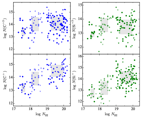
Figure 7.— Scatter plot of Si and C ionic column densities for the HD-LLS Sample. Circles indicate measured values; their uncertainties are generally less than 0.1 dex. Triangles indicate limits to the values with the open symbols indicating upper limits. Lighter points mark LLSs with a poorly constrained $N_{\rm HI}$ value. Gray boxes encompass 50-percent of the measurements in three logarithmic $N_{\rm HI}$ intervals: [17.3, 18.0), [18.0, 19.0), [19.0, 20.3). At all column densities, there is a large dispersion in the measurements. Nevertheless, the low-ions (C⁺, Si⁺) exhibit a strong, positive correlation with $N_{\rm HI}$ value. A Spearman rank test rules out the null hypothesis at $>99.99\%$ c.l.

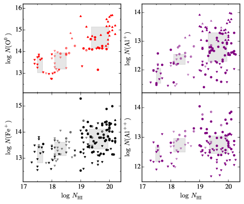
Figure 8.— Same as Figure 7 but for four additional ions.

A complete set of tables and figures for the metal-line transitions analyzed for each LLS are given online. Tables 4 and 5 summarize the results for Al⁺, Al⁺⁺, Fe⁺, C⁺, C⁺³, O⁰, Si⁺, and Si⁺³. A listing of all the measurements from this manuscript is provided in the Appendix. Figures 7 and 8 show the column density distributions for a set of Al, Fe, Si, C, and O atoms/ions as a function of the LLS $N_{\rm HI}$ value. Not surprisingly, the lower ionization states show an obvious correlation with H I column density although there is a large scatter at all values. The near absence of positive detections for O I (i.e. ${N({\rm O^{0}})}<10^{14}\,{\rm cm^{-2}}$) at low $N_{\rm HI}$ is also notable. This suggests a rarity of high metallicity gas in systems with $\tau_{\rm 912}<10$. The high ions are also positively correlated with the neutral column but with yet larger scatter and much smaller correlation coefficients.

6. Results

In the following, we present a set of results derived from the column density measurements of the previous sections. For this manuscript, we restrict the analysis to an empirical investigation. Future studies will introduce additional models and analysis (e.g. photoionization modeling) to interpret the data. We further restrict the discussion to ionic abundances and defer the analysis of kinematics to future work.

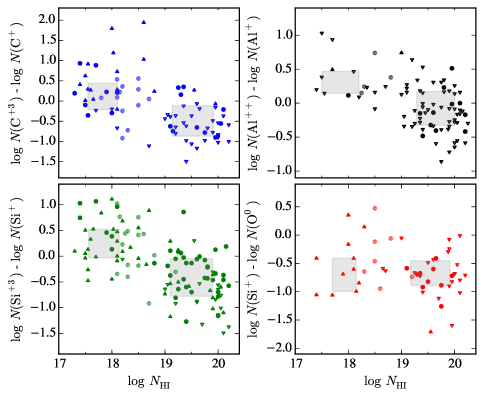
Figure 9.— Scatter plots of four ionic ratios that diagnose the ionization state of the LLSs. Gray boxes encompass 50-percent of the measurements in two logarithmic $N_{\rm HI}$ intervals: [17.3, 19.0), [19.0, 20.3). The C, Si, and Al ratios show strong evidence that the gas is more highly ionized at low $N_{\rm HI}$ values. Similarly, the set of Si⁺/O⁰ values exceeding $-0.7$ dex are indicative of a highly ionized gas. We further emphasize that the $\log({\rm Si^{+}}/{\rm Si^{+3}})\approx-0.5$ dex values at high $N_{\rm HI}$ suggests that this gas is also partially ionized.

6.1. Ionization State

As noted above, a full treatment of the ionization state of the gas including the comparison to models will be presented in a future manuscript. We may, however, explore the state of the gas empirically through the examination of ionic ratios that are sensitive to the ionization state of the gas. Figure 9 presents four such ionic ratios against $N_{\rm HI}$. These primarily compare ions of the same element (e.g. C⁺³/C⁺) to eliminate offsets due to differing intrinsic chemical abundances (i.e. varying abundance ratios). In this analysis, we have taken the integrated column density across the entire LLS. While there is evidence for variations in these ratios within individual components, these tend to be small (e.g. Prochter et al., 2010, Figure 5). Therefore, the trends apparent in Figure 9 reflect the gross properties of the LLS sample.

All of the C⁺³/C⁺, Si⁺³/Si⁺, and Al⁺⁺/Al⁺ ratios exhibit a strong anti-correlation with $N_{\rm HI}$ indicating an increasing neutral fraction with increasing H I opacity. Taking limits as values, the Spearman rank test yields a probability of less than $10^{-3}$ for the null hypothesis, in each case. For all of these ions, the upper ionization state is dominant for $N_{\rm HI}\lesssim 10^{18.5}\,{\rm cm^{-2}}$ and vice-versa for higher $N_{\rm HI}$ values. We emphasize, however, that even at $N_{\rm HI}\approx 10^{20}\,{\rm cm^{-2}}$ the observed ratios are frequently large, e.g. $\log({\rm Si^{+3}/Si^{+}})\approx-0.5$ dex. This suggests that the gas is predominantly ionized even at these larger total H I opacities.

This inference is further supported by the Si⁺/O⁰. Ignoring differential depletion, which we expect to be modest in LLSs, the Si⁺/O⁰ ratio should trend towards the solar abundance ratio ($\epsilon_{\rm Si}/\epsilon_{\rm O}=-1.2$ dex) in a neutral gas given that Si and O are both produced in massive stars and are observed to trace each other in astrophysical systems (e.g. stellar atmospheres). We identify, however, a significant sample of systems with $N_{\rm HI}\approx 10^{18.5}\,{\rm cm^{-2}}$ that have $\log({\rm Si^{+}/O^{0}})>-1$ dex. Because the majority of ionization processes (e.g. photoionization, collisional ionization) predict ${\rm Si^{+}/O^{0}}>$ Si/O (e.g. Prochaska & Hennawi, 2009), these measurements offer further evidence that LLSs are highly ionized.

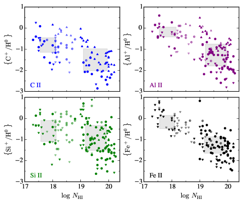
Figure 10.— Scatter plots of low-ion column densities relative to H I, normalized to the solar abundance $\{{\rm X}^{i}/{\rm H}^{0}\}$ and plotted against the LLS $N_{\rm HI}$ value. Gray boxes encompass 50-percent of the measurements in two logarithmic $N_{\rm HI}$ intervals: [17.3, 19.0), [19.0, 20.3). If ionization corrections are small, $\{{\rm X}^{i}/{\rm H}^{0}\}$ provides an estimate of the logarithmic metal abundance relative to solar. The measurements appear to indicate a declining trend of gas metallicity with increasing $N_{\rm HI}$. We argue, however, that this apparent trend is driven by ionization effects and the set of upper/lower limits at low/high $N_{\rm HI}$ values. Furthermore, given the large scatter at all $N_{\rm HI}$ values, it will be challenging to establish any trend between enrichment and $N_{\rm HI}$ value in the LLSs.

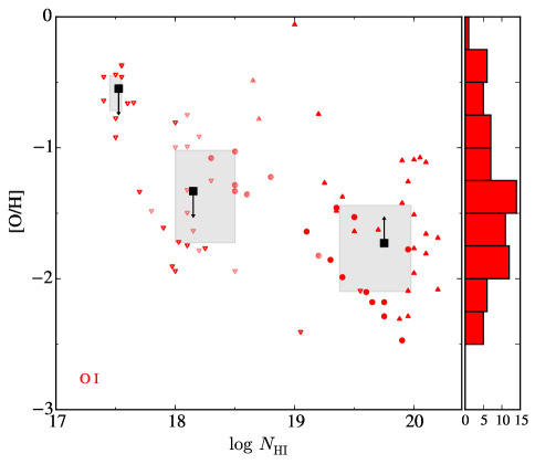
Figure 11.— Estimations of the oxygen metallicity in the LLSs where we have assumed that [O/H]=$\{{\rm O}^{0}/{\rm H}^{0}\}$, i.e. that ionization corrections are small for this ionic ratio (see the text). Gray boxes encompass 50-percent of the measurements in three logarithmic $N_{\rm HI}$ intervals: [17.3, 18.0), [18.0, 19.0), [19.0, 20.3). Similar to the results for other low-ions (Figure 10), there is an apparent decline in [O/H] with $N_{\rm HI}$. This apparent trend, however, is primarily driven by the high incidence of upper/lower limits at low/high $N_{\rm HI}$ values. In fact, the underlying trend may well be the opposite. Compare the set of low [O/H] values and upper limits at $N_{\rm HI}\approx 10^{18}\,{\rm cm^{-2}}$ with the large set of lower limits at $N_{\rm HI}\approx 10^{19.7}\,{\rm cm^{-2}}$.

6.2. Metallicity

A principal diagnostic of the LLSs is the gas metallicity, i.e. the enrichment of the gas in heavy elements. This quantity is generally characterized relative to the chemical abundances observed for the Sun. For the following, we adopt the solar abundance scale compiled by Asplund et al. (2009), taking meteoritic values when possible.

Because the LLSs are significantly ionized, the observed ionic abundances reflect only a fraction of the total abundances of Si, O, H, etc. Therefore, a full treatment requires ionization modeling. We may, however, offer insight into the problem by examining several ions relative to H⁰. To minimize ionization corrections, one restricts the analysis to ionization states dominant in a highly optically thick (i.e. neutral) medium.

The results for four low-ions are presented in Figure 10, normalized to the solar abundance. We have introduced here a new quantity and notation: $\{{\rm X}^{i}/{\rm Y}^{j}\}$ $\equiv\log({N({\rm X^{i}})}/{N({\rm Y^{j}})})-\epsilon_{\rm X}+\epsilon_{\rm Y}$, where $\epsilon_{\rm X}$ is the solar abundance on the logarithmic scale for element X. This quantity explicitly ignores ionization corrections and should not be considered a proper estimate of the chemical abundance ratio, traditionally expressed as [X/Y]. In the cases where ionization corrections are negligible, however, $\{{\rm X}^{i}/{\rm H}^{0}\}$ = [X/H] and this quantity represents the metallicity.

A cursory inspection of the plots suggests a significant decline in metal content with increasing $N_{\rm HI}$. This apparent anti-correlation, however, is driven by at least two factors. First, larger $N_{\rm HI}$ implies larger metal column densities such that the transitions saturate yielding a preponderance of lower limits. By the same token, at low $N_{\rm HI}$ values the transitions are often undetected yielding upper limits to the ionic ratios. Second, we have argued from Figure 9 that the gas is increasingly ionized with decreasing $N_{\rm HI}$. For Si⁺, C⁺, and Al⁺, the ionization corrections for $\{{\rm X}^{i}/{\rm H}^{0}\}$ are likely negative (e.g. Prochaska, 1999; Fumagalli et al., 2011a), and would lower the metallicity one infers from such ratios. We believe these factors dominate the trends apparent in Figure 10.

In fact, it is even possible that the true distribution exhibits the opposite trend. Figure 11 shows [O/H] against $N_{\rm HI}$ for the LLSs where we have assumed no ionization corrections, i.e. [O/H] = $\{{\rm O}^{0}/{\rm H}^{0}\}$. This approximation is justified by the fact that O⁰ and H⁰ have very similar ionization potentials and their neutral states are coupled by charge-exchange reactions. This assumption may break down at low $N_{\rm HI}$ values in the presence of a hard radiation field (Sofia & Jenkins, 1998; Prochter et al., 2010), but the corrections are still likely to be modest (several tenths dex). Unfortunately, the measurements are dominated by limits: upper limits at $N_{\rm HI}<10^{18.5}\,{\rm cm^{-2}}$ and lower limits at $N_{\rm HI}>10^{19}\,{\rm cm^{-2}}$. Nevertheless, the data require that [O/H] $>-1.7$ for the SLLSs and indicate [O/H] $<-1.3$ dex for LLSs with $N_{\rm HI}\approx 10^{18}\,{\rm cm^{-2}}$. We tentatively infer that the median metallicity is approximately flat with $N_{\rm HI}$ and possibly increasing; more strictly, we rule out a steeply declining O/H metallicity with increasing $N_{\rm HI}$. A similar conclusion may be drawn from the $\{{\rm Si}^{+}/{\rm H}^{0}\}$ measurements which scatter less from line-saturation. The LLSs with $N_{\rm HI}\approx 10^{18}\,{\rm cm^{-2}}$ show very few positive detections and have a median $\{{\rm Si}^{+}/{\rm H}^{0}\}$ $<-1$ dex. In contrast, the LLSs at $N_{\rm HI}\approx 10^{19.5}\,{\rm cm^{-2}}$ frequently exhibit $\{{\rm Si}^{+}/{\rm H}^{0}\}$ $>-1$ dex.

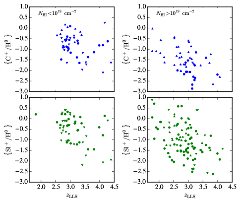
Figure 12.— Comparison of $\{{\rm X}^{i}/{\rm H}^{0}\}$ measurements for C⁺ and Si⁺ against absorption redshift. Left-hand panels are for the LLSs with $N_{\rm HI}<10^{19}\,{\rm cm^{-2}}$ and the right-hand panels are for the SLLS population. All of the data show evidence for a declining enrichment with increasing redshift, although this assertion is statistically significant ($>99\%$ c.l.) only for the SLLS sample. The absence of low values at $z\approx 2$ implies a reduced incidence of near-pristine gas with high H I columns at that epoch.

Another result apparent from Figure 10 is the large dispersion in measurements at every $N_{\rm HI}$ value. This is most notable for Si⁺ which has multiple transitions that permit measurements of the column density over a larger dynamic range. At the largest $N_{\rm HI}$ values, the values/limits of $\{{\rm Si}^{+}/{\rm H}^{0}\}$ span nearly four orders of magnitude! And although the measurements for LLSs with $N_{\rm HI}\approx 10^{17.5}-10^{19}\,{\rm cm^{-2}}$ include many upper limits, one identifies values and upper limits with $\{{\rm Si}^{+}/{\rm H}^{0}\}$ $>-0.5$ dex together with upper limits having $\{{\rm Si}^{+}/{\rm H}^{0}\}$ $<-2$. Clearly, any underlying trend of enrichment with $N_{\rm HI}$ will be diluted by the large intrinsic scatter within the LLSs. One may even argue that if such a dispersion is indicative of multiple astrophysical systems, then defining a mean of the LLS population has limited scientific value.

Despite the large dispersion, we emphasize that very few of the LLS in the HD-LLS Sample are “metal-free”, i.e. exhibiting no metal-line absorption and therefore consistent with primordial abundances. Of the $n_{\rm LLS}$ LLSs, only 25 have no low-ion detections outside the Ly$\alpha$ forest and 18 of these exhibit a positive detection in a higher-ion. For the other 7, one has been previously been identified as consistent with primordial (Fumagalli et al., 2011a). The remainder have a diversity of S/N and spectral coverage and therefore are generally less sensitive to measuring a low metallicity. Several will be examined in greater detail in a future manuscript. Nevertheless, we may conclude that the incidence of very low metallicity gas ($<1/1000$ solar) is rare in the LLS population ($<5\%$). Furthermore, none of the 82 LLSs with $N_{\rm HI}>10^{19.2}\,{\rm cm^{-2}}$ are metal-free. By $z\sim 3$, gas that is dense enough to exhibit a very high Lyman limit opacity has previously been polluted by heavy elements.

At the opposite end of the enrichment distribution, we identify 13 systems with a positive $\{{\rm Si}^{+}/{\rm H}^{0}\}$ measurement that exceeds 0 dex. This includes four extreme examples with $\{{\rm Si}^{+}/{\rm H}^{0}\}$ $>+0.5$ dex. Because these four LLSs also have $N_{\rm HI}\geq 10^{19}\,{\rm cm^{-2}}$ we expect that corrections for ionization are modest (see Prochaska et al., 2006) and that these are truly super-solar abundances. The others, however, have uncertainties consistent with the gas being sub-solar even before accounting for ionization. We conclude, subject to additional future analysis, that super-solar enrichment is also rare in the LLSs.

In Figure 12, we examine $\{{\rm Si}^{+}/{\rm H}^{0}\}$ and $\{{\rm C}^{+}/{\rm H}^{0}\}$ values as a function of redshift, splitting the LLS sample at $N_{\rm HI}=10^{19}\,{\rm cm^{-2}}$. The values for the lower $N_{\rm HI}$ systems suggest a declining trend with increasing redshift, e.g. in contrast to the lower redshift systems, none of the $z>3.5$ LLSs have a positive detection of $\{{\rm C}^{+}/{\rm H}^{0}\}$ $>-0.5$ dex. Even if we restrict analysis to positive detections, however, an anti-correlation is not statistically significant.

Turning to the SLLS population, the $\{{\rm X}^{i}/{\rm H}^{0}\}$ distributions show obvious trends with redshift (limits not withstanding). Treating all of the positive detections at their plotted values, a Spearman’s rank correlation test rules out the null hypothesis at $>99\%$ c.l. We interpret this anti-correlation as lower average enrichment within the SLLS at higher redshift. This conclusion relies on the assumption that ionization corrections will not evolve significantly with redshift, which will be investigated in a future work. A similar decline in metallicity has been established in the DLA population (e.g. Prochaska et al., 2003a; Rafelski et al., 2012) and has been interpeted as resulting from the ongoing enrichment of galactic ISM with cosmic time. Future work will perform a quantitative comparison between the two populations and explore the implications for the evolving enrichment of optically thick gas at $z>2$. In passing, we emphasize the absence of low $\{{\rm X}^{i}/{\rm H}^{0}\}$ values at $z\approx 2$ which implies a reduced incidence of near-pristine gas with high H I columns at that epoch.

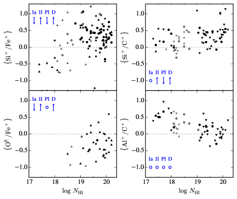
Figure 13.— Scatter plots of a series of ionic ratios, normalized to the solar relative abundances, against the $N_{\rm HI}$ values of the LLSs. The left two panels show ratios related to the $\alpha$/Fe abundance. Despite the preponderance of lower limits (especially for $\{{\rm O}^{0}/{\rm Fe}^{+}\}$), and concerns on the ionization corrections, we tentatively conclude that the LLSs exhibit super-solar $\alpha$/Fe ratios, especially at large $N_{\rm HI}$ values. The measurements in the upper-right panel indicate that Si/C is possibly enhanced by a few 0.1 dex relative to solar although the majority of the sample is consistent with [Si/C] = 0. Similarly, the $\{{\rm Al}^{+}/{\rm C}^{+}\}$ measurements are roughly consistent with the solar relative abundance or possibly sub-solar. In each panel, we indicate the expected offsets to the measurements that would be due to Type Ia (Ia) nucleosynthesis, Type II (II) nucleosynthesis, photoionization (PI), and differential depletion (D). Circles indicate a small or unknown impact.

6.3. Nucleosynthetic Patterns

It is the conventional wisdom that LLSs primarily trace gas outside of the ISM of galaxies, e.g. within their dark matter halos (aka CGM) or at yet greater distances (Fumagalli et al., 2011b; Prochaska et al., 2013). Despite their separation from galaxies, we have demonstrated that the LLSs are generally enriched in heavy elements and provided evidence that their metallicity frequently reaches $\sim 1/10$ solar abundance. Therefore, a non-negligible fraction of this optically thick medium has been processed through the furnaces of a stellar interior and presumably was transported from a galaxy via one more physical processes. One plausible transport process is an explosive event, e.g. a supernovae that expelled the gas shortly after enriching it. In this case, the gas may exhibit a distinct nucleosynthetic pattern from those observed for galactic ISM, i.e. if the supernovae ejecta did not mix prior to escaping the system. Additionally, the LLSs may couple the metal production within galaxies to the enrichment of the diffuse IGM (e.g. Aguirre et al., 2001; Schaye et al., 2003; Steidel et al., 2010). This motivates comparison of the abundances for these two diffuse and ionized phases.

We may explore several ionic ratios that trace different nucleosynthesis channels. As with metallicity, one must account for ionization effects when interpreting the results. Figure 13 plots four pairs of ions from the dataset, again represented as $\{{\rm X}^{i}/{\rm Y}^{j}\}$ with ionization corrections explicitly ignored. The figure also indicates the probable offsets to the ratios if ionization effects were important, as estimated from photoionization calculations (e.g. Prochaska 1999). Similarly, we indicate the likely offsets from differential depletion and the dominant nucleosynthesis channels (Type Ia and Type II enrichment).

The left-hand panels show two measures of $\alpha$/Fe, a key diagnostic of the relative contributions of Type Ia and Type II SNe nucleosynthesis (Tinsley, 1979). Unfortunately, the $\{{\rm O}^{0}/{\rm Fe}^{+}\}$ ratios are dominated by lower limits due to the saturation of O I 1302 and the non-detection of Fe II transitions. The values are nearly consistent with a solar abundance although there are at least two systems with $\{{\rm O}^{0}/{\rm Fe}^{+}\}$ $>+0.3$ dex suggesting an $\alpha$-enhanced gas. Correcting for photoionization effects would only strengthen this conclusion. These two LLSs also exhibit a low metallicity ([O/H] $\approx-2$) such that their chemical signature is very similar to that of metal-poor Galactic stars (McWilliam, 1997).

Turning to $\{{\rm Si}^{+}/{\rm Fe}^{+}\}$, the sample is dominated by measurements exceeding the solar abundance. This includes a non-negligible set of measurements with $\{{\rm Si}^{+}/{\rm Fe}^{+}\}$ $>+0.5$ dex, and one may speculate that this represents the metal-enriched ejecta of Type II SNe. The $\{{\rm Si}^{+}/{\rm Fe}^{+}\}$ ratio, however, is likely to require an ionization correction to accurately estimate Si/Fe. This could explain, in part, the positive $\{{\rm Si}^{+}/{\rm Fe}^{+}\}$ values in Figure 13. On the other hand, the highest $\{{\rm Si}^{+}/{\rm Fe}^{+}\}$ values occur in LLSs with high $N_{\rm HI}$ values where one expects ionization effects to be minimal. We conclude, therefore, that at least a subset of the LLS population exhibits super-solar $\alpha$/Fe ratios indicative of Type II enrichment, even in higher metallicity gas.

Previous studies of gas in the IGM at $z\sim 2$ have reported an enhanced Si/C abundance (Aguirre et al., 2004). This result was derived statistically from the pixel optical depth method and is sensitive to the assumed model of the extragalactic UV background (EUVB; see also Simcoe, 2011). The results for LLSs offer a mixed picture (Figure 13). There are a handful of positive $\{{\rm Si}^{+}/{\rm C}^{+}\}$ values up to $+0.5$ dex, with the highest measurements at low metallicity. On the other hand, the sample is dominated by upper limits (from C II 1334 saturation) and over half of these have $\{{\rm Si}^{+}/{\rm C}^{+}\}$ $<+0.3$ dex. Once again, photoionization corrections would only strengthen this result. As such, the LLS observations do not appear to exhibit a high enrichment of Si/C than that previously inferred for the IGM.

Figure 13 also presents the set of $\{{\rm Al}^{+}/{\rm C}^{+}\}$ measurements that are not fully compromised by line-saturation. These data are consistent with the lighter element ratios in LLSs having solar relative abundances. The preponderance of upper limits, however, allows that Al could be under-abundant relative to C.

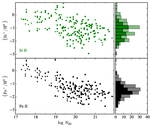
Figure 14.— Comparison of the $\{{\rm Si}^{+}/{\rm H}^{0}\}$ and $\{{\rm Fe}^{+}/{\rm H}^{0}\}$ measurements for the LLSs and DLAs. The latter are drawn from the abundance compilation of Rafelski et al. (2012). For both ions, the DLAs show a continuous extension of the measurements observed in the LLSs. The right hand panels compare the distributions of the DLAs (darker) against those for the SLLSs (lighter), and emphasize the commonality between the two datasets. In each case, we have treated upper and lower limit estimates as values.

6.4. Comparisons

We have restricted the HD-LLS Sample to systems with $N_{\rm HI}<10^{20.3}\,{\rm cm^{-2}}$ to exclude the DLAs. This was partly motivated by the expectation that the majority of LLSs are predominantly ionized and therefore physically distinct from the neutral gas comprising DLAs. It was also motivated by the desire to examine this optically thick gas separately from the decades of research on the DLAs. Nonetheless, the $N_{\rm HI}=10^{20.3}\,{\rm cm^{-2}}$ criterion is primarily an observationally defined boundary and one may gain insight into the nature of the LLSs through a combined comparison. Such analysis has been performed previously for the SLLS by peroux03; Som et al. (2013).

We consider two such comparisons here. Figure 14 presents the $\{{\rm Si}^{+}/{\rm H}^{0}\}$ and $\{{\rm Fe}^{+}/{\rm H}^{0}\}$ measurements for the HD-LLS Sample together with measurements from the sample of DLAs of Rafelski et al. (2012). For both datasets, we have restricted to $z_{\rm abs}=[1.6,3.3]$ to minimize trends related to redshift evolution. To zeroth order, the DLA measurements extend in a roughly continuous manner from the measurements of the LLSs. Indeed, comparing the samples of DLA measurements with the SLLSs (taking limits at their values), one observes overlapping distributions with similar median values. The only notable distinction, perhaps, is the small set of LLSs with $N_{\rm HI}\approx 10^{19}\,{\rm cm^{-2}}$ and high $\{{\rm X}^{i}/{\rm H}^{0}\}$ values (exceeding 0 dex for Si⁺). This suggests a higher incidence of highly enriched gas in the LLS, although we caution it could be partly an effect of ionization. The dispersion in the measurements is also larger for the LLSs, and is likely higher than suggested by the Figure given the preponderance of upper/lower limits for the LLS/DLA.

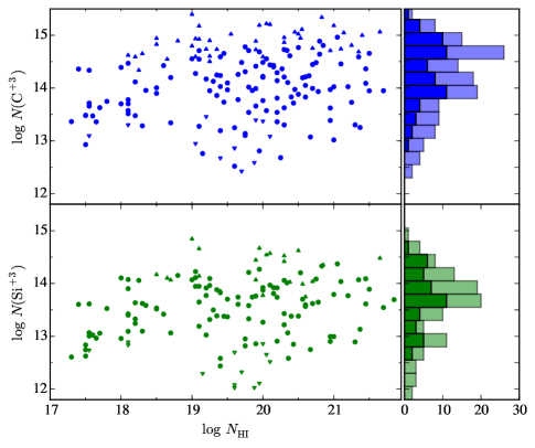
Figure 15.— Comparison of the high-ion column densities measured for the LLS and a representative set of DLAs (drawn from Rafelski et al., 2012; Neeleman et al., 2013). Similar to the low-ion abundances, the measurements show a continuous transition from the LLS regime to higher $N_{\rm HI}$ values. As such, there is substantial overlap in the distribution of measurements and limits (right-hand panels compare the values for DLAs [darker] and SLLSs [lighter]). One notable and surprising difference is that the SLLSs show a higher incidence of low columns of C⁺³ and Si⁺³. Despite tracing predominantly neutral gas, the DLAs also mark a reservoir of highly ionized gas that frequently exceeds the medium encompassing the LLSs.

Turning to the higher ionization states, Figure 15 presents the C⁺³ and Si⁺³ column densities from the LLSs and DLAs. Once again, the DLA distribution extends in a nearly continuous manner from the upper end of the LLS data and the column density distributions for the SLLSs and DLAs are similar. Together, Figures 14 and 15 lend support to scenarios that envision LLSs as the outer layers of gas surrounding DLAs, i.e. these systems frequently sample the same structures. Such physical associations may be examined by studying DLAs and LLSs along pairs of quasar sightlines, an active area of research (Ellison et al., 2007; Fumagalli et al., 2014; Rubin et al., 2014).

Examining the high-ion comparison further, there is at least one import distinction: the LLSs and especially the SLLSs show a much higher incidence of low ${N({\rm C^{+3}})}$ and ${N({\rm Si^{+3}})}$ values. This is unexpected given that (i) the LLSs trace highly ionized gas; (ii) the DLAs trace predominantly neutral gas that is physically distinct from the high-ions (Wolfe & Prochaska, 2000; Prochaska et al., 2008a). The results presented here indicate that the gas layers giving rise to DLAs are embedded in a reservoir of highly ionized gas that frequently exceeds the typical surface density in LLSs. This follows previous work which has inferred high quantities of both neutral and ionized gas for the DLAs (Fox et al., 2007; Lehner et al., 2014). It further suggests that high-ions more closely trace higher density regions in the universe and/or may reflect a difference in the masses of the dark matter halos hosting LLSs and DLAs.

Lastly, we have compared our measurements against the small set of literature values for SLLSs at $z>2$ (Dessauges-Zavadsky et al., 2003; Som et al., 2013). The low-ion column densities are typically larger in those publications, consistent with the higher $N_{\rm HI}$ values of the SLLSs that were sampled.

7. Summary

We have constructed a sample of 157 LLSs at $z\sim 2-4$ observed at high-dispersion with spectrometers on the Keck and Magellan telescopes which constitute the HD-LLS Sample. In this manuscript, we present the complete sample and present column density measurements of H I and associated metal absorption. For the latter, analysis was restricted to transitions redward of the Ly$\alpha$ forest and has focused on commonly detected species. These measurements and the associated spectra are made available online with this publication. This constitutes, by roughly an order of magnitude, the largest high redshift sample of LLS analyzed in this manner.

We have explored empirical trends in the column density measurements and report statistically significant ($>99.99\%$) correlations between the low-ion (e.g. Si⁺, C⁺) columns and $N_{\rm HI}$. High-ion species (Si⁺³, C⁺³) are detected in nearly all LLSs and their column densities also correlated with $N_{\rm HI}$. Examining ionic ratios sensitive to the ionization state (e.g. C⁺³/C⁺, Si⁺³/Si⁺), we conclude that the LLSs are predominantly ionized with more highly ionized gas in lower $N_{\rm HI}$ systems.

Ratios of low-ion column densities to $N_{\rm HI}$ indicate a wide spread in metal-enrichment within the LLSs, likely spanning four orders of magnitude. Only a small subset ($\lesssim 5\%$) of the HD-LLS Sample have no positive detections of associated metals, consistent with primordial abundances. None of the LLSs with $N_{\rm HI}\geq 10^{19.2}\,{\rm cm^{-2}}$ are ‘metal-free’. We conclude that a very high percentage of high-density gas at $z\sim 3$ was previously enriched to $\gtrsim 1/1000$ solar abundance. The HD-LLS Sample also exhibits a small subset ($\sim 10\%$) of LLSs that have solar or super-solar enrichment. These likely represent the most enriched gas reservoirs in the high redshift universe.

Lastly, we have examined several ionic ratios that are sensitive to the nucleosynthetic enrichment history of the gas. The preponderance of elevated Si⁺/Fe⁺ and O⁰/Fe⁺ measurements suggest the LLSs have an $\alpha$-enhancement characteristic of Type II nucleosynthesis. In contrast, the Si⁺/C⁺ and Al⁺/C⁺ ratios are consistent with solar relative abundances.

Future manuscripts on the HD-LLS Sample will: (i) study the metallicity distribution of the LLSs accounting for ionization effects and will estimate the contribution of optically thick gas to the cosmic metal budget; (ii) examine the kinematic characteristics to constrain the physical origin of the gas; (iii) offer constraints on the $N_{\rm HI}$ frequency distribution for optically thick gas.

Table 6IONIC COLUMN DENSITIES

Quasar	RA	DEC	$z_{\rm abs}$	$N_{\rm HI}$	$\lambda$	$v_{\rm lim}$	flg	$N_{\lambda}$	$\sigma(N)$	Ion	flg	$N_{\rm ion}$	$\sigma(N)$
	(J2000)	(J2000)			(Å)	(km/s)
Q0001-2340	00:03:45	-23:23:46.5	2.18710	19.65	1334.5323	$-423,64$	2	14.45	99.99	6,2	2	14.45	99.99
					1335.7077	$-205,64$	4	13.10	99.99
					1548.1950	$-423,64$	0	14.26	0.01	6,4	1	14.26	0.05
					1550.7700	$-394,64$	0	14.25	0.02
					1302.1685	$-213,64$	0	14.16	0.04	8,1	1	14.16	0.05
					2852.9642	$-213,64$	4	11.72	99.99	12,1	3	11.72	99.99
					2796.3520	$-413,64$	2	13.43	99.99	12,2	1	13.64	0.05
					2803.5310	$-404,64$	0	13.65	0.02
					1670.7874	$-405,64$	2	13.00	99.99	13,2	2	13.00	99.99
					1854.7164	$-213,64$	4	12.40	99.99	13,3	3	12.40	99.99
					1862.7895	$-213,64$	4	12.69	99.99
					1260.4221	$-399,64$	2	13.81	99.99	14,2	1	13.75	0.05
					1304.3702	$-423,64$	0	13.55	0.09
					1526.7066	$-399,64$	0	13.83	0.03
					1808.0130	$-213,64$	4	14.86	99.99
					1393.7550	$-411,64$	0	13.78	0.01	14,4	1	13.74	0.05
					1402.7700	$-421,64$	0	13.64	0.02
					1250.5840	$-79,64$	0	14.19	0.13	16,2	1	14.19	0.13
					1608.4511	$-213,64$	4	13.49	99.99	26,2	1	13.11	0.05
					2344.2140	$-213,64$	0	13.22	0.07
					2374.4612	$-213,64$	4	13.46	99.99
					2382.7650	$-213,64$	0	13.01	0.04
					2586.6500	$-213,64$	4	13.15	99.99
					2600.1729	$-328,64$	0	13.25	0.04
					1317.2170	$-213,64$	4	13.41	99.99	28,2	3	13.40	99.99
					1370.1310	$-213,64$	4	13.40	99.99
					1454.8420	$-213,64$	4	13.56	99.99
					1741.5531	$-213,64$	4	13.60	99.99
					1751.9157	$-213,64$	4	13.83	99.99
					2026.1360	$-213,64$	4	12.38	99.99	30,2	3	12.38	99.99
PX0034+16	00:34:54.8	+16:39:20	3.75397	20.05	1548.1950	$-242,65$	0	13.85	0.02	6,4	1	13.85	0.05
					1550.7700	$-118,189$	2	13.68	99.99
					1670.7874	$-187,189$	0	12.52	0.04	13,2	1	12.52	0.05
					1854.7164	$-115,120$	4	12.24	99.99	13,3	3	12.24	99.99
					1862.7895	$-89,129$	4	12.57	99.99
					1526.7066	$-54,122$	2	14.06	99.99	14,2	2	14.06	99.99
					1808.0130	$-133,138$	4	14.73	99.99
					1393.7550	$-160,133$	0	13.30	0.02	14,4	1	13.30	0.05
					1741.5531	$-187,189$	4	14.29	99.99	28,2	3	13.72	99.99
					1751.9157	$-86,189$	4	13.72	99.99
					2026.1360	$-187,189$	4	13.16	99.99	30,2	3	13.16	99.99

Note. — Columns are as follows: (1) Quasar name; (2,3) RA/DEC; (4) Absorption redshift of LLS; (5) HI column Density; (6) Rest wavelength of transition; (7) Velocity limits (min/max) for integration relative to $z_{\rm abs}$; (8) Flag on individual measurement: [0,1=standard measurement; 2,3=Lower limit; 4,5=Upper limit]; (9) $\log_{10}$ column density; (10) Standard deviation on $\log_{10}N$. Limits are given a value of 99.99; (11) Ion [atomic number, ionization state]; (12) Flag for the ionic column density [1=standard measurement; 2=Lower limit; 3=Upper limit]; (13) $\log_{10}$ column density for the ion; (14) Standard deviation on $\log_{10}N_{\rm ion}$. Limits are given a value of 99.99;

Note. — [The complete version of this table is in the electronic edition of the Journal. The printed edition contains only a sample.]

Fig. Set16. Velocity Plots for the Lyman Limit Systems

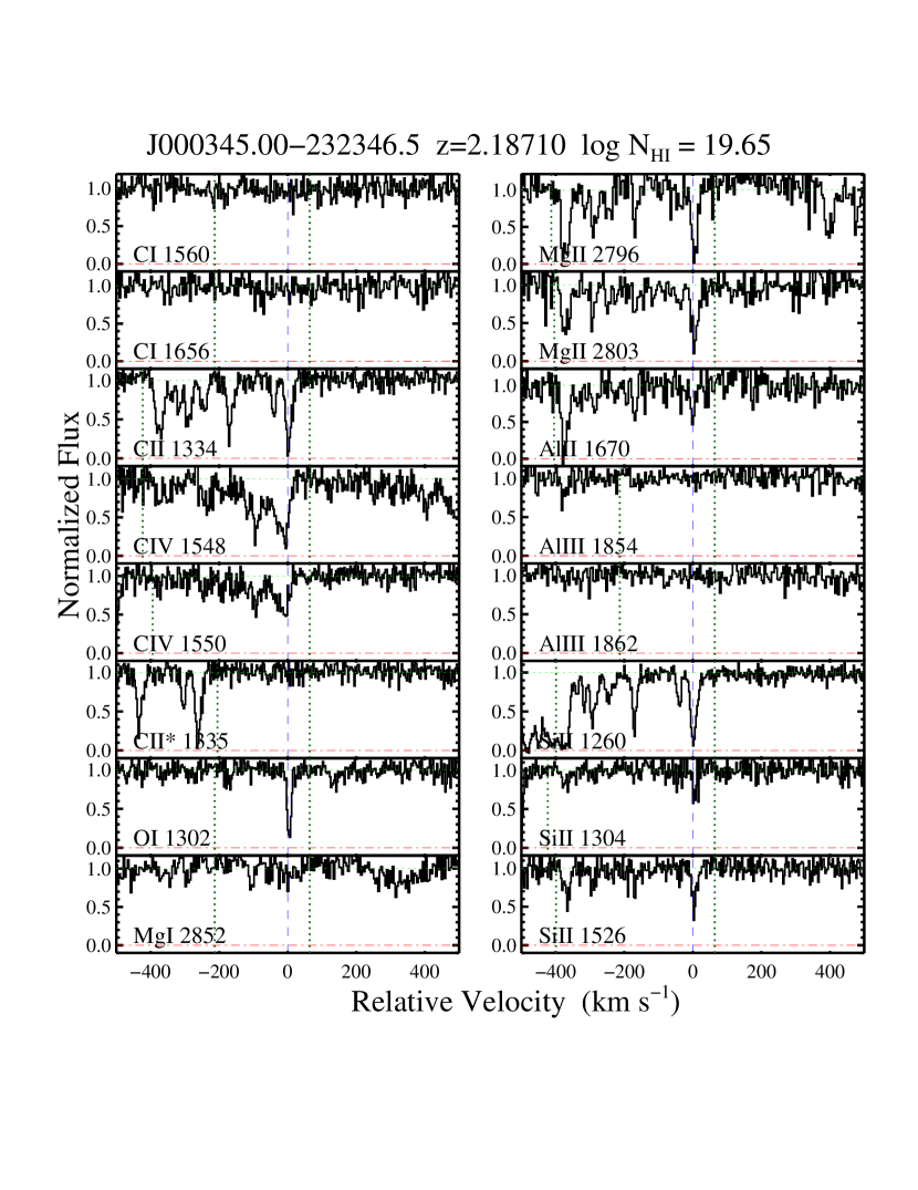
Figure 16.— Velocity plots for the HD-LLS Sample

References

- Aguirre et al. (2001) Aguirre, A., Hernquist, L., Schaye, J., Weinberg, D. H., Katz, N., & Gardner, J. 2001, ApJ, 560, 599
- Aguirre et al. (2004) Aguirre, A., Schaye, J., Kim, T.-S., Theuns, T., Rauch, M., & Sargent, W. L. W. 2004, ApJ, 602, 38
- Asplund et al. (2009) Asplund, M., Grevesse, N., Sauval, A. J., & Scott, P. 2009, ArXiv e-prints
- Berg et al. (2014) Berg, T. A. M., Neeleman, M., Prochaska, J. X., Ellison, S. L., & Wolfe, A. M. 2014, ArXiv e-prints
- Bernstein et al. (2003) Bernstein, R., Shectman, S. A., Gunnels, S. M., Mochnacki, S., & Athey, A. E. 2003, in Instrument Design and Performance for Optical/Infrared Ground-based Telescopes. Edited by Iye, Masanori; Moorwood, Alan F. M. Proceedings of the SPIE, Volume 4841, pp. 1694-1704 (2003)., 1694–1704
- Bochanski et al. (2009) Bochanski, J. J., et al. 2009, PASP, 121, 1409
- Bouché et al. (2006) Bouché, N., Lehnert, M. D., & Péroux, C. 2006, MNRAS, 367, L16
- Burles & Tytler (1998) Burles, S., & Tytler, D. 1998, ApJ, 499, 699
- Chen et al. (2010) Chen, H., Helsby, J. E., Gauthier, J., Shectman, S. A., Thompson, I. B., & Tinker, J. L. 2010, ApJ, 714, 1521
- Dekel et al. (2009) Dekel, A., et al. 2009, Nature, 457, 451
- Dessauges-Zavadsky et al. (2003) Dessauges-Zavadsky, M., Péroux, C., Kim, T.-S., D’Odorico, S., & McMahon, R. G. 2003, MNRAS, 345, 447
- Ellison et al. (2007) Ellison, S. L., Hennawi, J. F., Martin, C. L., & Sommer-Larsen, J. 2007, MNRAS, 378, 801
- Faucher-Giguere et al. (2014) Faucher-Giguere, C.-A., Hopkins, P. F., Keres, D., Muratov, A. L., Quataert, E., & Murray, N. 2014, ArXiv e-prints
- Faucher-Giguère & Kereš (2011) Faucher-Giguère, C.-A., & Kereš, D. 2011, MNRAS, 412, L118
- Faucher-Giguère et al. (2008) Faucher-Giguère, C.-A., Prochaska, J. X., Lidz, A., Hernquist, L., & Zaldarriaga, M. 2008, ApJ, 681, 831
- Fox et al. (2007) Fox, A. J., Petitjean, P., Ledoux, C., & Srianand, R. 2007, A&A, 465, 171
- Fumagalli et al. (2014) Fumagalli, M., Hennawi, J. F., Prochaska, J. X., Kasen, D., Dekel, A., Ceverino, D., & Primack, J. 2014, ApJ, 780, 74
- Fumagalli et al. (2011a) Fumagalli, M., O’Meara, J. M., & Prochaska, J. X. 2011a, Science, 334, 1245
- Fumagalli et al. (2013) Fumagalli, M., O’Meara, J. M., Prochaska, J. X., & Worseck, G. 2013, ApJ, 775, 78
- Fumagalli et al. (2011b) Fumagalli, M., Prochaska, J. X., Kasen, D., Dekel, A., Ceverino, D., & Primack, J. R. 2011b, MNRAS, 418, 1796
- Hennawi & Prochaska (2007) Hennawi, J. F., & Prochaska, J. X. 2007, ApJ, 655, 735
- Jenkins (2009) Jenkins, E. B. 2009, ApJ, 700, 1299
- Kereš et al. (2005) Kereš, D., Katz, N., Weinberg, D. H., & Davé, R. 2005, MNRAS, 363, 2
- Lehner et al. (2013) Lehner, N., et al. 2013, ApJ, 770, 138
- Lehner et al. (2014) Lehner, N., O’Meara, J. M., Fox, A. J., Howk, J. C., Prochaska, J. X., Burns, V., & Armstrong, A. A. 2014, ApJ, 788, 119
- Marshall et al. (2008) Marshall, J. L., et al. 2008, in Society of Photo-Optical Instrumentation Engineers (SPIE) Conference Series, Vol. 7014, Society of Photo-Optical Instrumentation Engineers (SPIE) Conference Series
- McWilliam (1997) McWilliam, A. 1997, ARA&A, 35, 503
- Neeleman et al. (2013) Neeleman, M., Wolfe, A. M., Prochaska, J. X., & Rafelski, M. 2013, ApJ, 769, 54
- O’Meara et al. (2006) O’Meara, J. M., Burles, S., Prochaska, J. X., Prochter, G. E., Bernstein, R. A., & Burgess, K. M. 2006, ApJ, 649, L61
- O’Meara et al. (2007) O’Meara, J. M., Prochaska, J. X., Burles, S., Prochter, G., Bernstein, R. A., & Burgess, K. M. 2007, ApJ, 656, 666
- O’Meara et al. (2013) O’Meara, J. M., Prochaska, J. X., Worseck, G., Chen, H.-W., & Madau, P. 2013, ApJ, 765, 137
- Peeples et al. (2014) Peeples, M. S., Werk, J. K., Tumlinson, J., Oppenheimer, B. D., Prochaska, J. X., Katz, N., & Weinberg, D. H. 2014, ApJ, 786, 54
- Penprase et al. (2010) Penprase, B. E., Prochaska, J. X., Sargent, W. L. W., Toro-Martinez, I., & Beeler, D. J. 2010, ApJ, 721, 1
- Péroux et al. (2005) Péroux, C., Dessauges-Zavadsky, M., D’Odorico, S., Sun Kim, T., & McMahon, R. G. 2005, MNRAS, 363, 479
- Prochaska (1999) Prochaska, J. X. 1999, ApJ, 511, L71
- Prochaska et al. (2008a) Prochaska, J. X., Chen, H.-W., Wolfe, A. M., Dessauges-Zavadsky, M., & Bloom, J. S. 2008a, ApJ, 672, 59
- Prochaska et al. (2003a) Prochaska, J. X., Gawiser, E., Wolfe, A. M., Castro, S., & Djorgovski, S. G. 2003a, ApJ, 595, L9
- Prochaska et al. (2003b) Prochaska, J. X., Gawiser, E., Wolfe, A. M., Cooke, J., & Gelino, D. 2003b, ApJS, 147, 227
- Prochaska & Hennawi (2009) Prochaska, J. X., & Hennawi, J. F. 2009, ApJ, 690, 1558
- Prochaska et al. (2008b) Prochaska, J. X., Hennawi, J. F., & Herbert-Fort, S. 2008b, ApJ, 675, 1002
- Prochaska et al. (2013) Prochaska, J. X., et al. 2013, ApJ, 776, 136
- Prochaska et al. (2014a) Prochaska, J. X., Lau, M. W., & Hennawi, J. F. 2014a, ApJ, 796, 140
- Prochaska et al. (2014b) Prochaska, J. X., Madau, P., O’Meara, J. M., & Fumagalli, M. 2014b, MNRAS, 438, 476
- Prochaska et al. (2006) Prochaska, J. X., O’Meara, J. M., Herbert-Fort, S., Burles, S., Prochter, G. E., & Bernstein, R. A. 2006, ApJ, 648, L97
- Prochaska et al. (2010) Prochaska, J. X., O’Meara, J. M., & Worseck, G. 2010, ApJ, 718, 392
- Prochaska & Wolfe (1997) Prochaska, J. X., & Wolfe, A. M. 1997, ApJ, 487, 73
- Prochaska et al. (2007) Prochaska, J. X., Wolfe, A. M., Howk, J. C., Gawiser, E., Burles, S. M., & Cooke, J. 2007, ApJS, 171, 29
- Prochaska et al. (2001) Prochaska, J. X., et al. 2001, ApJS, 137, 21
- Prochaska et al. (2009) Prochaska, J. X., Worseck, G., & O’Meara, J. M. 2009, ApJ, 705, L113
- Prochter et al. (2010) Prochter, G. E., Prochaska, J. X., O’Meara, J. M., Burles, S., & Bernstein, R. A. 2010, ApJ, 708, 1221
- Rafelski et al. (2012) Rafelski, M., Wolfe, A. M., Prochaska, J. X., Neeleman, M., & Mendez, A. J. 2012, ApJ, 755, 89
- Ribaudo et al. (2011) Ribaudo, J., Lehner, N., & Howk, J. C. 2011, ApJ, 736, 42
- Rubin et al. (2014) Rubin, K. H. R., Hennawi, J. F., Prochaska, J. X., Simcoe, R. A., Myers, A., & Wingyee Lau, M. 2014, ArXiv e-prints
- Rudie et al. (2012) Rudie, G. C., et al. 2012, ApJ, 750, 67
- Sargent et al. (1989) Sargent, W. L. W., Steidel, C. C., & Boksenberg, A. 1989, ApJS, 69, 703
- Savage & Sembach (1991) Savage, B. D., & Sembach, K. R. 1991, ApJ, 379, 245
- Schaye et al. (2003) Schaye, J., Aguirre, A., Kim, T.-S., Theuns, T., Rauch, M., & Sargent, W. L. W. 2003, ApJ, 596, 768
- Sheinis et al. (2002) Sheinis, A. I., Bolte, M., Epps, H. W., Kibrick, R. I., Miller, J. S., Radovan, M. V., Bigelow, B. C., & Sutin, B. M. 2002, PASP, 114, 851
- Simcoe (2011) Simcoe, R. A. 2011, ApJ, 738, 159
- Sofia & Jenkins (1998) Sofia, U. J., & Jenkins, E. B. 1998, ApJ, 499, 951
- Som et al. (2013) Som, D., Kulkarni, V. P., Meiring, J., York, D. G., Péroux, C., Khare, P., & Lauroesch, J. T. 2013, MNRAS, 435, 1469
- Songaila & Cowie (2010) Songaila, A., & Cowie, L. L. 2010, ApJ, 721, 1448
- Steidel (1990) Steidel, C. C. 1990, ApJS, 74, 37
- Steidel et al. (2010) Steidel, C. C., Erb, D. K., Shapley, A. E., Pettini, M., Reddy, N., Bogosavljević, M., Rudie, G. C., & Rakic, O. 2010, ApJ, 717, 289
- Storrie-Lombardi et al. (1994) Storrie-Lombardi, L. J., McMahon, R. G., Irwin, M. J., & Hazard, C. 1994, ApJ, 427, L13
- Tinsley (1979) Tinsley, B. M. 1979, ApJ, 229, 1046
- Tytler (1982) Tytler, D. 1982, Nature, 298, 427
- Vogt et al. (1994) Vogt, S. S., et al. 1994, in Proc. SPIE Instrumentation in Astronomy VIII, David L. Crawford; Eric R. Craine; Eds., Volume 2198, p. 362, 362–+
- Werk et al. (2013) Werk, J. K., Prochaska, J. X., Thom, C., Tumlinson, J., Tripp, T. M., O’Meara, J. M., & Peeples, M. S. 2013, ApJS, 204, 17
- Wolfe & Prochaska (2000) Wolfe, A. M., & Prochaska, J. X. 2000, ApJ, 545, 591
- Worseck et al. (2014) Worseck, G., et al. 2014, MNRAS, 445, 1745
- Zafar et al. (2013) Zafar, T., Popping, A., & Péroux, C. 2013, A&A, 556, A140