Dropout as data augmentation

Abstract

Dropout is typically interpreted as bagging a large number of models sharing parameters. We show that using dropout in a network can also be interpreted as a kind of data augmentation in the input space without domain knowledge. We present an approach to projecting the dropout noise within a network back into the input space, thereby generating augmented versions of the training data, and we show that training a deterministic network on the augmented samples yields similar results. Finally, we propose a new dropout noise scheme based on our observations and show that it improves dropout results without adding significant computational cost.

1 Introduction

Noise is normally seen as intrinsically undesirable. The word itself bears a very negative connotation. It is not surprising then that many early mathematical models in neuroscience aimed to factor out noise by any means. A few decades ago, the use of stochastic resonance (Wiesenfeld et al., 1995) in neuro-scientific models initiated a new interest in neurosience regarding random fluctuations and the role they play in the brain. Theories about neuronal noise are now flourishing and previous deterministic models are improved by the incorporation of noise (Yarom & Hounsgaard, 2011).

Biological brains have always been a strong inspiration when it comes to developing learning algorithms. Considering the amount of noise which takes place in the brain during learning, one can wonder if this has any beneficial effect. Many techniques in machine learning have made use of noise to improve performance recently, namely, Denoising Autoencoders (Vincent et al., 2008), dropout (Hinton et al., 2012) and its relative, DropConnect (Wan et al., 2013). Those successful approaches suggest that neuronal noise plays a fundamental role in the process of learning and should be studied more thoroughly.

Using dropout can be viewed as training a huge number of neural networks with shared parameters and applying bagging at test time for better generalization (Baldi & Sadowski, 2013). Binary noise can also be viewed as preventing neurons from co-adapting, which improves the generalization of the model even more. In this paper, we propose an alternative view and suggest noise schemes like dropout are implicitly incorporating a form of sophisticated data augmentation. In Section 3, we formulate a method to generate data which replicates dropout noise within a deterministic network, and demonstrate in Section 5 that there is no significant loss of accuracy.

Finally, capitalizing on the idea of data augmentation, we present in section 4 an extension of dropout which uses random noise levels to improve the variety of samples. This simple extension improves classification performance across different network architectures, yielding competitive results on the MNIST permutation invariant classification task.

2 Dropout

The main goal when using dropout is to regularize the neural network we are training. The technique consists of dropping neurons randomly with some probability $p$. Those random modifications of the network’s stucture are believed to avoid co-adaptation of neurons by making it impossible for two subsequent neurons to rely solely on each other (Srivastava et al., 2014). The most accepted interpretation of dropout is that is implicitely bagging at test time a large number of neural networks which share parameters.

Assume $h(x)$ is a linear projection of a $d_{i}$-dimensional input $x$ into a $d_{h}$-dimensional space:

$$h(x)=xW+b$$ (1)

Given $a(h)$ and $\tilde{a}(h)$, an activation function and its noisy version where $M\sim\mathcal{B}(p_{h})$ and $\mbox{rect}(h)$ is a rectifier

$$a(h) =\mbox{rect}(h)$$ (2)

$$\tilde{a}(h) =M\odot\mbox{rect}\left(h\right)$$ (3)

Eq. 3 denotes the activation with dropout during training and eq. 2 the equation of the activation at test time. Srivastava et al. (2014) suggest to scale the activations $a(h)$ with $p$ at test time to get an approximate average of the unit activation.

3 From a data augmentation perspective

In many previous works it has been shown that augmenting data by using domain specific transformations helps in learning better models (LeCun et al., 1998; Simard et al., 2003; Krizhevsky et al., 2012; Ciresan et al., 2012). In this work, we analyze dropout in the context of data augmentation. Considering the task of classification, given a set of training samples, the objective would be to learn a mapping function which maps every input to its corresponding output label. To generalize, the mapping function needs to be able to correctly map not just the training samples but also any other samples drawn from the data distribution. This means that it must not only map input space sub-regions represented by training samples, but all high-probability sub-regions of the natural distribution.

One way to learn such a mapping function is by augmenting the training data such that it covers a larger portion of the natural distribution. Domain-based data augmentation helps to artificially boost training data coverage which makes it possible to train a better mapping function. We hypothesize that noise based regularization techniques result in a similar effect of increasing training data coverage at every hidden layer and this work presents multiple experimental observations to support our hypothesis.

3.1 Projecting noise back into the input space

We assume that for a given $\tilde{a}(h)$, there exist an $x^{*}$, such that

$$(a\circ h)(x^{*})=\mbox{rect}(h(x^{*}))\approx\vec{m}\odot\mbox{rect}\left(h(x)\right)=(\tilde{a}\circ h)(x)$$ (4)

Similarly to adversarial examples from Goodfellow et al. (2014b), an $x^{*}$ can be found by minimizing the squared error $L$ using stochastic gradient descent

$$L\left(x,x^{*})\right)=\left|(a\circ h)(x^{*})-(\tilde{a}\circ h)(x)\right|^{2}$$ (5)

Equation 5 can be generalized to a network with $n$ hidden layers. To lighten notation we first define

$$\tilde{f}^{(i)}(x) =\left(\tilde{a}^{(i)}\circ h^{(i)}\circ\dots\circ\tilde{a}^{(1)}\circ h^{(1)}\right)(x)$$ (6)

$$f^{(i)}(x^{*}) =\left(a^{(i)}\circ h^{(i)}\circ\dots\circ a^{(1)}\circ h^{(1)}\right)(x^{*})$$ (7)

We can now compute the back projection corresponding to all hidden layer activations at once, which results in minizing the loss $L$

$$L\left(x,x^{(1)^{*}},\dots,x^{(n)^{*}}\right)=\sum_{i=1}^{n}\lambda_{i}\left|f^{(i)}\left(x^{(i)^{*}}\right)-\tilde{f}^{(i)}(x)\right|^{2}$$ (8)

We can show by contradiction that one is unlikely to find a single ${x^{*}=x^{(1)^{*}}=x^{(2)^{*}}=\dots=x^{(n)^{*}}}$ that significantly reduces $L$. The proof is detailed in appendix subsection 8.1. Fortunately, it is easy to find a different $x^{*}$ for each hidden layer, by providing multiple inputs $(x,x^{(1)^{*}},x^{(2)^{*}},\dots,x^{(n)^{*}})$, where $n$ is the number of hidden layers. As each $x^{(i)^{*}}$ is the back projection of a transformation in the representation space defined by the $i$-th hidden layer, it suggests viewing dropout as a sophisticated data augmentation procedure that samples data around training examples with respect to different level of representations. This raises the question whether we can train the network deterministically on the $x^{(i)^{*}}$ rather than using dropout. The answer is not trivial, because

1. When using $(x,x^{(1)^{*}},x^{(2)^{*}},\dots,x^{(n)^{*}})$ as inputs, dropout is not effectively applied to every layer at the same time. The local stochasticity preventing co-adaptation is then present at a specific layer only once for every $x^{(i)^{*}}$. This could be not aggressive enough to avoid co-adaptation.

2. The gradients of the linear projections will differ greatly. In the case of dropout, $\frac{\partial{h}}{\partial{W^{(i)}}}$ is always equal to its input transformation, i.e. $\tilde{f}^{(i-1)}(x)$, whereas the deterministic version of the training will update $W^{(i)}$ according to $\left(f^{(i-1)}(x^{(1)^{*}}),\dots,f^{(i-1)}(x^{(n)^{*}})\right)$.

Although we proved a single $x^{*}$ minimising 8 is difficult to find for a large network, we show experimentally in section 5 that it is possible to do so within reasonable approximation for a relatively small two hidden layer network. We further show that dropout can be replicated by projecting the noise back on the input space without a significant loss of accuracy.

4 Improving the set of augmentations

When dealing with domain-based transformations, we intuitively look for the richest set of transformations. In computer vision for instance, translations, rotations, scalings, shearings and elastic transformations are often combined. Looking at dropout from a data augmentation perspective, this intuition raises the following question: given that noise scheme used is implicitely applying some transformations in the input space, which one would produce the richest set of transformations?

With noise schemes like dropout, there are two important components which influence the transformations; The probability distribution of $\vec{m}$ and the features of the neural network used to encode $h(x)$. Modifying the probability distribution is the most straighforward way to improve the set of transformations and will be the main focus of this paper. However, features of the neural network play a key role in the transformations and we will outline some possible avenues in the conclusion section.

4.1 Random noise levels

While using dropout, the proportion of neurons dropped is very close to probability $p$. It follows naturally from Binomial distribution’s expectation. The transformations induced are as different as the values $M$ can take. Despite this, their magnitude is as constant as the proportion of neurons dropped. That means, every transformations displaces the sample to a relatively constant distance but in random directions in a high dimensional space.

A simple way to vary the transformation magnitude randomly is to replace $p$ by a random variable. Let $\rho_{h}\sim\mathcal{U}(0,p_{h})$ and $M_{hij}\sim\mathcal{B}(\rho_{h})$ where $h$ defines the layer, $i$ the sample, and $j$ the layer’s neuron. It is important to use the same $\rho$ for all neurons of a layer, otherwise we would have $M_{hij}\sim\mathcal{B}(\frac{p_{h}}{2})$.

To compensate for the change of level of activations during test, a scaling is normally applied. One could also simply apply the inverse scaling during training, turning equation 3 into

$$\tilde{a}(h)=\frac{1}{1-p}M\odot\mbox{rect}\left(h\right)$$ (9)

To adapt the equation to random dropout level, we simply need to replace $p$ with $\rho$

$$\tilde{a}(h)=\frac{1}{1-\rho}M\odot\mbox{rect}\left(h\right)$$ (10)

No scaling needs to be done during test anymore.

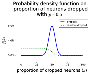
Figure 1: The density function on proportion of neurons dropped is very peaked around $p$ for dropout. This results in a low variance of the transformations magnitude induced by dropout. Random dropout on the other hand has a constant density function under $pN$, $N$ being the number of neurons, because $\rho\sim\mathcal{U}(0,p)$. It is thus more likely to see transformations closer to identity while it is very unlikely for standard dropout. This is intuitively desirable, as much as varying translation distances is preferable over constant large distances.

Figure 1 shows the differences between density function on proportion of neurons dropped for dropout and random dropout. Transformations induced by random dropout are clearly more diverse than those induced by dropout.

5 Experiments

5.1 Visualizations of noise projected back into the input space

Visualizing the noise projected back into the input space helps to understand what kind of transformations are induced by dropout. Unsupervised models learn more general features than supervised fully connected neural networks and produce thus more visually appealing transformations. For this reason, we trained autoencoders with dropout on the hidden layer to generate samples of transformations.

The autoencoder is very similar to denoising autoencoders, the only difference is that a Bernoulli mask is applied to the hidden activations rather than to the input. There is thus no noise applied to the input explicitly. Models are trained for 300 epochs, with mini-batch size of 100, $p$ = 0.4, a learning rate of 0.001 on MNIST, 0.0001 on CIFAR-10 and a momentum of 0.7 on MNIST, 0.5 on CIFAR-10. For CIFAR-10, we do preprocessing with PCA dimensionality reduction and retain 781 features.

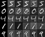
(a) MNIST

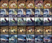
(b) CIFAR

Figure 5: Visualization of noisy samples from random dropout on MNIST and CIFAR-10. The first column represent original samples from MNIST and CIFAR-10 datasets. Each row contains samples from the same original sample. Every other column represents noisy samples produced by back-projecting the noise into the input space. Each one is induced by a different noise mask and a different noise level, i.e. a different value of $\rho$ and $M$. The transformations from figure 5 and this one are clearly different. Random dropout applies transformations with different strenghs, i.e., the transformed input can be very close to very far from the original input while standard dropout always applies transformations with the same strengh.

Once the model is trained, we use gradient descent to compute $x^{*}$ as described in 3.1. We iterate for 10 epochs with a learning rate of 100 for both MNIST and CIFAR-10. Figure 5 shows well how close $x^{*}$ are from the natural input space and we clearly see that the classes are still distinguishable.

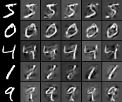
(a) MNIST

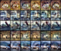
(b) CIFAR

Figure 2: Visualization of noisy samples on MNIST and CIFAR-10. The first column represent original samples from MNIST and CIFAR-10 datasets. Each row contains samples from the same original sample. Every other column represents noisy samples produced by back-projecting the noise into the input space. Each one is induced by a different noise mask, i.e. a different value of $M$.

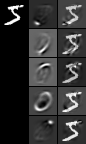
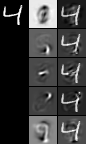
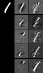
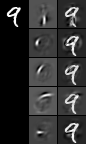
Figure 3: Visualization of the influence of the features on the transformations induced by dropout on MNIST. First column represent original samples from MNIST dataset. Second column represents the five most active features on each given original sample. Last column represents noisy samples produced by back-projecting the noise into the input space while keeping the selected feature shut off to 0. We can see that the features are not simply removed from the input, but rather destroyed in such a way that other features highly dependant on the same subregion still have the same activation level.

To help understand how each feature influences the transformation, we isolate five most active features for a given input and shut them off, each separately. For each feature shut off, we compute $x^{*}$ using gradient descent. Figure 3 shows the results found for MNIST. One could think the features dropped by the noise are simply removed from the input. It turns out removing the feature would affect the activation of other neurons. Because of this, features are rather destroyed in the input in such a way that other features highly dependant on the same subregion still have the same activation level.

5.2 Equivalence of dropout and noisy samples

We ran a series of experiments with fully connected feed forward neural networks on the MNIST and CIFAR-10 datasets to study the effect of replacing dropout by corresponding noisy inputs. Each network consists of two hidden layers with rectified linear units followed by a softmax layer. We experimented with four different architectures each one with a different number of units in the hidden layers: 2500-2500, 2500-1250, 1500-1500 and 1500-750.

The MNIST dataset consists of $60000$ training samples and $10000$ test samples. We split the training set into a set of $50000$ samples for training and $10000$ for validation. Each network is trained for $501$ epochs and the best model based on validation error is selected. Later the best model is further trained on the complete training set of $60000$ samples (training + validation split) for another $150$ epochs. The mean error percentage for the last $75$ epochs is used for comparison.

We also ran experiments on the CIFAR-10 permutation invariant task using the same network architectures described above. The dataset consists of $50000$ training samples and $10000$ test samples. We use PCA based dimensionality reduction without whitening as preprocessing scheme, retaining 781 features. We used the same approach as in the MNIST experiments to train the networks and for reporting the performances.

At each epoch, an $x^{*}$ is generated for each training sample. It proved to be possible to find good $x^{*}$ approximations for the entire network at once for a 2-hidden layer network. Thus, we trained on $x$ and $x^{*}$ solely rather than $x$, $x^{(1)^{*}}$ and $x^{(2)^{*}}$ as it gave a significant speed up. For simplicity, the network is trained on $x$ for an epoch than on $x^{*}$ for an epoch. All $x^{*}$ are generated with parameter values of the model at the beginning of the epoch.

Noisy inputs $x^{*}$ are found using stochastic gradient descent. 20 learning steps are done with a learning rate of 300.0 for first hidden layer and 30 for second hidden layer. The results for these experiments are shown in figure 4.

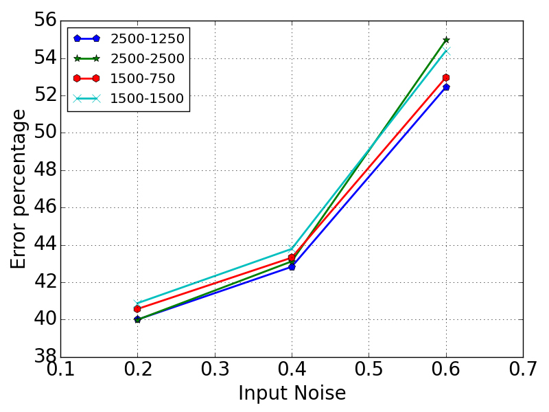
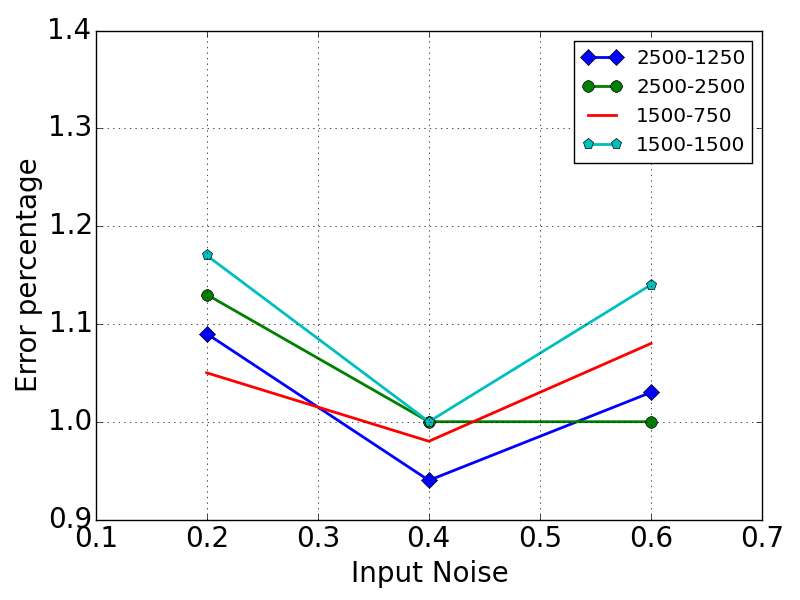
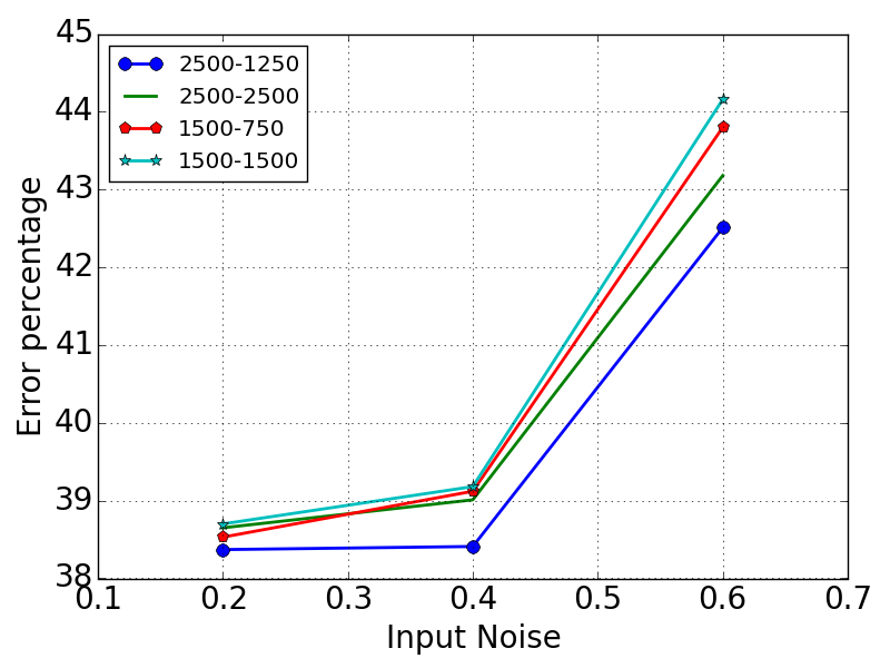
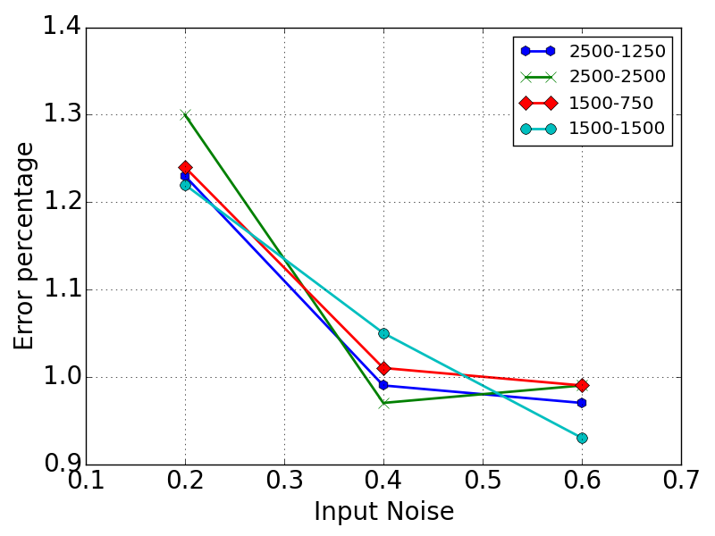
Figure 4: Error percentages on the MNIST and CIFAR-10 datasets using MLP architectures trained with different corruption schemes. Row-1: Experiments using dropout. Row-2: Experiments using noise back projection. Column-1: CIFAR-10 Column-2: MNIST.

Results suggest that Dropout can be replicated by projecting the noise back into the input and training a neural network deterministically on this generated data. There is not significant drop in accuracy, it is even slightly better than Dropout in the case of CIFAR-10. This supports the idea that dropout can be seen as data augmentation.

5.3 Richer noise schemes

We ran a series of experiments with fully connected feed forward neural networks on the MNIST and CIFAR-10 datasets to compare dropout. Each networks consist of two hidden layers with rectified linear units followed by a softmax layer. We experimented with three different network architectures each one with a different number of units in the hidden layers: 2500-625, 2500-1250 and 2500-2500. Each network is trained and validated the same way as mentioned in previous section.

First, we evaluated the dropout noise scheme by training the networks with a fixed hidden noise level of $0.5$ and the input noise level varying from $0.0$ to $0.7$ with increments of $0.1$ for each experiment. In the second experiment, we fixed the input noise level at $0.2$ and the hidden noise level is varied from $0.0$ to $0.7$, again with an increment of $0.1$. In the final set of experiments we use the random dropout noise scheme using the same noise level at input and hidden layers. The noise level in this case is a range $[0,x]$ where $x$ is varied from $0.0$ to $0.8$ with increment $0.1$. The classification performances corresponding to the all the experiments on both the datasets are reported in Figure 6.

Random dropout improves the performance of the models over dropout with no additional computational cost.

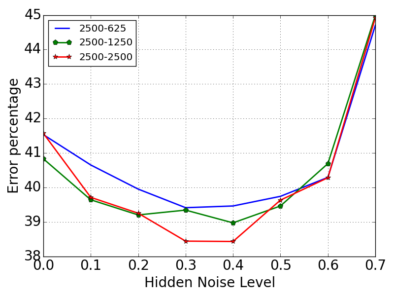
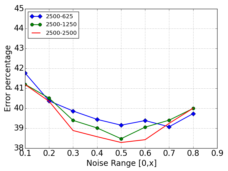
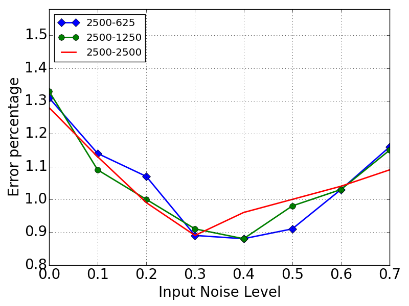
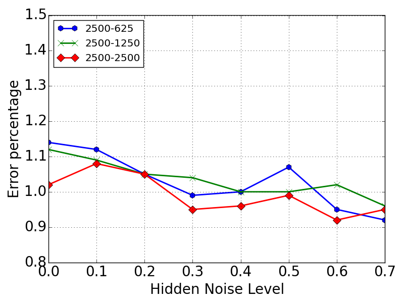
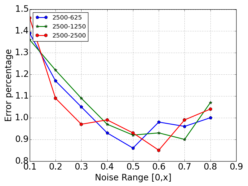
Figure 6: Error percentages on the MNIST and CIFAR-10 datasets using MLP architectures trained with different corruption schemes. Row-1: Experiments on CIFAR-10. Row-2: Experiments on MNIST. Column-1: Using dropout with varying input noise and fixed hidden noise of 0.5. Column-2: Using dropout with varying hidden noise with fixed input noise of 0.2. Column-3: Using Random-dropout with varying noise range $[0,x]$ used at hidden and input layers.

6 Related Work

To the best of our knowledge there is no work analyzing dropout from a data augmentation perspective. Nonetheless, there is a plethora of excellent works about dropout, some describing his regularisation properties and others developing new kind of noise schemes based on different intuitions.

Regularization properties of noise have been known for more than a decade, Bishop (1995) showed for instance that the regularization term induced by noise belongs to the class of generalized Tikhonov regularizers for sum-of-squares error functions. More recently, Baldi & Sadowski (2013) proved that dropout noise scheme specifically applies a regularisation term very similar to usual weight decay.

Not exactly about regularization, but uncertainty, Gal & Ghahramani (2015) gave a very inspiring interpretation of dropout as a Bayesian approximation.

Different noise schemes are used by Poole et al. (2014) and applied at different positions in autoencoders; input, pre-activation and post-activations. They report better results than denoising autoencoders and also support that Gaussian noise yields better results than dropout on MNIST classification task.

Bachman et al. (2014) emphasise bagging interpretation of dropout and propose a generalization called pseudo-ensembles and a related regularizer which makes it possible to train semi-supervised networks.

Some recent work reports that noise level schedules, inspired by simulated annealing, help in supervised and unsupervised tasks (Geras & Sutton, 2014; Chandra & Sharma, 2014; Rennie et al., 2014). We propose an alternative that avoids a schedule and rather uses random noise levels such that the model cannot adapt to slowly changing noise distribution.

A similar approach of sampling the noise level was used in Geras & Sutton (2014) in the context of unsupervised learning using an autoencoder (on input not features). However, they show that the approach is not very useful in their case.

Finally, work by Graham et al. (2015) is related to random noise as both their submatrix multiplications and random noise level $\rho$ are inducing an independence between neurons of a single layer. They found that the independence is not to damageable if they use enough different submatrix patterns.

7 Conclusion

We have presented and justified a novel interpretation of dropout as prior-knowledge free data augmentation. We described a new procedure to generate samples by back projecting the dropout noise into the input space. Our results suggest neural networks can be trained without dropout on such noisy samples and still yield good results. Nonetheless, experiments should be performed on larger networks in order to determine whether this observation is just a particular property of relatively small networks. Furthermore, trained networks should be analyzed to determine if co-adaptation is still avoided when using per-layer noise back-projection on deep neural networks.

Presenting only random dropout, the list of possible substitute to dropout in this work is far from exhaustive. As described in section 4, important knobs to modify induced data augmentation by noise are model’s features and the noise scheme applied on them. Using semi-supervised cost can influence the implicit transformations by forcing the network to learn more general features. A network could also be trained on $x^{*}$ samples generated from another network, similarly to generative adverserial networks (Goodfellow et al., 2014a).

8 Appendix

8.1 Proof of $x^{*}$ unlikeliness

We can show, with a proof by contradiction, that it’s unlikely to find a single $x^{*}=x^{(1)^{*}}=x^{(2)^{*}}=\dots=x^{(n)^{*}}$ that minimizes well $L$.

By the associative property of function composition, we can rewrite equation 7

$$f^{(i)}(x^{*})=\left(a^{(i)}\circ h^{(i)}\right)\left(f^{(i-1)}\left(x^{*}\right)\right)$$ (11)

Suppose there exist an $x^{*}$ such that

$$\left(a^{(i)}\circ h^{(i)}\right)\left(f^{(i-1)}\left(x^{*}\right)\right) =\left(\tilde{a}^{(i)}\circ h^{(i)}\right)\left(\tilde{f}^{(i-1)}(x)\right)$$ (12)

$$\left(a^{(i-1)}\circ h^{(i-1)}\right)\left(f^{(i-2)}\left(x^{*}\right)\right) =\left(\tilde{a}^{(i-1)}\circ h^{(i-1)}\right)\left(\tilde{f}^{(i-2)}(x)\right)$$ (13)

Based on 11 and 13, we have that $f^{(i-1)}(x^{*})=\tilde{f}^{(i-1)}(x)$. The proof is concluded by replacing the latter in 12 and then expanding the composed functions.

$$\left(a^{(i)}\circ h^{(i)}\right)\left(f^{(i-1)}\left(x^{*}\right)\right) =\left(\tilde{a}^{(i)}\circ h^{(i)}\right)\left(f^{(i-1)}(x^{*})\right)$$

$$\mbox{rect}\left(h^{(i)}\left(f^{(i-1)}\left(x^{*}\right)\right)\right) =\vec{m}^{(i)}\odot\mbox{rect}\left(h^{(i)}\left(f^{(i-1)}\left(x^{*}\right)\right)\right)$$ (14)

Equation 14 can only be true if $\vec{m}^{(i)}$ does not apply any modification to $\mbox{rect}\left(h^{(i)}\left(f^{(i-1)}\left(x^{*}\right)\right)\right)$, that means $\vec{m}^{(i)}_{j}=1$ when $\mbox{rect}_{j}\left(h^{(i)}\left(f^{(i-1)}\left(x^{*}\right)\right)\right)>0$. It happens with a probability $p_{(i)}^{d_{(i)}s_{(i)}}$ where $p_{(i)}$ is the Bernoulli success probability, $d_{(i)}$ is the number of hidden units and $s_{(i)}$ is the mean sparsity level, i.e. mean percentage of active hidden units, of the $i$-th hidden layer. This probability is very low for standard hyper-parameters values. For instance, with $p_{(i)}=0.5$, $d_{(i)}=1000$ and $s_{(i)}=0.15$, the probability is as low as $10^{-47}$.

References

- Bachman et al. (2014) Bachman, Phil, Alsharif, Ouais, and Precup, Doina. Learning with pseudo-ensembles. In Advances in Neural Information Processing Systems, pp. 3365–3373, 2014.
- Baldi & Sadowski (2013) Baldi, Pierre and Sadowski, Peter J. Understanding dropout. In Advances in Neural Information Processing Systems, pp. 2814–2822, 2013.
- Bastien et al. (2012) Bastien, Frédéric, Lamblin, Pascal, Pascanu, Razvan, Bergstra, James, Goodfellow, Ian, Bergeron, Arnaud, Bouchard, Nicolas, Warde-Farley, David, and Bengio, Yoshua. Theano: new features and speed improvements. arXiv preprint arXiv:1211.5590, 2012.
- Bergstra et al. (2010) Bergstra, James, Breuleux, Olivier, Bastien, Frédéric, Lamblin, Pascal, Pascanu, Razvan, Desjardins, Guillaume, Turian, Joseph, Warde-Farley, David, and Bengio, Yoshua. Theano: a cpu and gpu math expression compiler. In Proceedings of the Python for scientific computing conference (SciPy), volume 4, pp. 3. Austin, TX, 2010.
- Bishop (1995) Bishop, Chris M. Training with noise is equivalent to tikhonov regularization. Neural computation, 7(1):108–116, 1995.
- Chandra & Sharma (2014) Chandra, B and Sharma, Rajesh Kumar. Adaptive noise schedule for denoising autoencoder. In Neural Information Processing, pp. 535–542. Springer, 2014.
- Ciresan et al. (2012) Ciresan, Dan, Meier, Ueli, and Schmidhuber, Jürgen. Multi-column deep neural networks for image classification. In Computer Vision and Pattern Recognition (CVPR), 2012 IEEE Conference on, pp. 3642–3649. IEEE, 2012.
- Gal & Ghahramani (2015) Gal, Yarin and Ghahramani, Zoubin. Dropout as a bayesian approximation: Representing model uncertainty in deep learning. arXiv preprint arXiv:1506.02142, 2015.
- Geras & Sutton (2014) Geras, Krzysztof J and Sutton, Charles. Scheduled denoising autoencoders. arXiv preprint arXiv:1406.3269, 2014.
- Goodfellow et al. (2014a) Goodfellow, Ian, Pouget-Abadie, Jean, Mirza, Mehdi, Xu, Bing, Warde-Farley, David, Ozair, Sherjil, Courville, Aaron, and Bengio, Yoshua. Generative adversarial nets. In Advances in Neural Information Processing Systems, pp. 2672–2680, 2014a.
- Goodfellow et al. (2014b) Goodfellow, Ian J, Shlens, Jonathon, and Szegedy, Christian. Explaining and harnessing adversarial examples. arXiv preprint arXiv:1412.6572, 2014b.
- Graham et al. (2015) Graham, Ben, Reizenstein, Jeremy, and Robinson, Leigh. Efficient batchwise dropout training using submatrices. arXiv preprint arXiv:1502.02478, 2015.
- Hinton et al. (2012) Hinton, Geoffrey E., Srivastava, Nitish, Krizhevsky, Alex, Sutskever, Ilya, and Salakhutdinov, Ruslan. Improving neural networks by preventing co-adaptation of feature detectors. CoRR, abs/1207.0580, 2012.
- Krizhevsky et al. (2012) Krizhevsky, Alex, Sutskever, Ilya, and Hinton, Geoffrey E. Imagenet classification with deep convolutional neural networks. In Advances in neural information processing systems, pp. 1097–1105, 2012.
- LeCun et al. (1998) LeCun, Yann, Bottou, Léon, Bengio, Yoshua, and Haffner, Patrick. Gradient-based learning applied to document recognition. Proceedings of the IEEE, 86(11):2278–2324, 1998.
- Poole et al. (2014) Poole, Ben, Sohl-Dickstein, Jascha, and Ganguli, Surya. Analyzing noise in autoencoders and deep networks. arXiv preprint arXiv:1406.1831, 2014.
- Rennie et al. (2014) Rennie, Steven, Goel, Vaibhava, and Thomas, Samuel. Annealed dropout training of deep networks. In Spoken Language Technology (SLT), IEEE Workshop on. IEEE, 2014.
- Simard et al. (2003) Simard, Patrice Y, Steinkraus, Dave, and Platt, John C. Best practices for convolutional neural networks applied to visual document analysis. In 2013 12th International Conference on Document Analysis and Recognition, volume 2, pp. 958–958. IEEE Computer Society, 2003.
- Srivastava et al. (2014) Srivastava, Nitish, Hinton, Geoffrey, Krizhevsky, Alex, Sutskever, Ilya, and Salakhutdinov, Ruslan. Dropout: A simple way to prevent neural networks from overfitting. The Journal of Machine Learning Research, 15(1):1929–1958, 2014.
- van Merriënboer et al. (2015) van Merriënboer, Bart, Bahdanau, Dzmitry, Dumoulin, Vincent, Serdyuk, Dmitriy, Warde-Farley, David, Chorowski, Jan, and Bengio, Yoshua. Blocks and fuel: Frameworks for deep learning. arXiv preprint arXiv:1506.00619, 2015.
- Vincent et al. (2008) Vincent, Pascal, Larochelle, Hugo, Bengio, Yoshua, and Manzagol, Pierre-Antoine. Extracting and composing robust features with denoising autoencoders. In Proceedings of the 25th international conference on Machine learning, pp. 1096–1103. ACM, 2008.
- Wan et al. (2013) Wan, Li, Zeiler, Matthew, Zhang, Sixin, Cun, Yann L, and Fergus, Rob. Regularization of neural networks using dropconnect. In Proceedings of the 30th International Conference on Machine Learning (ICML-13), pp. 1058–1066, 2013.
- Wiesenfeld et al. (1995) Wiesenfeld, Kurt, Moss, Frank, et al. Stochastic resonance and the benefits of noise: from ice ages to crayfish and squids. Nature, 373(6509):33–36, 1995.
- Yarom & Hounsgaard (2011) Yarom, Yosef and Hounsgaard, Jorn. Voltage fluctuations in neurons: signal or noise? Physiological reviews, 91(3):917–929, 2011.