Bianchi Type $I$ Cosmology in $f(R,T)$ Gravity

Abstract

This paper is devoted to investigate the exact solutions of Bianchi type $I$ spacetime in the context of $f(R,T)$ gravity [1], where $f(R,T)$ is an arbitrary function of Ricci scalar $R$ and trace of the energy momentum tensor $T$. For this purpose, we find two exact solutions using the assumption of constant deceleration parameter and variation law of Hubble parameter. The obtained solutions correspond to two different models of the universe. The physical behavior of these models is also discussed.

Keywords: $f(R,T)$ gravity, Bianchi type $I$, deceleration parameter.
PACS: 04.50.Kd.

1 Introduction

The most popular issue in the modern day cosmology is the current expansion of universe. It is now evident from observational and theoretical facts that our universe is in the phase of accelerated expansion [2]-[11]. The phenomenon of dark energy and dark matter is another topic of discussion [12]-[19]. It was Einstein who first gave the concept of dark energy and introduced the small positive cosmological constant. But after sometime, he remarked it as the biggest mistake in his life. However, it is now thought that the cosmological constant may be a suitable candidate for dark energy. Another proposal to justify the current expansion of universe comes from modified or alternative theories of gravity. $f(T)$ theory of gravity is one such example which has been recently developed. This theory is a generalized version of teleparallel gravity in which Weitzenböck connection is used instead of Levi-Civita connection. The interesting feature of the theory is that it may explain the current acceleration without involving dark energy. A considerable amount of work has been done in this theory so far [20]. Another interesting modified theory is $f(R)$ theory of gravity which involves a general function of Ricci scalar in standard Einstein-Hilbert Lagrangian. Some review articles [21] can be helpful to understand the theory.

Many authors have investigated $f(R)$ gravity in different contexts [22]-[35]. Spherically symmetric solutions are most commonly studied solutions due to their closeness to the nature. Multam$\ddot{a}$ki and Vilja [36] explored vacuum and perfect fluid solutions of spherically symmetric spacetime in metric version of this theory. They used the assumption of constant scalar curvature and found that the solutions corresponded to the already existing solutions in general relativity (GR). Noether symmetries have been used by Capozziello et al. [37] to study spherically symmetric solutions in $f(R)$ gravity. Similarly many interesting results have been found using spherical symmetry in $f(R)$ gravity [38]. Cylindrically symmetric vacuum and non-vacuum solutions have also been explored in this theory [39]. Sharif and Shamir [40] found plane symmetric solutions. The same authors [41] discussed the solutions of Bianchi types $I$ and $V$ cosmologies for vacuum and non-vacuum cases. Conserved quantities in $f(R)$ gravity via Noether symmetry approach have been recently calculated [42].

In a recent paper [1], Harko et al. proposed a new generalized theory known as $f(R,T)$ gravity. In this theory, gravitational Lagrangian involves an arbitrary function of the scalar curvature $R$ and the trace of the energy momentum tensor $T$. Myrzakulov [43] discussed $f(R,T)$ gravity in which he explicitly presented point like Lagrangians. Sharif and Zubair [44] studied the laws of thermodynamics in this theory. The same authors [45] investigated holographic and agegraphic $f(R,T)$ models. Houndjo [46] reconstructed $f(R,T)$ gravity by taking $f(R,T)=f_{1}(R)+f_{2}(T)$ and it was proved that $f(R,T)$ gravity allowed transition of matter from dominated phase to an acceleration phase. Thus it is hoped that $f(R,T)$ gravity may explain the resent phase of cosmic acceleration of our universe. This theory can be used to explore many issues and may provide some satisfactory results.

The isotropic models are considered to be most suitable to study large scale structure of the universe. However, it is believed that the early universe may not have been exactly uniform. This prediction motivates us to describe the early stages of the universe with the models having anisotropic background. Thus, the existence of anisotropy in early phases of the universe is an interesting phenomenon to investigate. A Bianchi Type $I$ cosmological model, being the generalization of flat Friedmann-Robertson-Walker (FRW) model, is one of the simplest models of the anisotropic universe. Therefore, it seems interesting to explore Bianchi type models in the context of $f(R,T)$ gravity. Adhav [47] investigated the exact solutions of $f(R,T)$ field equations for locally rotationally symmetric Bianchi type $I$ spacetime. Reddy et al. [48] explored the solutions of Bianchi type $III$ spacetime using the law of variation of Hubble’s parameter. Bianchi type $III$ dark energy model in the presence of perfect fluid source has been reported [49]. Ahmed and Pradhan [50] studied Bianchi Type $V$ cosmology in this theory by involving the cosmological constant in the field equations. Naidu et al. [51] gave the solutions of Bianchi type $V$ bulk viscous string cosmological model.

In this paper, we are focussed to investigate the exact solutions of Bianchi type $I$ spacetime in the framework of $f(R,T)$ gravity. The plan of paper is as follows: In section 2, we give some basics of $f(R,T)$ gravity. Section 3 provides the exact solutions for Bianchi type $I$ spacetime. Concluding remarks are given in the last section.

2 Some Basics of $f(R,T)$ Gravity

The $f(R,T)$ theory of gravity is the generalization or modification of GR. The action for this theory is given by [1]

$$S=\int\sqrt{-g}\bigg{(}\frac{1}{16\pi{G}}f(R,T)+L_{m}\bigg{)}d^{4}x,$$ (1)

where $f(R,T)$ is an arbitrary function of the Ricci scalar $R$ and the trace $T$ of energy momentum tensor $T_{\mu\nu}$ while $L_{m}$ is the usual matter Lagrangian. It is worth mentioning that if we replace $f(R,T)$ with $f(R)$, we get the action for $f(R)$ gravity and replacement of $f(R,T)$ with $R$ leads to the action of GR. The energy momentum tensor $T_{\mu\nu}$ is defined as [52]

$$T_{\mu\nu}=-\frac{2}{\sqrt{-g}}\frac{\delta(\sqrt{-g}L_{m})}{\delta g^{\mu\nu}}.$$ (2)

Here we assume that the dependance of matter Lagrangian is merely on the metric tensor $g_{\mu\nu}$ rather than its derivatives. In this case, we get

$$T_{\mu\nu}=L_{m}g_{\mu\nu}-2\frac{\delta L_{m}}{\delta g^{\mu\nu}}.$$ (3)

The $f(R,T)$ gravity field equations are obtained by varying the action $S$ in Eq.(1) with respect to the metric tensor $g_{\mu\nu}$

$$f_{R}(R,T)R_{\mu\nu}-\frac{1}{2}f(R,T)g_{\mu\nu}-(\nabla_{\mu}\nabla_{\nu}-g_{\mu\nu}\Box)f_{R}(R,T)=\kappa T_{\mu\nu}-f_{T}(R,T)(T_{\mu\nu}+\Theta_{\mu\nu}),$$ (4)

where $\nabla_{\mu}$ denotes the covariant derivative and

$$\Box\equiv\nabla^{\mu}\nabla_{\mu},~{}~{}f_{R}(R,T)=\frac{\partial f_{R}(R,T)}{\partial R},~{}~{}f_{T}(R,T)=\frac{\partial f_{R}(R,T)}{\partial T},~{}~{}\Theta_{\mu\nu}=g^{\alpha\beta}\frac{\delta T_{\alpha\beta}}{\delta g^{\mu\nu}}.$$

Contraction of (4) yields

$$f_{R}(R,T)R+3\Box f_{R}(R,T)-2f(R,T)=\kappa T-f_{T}(R,T)(T+\Theta),$$ (5)

where $\Theta={\Theta_{\mu}}^{\mu}$. This is an important equation because it provides a relationship between Ricci scalar $R$ and the trace $T$ of energy momentum tensor. Using matter Lagrangian $L_{m}$, the standard matter energy-momentum tensor is derived as

$$T_{\mu\nu}=(\rho+p)u_{\mu}u_{\nu}-pg_{\mu\nu},$$ (6)

where $u_{\mu}=\sqrt{g_{00}}(1,0,0,0)$ is the four-velocity in co-moving coordinates and $\rho$ and $p$ denote energy density and pressure of the fluid respectively. Perfect fluids problems involving energy density and pressure are not any easy task to deal with. Moreover, there does not exist any unique definition for matter Lagrangian. Thus we can assume the matter Lagrangian as $L_{m}=-p$ which gives

$$\Theta_{\mu\nu}=-pg_{\mu\nu}-2T_{\mu\nu},$$ (7)

and consequently the field equations (4) take the form

$$f_{R}(R,T)R_{\mu\nu}-\frac{1}{2}f(R,T)g_{\mu\nu}-(\nabla_{\mu}\nabla_{\nu}-g_{\mu\nu}\Box)f_{R}(R,T)=\kappa T_{\mu\nu}+f_{T}(R,T)(T_{\mu\nu}+pg_{\mu\nu}),$$ (8)

It is mentioned here that these field equations depend on the physical nature of matter field. Many theoretical models corresponding to different matter contributions for $f(R,T)$ gravity are possible. However, Harko et al. [1] gave three classes of these models

$$f(R,T)=\left\{\begin{array}[]{c l}{R+2f(T),}\\ {f_{1}(R)+f_{2}(T),}\\ {f_{1}(R)+f_{2}(R)f_{3}(T).}\end{array}\right.$$

In this paper we are focussed to the first class, i.e. $f(R,T)=R+2f(T)$. For this model the field equations become

$$R_{\mu\nu}-\frac{1}{2}Rg_{\mu\nu}=\kappa T_{\mu\nu}+2f^{\prime}(T)T_{\mu\nu}+\bigg{[}f(T)+2pf^{\prime}(T)\bigg{]}g_{\mu\nu},$$ (9)

where prime represents derivative with respect to $T$.

3 Exact Solutions of Bianchi Type $I$ Universe

In this section, we shall find exact solutions of Bianchi I spacetime in $f(R,T)$ gravity. For the sake of simplicity, we use natural system of units $(G=c=1)$ and $f(T)=\lambda T$, where $\lambda$ is an arbitrary constant. For Bianchi type $I$ spacetime, the line element is given by

$$ds^{2}=dt^{2}-A^{2}(t)dx^{2}-B^{2}(t)dy^{2}-C^{2}(t)dz^{2},$$ (10)

where $A,~{}B$ and $C$ are defined as cosmic scale factors. The Bianchi $I$ Ricci scalar turns out to be

$$R=-2\bigg{[}\frac{\ddot{A}}{A}+\frac{\ddot{B}}{B}+\frac{\ddot{C}}{C}+\frac{\dot{A}\dot{B}}{AB}+\frac{\dot{B}\dot{C}}{BC}+\frac{\dot{C}\dot{A}}{CA}\bigg{]},$$ (11)

where dot denotes derivative with respect to $t$.

Using Eq.(9), we get four independent field equations,

$$\frac{\dot{A}\dot{B}}{AB}+\frac{\dot{B}\dot{C}}{BC}+\frac{\dot{C}\dot{A}}{CA}=(8\pi+3\lambda)\rho-\lambda p,$$ (12)

$$\frac{\ddot{B}}{B}+\frac{\ddot{C}}{C}+\frac{\dot{B}\dot{C}}{BC}=\lambda\rho-(8\pi+3\lambda)p,$$ (13)

$$\frac{\ddot{C}}{C}+\frac{\ddot{A}}{A}+\frac{\dot{C}\dot{A}}{AC}=\lambda\rho-(8\pi+3\lambda)p,$$ (14)

$$\frac{\ddot{A}}{A}+\frac{\ddot{B}}{B}+\frac{\dot{A}\dot{B}}{AB}=\lambda\rho-(8\pi+3\lambda)p.$$ (15)

These are four non-linear differential equations with five unknowns namely $A,~{}B,~{}C$, $\rho$ and $p$. Subtracting Eq.(14) from Eq.(13), Eq.(15) from Eq.(14) and Eq.(15) from Eq.(12), we get respectively

$$\frac{\ddot{A}}{A}-\frac{\ddot{B}}{B}+\frac{\dot{C}}{C}\bigg{(}\frac{\dot{A}}{A}-\frac{\dot{B}}{B}\bigg{)}=0,$$ (16)

$$\frac{\ddot{B}}{B}-\frac{\ddot{C}}{C}+\frac{\dot{A}}{A}\bigg{(}\frac{\dot{B}}{B}-\frac{\dot{C}}{C}\bigg{)}=0,$$ (17)

$$\frac{\ddot{A}}{A}-\frac{\ddot{C}}{C}+\frac{\dot{B}}{B}\bigg{(}\frac{\dot{A}}{A}-\frac{\dot{C}}{C}\bigg{)}=0.$$ (18)

These equations imply that

$$\frac{B}{A}=d_{1}\exp\bigg{[}{c_{1}\int\frac{dt}{a^{3}}}\bigg{]},$$ (19)

$$\frac{C}{B}=d_{2}\exp\bigg{[}{c_{2}\int\frac{dt}{a^{3}}}\bigg{]},$$ (20)

$$\frac{A}{C}=d_{3}\exp\bigg{[}{c_{3}\int\frac{dt}{a^{3}}}\bigg{]},$$ (21)

where $c_{1},~{}c_{2},~{}c_{3}$ and $d_{1},~{}d_{2},~{}d_{3}$ are integration constants which satisfy the following relation

$$c_{1}+c_{2}+c_{3}=0,\quad d_{1}d_{2}d_{3}=1.$$ (22)

Using Eqs.(19)-(21), we can write the unknown metric functions in an explicit way

$$A=ap_{1}\exp\bigg{[}{q_{1}\int\frac{dt}{a^{3}}}\bigg{]},$$ (23)

$$B=ap_{2}\exp\bigg{[}{q_{2}\int\frac{dt}{a^{3}}}\bigg{]},$$ (24)

$$C=ap_{3}\exp\bigg{[}{q_{3}\int\frac{dt}{a^{3}}}\bigg{]},$$ (25)

where

$$p_{1}=({d_{1}}^{-2}{d_{2}}^{-1})^{\frac{1}{3}},\quad p_{2}=(d_{1}{d_{2}}^{-1})^{\frac{1}{3}},\quad p_{3}=(d_{1}{d_{2}}^{2})^{\frac{1}{3}}$$ (26)

and

$$q_{1}=-\frac{2c_{1}+c_{2}}{3},\quad q_{2}=\frac{c_{1}-c_{2}}{3},\quad q_{3}=\frac{c_{1}+2c_{2}}{3}.$$ (27)

It is mentioned here that $p_{1},~{}p_{2},~{}p_{3}$ and $q_{1},~{}q_{2},~{}q_{3}$ also satisfy the relation

$$p_{1}p_{2}p_{3}=1,\quad q_{1}+q_{2}+q_{3}=0.$$ (28)

3.1 Some Important Physical Parameters

Now we present some important definitions of physical parameters. The average scale factor $a$ and volume scale factor $V$ are defined as

$$a=\sqrt[3]{ABC},\quad V=a^{3}=ABC.$$ (29)

The generalized mean Hubble parameter $H$ is given by

$$H=\frac{1}{3}(H_{1}+H_{2}+H_{3}),$$ (30)

where $H_{1}=\frac{\dot{A}}{A},~{}H_{2}=\frac{\dot{B}}{B},~{}H_{3}=\frac{\dot{C}}{C}$ are defined as the directional Hubble parameters in the directions of $x,~{}y$ and $z$ axis respectively. The mean anisotropy parameter $A$ is

$$A=\frac{1}{3}\sum^{3}_{i=1}\bigg{(}\frac{H_{i}-H}{H}\bigg{)}^{2}.$$ (31)

The expansion scalar $\theta$ and shear scalar $\sigma^{2}$ are defined as follows

$$\theta = u^{\mu}_{;\mu}=\frac{\dot{A}}{A}+\frac{\dot{B}}{B}+\frac{\dot{C}}{C},$$ (32)

$$\sigma^{2} = \frac{1}{2}\sigma_{\mu\nu}\sigma^{\mu\nu}=\frac{1}{3}\bigg{[}\bigg{(}\frac{\dot{A}}{A}\bigg{)}^{2}+\bigg{(}\frac{\dot{B}}{B}\bigg{)}^{2}+\bigg{(}\frac{\dot{C}}{C}\bigg{)}^{2}-\frac{\dot{A}\dot{B}}{AB}-\frac{\dot{B}\dot{C}}{BC}-\frac{\dot{C}\dot{A}}{CA}\bigg{]},~{}~{}$$ (33)

where

$$\sigma_{\mu\nu}=\frac{1}{2}(u_{\mu;\alpha}h^{\alpha}_{\nu}+u_{\nu;\alpha}h^{\alpha}_{\mu})-\frac{1}{3}\theta h_{\mu\nu}$$ (34)

with $h_{\mu\nu}=g_{\mu\nu}-u_{\mu}u_{\nu}$ defined as the projection tensor. The deceleration parameter $q$ is the measure of the cosmic accelerated expansion of the universe. It is defined as

$$q=-\frac{\ddot{a}a}{\dot{a}^{2}}.$$ (35)

The behavior of the universe models is determined by the sign of $q$. The positive value of deceleration parameter suggests a decelerating model while the negative value indicates inflation. Since there are four equations (12)-(15) and five unknowns, so we need an additional constraint to solve them. Here we use a well-known relation [53] between the average scale factor $a$ and Hubble parameter $H$ to solve the equations,

$$H=la^{-n},$$ (36)

where $l$ and $n$ are positive constants. This is an important relation because it yields a constant value of deceleration parameter and consequently we obtain power law and exponential models of universe. Using Eqs.(30) and (36), we get

$$\dot{a}=la^{1-n}$$ (37)

and the deceleration parameter becomes

$$q=n-1.$$ (38)

Integrating Eq.(37), it follows that

$$a=(nlt+k_{1})^{\frac{1}{n}},\quad n\neq 0,$$ (39)

and

$$a=k_{2}\exp(lt),\quad~{}~{}~{}n=0,$$ (40)

where $k_{1}$ and $k_{2}$ are constants of integration.

3.2 Singular Model of the Universe

Here we investigate the model of universe when $n\neq 0$, i.e., $a=(nlt+k_{1})^{\frac{1}{n}}$. In this case, the metric coefficients $A,~{}B$ and $C$ take the form

$$A = p_{1}(nlt+k_{1})^{\frac{1}{n}}\exp\bigg{[}\frac{q_{1}(nlt+k_{1})^{\frac{n-3}{n}}}{l(n-3)}\bigg{]},\quad n\neq 3,$$ (41)

$$B = p_{2}(nlt+k_{1})^{\frac{1}{n}}\exp\bigg{[}\frac{q_{2}(nlt+k_{1})^{\frac{n-3}{n}}}{l(n-3)}\bigg{]},\quad n\neq 3,$$ (42)

$$C = p_{3}(nlt+k_{1})^{\frac{1}{n}}\exp\bigg{[}\frac{q_{3}(nlt+k_{1})^{\frac{n-3}{n}}}{l(n-3)}\bigg{]},\quad n\neq 3.$$ (43)

The directional Hubble parameters $H_{i}$ ($i=1,2,3$) turn out to be

$$H_{i}=\frac{l}{nlt+k_{1}}+\frac{q_{i}}{(nlt+k_{1})^{\frac{3}{n}}}.$$ (44)

The mean generalized Hubble parameter and volume scale factor are

$$H=\frac{l}{nlt+k_{1}},\quad V=(nlt+k_{1})^{\frac{3}{n}}.$$ (45)

The mean anisotropy parameter becomes

$$A=\frac{{q_{1}}^{2}+{q_{2}}^{2}+{q_{3}}^{2}}{3l^{2}(nlt+k_{1})^{(6-2n)/n}}.$$ (46)

The expansion scalar and shear scalar for this model are given by

$$\theta=\frac{3l}{nlt+k_{1}},\quad\sigma^{2}=\frac{{q_{1}}^{2}+{q_{2}}^{2}+{q_{3}}^{2}}{2(nlt+k_{1})^{6/n}}.$$ (47)

Using Eqs. (12)-(15), the energy density of the universe turns out to be

$$\rho= \frac{1}{12(\lambda+2\pi)(\lambda+4\pi)}\bigg{[}4(\lambda+3\pi)\bigg{\{}\frac{3l^{2}}{(nlt+k_{1})^{2}}+\frac{q_{1}q_{2}+q_{2}q_{3}+q_{3}q_{1}}{(nlt+k_{1})^{\frac{6}{n}}}\bigg{\}}$$ (48)

$$- \lambda\bigg{\{}\frac{3l^{2}(1-n)}{(nlt+k_{1})^{2}}+\frac{{q_{1}}^{2}+{q_{2}}^{2}+{q_{3}}^{2}}{(nlt+k_{1})^{\frac{6}{n}}}\bigg{\}}\bigg{]}$$

while the pressure of the universe becomes

$$p= \frac{-1}{12(\lambda+2\pi)(\lambda+4\pi)}\bigg{[}4\pi\bigg{\{}\frac{3l^{2}}{(nlt+k_{1})^{2}}+\frac{q_{1}q_{2}+q_{2}q_{3}+q_{3}q_{1}}{(nlt+k_{1})^{\frac{6}{n}}}\bigg{\}}$$ (49)

$$+ (3\lambda+8\pi)\bigg{\{}\frac{3l^{2}(1-n)}{(nlt+k_{1})^{2}}+\frac{{q_{1}}^{2}+{q_{2}}^{2}+{q_{3}}^{2}}{(nlt+k_{1})^{\frac{6}{n}}}\bigg{\}}\bigg{]}.$$

The plots of $\rho$, $p$ and equation of state parameter $w=p/\rho$ against time coordinate $t$ are shown in figure $1$ and $2$ respectively. It is evident from figure $2$ that $w\rightarrow\frac{1}{3}$ as $t\rightarrow\infty$. Thus the model corresponds to a radiation dominated universe as the time grows.

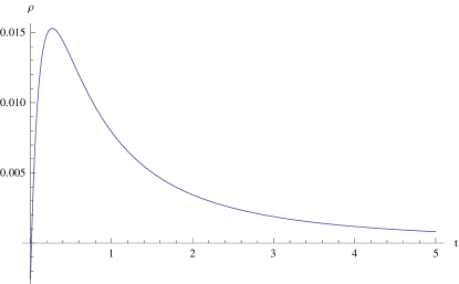
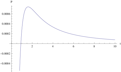
Figure 1: Behavior of energy density and pressure versus time for $t>0$ with $n=2,~{}\lambda=1,~{}l=1,~{}k_{1}=0,~{}q_{1}=1=q_{2}$ and $q_{3}=-2$.

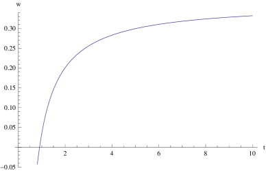
Figure 2: Behavior of $w$ versus time for $t>0$ with $n=2,~{}\lambda=1,~{}l=1,~{}k_{1}=0,~{}q_{1}=1=q_{2}$ and $q_{3}=-2$.

3.3 Non-singular Model of the Universe

For this model, $n=0$ and the average scale factor $a=k_{2}\exp(lt)$ turns the metric coefficients $A,~{}B$ and $C$ into

$$A = p_{1}k_{2}\exp(lt)\exp\bigg{[}-\frac{q_{1}\exp(-3lt)}{3l{k_{2}}^{3}}\bigg{]},$$ (50)

$$B = p_{2}k_{2}\exp(lt)\exp\bigg{[}-\frac{q_{2}\exp(-3lt)}{3l{k_{2}}^{3}}\bigg{]},$$ (51)

$$C = p_{3}k_{2}\exp(lt)\exp\bigg{[}-\frac{q_{3}\exp(-3lt)}{3l{k_{2}}^{3}}\bigg{]}.$$ (52)

The directional Hubble parameters $H_{i}$ become

$$H_{i}=l+\frac{q_{i}}{{k_{2}}^{3}}\exp(-3lt).$$ (53)

The mean generalized Hubble parameter and volume scale factor turn out to be

$$H=l,\quad V={k_{2}}^{3}\exp(3lt).$$ (54)

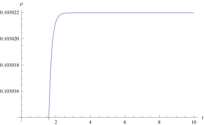
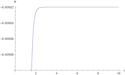
Figure 3: Behavior of energy density and pressure versus time for $t>0$ with $n=2,~{}\lambda=1,~{}l=1,~{}k_{2}=1,~{}q_{1}=1=q_{2}$ and $q_{3}=-2$.

The mean anisotropy parameter, expansion scalar and shear scalar are

$$A=\frac{{q_{1}}^{2}+{q_{2}}^{2}+{q_{3}}^{2}}{3l^{2}{k_{2}}^{6}\exp(6lt)},~{}~{}\theta=3l,\quad\sigma^{2}=\frac{{q_{1}}^{2}+{q_{2}}^{2}+{q_{3}}^{2}}{2{k_{2}}^{6}\exp(6lt)}.$$ (55)

The energy density and pressure of the universe take the form

$$\rho= \frac{1}{12(\lambda+2\pi)(\lambda+4\pi)}\bigg{[}4(\lambda+3\pi)\bigg{\{}3l^{2}+\frac{q_{1}q_{2}+q_{2}q_{3}+q_{3}q_{1}}{{k_{2}}^{6}\exp(6lt)}\bigg{\}}$$ (56)

$$- \lambda\bigg{\{}3l^{2}+\frac{{q_{1}}^{2}+{q_{2}}^{2}+{q_{3}}^{2}}{{k_{2}}^{6}\exp(6lt)}\bigg{\}}\bigg{]},$$

$$p= \frac{-1}{12(\lambda+2\pi)(\lambda+4\pi)}\bigg{[}4\pi\bigg{\{}3l^{2}+\frac{q_{1}q_{2}+q_{2}q_{3}+q_{3}q_{1}}{{k_{2}}^{6}\exp(6lt)}\bigg{\}}$$ (57)

$$+ (3\lambda+8\pi)\bigg{\{}3l^{2}+\frac{{q_{1}}^{2}+{q_{2}}^{2}+{q_{3}}^{2}}{{k_{2}}^{6}\exp(6lt)}\bigg{\}}\bigg{]}.$$

For this model, the plots of $\rho$, $P$ and $w$ against time coordinate $t$ are shown in figure $3$ and $4$ respectively. It can be seen from figure $4$ that $w\rightarrow-1$ as $t\rightarrow\infty$ which indicates that the non-singular model corresponds to a vacuum fluid dominated universe.

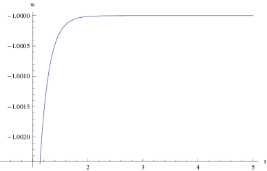
Figure 4: Behavior of $w$ versus time for $t>0$ with $~{}n=2,~{}\lambda=1,~{}l=1,~{}k_{2}=1,~{}q_{1}=1=q_{2}$ and $q_{3}=-2$.

4 Concluding Remarks

This paper is devoted to discuss the current phenomenon of accelerated expansion of universe in the framework of newly proposed $f(R,T)$ theory of gravity. For this purpose, we take $f(R,T)=R+2\lambda T$ and explore the exact solutions of Bianchi type $I$ cosmological model. We obtain two exact solutions using the assumption of constant value of deceleration parameter and the law of variation of Hubble parameter. The obtained solutions correspond to two different models of universe. The first solution forms a singular model with power law expansion while the second solution gives a non-singular model with exponential expansion of universe. The physical parameters for both of these models are discussed below.

The singular model of the universe corresponds to $n\neq 0$ with average scale factor $a=(nlt+k_{1})^{\frac{1}{n}}$. This model possesses a point singularity when $t\equiv t_{s}=-\frac{k_{1}}{nl}$. The volume scale factor and the metric coefficients $A,~{}B$ and $C$ vanish at this singularity point. The cosmological parameters $H_{1},~{}H_{2},~{}H_{3},~{}H,~{}\theta$, and $\sigma^{2}$ are all infinite at this point of singularity. If we choose $k_{1}=0$, figure $1$ suggests that energy density of the universe is zero at this time. The pressure approaches negative infinity as $t\rightarrow 0$. This strong negative pressure is an indication of dark energy. For this model, $w\rightarrow\frac{1}{3}$ as $t\rightarrow\infty$ which corresponds to a radiation dominated universe. The mean anisotropy parameter $A$ also becomes infinite at this point for $0<n<3$ and vanishes for $n>3$. Moreover, the isotropy condition, i.e., $\frac{\sigma^{2}}{\theta}\rightarrow 0$ as $t\rightarrow\infty$, is verified for this model. All these conclusive observations suggest that the universe starts its expansion with zero volume, strong negative pressure and energy density from $t=t_{s}$ and it will continue to expand for $0<n<3$.

Now we discuss the non-singular model of the universe corresponds to $n=0$. For this model the average scale factor is $a=k_{2}\exp(lt)$. The non-singularity is due to the exponential behavior of the model. The expansion scalar $\theta$ and mean generalized Hubble parameter $H$ are constant in this case. For finite values of $t$, the physical parameters $H_{1},~{}H_{2},~{}H_{3},~{}\sigma^{2}$ and $A$ are all finite. The metric functions are defined for finite time and the isotropy condition is satisfied. There is an exponential increase in the volume as the time grows. However, energy density is approximately zero initially and becomes constant after some time. Pressure of the universe remains in the negative zone for this model which may be an indication of presence of dark energy in the universe. Figure $4$ suggests that $w\rightarrow-1$ as $t\rightarrow\infty$. Thus the exponential model corresponds to a vacuum fluid dominated universe. According to the observations [54], the expansion of the universe is accelerating when $w\approx-1$.

Therefore, it is hoped that the problematic issues such as dark energy and accelerated expansion of universe may be addressed using modified theories of gravity especially $f(R,T)$ gravity. It would be interesting to explore more Bianchi type solutions in this context. Exact solutions of Bianchi type $V$ cosmological model in this theory are under process.

Acknowledgement

The author is thankful to National University of Computer and Emerging Sciences (NUCES) Lahore Campus for funding the PhD programme. The author is also grateful to the anonymous reviewer for valuable comments and suggestions to improve the paper.

References

- [1] Harko, T., Lobo, F.S.N., Nojiri, S. and Odintsov, S.D.: Phys. Rev. D84(2011)024020.
- [2] Riess, A.G. et al.: Astron. J. 116(1998)1009; Riess, A.G. et al.: Astrophys. J. 607(2004)665.
- [3] Perlmutter, S. et al.: Astrophys. J. 517(1999)565.
- [4] Carmeli, M.: Commun. Theor. Phys. 5(1996)159.
- [5] Seprgel, D. N. et al.: Astrophys. J. Suppl. 148(2003)175; Spergel, D.N. et al.: Astrophys. J. Suppl. 170(2007)377.
- [6] Allen, S. W. et al.: Mon. Not. R. Astron. Soc. 353(2004)457.
- [7] Bennett, C. L. et al.: Astrophys. J. 148(2003)1.
- [8] Hogan, J.: Nature 448(2007)240.
- [9] Tegmark, M. et al.: Phys. Rev. D69(2004)103501
- [10] Abazajian, K. et al.: Astron. J. 129(2005)1755.
- [11] Astier, P. et al.: Astron. Astrophys. 447(2006)31.
- [12] Nojiri, S. and Odintsov, S.D.: Int. J. Geom. Meth. Mod. Phys. 4(2007)115.
- [13] Turner, M.S., Huterer, D.: J. Phys. Soc. Jap. 76(2007)111015; Frieman, J., Turner, M. and Huterer, D.: Ann. Rev. Astron. Astrophys. 46(2008)385.
- [14] Li, M., Li, X.D., Wang, S. and Wang, Y.: Commun. Theor. Phys. 56(2011)525.
- [15] Copeland, E.J., Sami, M. and Tsujikawa, S.: Int. J. Mod. Phys. D15(2006)1753.
- [16] Sahni, V. and Starobinsky, A.: Int. J. Mod. Phys. D9 (2000) 373; Sahni, V.: Lect. Notes. Phys. 653 (2004) 141.
- [17] Carroll, S.M.: Living Rev. Rel. 4(2001)1.
- [18] Weinberg, D.H.: New. Astron. Rev. 49(2005)337.
- [19] Straumann, N.: Mod. Phys. Lett. A21(2006)1083.
- [20] Yang, R.J.: Europhys. Lett. 93(2011)60001; Wei, H., Ma, X.P. and Qi, H.Y.: Phys. Lett. B703(2011)74; Wu, P.X. and Yu, H.W.: Eur. Phys. J. C71(2011)1552; Wu, P.X. and Yu, H.W.: Phys. Lett. B703(2011)223; Bamba, K., Geng, C.Q., Lee, C.C and Luo, L.W.: JCAP 1101(2011)021; Li, B., Sotiriou, T.P. and Barrow, J.D.: Phys. Rev. D83(2011)104017.
- [21] Felice, A.D and Tsujikawa, S.: Living Rev. Rel. 13(2010)3; Sotiriou, T.P. and Faraoni, V.: Rev. Mod. Phys. 82(2010)451; Clifton, T., Ferreira, P.G., Padilla, A. and Skordis, C.: Phys. Rept. 513 (2012)1; Nojiri, S. and Odintsov, S.D.: Phys. Rept. 505(2011)59. Bamba, K., Capozziello, S., Nojiri, S. and Odintsov, S.D.: Astrophys. Space Sci. 342(2012)155.
- [22] Sharif, M. and Zubair, M.: Adv. High Energy Phys. 2013(2013)790967.
- [23] Sharif, M. and Kausar, H.R.: JCAP 07(2011)022.
- [24] Sharif, M. and Kausar, H.R.: Int. J. Mod. Phys. D20(2011)2239.
- [25] Sharif, M. and Kausar, H.R.: Astrophys. Space Sci. 331(2011)281.
- [26] Sharif, M. and Kausar, H.R.: Mod. Phys. Lett. A25(2010)3299.
- [27] Bamba, K., Nojiri, S., Odintsov, S.D. and Saez-Gomez, D.: Phys. Lett. B730(2014)136.
- [28] Bamba, K., Makarenko, A.N., Myagky, A.N., Nojiri, S. and Odintsov, S.D.: JCAP 01(2014)008.
- [29] Bamba, K., Nojiri, S. and Odintsov, S.D.: Phys. Lett. B698(2011)451.
- [30] Capozziello, S. and Vignolo, S.: Int. J. Geom. Meth. Mod. Phys. 8(2011)167.
- [31] Capozziello, S., Darabi, F. and Vernieri, D.: Mod. Phys. Lett. A26(2011)65.
- [32] Capozziello, S., Laurentis, M.D., Odintsov, S.D. and Stabile, A.: Phys. Rev. D83(2011)064004.
- [33] Elizalde, E., Nojiri, S., Odintsov, S.D. and Saez-Gomez, D.: Eur. Phys. J. C70(2010)351.
- [34] Bamba, K., Geng, C., Nojiri, S. and Odintsov, S.D.: Mod. Phys. Lett. A25(2010)900.
- [35] Capozziello, S., Laurentis, M.D., Nojiri, S. and Odintsov, S.D.: Gen. Rel. Grav. 41(2009)2313.
- [36] Multamki, T. and Vilja, I.: Phys. Rev. D74(2006)064022; Multamki, T. and Vilja, I.: Phys. Rev. D76(2007)064021.
- [37] Capozziello, S., Stabile, A. and Troisi, A.: Class. Quantum Grav. 24(2007)2153.
- [38] Hollenstein, L. and Lobo, F.S.N.: Phys. Rev. D78(2008)124007; Sharif, M. and Kausar, H.R.: J. Phys. Soc. Jpn. 80(2011)044004; Shojai, A. and Shojai, F.: Gen. Relativ. Gravit. 44(2011)211.
- [39] Azadi, A., Momeni, D. and Nouri-Zonoz, M.: Phys. Lett. B670(2008)210; Momeni, D. and Gholizade, H.: Int. J. Mod. Phys. D18(2009)1719; Sharif, M. and Arif, S.: Astrophys. Space Sci. 342(2012)237.
- [40] Sharif, M. and Shamir, M.F.: Mod. Phys. Lett. A25(2010)1281.
- [41] Sharif, M. and Shamir, M.F.: Class. Quantum Grav. 26(2009)235020; Sharif, M. and Shamir, M.F.: Gen. Relativ. Gravit. 42(2010)2643.
- [42] Shamir, M.F., Jhangeer, A. and Bhatti, A.A.: Chin. Phys. Lett. 29(8)(2012)080402.
- [43] Myrzakulov, R.: Phys. Rev. D84(2011)024020.
- [44] Sharif, M. and Zubair, M.: JCAP 03(2012)028.
- [45] Sharif, M. and Zubair, M.: J. Phys. Soc. Jpn. 82(2013)064001.
- [46] Houndjo, M.J.S.: Int. J. Mod. Phys. D21(2012)1250003.
- [47] Adhav, K.S.: Astrophys. Space Sci. 339(2012)365.
- [48] Reddy, D.R.K., Santikumar, R. and Naidu, R.L.: Astrophys. Space Sci. 342(2012)249.
- [49] Reddy, D.R.K., Santikumar, R. and Pradeepkumar, T.V.: Int. J. Theor. Phys. 52(2013)239.
- [50] Naidu, R.L., Reddy, D.R.K., Ramprasad, T. and Ramana, K.V.: Astrophys. Space Sci. 348(2013)247.
- [51] Ahmed, N. and Pradhan, A.: Int. J. Theor. Phys. 53(2014)289.
- [52] Landau, L.D. and Lifshitz E.M.: The Classical Theory of Fileds (Butterworth-Heinemann, 2002).
- [53] Berman, M.S.: Nuov. Cim. B74(1983)182; Shamir, M.F. and Bhatti, A.A.: Can. J. Phys. 90(2012)193; Singh, C.P. and Kumar, S.: Int. J. Theor. Phys. 47(2008)3171-3179; Singh, C.P., Zeyauddin, M. and Ram, S.: Int. J. Theor. Phys. 47(2008)3162-3170.
- [54] Hogan, J.: Nature 448(2007)240.