Dynamics of f​(R)𝑓𝑅f(R) gravity models and asymmetry of time

Murli Manohar Verma sunilmmv@yahoo.com    Bal Krishna Yadav balkrishnalko@gmail.com Department of Physics, University of Lucknow, Lucknow 226 007, India
Abstract

We solve the field equations of modified gravity for f​(R)𝑓𝑅f(R) model in metric formalism. Further, we obtain the fixed points of the dynamical system in phase space analysis of f​(R)𝑓𝑅f(R) models, both with and without the effects of radiation. Stability of these points is studied against perturbations in a smooth spatial background by applying the conditions on the eigenvalues of the matrix obtained in the linearized first-order differential equations. Following this, these fixed points are used for analysing the dynamics of the system during the radiation, matter and acceleration dominated phases of the universe. Certain linear and quadratic forms of f​(R)𝑓𝑅f(R) are determined from the geometrical and physical considerations and the behaviour of the scale factor is found for those forms. Further, we also determine the Hubble parameter H​(t)𝐻𝑑H(t), Ricci scalar R𝑅R for these cosmic phases. We show the emergence of an asymmetry of time from the dynamics of the scalar field exclusively owing to the f​(R)𝑓𝑅f(R) gravity in the Einstein frame that may lead to an arrow of time at a classical level.

pacs:
98.80.-k, 95.36.+x, 04.50.-h

I Introduction

The present state of the universe has been found to be in the phase of accelerated expansiona1 . There are several observational evidences on geometry and growth of structures such as the Supernovae Ia, Baryon Acoustic Osicllation (BAO), Cosmic Microwave Background anisotropies, weak gravitational lensing etc. a1 ; a2 ; a3 ; a4 which indicate the presence of a hitherto unknown dark energy. By all reckoning, the explanation for present accelerated expansion of the universe is a major challenge in cosmology, even though there are many approaches to explain its dynamics. The simplest candidate for dark energy is the cosmological constant with a constant equation of state (w=βˆ’1𝑀1w=-1) a5 . However, there are two main difficulties associated with the cosmological constant – (i) the fine tuning problem and (ii) the coincidence problem. Besides, there exist two basic approaches attmpting to explain dark energy. The first approach is based on modified matter models. In this approach Tμ​νsubscriptπ‘‡πœ‡πœˆT_{\mu\nu} in the Einstein equations must include an exotic matter component like quintessence, k-essence, Phantom energy etc. a6 ; a7 ; a8 ; a9 that takes the form of dark energy and so the resposibility of causing acceleration. The second approach is through the so-called modified gravity models wherein the late-time accelerated cosmic expansion is realized without requiring the explicit dark energy component in the universe. In these models, we have a wide range of f​(R)𝑓𝑅f(R) gravity a10 , scalar-tensor theories, Gauss-Bonnet models, braneworld models etc. a11 ; a12 ; a13 . Specifcally, in this paper we present an analysis of f​(R)𝑓𝑅f(R) models, where one modifies the laws of gravity by replacing the scalar curvature R𝑅R of the Hilbert’s action, or Rβˆ’2​Λ𝑅2Ξ›R-2\Lambda, as one includes in the standard ΛΛ\LambdaCDM approach (with ΛΛ\Lambda as the cosmological constant), by an arbitrary function of R𝑅R in the curvature part of the Lagrangian density. At present, there is no specific, known functional form of R𝑅R which may satisfy all the observational conditions of cosmological viability ranging from the radiation dominated matter to the ongoing accelerated phase. Therefore, we study the stability conditions for the respective eras and determine the corresponding forms of f​(R)𝑓𝑅f(R). By solving the field equations for different forms of f​(R)𝑓𝑅f(R), the scale factor of expansion is thus determined. From here we find the scalar curvature R𝑅R and compare them in different eras. This can lead to the determination of a time-ordering of various epochs, dominated by radiation, matter and dark energy (as a modification of gravity), respectively, throughout the evolution of the universe.

In section II, the fixed points of the dynamical system are determined within the framework of f​(R)𝑓𝑅f(R) models in metric formalism. To study the exclusive effects of radiation, in sections III and IV the properties and stability of the fixed points of the dynamical system are found without and with radiation. Section V comprises of analysis of the behaviour of f​(R)𝑓𝑅f(R), scale factor a​(t)π‘Žπ‘‘a(t), Hubble parameter H​(t)𝐻𝑑H(t) (under various conditions) and scalar curvature R𝑅R in radiation dominated phase. In sections VI and VII we attempt to determine the form of f​(R)𝑓𝑅f(R), scale factor a​(t)π‘Žπ‘‘a(t) and scalar curvature R𝑅R for matter dominated and the present accelerated expansion dominated phases, respectively. Together, the time ordering may be used further to determine an arrow of time through the cosmic evolution in section VIII. Finally, we conclude our results in section IX.

II Field equations and phase space dynamics

In f​(R)𝑓𝑅f(R) gravity we obtain the field equations in metric formalism, where the variation of the action is taken with respect to gμ​νsubscriptπ‘”πœ‡πœˆg_{\mu\nu} related to the connections Γβ​γαsubscriptsuperscriptΓ𝛼𝛽𝛾\Gamma^{\alpha}_{\beta\gamma} in the usual sense (unlike the Palatini formalism where they are treated as mutually independent). We consider the field equations in the background of spatially flat Friedmann-Lemaitre-Robertson-Walker (FLRW) spacetime with a metric

d​s2=βˆ’d​t2+a2​(t)​[d​r2+r2​(d​θ2+sin2⁑θ​d​ϕ2)]𝑑superscript𝑠2𝑑superscript𝑑2superscriptπ‘Ž2𝑑delimited-[]𝑑superscriptπ‘Ÿ2superscriptπ‘Ÿ2𝑑superscriptπœƒ2superscript2πœƒπ‘‘superscriptitalic-Ο•2\displaystyle ds^{2}=-dt^{2}+a^{2}(t)[dr^{2}+r^{2}(d\theta^{2}+\sin^{2}\theta d\phi^{2})] (1)

where a​(t)π‘Žπ‘‘a(t) is time dependent scale factor and the speed of light c=1𝑐1c=1. Correspondingly, the Ricci scalar R𝑅R is given by

R=6​(2​H2+HΛ™)𝑅62superscript𝐻2˙𝐻\displaystyle R=6(2H^{2}+\dot{H}) (2)

where H(=aΛ™/a)annotated𝐻absentΛ™π‘Žπ‘ŽH(=\dot{a}/a) is the Hubble parameter and an overdot represents the derivative with respect to time. The total action using an arbitrary function f​(R)𝑓𝑅f(R) in the Jordan frame is given by

π’œ=12​κ2β€‹βˆ«βˆ’g​f​(R)​d4​x+π’œmπ’œ12superscriptπœ…2𝑔𝑓𝑅superscript𝑑4π‘₯subscriptπ’œπ‘š\displaystyle\mathcal{A}=\frac{1}{2\kappa^{2}}\int\sqrt{-g}f(R)d^{4}x+\mathcal{A}_{m} (3)

where π’œmsubscriptπ’œπ‘š\mathcal{A}_{m} is the action for relativistic and non-relativistic matter, ΞΊ2=8​π​Gsuperscriptπœ…28πœ‹πΊ\kappa^{2}=8\pi G and g𝑔g is the determinant of the metric tensor gμ​νsubscriptπ‘”πœ‡πœˆg_{\mu\nu}. Varying the action (3) with respect to gμ​νsubscriptπ‘”πœ‡πœˆg_{\mu\nu}, the field equations obtained are

F​(R)​RΞΌβ€‹Ξ½βˆ’12​f​(R)​gμ​ν𝐹𝑅subscriptπ‘…πœ‡πœˆ12𝑓𝑅subscriptπ‘”πœ‡πœˆ\displaystyle F(R)R_{\mu\nu}-\frac{1}{2}f(R)g_{\mu\nu}
βˆ’βˆ‡ΞΌβˆ‡β‘Ξ½β€‹F​(R)+gμ​ν​░​F​(R)=ΞΊ2​Tμ​ν,subscriptβˆ‡πœ‡βˆ‡πœˆπΉπ‘…subscriptπ‘”πœ‡πœˆβ–‘πΉπ‘…superscriptπœ…2subscriptπ‘‡πœ‡πœˆ\displaystyle-\nabla_{\mu}\nabla\nu F(R)+g_{\mu\nu}\Box F(R)=\kappa^{2}T_{\mu\nu}, (4)

where F​(R)β‰‘βˆ‚fβˆ‚R𝐹𝑅𝑓𝑅F(R)\equiv\frac{\partial{f}}{\partial{R}} and Tμ​νsubscriptπ‘‡πœ‡πœˆT_{\mu\nu} is the energy-momentum tensor for matter. From the above equation (4) and its trace we arrive at the the following ones

3​F​H2=ΞΊ2​(ρm+ρr)+(F​Rβˆ’f)2βˆ’3​H​FΛ™3𝐹superscript𝐻2superscriptπœ…2subscriptπœŒπ‘šsubscriptπœŒπ‘ŸπΉπ‘…π‘“23𝐻˙𝐹\displaystyle 3FH^{2}=\kappa^{2}(\rho_{m}+\rho_{r})+\frac{(FR-f)}{2}-3H\dot{F} (5)
βˆ’2​F​HΛ™=ΞΊ2​(ρm+43​ρr)+FΒ¨βˆ’H​FΛ™2𝐹˙𝐻superscriptπœ…2subscriptπœŒπ‘š43subscriptπœŒπ‘ŸΒ¨πΉπ»Λ™πΉ\displaystyle-2F\dot{H}=\kappa^{2}(\rho_{m}+\frac{4}{3}\rho_{r})+\ddot{F}-H\dot{F} (6)

where ρmsubscriptπœŒπ‘š\rho_{m} and ρrsubscriptπœŒπ‘Ÿ\rho_{r} are the energy densities of matter and radiation, respectively.

With four (dimensionless) variables defined as

x1β‰‘βˆ’FΛ™F​Hsubscriptπ‘₯1˙𝐹𝐹𝐻\displaystyle x_{1}\equiv-\frac{\dot{F}}{FH} (7)
x2β‰‘βˆ’f6​F​H2subscriptπ‘₯2𝑓6𝐹superscript𝐻2\displaystyle x_{2}\equiv-\frac{f}{6FH^{2}} (8)
x3≑R6​H2subscriptπ‘₯3𝑅6superscript𝐻2\displaystyle x_{3}\equiv\frac{R}{6H^{2}} (9)
x4≑κ2​ρr3​F​H2subscriptπ‘₯4superscriptπœ…2subscriptπœŒπ‘Ÿ3𝐹superscript𝐻2\displaystyle x_{4}\equiv\frac{\kappa^{2}\rho_{r}}{3FH^{2}} (10)

the effective equation of state for this system is defined by

we​f​f=βˆ’1βˆ’23​HΛ™H2=βˆ’13​(2​x3βˆ’1)subscript𝑀𝑒𝑓𝑓123˙𝐻superscript𝐻2132subscriptπ‘₯31\displaystyle w_{eff}=-1-\frac{2}{3}\frac{\dot{H}}{H^{2}}=-\frac{1}{3}(2x_{3}-1) (11)

Differentiation of these variables (7-10) with respect to N=ln⁑a​(t)π‘π‘Žπ‘‘N=\ln a(t) gives

d​x1d​N=βˆ’1βˆ’x3βˆ’3​x2+x12βˆ’x1​x3+x4𝑑subscriptπ‘₯1𝑑𝑁1subscriptπ‘₯33subscriptπ‘₯2superscriptsubscriptπ‘₯12subscriptπ‘₯1subscriptπ‘₯3subscriptπ‘₯4\displaystyle\frac{dx_{1}}{dN}=-1-x_{3}-3x_{2}+x_{1}^{2}-x_{1}x_{3}+x_{4} (12)
d​x2d​N=x1​x3mβˆ’x2​(2​x3βˆ’4βˆ’x1)𝑑subscriptπ‘₯2𝑑𝑁subscriptπ‘₯1subscriptπ‘₯3π‘šsubscriptπ‘₯22subscriptπ‘₯34subscriptπ‘₯1\displaystyle\frac{dx_{2}}{dN}=\frac{x_{1}x_{3}}{m}-x_{2}(2x_{3}-4-x_{1}) (13)
d​x3d​N=βˆ’x1​x3mβˆ’2​x3​(x3βˆ’2)𝑑subscriptπ‘₯3𝑑𝑁subscriptπ‘₯1subscriptπ‘₯3π‘š2subscriptπ‘₯3subscriptπ‘₯32\displaystyle\frac{dx_{3}}{dN}=-\frac{x_{1}x_{3}}{m}-2x_{3}(x_{3}-2) (14)
d​x4d​N=βˆ’2​x3​x4+x1​x4𝑑subscriptπ‘₯4𝑑𝑁2subscriptπ‘₯3subscriptπ‘₯4subscriptπ‘₯1subscriptπ‘₯4\displaystyle\frac{dx_{4}}{dN}=-2x_{3}x_{4}+x_{1}x_{4} (15)

where

m≑d​log⁑Fd​log⁑R=R​f,RRf,R,\displaystyle m\equiv\frac{d\log F}{d\log R}=\frac{Rf_{,RR}}{f_{,R}}, (16)
qβ‰‘βˆ’d​log⁑fd​log⁑R=βˆ’R​f,Rf=x3x2\displaystyle q\equiv-\frac{d\log f}{d\log R}=-\frac{Rf_{,R}}{f}=\frac{x_{3}}{x_{2}} (17)

where f,R≑d​fd​Rf_{,R}\equiv\frac{df}{dR} and f,RR≑d2​fd​R2f_{,RR}\equiv\frac{d^{2}f}{dR^{2}}. The fixed points of the system are obtained by equating the equations (12 - 15) to zero. Thus, the points are given by

P1:(x1,x2,x3,x4)=(0,βˆ’1,2,0),:subscript𝑃1subscriptπ‘₯1subscriptπ‘₯2subscriptπ‘₯3subscriptπ‘₯40120\displaystyle P_{1}:(x_{1},x_{2},x_{3},x_{4})=(0,-1,2,0),
Ξ©m=0,we​f​f=βˆ’1formulae-sequencesubscriptΞ©π‘š0subscript𝑀𝑒𝑓𝑓1\displaystyle\Omega_{m}=0,w_{eff}=-1 (18)
P2:(x1,x2,x3,x4)=(βˆ’1,0,0,0),:subscript𝑃2subscriptπ‘₯1subscriptπ‘₯2subscriptπ‘₯3subscriptπ‘₯41000\displaystyle P_{2}:(x_{1},x_{2},x_{3},x_{4})=(-1,0,0,0),
Ξ©m=2,we​f​f=13formulae-sequencesubscriptΞ©π‘š2subscript𝑀𝑒𝑓𝑓13\displaystyle\Omega_{m}=2,w_{eff}=\frac{1}{3} (19)
P3:(x1,x2,x3,x4)=(1,0,0,0),:subscript𝑃3subscriptπ‘₯1subscriptπ‘₯2subscriptπ‘₯3subscriptπ‘₯41000\displaystyle P_{3}:(x_{1},x_{2},x_{3},x_{4})=(1,0,0,0),
Ξ©m=0,we​f​f=13formulae-sequencesubscriptΞ©π‘š0subscript𝑀𝑒𝑓𝑓13\displaystyle\Omega_{m}=0,w_{eff}=\frac{1}{3} (20)
P4:(x1,x2,x3,x4)=(βˆ’4,5,0,0),:subscript𝑃4subscriptπ‘₯1subscriptπ‘₯2subscriptπ‘₯3subscriptπ‘₯44500\displaystyle P_{4}:(x_{1},x_{2},x_{3},x_{4})=(-4,5,0,0),
Ξ©m=0,we​f​f=13,formulae-sequencesubscriptΞ©π‘š0subscript𝑀𝑒𝑓𝑓13\displaystyle\Omega_{m}=0,w_{eff}=\frac{1}{3}, (21)
P5:(x1,x2,x3,x4)=:subscript𝑃5subscriptπ‘₯1subscriptπ‘₯2subscriptπ‘₯3subscriptπ‘₯4absent\displaystyle P_{5}:(x_{1},x_{2},x_{3},x_{4})=
(3​m1+m,βˆ’1+4​m2​(1+m)2,1+4​m2​(1+m),0),3π‘š1π‘š14π‘š2superscript1π‘š214π‘š21π‘š0\displaystyle(\frac{3m}{1+m},-\frac{1+4m}{2(1+m)^{2}},\frac{1+4m}{2(1+m)},0),
Ξ©m=1βˆ’m​(7+10​m)2​(1+m)2,subscriptΞ©π‘š1π‘š710π‘š2superscript1π‘š2\displaystyle\Omega_{m}=1-\frac{m(7+10m)}{2(1+m)^{2}},
we​f​f=βˆ’m(1+m),subscriptπ‘€π‘’π‘“π‘“π‘š1π‘š\displaystyle w_{eff}=-\frac{m}{(1+m)}, (22)
P6:(x1,x2,x3,x4)=:subscript𝑃6subscriptπ‘₯1subscriptπ‘₯2subscriptπ‘₯3subscriptπ‘₯4absent\displaystyle P_{6}:(x_{1},x_{2},x_{3},x_{4})=
(2​(1βˆ’m)1+2​m,1βˆ’4​mm​(1+2​m),βˆ’(1βˆ’4​m)​(1+m)m​(1+2​m),0),21π‘š12π‘š14π‘šπ‘š12π‘š14π‘š1π‘šπ‘š12π‘š0\displaystyle\left(\frac{2(1-m)}{1+2m},\frac{1-4m}{m(1+2m)},-\frac{(1-4m)(1+m)}{m(1+2m)},0\right),
Ξ©m=0,subscriptΞ©π‘š0\displaystyle\Omega_{m}=0,
we​f​f=2βˆ’5​mβˆ’6​m23​m​(1+2​m)subscript𝑀𝑒𝑓𝑓25π‘š6superscriptπ‘š23π‘š12π‘š\displaystyle w_{eff}=\frac{2-5m-6m^{2}}{3m(1+2m)} (23)
P7:(x1,x2,x3,x4)=(0,0,0,1):subscript𝑃7subscriptπ‘₯1subscriptπ‘₯2subscriptπ‘₯3subscriptπ‘₯40001\displaystyle P_{7}:(x_{1},x_{2},x_{3},x_{4})=(0,0,0,1)
Ξ©m=0,we​f​f=13formulae-sequencesubscriptΞ©π‘š0subscript𝑀𝑒𝑓𝑓13\displaystyle\Omega_{m}=0,\quad w_{eff}=\frac{1}{3} (24)
P8:(x1,x2,x3,x4)=:subscript𝑃8subscriptπ‘₯1subscriptπ‘₯2subscriptπ‘₯3subscriptπ‘₯4absent\displaystyle P_{8}:(x_{1},x_{2},x_{3},x_{4})=
(4​m1+m,βˆ’2​m(1+m)2,2​m1+m,1βˆ’2​mβˆ’5​m2(1+m)2),4π‘š1π‘š2π‘šsuperscript1π‘š22π‘š1π‘š12π‘š5superscriptπ‘š2superscript1π‘š2\displaystyle\left(\frac{4m}{1+m},-\frac{2m}{(1+m)^{2}},\frac{2m}{1+m},\frac{1-2m-5m^{2}}{(1+m)^{2}}\right),
Ξ©m=0,we​f​f=1βˆ’3​m3+3​mformulae-sequencesubscriptΞ©π‘š0subscript𝑀𝑒𝑓𝑓13π‘š33π‘š\displaystyle\Omega_{m}=0,\quad w_{eff}=\frac{1-3m}{3+3m} (25)

.

III Fixed points without radiation

First, we consider the properties and stability of these fixed points in the absence of radiation. For stability about the fixed points (x1,x2,x3)subscriptπ‘₯1subscriptπ‘₯2subscriptπ‘₯3(x_{1},x_{2},x_{3}) we invoke time dependent linear perturbations δ​xi​(i=1,2,3)𝛿subscriptπ‘₯𝑖𝑖123\delta x_{i}(i=1,2,3) around the points in a smooth spatial background. Linearization of the equations (12-14) gives first order differential equations

dd​N​(δ​x1δ​x2δ​x3)=M​(δ​x1δ​x2δ​x3),𝑑𝑑𝑁matrix𝛿subscriptπ‘₯1𝛿subscriptπ‘₯2𝛿subscriptπ‘₯3𝑀matrix𝛿subscriptπ‘₯1𝛿subscriptπ‘₯2𝛿subscriptπ‘₯3\displaystyle\frac{d}{dN}\left(\begin{matrix}\delta x_{1}\\ \delta x_{2}\\ \delta x_{3}\end{matrix}\right)=M\left(\begin{matrix}\delta x_{1}\\ \delta x_{2}\\ \delta x_{3}\end{matrix}\right), (26)

where M𝑀M is a 3Γ—3333\times 3 matrix whose components depend upon x1,x2subscriptπ‘₯1subscriptπ‘₯2x_{1},x_{2} and x3subscriptπ‘₯3x_{3}. Stability of each fixed point depends upon the eigenvalues of the matrix M𝑀M obtained by taking linear perturbations around that specific point. In the absence of radiation, we have only six fixed points P1βˆ’P6subscript𝑃1subscript𝑃6P_{1}-P_{6} as below.

  1. (1)

    Point P1:(0,βˆ’1,2):subscript𝑃1012P_{1}:(0,-1,2) corresponds to de-Sitter point. Here we​f​f=βˆ’1subscript𝑀𝑒𝑓𝑓1w_{eff}=-1 and eigenvalues corresponding to this point are

    βˆ’3,βˆ’32Β±25βˆ’16m23plus-or-minus322516π‘š2\displaystyle-3,-\frac{3}{2}\pm\frac{\sqrt{25-\frac{16}{m}}}{2} (27)

    P1subscript𝑃1P_{1} is stable when real parts of all the eigenvalues is negative. Hence condition for stability is 0<m​(q=βˆ’2)<10π‘šπ‘ž210<m(q=-2)<1, otherwise it is a saddle point. So this point can be taken as an acceleration point.

  2. (2)

    Point P2:(βˆ’1,0,0):subscript𝑃2100P_{2}:(-1,0,0) is denoted by Ο•italic-Ο•\phi-matter-dominated (Ο•italic-Ο•\phi MDE) epoch. The eigenvalues of the 3Γ—3333\times 3 matrix of perturbations about P2subscript𝑃2P_{2} are given by

    βˆ’2,12[7+1mβˆ’mβ€²m2q(1+q)βˆ“\displaystyle-2,\frac{1}{2}[7+\frac{1}{m}-\frac{m^{\prime}}{m^{2}}q(1+q)\mp
    (7+1mβˆ’mβ€²m2​q​(1+q))2βˆ’4​(12+3mβˆ’mβ€²m2​q​(3+4​q))],\displaystyle\sqrt{\left(7+\frac{1}{m}-\frac{m^{\prime}}{m^{2}}q(1+q)\right)^{2}-4\left(12+\frac{3}{m}-\frac{m^{\prime}}{m^{2}}q(3+4q)\right)}],
    (28)

    where mβ€²superscriptπ‘šβ€²m^{\prime} is derivative of mπ‘šm w.r.t. qπ‘žq. If mπ‘šm is constant, then eigenvalues are βˆ’2,3,4+1m2341π‘š-2,3,4+\frac{1}{m}. In this case P2subscript𝑃2P_{2} is a saddle point because eigenvalues are negative and positive.

    P2subscript𝑃2P_{2} can not be a matter dominated point because Ξ©m=2subscriptΞ©π‘š2\Omega_{m}=2 and we​f​f=13subscript𝑀𝑒𝑓𝑓13w_{eff}=\frac{1}{3}.

  3. (3)

    Point P3:(1,0,0):subscript𝑃3100P_{3}:(1,0,0) is the kinetic point. The eigenvalues corresponding to this point are

    2,12[9+1mβˆ’mβ€²m2q(1+q)βˆ“\displaystyle 2,\frac{1}{2}[9+\frac{1}{m}-\frac{m^{\prime}}{m^{2}}q(1+q)\mp
    (9βˆ’1m+mβ€²m2​q​(1+q))2βˆ’4​(20βˆ’5mβˆ’mβ€²m2​q​(5+4​q))],\displaystyle\sqrt{\left(9-\frac{1}{m}+\frac{m^{\prime}}{m^{2}}q(1+q)\right)^{2}-4\left(20-\frac{5}{m}-\frac{m^{\prime}}{m^{2}}q(5+4q)\right)}],
    . (29)

    If mπ‘šm is constant, the eigenvalues are 2,5,4βˆ’1m2541π‘š2,5,4-\frac{1}{m}. In this case P3subscript𝑃3P_{3} is unstable for m<0π‘š0m<0 and m>14π‘š14m>\frac{1}{4} and a saddle otherwise.

  4. (4)

    Point P4:(βˆ’4,5,0):subscript𝑃4450P_{4}:(-4,5,0) has eigenvalues:

    βˆ’5,βˆ’3,4​(1+1m)53411π‘š\displaystyle-5,-3,4(1+\frac{1}{m}) (30)

    It is stable for βˆ’1<m<01π‘š0-1<m<0 and saddle otherwise. This point cannot be used as a radiation or a matter dominated point.

  5. (5)

    Point P5:(3​m1+m,βˆ’1+4​m2​(1+m)2,1+4​m2​(1+m)):subscript𝑃53π‘š1π‘š14π‘š2superscript1π‘š214π‘š21π‘šP_{5}:(\frac{3m}{1+m},-\frac{1+4m}{2(1+m)^{2}},\frac{1+4m}{2(1+m)}) can be regarded as a standard matter point in the limit mβ†’0β†’π‘š0m\rightarrow 0. In this limit Ξ©m=1subscriptΞ©π‘š1\Omega_{m}=1 and a∝t23proportional-toπ‘Žsuperscript𝑑23a\propto t^{\frac{2}{3}}. Hence necessary condition for this point to be a standard matter point is

    m​(q=βˆ’1)=0.π‘šπ‘ž10\displaystyle m(q=-1)=0. (31)

    Eigenvalues corresponding to point P5subscript𝑃5P_{5} are given by

    3​(1+mβ€²),31superscriptπ‘šβ€²\displaystyle 3(1+m^{\prime}),
    βˆ’3​mΒ±m​(256​m3+160​m2βˆ’31​mβˆ’16)4​m​(m+1)plus-or-minus3π‘šπ‘š256superscriptπ‘š3160superscriptπ‘š231π‘š164π‘šπ‘š1\displaystyle\frac{-3m\pm\sqrt{m(256m^{3}+160m^{2}-31m-16)}}{4m(m+1)} (32)

    For a cosmologically viable trajectory, we want a saddle matter point. Hence, the condition for a saddle matter epoch is given by

    m​(qβ‰€βˆ’1)>0,m′​(qβ‰€βˆ’1)>βˆ’1,formulae-sequenceπ‘šπ‘ž10superscriptπ‘šβ€²π‘ž11\displaystyle m(q\leq-1)>0,m^{\prime}(q\leq-1)>-1,
    m​(q=βˆ’1)=0π‘šπ‘ž10\displaystyle m(q=-1)=0 (33)
  6. (6)

    Point P6:(2​(1βˆ’m)1+2​m,1βˆ’4​mm​(1+2​m),βˆ’(1βˆ’4​m)​(1+m)m​(1+2​m)):subscript𝑃621π‘š12π‘š14π‘šπ‘š12π‘š14π‘š1π‘šπ‘š12π‘šP_{6}:\left(\frac{2(1-m)}{1+2m},\frac{1-4m}{m(1+2m)},-\frac{(1-4m)(1+m)}{m(1+2m)}\right) can also be an acceleration dominated point. The eigenvalues corresponding to this point are:

    βˆ’4+1m,2βˆ’3​mβˆ’8​m2m​(1+2​m),βˆ’2​(m2βˆ’1)​(1+mβ€²)m​(1+2​m)41π‘š23π‘š8superscriptπ‘š2π‘š12π‘š2superscriptπ‘š211superscriptπ‘šβ€²π‘š12π‘š\displaystyle-4+\frac{1}{m},\frac{2-3m-8m^{2}}{m(1+2m)},-\frac{2(m^{2}-1)(1+m^{\prime})}{m(1+2m)} (34)

    Stability of this point depends on both mπ‘šm and mβ€²superscriptπ‘šβ€²m^{\prime}. The condition of acceleration (we​f​f<βˆ’13)subscript𝑀𝑒𝑓𝑓13(w_{eff}<-\frac{1}{3}) depends on the value of mπ‘šm.

IV Fixed points with radiation

Next, we include the radiation with other components of universe as a realistic case for our further study. In this case we have eight fixed points. Stability about the fixed points (x1,x2,x3,x4)subscriptπ‘₯1subscriptπ‘₯2subscriptπ‘₯3subscriptπ‘₯4(x_{1},x_{2},x_{3},x_{4}) is determined in the same way as in absence of radiation. Here, we have 4Γ—4444\times 4 matrix of linear perturbations about each fixed point and four eigenvalues.

  • (1)

    Point P1subscript𝑃1P_{1} corresponds to de-Sitter point. Here we​f​f=βˆ’1subscript𝑀𝑒𝑓𝑓1w_{eff}=-1 and eigenvalues corresponding to this point are

    βˆ’4,βˆ’3,βˆ’32Β±25βˆ’16m243plus-or-minus322516π‘š2\displaystyle-4,-3,-\frac{3}{2}\pm\frac{\sqrt{25-\frac{16}{m}}}{2} (35)

    In the presence of radiation, we have an eigenvalue βˆ’44-4 in addition to those in the absence of radiation. Since this eigenvalue is negative, therefore the condition of stability is the same in both cases. P1subscript𝑃1P_{1} is stable when 0<m​(q=βˆ’2)<10π‘šπ‘ž210<m(q=-2)<1. This point may be taken as an acceleration point. The condition of stability for this point is same as in the case of without radiation because here we have only an extra eigenvalue βˆ’44-4, which is negative.

  • (2)

    Point P2subscript𝑃2P_{2} is denoted by Ο•italic-Ο•\phi-matter-dominated (Ο•italic-Ο•\phi MDE) epoch. The eigenvalues corresponding to this point are given by

    βˆ’2,βˆ’1,12[7+1mβˆ’mβ€²m2q(1+q)βˆ“\displaystyle-2,-1,\frac{1}{2}[7+\frac{1}{m}-\frac{m^{\prime}}{m^{2}}q(1+q)\mp
    (7+1mβˆ’mβ€²m2​q​(1+q))2βˆ’4​(12+3mβˆ’mβ€²m2​q​(3+4​q))],\displaystyle\sqrt{\left(7+\frac{1}{m}-\frac{m^{\prime}}{m^{2}}q(1+q)\right)^{2}-4\left(12+\frac{3}{m}-\frac{m^{\prime}}{m^{2}}q(3+4q)\right)}],
    (36)

    P2subscript𝑃2P_{2} is either saddle or stable point. In this case P2subscript𝑃2P_{2} can not be a matter point because Ξ©m=2subscriptΞ©π‘š2\Omega_{m}=2 and we​f​f=13subscript𝑀𝑒𝑓𝑓13w_{eff}=\frac{1}{3}.

  • (3)

    Point P3subscript𝑃3P_{3} is known as kinetic point. The eigenvalues for the 4Γ—4444\times 4 matrix of perturbations about this point are

    1,2,12[9+1mβˆ’mβ€²m2q(1+q)βˆ“\displaystyle 1,2,\frac{1}{2}[9+\frac{1}{m}-\frac{m^{\prime}}{m^{2}}q(1+q)\mp
    (9βˆ’1m+mβ€²m2​q​(1+q))2βˆ’4​(20βˆ’5mβˆ’mβ€²m2​q​(5+4​q))],\displaystyle\sqrt{\left(9-\frac{1}{m}+\frac{m^{\prime}}{m^{2}}q(1+q)\right)^{2}-4\left(20-\frac{5}{m}-\frac{m^{\prime}}{m^{2}}q(5+4q)\right)}],
    . (37)

    If mπ‘šm is constant, the eigenvalues corresponding to this point are 2,5,4βˆ’1m2541π‘š2,5,4-\frac{1}{m}. In this case P3subscript𝑃3P_{3} is unstable for m<0π‘š0m<0 and m>14π‘š14m>\frac{1}{4} and a saddle otherwise.

  • (4)

    Point P4subscript𝑃4P_{4} has eigenvalues

    βˆ’5,βˆ’4,βˆ’3,4​(1+1m)543411π‘š\displaystyle-5,-4,-3,4(1+\frac{1}{m}) (38)

    It is stable for βˆ’1<m<01π‘š0-1<m<0 and saddle otherwise. This point can not be use as a radiation or a matter dominated point.

  • (5)

    Point P5subscript𝑃5P_{5} can be regarded as a standard matter point in the limit mβ†’0β†’π‘š0m\rightarrow 0. Eigenvalues for point P5subscript𝑃5P_{5} are given by

    βˆ’1,3​(1+mβ€²),131superscriptπ‘šβ€²\displaystyle-1,3(1+m^{\prime}),
    βˆ’3​mΒ±m​(256​m3+160​m2βˆ’31​mβˆ’16)4​m​(m+1)plus-or-minus3π‘šπ‘š256superscriptπ‘š3160superscriptπ‘š231π‘š164π‘šπ‘š1\displaystyle\frac{-3m\pm\sqrt{m(256m^{3}+160m^{2}-31m-16)}}{4m(m+1)} (39)

    where mβ€²superscriptπ‘šβ€²m^{\prime} is derivative of mπ‘šm w.r.t. q. For a cosmologically viable trajectory, we want a saddle matter point. The condition for a saddle matter epoch is given by

    m​(qβ‰€βˆ’1)>0,m′​(qβ‰€βˆ’1)>βˆ’1,formulae-sequenceπ‘šπ‘ž10superscriptπ‘šβ€²π‘ž11\displaystyle m(q\leq-1)>0,m^{\prime}(q\leq-1)>-1,
    m​(q=βˆ’1)=0π‘šπ‘ž10\displaystyle m(q=-1)=0 (40)
  • (6)

    Point P6subscript𝑃6P_{6} can also be an acceleration dominated point. The eigenvalues corresponding to this point are given by

    βˆ’2​(βˆ’1+2​m+5​m2)m​(1+2​m),βˆ’4+1m,212π‘š5superscriptπ‘š2π‘š12π‘š41π‘š\displaystyle-\frac{2(-1+2m+5m^{2})}{m(1+2m)},-4+\frac{1}{m},
    2βˆ’3​mβˆ’8​m2m​(1+2​m),βˆ’2​(m2βˆ’1)​(1+mβ€²)m​(1+2​m)23π‘š8superscriptπ‘š2π‘š12π‘š2superscriptπ‘š211superscriptπ‘šβ€²π‘š12π‘š\displaystyle\frac{2-3m-8m^{2}}{m(1+2m)},-\frac{2(m^{2}-1)(1+m^{\prime})}{m(1+2m)} (41)

    Stability of this point depends on both mπ‘šm and mβ€²superscriptπ‘šβ€²m^{\prime}. Condition of acceleration (we​f​f<βˆ’13)subscript𝑀𝑒𝑓𝑓13(w_{eff}<-\frac{1}{3}) depends on the value of mπ‘šm.

  • (7)

    Point P7subscript𝑃7P_{7} corresponds to a standard radiation point. The eigenvalues of P7subscript𝑃7P_{7} for constant mπ‘šm are 4,4,1,βˆ’144114,4,1,-1. Thus, P7subscript𝑃7P_{7} is a saddle point.

  • (8)

    Point P8subscript𝑃8P_{8} also is a radiation point. In this case dark energy is non-zero, therefore P8subscript𝑃8P_{8} is acceptable as a radiation point. The eigenvalues of P8subscript𝑃8P_{8} are given by

    1,4​(1+mβ€²),mβˆ’1Β±81​m2+30​mβˆ’152​(m+1).141superscriptπ‘šβ€²plus-or-minusπ‘š181superscriptπ‘š230π‘š152π‘š1\displaystyle 1,4(1+m^{\prime}),\frac{m-1\pm\sqrt{81m^{2}+30m-15}}{2(m+1)}. (42)

    Point P8subscript𝑃8P_{8} is a saddle point in the limit mβ†’0β†’π‘š0m\rightarrow 0. The acceptable radiation dominated point P8subscript𝑃8P_{8} lies at point (0,βˆ’1)01(0,-1) in the (m,q)π‘šπ‘ž(m,q) plane.

V Dynamics of radiation dominated phase

For radiation dominated era, phase space analysis shows that we can find a radiation point in the limit mβ†’0β†’π‘š0m\rightarrow 0 at point P8subscript𝑃8P_{8}. This point lies on the line m=βˆ’qβˆ’1π‘šπ‘ž1m=-q-1 in the (m,q)π‘šπ‘ž(m,q) plane. Hence, the necessary condition for this point to exist as an exact standard radiation point is given by

m​(q=βˆ’1)β‰ˆ0.π‘šπ‘ž10\displaystyle m(q=-1)\approx 0. (43)

From definition of qπ‘žq and the above condition, the form of f​(R)𝑓𝑅f(R) for radiation dominated era is given by

f​(R)=α​R𝑓𝑅𝛼𝑅\displaystyle f(R)=\alpha R (44)

where α𝛼\alpha is an integration constant. The standard radiation point is obtained by substitution of mβ‰ˆ0π‘š0m\approx 0 in the radiation point of m​(q)π‘šπ‘žm(q) curve. In this condition, the effective equation of state is

we​f​f=13subscript𝑀𝑒𝑓𝑓13\displaystyle w_{eff}=\frac{1}{3} (45)

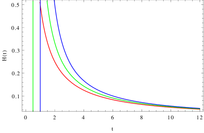
Using equations (11) and (45), the Hubble parameter is given by

H​(t)=1(2​tβˆ’c1)𝐻𝑑12𝑑subscript𝑐1\displaystyle H(t)=\frac{1}{(2t-c_{1})} (46)

where c1subscript𝑐1c_{1} is an integration constant.

Refer to caption
Figure 1: Plot for variation of the Hubble parameter H​(t)𝐻𝑑H(t) with cosmic time t𝑑t in radiation dominated phase. The red, green and blue curves correspond to c1=0,c1=1,c1=2formulae-sequencesubscript𝑐10formulae-sequencesubscript𝑐11subscript𝑐12c_{1}=0,c_{1}=1,c_{1}=2, respectively.

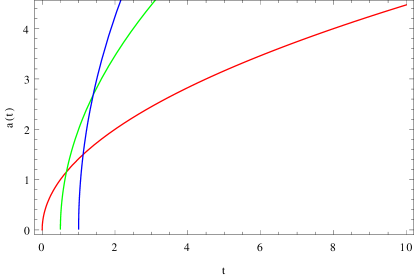
The scale factor for this era is given by

a​(t)=c2​(2​tβˆ’c1)12π‘Žπ‘‘subscript𝑐2superscript2𝑑subscript𝑐112\displaystyle a(t)=c_{2}(2t-c_{1})^{\frac{1}{2}} (47)

where c2subscript𝑐2c_{2} is another integration constant.

Refer to caption
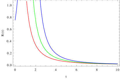
Figure 2: Plot for variation of the scale factor a​(t)π‘Žπ‘‘a(t) with cosmic time (0≀t≀100𝑑100\leq t\leq 10) in radiation dominated phase. The red, green and blue curves correspond to (c1,c2)≑(0,1);(c1,c2)≑(1,2);(c1,c2)≑(2,3)formulae-sequencesubscript𝑐1subscript𝑐201formulae-sequencesubscript𝑐1subscript𝑐212subscript𝑐1subscript𝑐223(c_{1},c_{2})\equiv(0,1);(c_{1},c_{2})\equiv(1,2);(c_{1},c_{2})\equiv(2,3), respectively.

In radiation dominated phase we confirm that the scale factor a​(t)∝t12proportional-toπ‘Žπ‘‘superscript𝑑12a(t)\propto t^{\frac{1}{2}}, which is same as in the case of standard model. Figures (1) and (2) show variation the Hubble parameter H​(t)𝐻𝑑H(t) and scale factor a​(t)π‘Žπ‘‘a(t) with time t𝑑t in radiation phase. As expected, the Ricci scalar R𝑅R for radiation dominated era is given by

R=0𝑅0\displaystyle R=0 (48)

VI Dynamics of matter dominated era

From the field equations (5)5(5) and (6)6(6) we obtain the following equation

βˆ’ΞΊ2​ρr3+3​F​H2+F​HΛ™βˆ’f2βˆ’2​H​FΛ™βˆ’FΒ¨=0superscriptπœ…2subscriptπœŒπ‘Ÿ33𝐹superscript𝐻2𝐹˙𝐻𝑓22𝐻˙𝐹¨𝐹0\displaystyle-\frac{\kappa^{2}\rho_{r}}{3}+3FH^{2}+F\dot{H}-\frac{f}{2}-2H\dot{F}-\ddot{F}=0 (49)

In phase space analysis of dynamical system, there is a point P5subscript𝑃5P_{5} which represents a standard matter era in the limit mβ†’0β†’π‘š0m\rightarrow 0. In matter dominated phase of the Universe

m​(q=βˆ’1)β‰ˆ0π‘šπ‘ž10\displaystyle m(q=-1)\approx 0 (50)

Using the definition of qπ‘žq or mπ‘šm, the form of f​(R)𝑓𝑅f(R) is given by

f​(R)=β​R𝑓𝑅𝛽𝑅\displaystyle f(R)=\beta R (51)

where β𝛽\beta is an integration constant. Thus, in matter dominated phase the form of f​(R)𝑓𝑅f(R) is similar as in the case of radiation dominated phase.

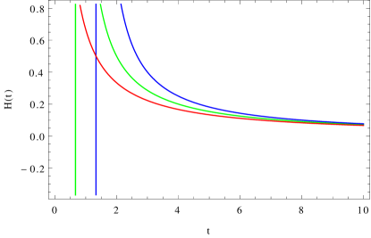
In matter dominated phase, we neglect the energy density of radiation i.e. ρr=0subscriptπœŒπ‘Ÿ0\rho_{r}=0. For f​(R)=β​R𝑓𝑅𝛽𝑅f(R)=\beta R, F=β𝐹𝛽F=\beta and therefore FΛ™=0˙𝐹0\dot{F}=0. Using equations (49) and (2) and these values of F𝐹F and F˙˙𝐹\dot{F}, the time evolution of the Hubble parameter is expressed as

H​(t)=1(32​tβˆ’c3)𝐻𝑑132𝑑subscript𝑐3\displaystyle H(t)=\frac{1}{(\frac{3}{2}t-c_{3})} (52)

where c3subscript𝑐3c_{3} is an integration constant.

Refer to caption
Figure 3: Plot for variation of the Hubble parameter H​(t)𝐻𝑑H(t) with cosmic time t𝑑t in matter dominated phase.The red, green and blue curves correspond to c3=0,c3=1,c3=2formulae-sequencesubscript𝑐30formulae-sequencesubscript𝑐31subscript𝑐32c_{3}=0,c_{3}=1,c_{3}=2, respectively.

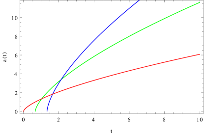
The scale factor in this phase is given by the expression

a​(t)=c4​(32​tβˆ’c3)23π‘Žπ‘‘subscript𝑐4superscript32𝑑subscript𝑐323\displaystyle a(t)=c_{4}\left(\frac{3}{2}t-c_{3}\right)^{\frac{2}{3}} (53)
Refer to caption
Figure 4: Plot for variation of the scale factor a​(t)π‘Žπ‘‘a(t) with cosmic time t𝑑t in matter dominated phase.The red, green and blue curves correspond to (c3,c4)≑(0,1);(c3,c4)≑(1,2);(c3,c4)≑(2,3)formulae-sequencesubscript𝑐3subscript𝑐401formulae-sequencesubscript𝑐3subscript𝑐412subscript𝑐3subscript𝑐423(c_{3},c_{4})\equiv(0,1);(c_{3},c_{4})\equiv(1,2);(c_{3},c_{4})\equiv(2,3), respectively.

From equations (2) and (52) the Ricci scalar in matter dominated phase is given by

R=3(32​tβˆ’c3)2𝑅3superscript32𝑑subscript𝑐32\displaystyle R=\frac{3}{(\frac{3}{2}t-c_{3})^{2}} (54)
Refer to caption
Figure 5: Plot for variation of Ricci scalar R𝑅R with cosmic time t𝑑t in matter dominated phase. The red, green and blue curves correspond to (c3,c4)≑(0,1);(c3,c4)≑(1,2);(c3,c4)≑(2,3)formulae-sequencesubscript𝑐3subscript𝑐401formulae-sequencesubscript𝑐3subscript𝑐412subscript𝑐3subscript𝑐423(c_{3},c_{4})\equiv(0,1);(c_{3},c_{4})\equiv(1,2);(c_{3},c_{4})\equiv(2,3), respectively.

The variation of Hubble parameter H​(t)𝐻𝑑H(t), scale factor a​(t)π‘Žπ‘‘a(t) and Ricci scalar R𝑅R, with time is plotted in figures (3), (4), and (5) respectively. Hubble parameterH​(t)𝐻𝑑H(t), scale factor a​(t)π‘Žπ‘‘a(t), and Ricci scalar R𝑅R in this phase can also be calculated by the same procedure as we followed in the radiation era. Expressions for these parameters are same in both approaches. For mβ‰ˆ0π‘š0m\approx 0, the effective equation of state is given by

we​f​f=0subscript𝑀𝑒𝑓𝑓0\displaystyle w_{eff}=0 (55)

These expressions of scale factor a​(t)π‘Žπ‘‘a(t), Hubble parameter H​(t)𝐻𝑑H(t), and Ricci scalar R𝑅R in matter dominated phase are similar to the expressions of standard (ΛΛ\LambdaCDM) model.

VII Dynamics of accelerated expansion dominated phase

In the phase space analysis, there is a point P1subscript𝑃1P_{1}, for which effective equation of state is

we​f​f=βˆ’1subscript𝑀𝑒𝑓𝑓1\displaystyle w_{eff}=-1 (56)

This point is called de Sitter point. If we take de Sitter expansion, this point is stable when 0<m<10π‘š10<m<1 at q=βˆ’2π‘ž2q=-2. Now from the definition of qπ‘žq, the form of f​(R)𝑓𝑅f(R) in this phase is given by

f​(R)=γ​R2𝑓𝑅𝛾superscript𝑅2\displaystyle f(R)=\gamma R^{2} (57)

We have the effective equation of state

we​f​f=βˆ’1βˆ’23​HΛ™H2subscript𝑀𝑒𝑓𝑓123˙𝐻superscript𝐻2\displaystyle w_{eff}=-1-\frac{2}{3}\frac{\dot{H}}{H^{2}} (58)

Now, using equations (56) and (58), in this phase we get the constant value of the Hubble parameter as

H​(t)=c5𝐻𝑑subscript𝑐5\displaystyle H(t)=c_{5} (59)

where c5subscript𝑐5c_{5} is an integration constant. Therefore, the Ricci scalar in this phase is given by

R=12​c52𝑅12superscriptsubscript𝑐52\displaystyle R=12c_{5}^{2} (60)

Using the expression of Hubble parameter H​(t)𝐻𝑑H(t), the scale factor is given by

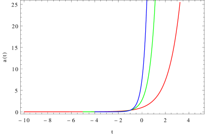
a​(t)=ec5​t+c6π‘Žπ‘‘superscript𝑒subscript𝑐5𝑑subscript𝑐6\displaystyle a(t)=e^{c_{5}t+c_{6}} (61)

where c6subscript𝑐6c_{6} is another integration constant. We can also find out these parameters using equations (49) and (2) in the spatially flat universe.
Refer to caption
Figure 6: Plot for variation of the scale factor a​(t)π‘Žπ‘‘a(t) with cosmic time t𝑑t in acceleration dominated phase. The red, green and blue curves correspond to (c5,c6)≑(1,0);(c5,c6)≑(2,1);(c5,c6)≑(3,2)formulae-sequencesubscript𝑐5subscript𝑐610formulae-sequencesubscript𝑐5subscript𝑐621subscript𝑐5subscript𝑐632(c_{5},c_{6})\equiv(1,0);(c_{5},c_{6})\equiv(2,1);(c_{5},c_{6})\equiv(3,2), respectively.

Here, figure (6) shows the variation of scale factor a​(t)π‘Žπ‘‘a(t) with time. It is clear that expansion in this phase is exponential. This behaviour is found to be similar to the case of the standard (ΛΛ\LambdaCDM) model.

VIII Asymmetry of time

We rewrite the action (3) in the form

π’œ=βˆ«βˆ’g​(12​κ2​F​Rβˆ’U)​d4​x+π’œm,π’œπ‘”12superscriptπœ…2πΉπ‘…π‘ˆsuperscript𝑑4π‘₯subscriptπ’œπ‘š\displaystyle\mathcal{A}=\int\sqrt{-g}\left(\frac{1}{2\kappa^{2}}FR-U\right)d^{4}x+\mathcal{A}_{m}, (62)

where

U=F​Rβˆ’f2​κ2.π‘ˆπΉπ‘…π‘“2superscriptπœ…2\displaystyle U=\frac{FR-f}{2\kappa^{2}}. (63)

It is possible to derive an action in the Einstein frame under the conformal transformation

g~μ​ν=Ξ©2​gμ​ν,subscript~π‘”πœ‡πœˆsuperscriptΞ©2subscriptπ‘”πœ‡πœˆ\displaystyle\tilde{g}_{\mu\nu}=\Omega^{2}g_{\mu\nu}, (64)

where Ξ©2superscriptΞ©2\Omega^{2} is the conformal factor and a tilde denotes the quantities pertaining to the Einstein frame. The corresponding Ricci scalars in the two frames are related as

R=Ξ©2​(R~+6​░~β€‹Ο‰βˆ’6​g~ΞΌβ€‹Ξ½β€‹βˆ‚ΞΌΟ‰β€‹βˆ‚Ξ½Ο‰),𝑅superscriptΞ©2~𝑅6~β–‘πœ”6superscript~π‘”πœ‡πœˆsubscriptπœ‡πœ”subscriptπœˆπœ”\displaystyle R=\Omega^{2}(\tilde{R}+6\tilde{\Box}\omega-6\tilde{g}^{\mu\nu}\partial_{\mu}\omega\partial_{\nu}\omega), (65)

where

ω≑ln⁑Ω,βˆ‚ΞΌΟ‰β‰‘βˆ‚Ο‰βˆ‚x~ΞΌ,β–‘~​ω≑1βˆ’g~β€‹βˆ‚ΞΌ(βˆ’g~​g~ΞΌβ€‹Ξ½β€‹βˆ‚Ξ½Ο‰).formulae-sequenceπœ”Ξ©formulae-sequencesubscriptπœ‡πœ”πœ”superscript~π‘₯πœ‡~β–‘πœ”1~𝑔subscriptπœ‡~𝑔superscript~π‘”πœ‡πœˆsubscriptπœˆπœ”\displaystyle\omega\equiv\ln\Omega,\partial_{\mu}\omega\equiv\frac{\partial\omega}{\partial\tilde{x}^{\mu}},\tilde{\Box}\omega\equiv\frac{1}{\sqrt{-\tilde{g}}}\partial_{\mu}(\sqrt{-\tilde{g}}\tilde{g}^{\mu\nu}\partial_{\nu}\omega). (66)

Thus, the action (62) is transformed as

π’œ=∫d4​xβ€‹βˆ’g~​[12​κ2​Fβ€‹Ξ©βˆ’2​(R~+6​░~β€‹Ο‰βˆ’6​g~ΞΌβ€‹Ξ½β€‹βˆ‚ΞΌΟ‰β€‹βˆ‚Ξ½Ο‰)βˆ’Ξ©βˆ’4​U]π’œsuperscript𝑑4π‘₯~𝑔delimited-[]12superscriptπœ…2𝐹superscriptΞ©2~𝑅6~β–‘πœ”6superscript~π‘”πœ‡πœˆsubscriptπœ‡πœ”subscriptπœˆπœ”superscriptΞ©4π‘ˆ\displaystyle\mathcal{A}=\int d^{4}x\sqrt{-\tilde{g}}\left[\frac{1}{2\kappa^{2}}F\Omega^{-2}(\tilde{R}+6\tilde{\Box}\omega-6\tilde{g}^{\mu\nu}\partial_{\mu}\omega\partial_{\nu}\omega)-\Omega^{-4}U\right]
+π’œm.subscriptπ’œπ‘š\displaystyle+\mathcal{A}_{m}.
(67)

The linear action in R~~𝑅\tilde{R} can be written by choosing

Ω2=F.superscriptΩ2𝐹\displaystyle\Omega^{2}=F. (68)

We consider a new scalar field Ο•italic-Ο•\phi defined by

κ​ϕ≑32​ln⁑F.πœ…italic-Ο•32𝐹\displaystyle\kappa\phi\equiv\sqrt{\frac{3}{2}}\ln F. (69)

Using these relations the action in Einstein frame is found as a15

π’œ=∫d4​xβ€‹βˆ’g~​[12​κ2​R~βˆ’12​g~ΞΌβ€‹Ξ½β€‹βˆ‚ΞΌΟ•β€‹βˆ‚Ξ½Ο•βˆ’V​(Ο•)]+π’œm.π’œsuperscript𝑑4π‘₯~𝑔delimited-[]12superscriptπœ…2~𝑅12superscript~π‘”πœ‡πœˆsubscriptπœ‡italic-Ο•subscript𝜈italic-ϕ𝑉italic-Ο•subscriptπ’œπ‘š\displaystyle\mathcal{A}=\int d^{4}x\sqrt{-\tilde{g}}\left[\frac{1}{2\kappa^{2}}\tilde{R}-\frac{1}{2}\tilde{g}^{\mu\nu}\partial_{\mu}\phi\partial_{\nu}\phi-V(\phi)\right]+\mathcal{A}_{m}.
(70)

where

V​(Ο•)=UF2=F​Rβˆ’f2​κ2​F2.𝑉italic-Ο•π‘ˆsuperscript𝐹2𝐹𝑅𝑓2superscriptπœ…2superscript𝐹2\displaystyle V(\phi)=\frac{U}{F^{2}}=\frac{FR-f}{2\kappa^{2}F^{2}}. (71)

On varying the action (70) w.r.t. Ο•italic-Ο•\phi in the absence of matter (relativistic and non-relativistic, both), we get

d2​ϕd​t~2+3​H~​d​ϕd​t~+V,Ο•=0.\displaystyle\frac{d^{2}\phi}{d\tilde{t}^{2}}+3\tilde{H}\frac{d\phi}{d\tilde{t}}+V_{,\phi}=0. (72)

with V,Ο•V_{,\phi} implying the usual derivative w.r.t. Ο•italic-Ο•\phi. The energy density and pressure of the above homogeneous scalar field, respectively, are

ρ=12​ϕ˙2+V​(Ο•);p=12​ϕ˙2βˆ’V​(Ο•),formulae-sequence𝜌12superscriptΛ™italic-Ο•2𝑉italic-ϕ𝑝12superscriptΛ™italic-Ο•2𝑉italic-Ο•\displaystyle\rho=\frac{1}{2}\dot{\phi}^{2}+V(\phi);p=\frac{1}{2}\dot{\phi}^{2}-V(\phi), (73)

while the scalar field equation of motion is given by (72).

Tolman described a cyclic universe with progressively larger cycles, assuming the presence of a viscous fluid with pressure

p=p0βˆ’3​΢​H,𝑝subscript𝑝03𝜁𝐻\displaystyle p=p_{0}-3\zeta H, (74)

where p0subscript𝑝0p_{0} is the equilibrium pressure and ΢𝜁\zeta is the coefficient of bulk viscositya14 . It is clear from equation (74) that p<p0𝑝subscript𝑝0p<p_{0} during expansion (H>0)𝐻0(H>0) whereas p>p0𝑝subscript𝑝0p>p_{0} during contraction. This asymmetry during the expanding and contracting phases results in the growth of both energy and entropy. This increase in entropy makes the amplitude of successive expansion cycles larger leading to a arrow of time.

In our discussion of f​(R)𝑓𝑅f(R) gravity models, the term 3​H~​d​ϕd​t~3~𝐻𝑑italic-ϕ𝑑~𝑑3\tilde{H}\frac{d\phi}{d\tilde{t}} in (72) behaves like friction and damps the motion of the scalar field when the universe (H>0)𝐻0(H>0). In a contracting universe, however, this term behaves like anti-friction and accelerates the motion of the scalar field. A scalar field with the potential V=M2​ϕ2𝑉superscript𝑀2superscriptitalic-Ο•2V=M^{2}\phi^{2} gives pβ‰ƒβˆ’Οsimilar-to-or-equalsπ‘πœŒp\simeq-\rho when H>0𝐻0H>0 and p≃ρsimilar-to-or-equalsπ‘πœŒp\simeq\rho when H<0𝐻0H<0. These results are in conformity with those of Tolman.

Further, we derive different potentials in all the phases of the Universe. In radiation dominated phase we have f​(R)=α​R,𝑓𝑅𝛼𝑅f(R)=\alpha R, therefore, the potential given by equation (71)is V​(Ο•)=0𝑉italic-Ο•0V(\phi)=0 for this phase. Similarly, for matter dominated phase we have f​(R)=β​R𝑓𝑅𝛽𝑅f(R)=\beta R and V​(Ο•)=0𝑉italic-Ο•0V(\phi)=0. For accelerated expansion phase, the form of the Lagrangian is given by including f​(R)=γ​R2𝑓𝑅𝛾superscript𝑅2f(R)=\gamma R^{2} and the potential for this phase is V​(Ο•)=18​γ​κ2𝑉italic-Ο•18𝛾superscriptπœ…2V(\phi)=\frac{1}{8\gamma\kappa^{2}}.

The scalar field given by equation (69) gives κ​ϕ=32​lnβ‘Ξ±πœ…italic-Ο•32𝛼\kappa\phi=\sqrt{\frac{3}{2}}\ln\alpha for matter dominated phase and κ​ϕ=32​lnβ‘Ξ²πœ…italic-Ο•32𝛽\kappa\phi=\sqrt{\frac{3}{2}}\ln\beta for radiation dominated phase. For accelerated expansion phase

κ​ϕ=32​ln⁑(2​γ​R)πœ…italic-Ο•322𝛾𝑅\displaystyle\kappa\phi=\sqrt{\frac{3}{2}}\ln(2\gamma R) (75)

The general solution of the equation (72) for the potential V​(Ο•)=12​M2​ϕ2𝑉italic-Ο•12superscript𝑀2superscriptitalic-Ο•2V(\phi)=\frac{1}{2}M^{2}\phi^{2} is given by

Ο•=Ο•02​exp⁑(βˆ’Ξ¨β€‹t)​(1+ΨΨ2βˆ’M2)​exp⁑(Ξ¨2βˆ’M2)​t+italic-Ο•limit-fromsubscriptitalic-Ο•02Ψ𝑑1Ξ¨superscriptΞ¨2superscript𝑀2superscriptΞ¨2superscript𝑀2𝑑\displaystyle\phi=\frac{\phi_{0}}{2}\exp(-\Psi t)\left(1+\frac{\Psi}{\sqrt{\Psi^{2}-M^{2}}}\right)\exp(\sqrt{\Psi^{2}-M^{2}})t+
Ο•02​exp⁑(βˆ’Ξ¨β€‹t)​(1βˆ’Ξ¨Ξ¨2βˆ’M2)​exp⁑(βˆ’Ξ¨2βˆ’M2)​tsubscriptitalic-Ο•02Ψ𝑑1Ξ¨superscriptΞ¨2superscript𝑀2superscriptΞ¨2superscript𝑀2𝑑\displaystyle\frac{\phi_{0}}{2}\exp(-\Psi t)\left(1-\frac{\Psi}{\sqrt{\Psi^{2}-M^{2}}}\right)\exp(-\sqrt{\Psi^{2}-M^{2}})t
(76)

where Ο•0subscriptitalic-Ο•0\phi_{0} is the maximum value of scalar field Ο•italic-Ο•\phi at t=0𝑑0t=0 (t𝑑t being the time in the Einstein frame henceforth), Ξ¨=3​H~2Ξ¨3~𝐻2\Psi=\frac{3\tilde{H}}{2}, and M𝑀M is the mass of the scalar field. In this solution three cases arises depending on the value of Ξ¨2βˆ’M2superscriptΞ¨2superscript𝑀2\sqrt{\Psi^{2}-M^{2}} as discussed below.

VIII.1 Case (i): M2>Ξ¨2superscript𝑀2superscriptΞ¨2M^{2}>\Psi^{2}

In this case the solution is given by

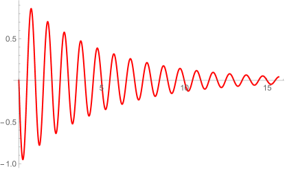
Ο•=Ο•0​Mω​exp⁑(βˆ’Ξ¨β€‹t)​sin⁑(ω​t+ΞΈ)italic-Ο•subscriptitalic-Ο•0π‘€πœ”Ξ¨π‘‘πœ”π‘‘πœƒ\displaystyle\phi=\frac{\phi_{0}M}{\omega}\exp(-\Psi t)\sin(\omega t+\theta) (77)

where Ο‰=M2βˆ’Ξ¨2πœ”superscript𝑀2superscriptΞ¨2\omega=\sqrt{M^{2}-\Psi^{2}} and ΞΈπœƒ\theta is the phase angle. If we take ΨΨ\Psi as a positive constant, then figure (7) shows the nature of scalar field in this case. These oscillations are damped harmonic oscillations. In the perturbations due to local gravity, a very large field mass corresponds to smaller deviations from the standard ΛΛ\LambdaCDM model.

Refer to caption
Figure 7: Plot for variation of scalar field Ο•italic-Ο•\phi along Yβˆ’limit-fromπ‘ŒY-axis with time t𝑑t along Xβˆ’limit-from𝑋X-axis in case M2>Ξ¨2superscript𝑀2superscriptΞ¨2M^{2}>\Psi^{2} . Here, we have taken Ξ¨=15Ξ¨15\Psi=\frac{1}{5}, Ο•0​MΟ‰=1subscriptitalic-Ο•0π‘€πœ”1\frac{\phi_{0}M}{\omega}=1, Ο‰=2β€‹Ο€πœ”2πœ‹\omega=2\pi and ΞΈ=Ο€πœƒπœ‹\theta=\pi.

VIII.2 Case (ii): M2<Ξ¨2superscript𝑀2superscriptΞ¨2M^{2}<\Psi^{2}

The general solution of field equation is given by

Ο•=Ο•02​exp⁑(βˆ’Ξ¨β€‹t)​(1+ΨΨ2βˆ’M2)​exp⁑(Ξ¨2βˆ’M2)​t+italic-Ο•limit-fromsubscriptitalic-Ο•02Ψ𝑑1Ξ¨superscriptΞ¨2superscript𝑀2superscriptΞ¨2superscript𝑀2𝑑\displaystyle\phi=\frac{\phi_{0}}{2}\exp(-\Psi t)\left(1+\frac{\Psi}{\sqrt{\Psi^{2}-M^{2}}}\right)\exp(\sqrt{\Psi^{2}-M^{2}})t+
Ο•02​exp⁑(βˆ’Ξ¨β€‹t)​(1βˆ’Ξ¨Ξ¨2βˆ’M2)​exp⁑(βˆ’Ξ¨2βˆ’M2)​tsubscriptitalic-Ο•02Ψ𝑑1Ξ¨superscriptΞ¨2superscript𝑀2superscriptΞ¨2superscript𝑀2𝑑\displaystyle\frac{\phi_{0}}{2}\exp(-\Psi t)\left(1-\frac{\Psi}{\sqrt{\Psi^{2}-M^{2}}}\right)\exp(-\sqrt{\Psi^{2}-M^{2}})t
(78)

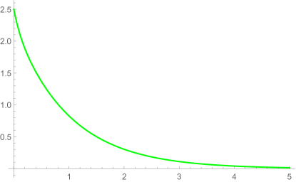
In this case (Ξ¨2βˆ’M2)superscriptΞ¨2superscript𝑀2(\Psi^{2}-M^{2}) is a positive quantity and there is an exponential term with negative power. So, the field dies off exponentially with time. There is no oscillation and the motion become over-damped. Figure (8) shows the behaviour of the scalar field Ο•italic-Ο•\phi with time t𝑑t.

Refer to caption
Figure 8: Plot for variation of the scalar field Ο•italic-Ο•\phi along Yβˆ’limit-fromπ‘ŒY-axis with time t𝑑t along Xβˆ’limit-from𝑋X-axis in case M2<Ξ¨2superscript𝑀2superscriptΞ¨2M^{2}<\Psi^{2}. The values of the parameters are as Ξ¨=5Ξ¨5\Psi=5, M=3𝑀3M=3, and Ο•0=2subscriptitalic-Ο•02\phi_{0}=2.

VIII.3 Case (iii): M2=Ξ¨2superscript𝑀2superscriptΞ¨2M^{2}=\Psi^{2}

This is a special case, appearing as the critical damping of the scalar field. The solution is given as

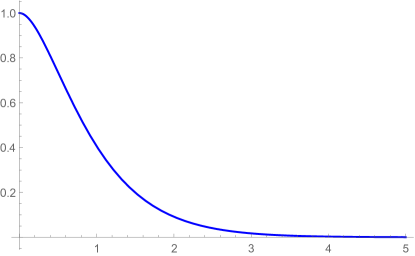
Ο•=Ο•0​exp⁑(βˆ’Ξ¨β€‹t)​(1+Ψ​t)italic-Ο•subscriptitalic-Ο•0Ψ𝑑1Ψ𝑑\displaystyle\phi=\phi_{0}\exp(-\Psi t)(1+\Psi t) (79)

indicating an aperiodic damping. Figure (9) shows the nature of the scalar field Ο•italic-Ο•\phi with the positive ΨΨ\Psi.

Refer to caption
Figure 9: Plot for variation of scalar field Ο•italic-Ο•\phi along Yβˆ’limit-fromπ‘ŒY-axis with time t𝑑t along Xβˆ’limit-from𝑋X-axis in case M2=Ξ¨2superscript𝑀2superscriptΞ¨2M^{2}=\Psi^{2}. Here, we have taken Ξ¨=2Ξ¨2\Psi=2 and Ο•0=1subscriptitalic-Ο•01\phi_{0}=1.

It is clear that in all the above cases we get a damping either periodic or aperiodic that owes its relation to Ξ¨=3​H~2Ξ¨3~𝐻2\Psi=\frac{3\tilde{H}}{2} and mass M𝑀M of the scalar field Ο•italic-Ο•\phi. When H~~𝐻\tilde{H} is positive and constant, ΨΨ\Psi damps the scalar field. When ΨΨ\Psi is negative and constant, the motion of the scalar field accelerates in all the three cases.

We also find that the scalar field is not symmetric under the reversal of time i.e. (tβ†”βˆ’t)↔𝑑𝑑(t\leftrightarrow-t) for positive and negative Ξ¨=3​H~2Ξ¨3~𝐻2\Psi=\frac{3\tilde{H}}{2}. This dissipation of the scalar field indicates a crucial asymmetry in time in form of its arrow from past to future.

IX Conclusion

While describing the f​(R)𝑓𝑅f(R) models of modified gravity, we have studied the properties and stability of the fixed points of the dynamical system against the time dependent perturbations in a smooth spatial background. We discussed the role of radiation in our analysis and compared it with the case without radiation. It is found that the nature of the fixed points with radiation remains unaltered as that without radiation (except that with radiation we have the emergence of an extra eigenvalue for each point). (Of course, the future discussion would bring out an analysis of the fixed points against spatial perturbations as well). We have determined the forms of f​(R)𝑓𝑅f(R) for different phases of the universe, over radiation, matter and acceleration dominated eras, by using the necessary conditions for the phase space analysis to reach eventually at a cosmologically viable model. The scale factor a​(t)π‘Žπ‘‘a(t), the Hubble parameter H​(t)𝐻𝑑H(t), Ricci scalar R𝑅R have been determined for these phases, with a view that their ordering over the entire evolution of the universe may explain the emergence of an arrow of time, more comprehensively in a future study. While these model parameters are found to be consistent with ΛΛ\LambdaCDM model, the crucial issue is that the scalar field Ο•italic-Ο•\phi, that owes its origin exclusively to f​(R)𝑓𝑅f(R) gravity, may be invoked to explain the arrow of time based on its explicit asymmetry on a classical level. While the scalar-tensor theories may have the forms of potentials matching with f​(R)𝑓𝑅f(R), the results obtained on the stability conditions and their ordering extending through the overall history may not be reproduced in such theories. We would further explore this fundamental aspect of the nature of time and its observational viability within the modified gravity sector.

Acknowledgements.
MMV thanks Edward Kolb at the Kavli Institute of Cosmological Physics, the University of Chicago, USA for hosting the visit, and Varun Sahni at the Inter-University Centre for Astronomy and Astrophysics (IUCAA), Pune, India for discussion and facilities. Both authors thank IUCAA for the support under the associateship programme.

References

  • (1) A. G. Riess et al., (Supernova Search Team Collaboration), Astron. J. 116, 1009 (1998).
  • (2) B. Schmidt et al., Astrophys. J. 507, 46 (1998).
  • (3) S. Perlmutter et al., Astrophys. J. 517, 565 (1999).
  • (4) D. N. Spergel et al., Astrophys. J. Suppl. 148, 97 (2003).
  • (5) T. Padmanabhan, Phys. Rept., textbf380, 235 (2003).
  • (6) R. R. Caldwell, R. Dave, and P. J. Steinhardt, Phys. Rev. Lett. 80, 1582 (1998).
  • (7) S. Capozziello, Int. J. Mod. Phys. D 11, 483 (2002)
  • (8) T. Chiba, T. Okabe, and M. Yamaguchi, Phys. Rev. D 62, 023511 (2000).
  • (9) R. R. Caldwell, Phys. Lett. B 545, 23 (2002).
  • (10) A. A. Starobinski, Phys. Lett. B 91, 99(1980).
  • (11) M. Kunz and D. Sapone, Phys. Rev. Lett. 98, 121301 (2007).
  • (12) L. Amendola, R. Gannouji, D. Polarski and S. Tsujikawa, Phys. Rev. D 75, 083504 (2007).
  • (13) V. Sahni and Y. Shantov, JCAP 0311, 014 (2003).
  • (14) R. C. Tolman, Relativity, Thermodynamics and Cosmology (Oxford: Clarendon) (1934).
  • (15) L. Amendola and S. Tsujikawa, Dark energy: Theory and Observations (Cambridge) (2010).