Drag induced radiative loss from semi-hard heavy quarks

Abstract

The case of gluon bremsstrahlung off a heavy quark in extended nuclear matter is revisited within the higher twist formalism. In particular, the in-medium modification of “semi-hard” heavy quarks is studied, where the momentum of the heavy quark is larger but comparable to the mass of the heavy quark ($p\gtrsim M$). In contrast to all prior calculations, where the gluon emission spectrum is entirely controlled by the transverse momentum diffusion parameter ($\hat{q}$), both for light and heavy quarks, in this work, we demonstrate that the gluon emission spectrum for a heavy quark (unlike that for flavors) is also sensitive to $\hat{e}$, which so far has been used to quantify the amount of light-cone drag experienced by a parton. This mass dependent effect, due to the non-light-like momentum of a semi-hard heavy-quark, leads to an additional energy loss term for heavy-quarks, while resulting in a negligible modification of light flavor (and high energy heavy flavor) loss. This result can be used to estimate the value of this sub-leading non-perturbative jet transport parameter ($\hat{e}$) from heavy flavor suppression in ultra-relativistic heavy-ion collisions.

I Introduction

The unprecedented centre of mass energies available at the Large Hadron Collider have opened new windows for the exploration of extreme nuclear matter through high energy jets Wang:1991xy ; Gyulassy:1993hr ; Baier:1996kr ; Zakharov:1996fv ; Majumder:2010qh ; Wiedemann:2009sh . While a large portion of the available data on leading (and next-to-leading) particle suppression in the light flavor sector has been theoretically described using factorized pQCD based calculations of jet modification Armesto:2011ht ; Qin:2009gw , heavy quarks have remained somewhat of a challenge Djordjevic:2013pba . This is especially true in the semi-hard sector, where the momentum of the heavy quark is larger but comparable to its mass $p\gtrsim m_{Q}$. We distinguish this region from that of slow heavy quarks, where $p\lesssim m_{Q}$, which appear to be thermalized with the bulk medium, and fast heavy-quarks, with $p\gg m_{Q}$ which engender energy loss and suppression similar to light quarks.

The so called “heavy-quark puzzle” had already begun to manifest itself in measurements of the suppression of high transverse momentum (high-$p_{T}$) non-photonic electrons at the Relativistic Heavy-Ion Collider (RHIC). Measurements by both the STAR Abelev:2006db and PHENIX Adare:2006nq detectors showed a slightly higher suppression than expected, based on a calculation that included both drag and radiative loss Qin:2009gw ; Djordjevic:2003zk ; Djordjevic:2004nq . This trend has continued at the Large Hadron Collider (LHC) where the ALICE experiment has measured $D$ and $B$ meson suppression separately, and finds a larger than expected suppression in the semi-hard regime of heavy-quark momentum (we note that the case is not very clear for B-meson suppression which has so far only been presented as $p_{T}$ integrated points)ALICE:2012ab ; Aamodt:2010jd .

A considerable amount of theoretical work has been devoted to understand this larger than expected suppression of single electrons or heavy mesons arising from the fragmentation of a heavy-quark. However, most of these may be understood as falling in two categories: Calculations that have extended the base formalism of radiated energy loss for light flavors to include mass dependent terms, as well as a drag term to include the prominent role played by drag in heavy flavor energy loss   Zhang:2004qm ; Qin:2009gw ; Mustafa:2004dr ; Abir:2011jb ; Abir:2012pu ; Wicks:2005gt . Calculations that have ignored the role of radiative loss and only focussed on drag loss He:2012xz ; Cao:2011et ; Moore:2004tg .

In all calculations above, radiative loss is stimulated by transverse momentum diffusion experienced by the heavy quark or radiated gluon, which, in some cases, is quantified by the jet transport coefficient $\hat{q}$ Baier:2002tc ; Majumder:2012sh . The drag loss is quantified using the drag coefficient referred to as $dE/dx$ (energy loss per unit distance) or $\hat{e}$ Majumder:2008zg .

To the best of our knowledge, no calculation of heavy flavor energy loss has explored the possibility that the drag coefficient $\hat{e}$ (or the longitudinal diffusion coefficient $\hat{e}_{2}$) may lead to an additional source of radiative loss, beyond that provided by $\hat{q}$. This possibility is immediately clear in the higher twist framework, where the drag (and longitudinal diffusion) coefficient $\hat{e}$ ($\hat{e}_{2}$) has the boost invariant definition as the loss of light-cone momentum (fluctuation in light-cone momentum) per unit light-cone length, (assuming a parton moving in the negative light-cone direction)

$$\hat{e}=\frac{d\langle\Delta p^{-}\rangle}{dL^{-}},\,\,\,\,\,\,\,\,\,\,\hat{e}_{2}=\frac{d\langle\Delta{p^{-}}^{2}\rangle}{dL^{-}}.$$ (1)

While such a transport coefficient leads to little change in the off-shellness of a near on-shell massless quark, it has a considerable impact on the off-shellness of a near on-shell massive quark. No doubt, such a term will only have an effect on the radiative loss of a patron where the momentum $p$ is comparable to the mass $M$, thus for light flavors, and for energetic heavy-quarks where, $p\gg M$, this term will have a minimal effect. This was explicitly explored for photon radiation from a light quark in Ref. Qin:2014mya . We point out that such an effect is by no means limited to the higher-twist scheme, but effects several other formalisms that have considered the radiative loss from a heavy-quark in a quark gluon plasma.

In this paper, we will explore the modification to the calculation of radiative loss, due to the presence of this additional source within the higher twist formalism. To delineate the importance of these terms, we will use power-counting techniques borrowed from Soft-Collinear-Effective-Theory (SCET) Bauer:2000yr ; Bauer:2001ct ; Bauer:2002nz ; Bauer:2001yt to identify the regime where these mass dependent terms will cause detectable effects on the gluon bremsstrahlung spectrum. As a first attempt, we will consider only the case of single scattering and single emission. Arguments presented in subsequent sections will demonstrate this to be the leading contribution, given the short formation time of the radiated gluons. In this paper, the analytical expressions for the $\hat{e}$ ($\hat{q}$ and $\hat{e}_{2}$) induced gluon radiation spectrum will be derived. Numerical calculations for the suppression of $B$ and $D$ mesons, as well as the suppression and azimuthal anisotropy of non-photonic leptons from the decay of these mesons at LHC and RHIC energies, and comparisons with experimental data will be carried out in a subsequent effort.

The article is organized as follows: in Sec. II, we will setup the basic formalism of Deep Inelastic Scattering (DIS) on a large nucleus, where the hard virtual photon strikes a heavy-quark, assumed to be produced in a rare high $Q^{2}$ fluctuation inside a proton. In Sec. III, we will carry out diagrammatic studies on the induced gluon radiation off the heavy quark in this system, within the higher twist formalism. We will present and discuss final expressions for gluon bremsstrahlung from such a heavy quark, containing both $\hat{q}$, $\hat{e}$ and $\hat{e}_{2}$ in Sec. IV. We offer concluding discussions and an outlook in Sec. V. Involved expressions for a set of diagrams are contained in the appendix.

II Deep inelastic scattering and the semi-hard heavy quark

The set-up is based on the deep-inelastic scattering of a virtual photon off a heavy quark within a large nucleus with mass number $A$. We will study the case where the hard virtual photon scatters with the hard heavy quark converting it to slow moving heavy quark (this is defined below). The propagation of the heavy-quark will be factorized from the hard scattering vertex which produces the outgoing slow moving heavy-quark. The nucleus has a momentum $P=pA$, where $p$ is the average momentum of a nucleon in this nucleus. In the Breit frame, the exchanged virtual photon possesses no transverse momentum,

$$q\equiv[q^{+},q^{-},q_{\perp}]=\left[q^{+},q^{-},0\right].$$ (2)

The process under consideration is the following:

$$e(L_{1})+A(P)\rightarrow e(L_{2})+J_{\cal Q}(L_{\cal Q})+X.$$ (3)

In the above process, $e(L_{1})$ and $e(L_{2})$ represent the incoming (outgoing) electron with momentum $L_{1}$ and $L_{2}$ respectively. The factor $A(P)$ represents the incoming nucleus with momentum $P$. The factor $J_{\cal Q}(L_{\cal Q})$ is the outgoing jet which contains one heavy quark $\cal Q$. In the particular diagrams that we will consider, the final strongly interacting particles Due to the absence of valence heavy-quarks within the nucleon, the photon will have to strike a heavy quark from s ${\cal Q}\bar{\cal Q}$ fluctuation within the sea of partons. Alternatively one may consider the case of a $J/\psi$ or $\Upsilon$ state bound within a large nucleus, being struck by the hard virtual photon. More detail discussions on the production of heavy quark can be found in Abir:2014sxa . In this work, we will not discuss the production of the heavy quark further. For the purposes of this calculation, this is now contained within a parton distribution function. In essence, by this mechanism a semi-hard heavy quark has been produced. In what follows, we will focus on the power counting of the momentum components and the modification of the final state.

Similar to Ref Abir:2014sxa , we will consider a quark mass $M\gg\Lambda_{QCD}$ and a final outgoing quark momentum which is larger, but of the order of the quark mass. We assume that the quark, anti-quark fluctuations possess minimal momentum in the rest frame of the nucleus, and thus its momentum components scales as $\left(p_{\cal Q}^{+},p_{\cal Q}^{-},p_{\cal Q\perp}\right)\sim\left(M/\sqrt{2},~{}M/\sqrt{2},~{}0\right)$. Now in a frame where the nucleus is boosted by a large boost factor $\gamma$ in the $``+\textquotedblright$ direction, momentum components of the incoming heavy quark will scales as,

$$p_{\cal Q}=\left[p_{\cal Q}^{+},p_{\cal Q}^{-},p_{\cal Q\perp}\right]\equiv\left[\gamma\frac{M}{\sqrt{2}},~{}\frac{1}{\gamma}\frac{M}{\sqrt{2}},~{}0\right].$$ (4)

It is important to note that the boost factor $\gamma$ carries no extra information other than the the fact that $p_{\cal Q}^{+}$ is very large compare to $p_{\cal Q}^{-}$. We assume the momentum components of the incoming photon to be,

$$q=\left[-\gamma\frac{M}{\sqrt{2}}+\frac{M^{2}}{2q^{-}},~{}q^{-}-\frac{1}{\gamma}\frac{M}{\sqrt{2}},~{}0\right].$$ (5)

Given a large boost factor $(\gamma)$, one can assume that $\gamma M\gg M\sim q^{-}\gg M/\gamma$. Hence, we define the hard scale $Q$ as $Q^{2}=-q^{2}\simeq\gamma Mq^{-}/\sqrt{2}$. As a result, we obtain the final out-going quark to have momentum components as,

$$p_{f}=p_{\cal Q}+q=\left[\frac{M^{2}}{2q^{-}},q^{-},0\right].$$ (6)

We consider $M\lesssim q^{-}\sim\sqrt{\lambda}Q$ where $\lambda\sim 1/\gamma$ for this “semi-hard” heavy quark. The term “semi-hard” defines a quark whose momentum is not an order of magnitude larger than its mass.

II.1 Power Counting and the small $\lambda$ parameter

In order to set up the power counting, in this study, we have introduced the dimensionless small parameter $\lambda$. Power corrections to hard process are generally suppressed by factors of a hard scale, $Q^{2}\gg\Lambda_{QCD}$. The introduction of the parameter $\lambda$ to represent semi-hard scales as $\lambda Q$ and softer scales as $\lambda^{2}Q$, is a concept borrowed from soft collinear effective theory (SCET)  Idilbi:2008vm ; D'Eramo:2010ak . In what follows, we will retain leading and next-to-leading terms in $\lambda$ power counting, neglecting all terms which scale with $\lambda^{2}$ or a higher power of $\lambda$ Qin:2012fua . We have chosen the scaling variable $\lambda$ in such a way that perturbation theory may be applied down to momentum transfer scales at or above $\lambda^{3/2}Q\sim\Lambda_{\rm QCD}$. In our study,

$$\lambda^{0}\gg\sqrt{\lambda}\gg\lambda\gg{\lambda}^{\frac{3}{2}}.$$ (7)

Based on the power counting set up and the choice of incoming and outgoing quark momentum, we can outline several important scales in the problem of a heavy quark propagating through the nuclear medium, scattering off constituents in the medium and emitting real gluons. We remind the reader that given the semi-hard momentum of the heavy quark, collinear emission is suppressed due to the mass of the heavy quark, i.e., the dead cone effect Dokshitzer:2001zm . In the subsequent section, the calculation of the process of single scattering and single emission from a heavy quark will be carried out. Here we outline the power counting (in $\lambda$) of the relevant momentum components that will arise in the calculation. The virtuality of the hard photon defines the hardest scale in the problem, $Q$, similar to the case of light quark production in DIS. The incoming or initial heavy quark has momentum components $p_{i}\sim(\lambda^{-\frac{1}{2}},\lambda^{\frac{3}{2}},0)Q$, the outgoing heavy quark has momentum components $p\sim(\sqrt{\lambda},\sqrt{\lambda},0)Q$. The mass of the semi-hard heavy quark scales as $M\sim\sqrt{\lambda}Q$. This choice of incoming parton and photon momenta ensures that the momentum of the final outgoing heavy quark is of the order of its momentum. In what follows, we will demonstrate that the leading contribution to gluon emission arises from the region where real emitted gluons have momenta which scale as $l\sim(\lambda,\lambda,\lambda)Q$. The fraction of light cone momenta carried out by the gluon is $y=l^{-}/p^{-}\sim\sqrt{\lambda}$. Also somewhat different from the case of light flavors is the scaling of the virtual Glauber gluons : $k\sim(\lambda^{\frac{3}{2}},\lambda^{\frac{3}{2}},\lambda)Q$ with $k^{2}=2k^{+}k^{-}-k_{\perp}^{2}\simeq-k_{\perp}^{2}$. As we will demonstrate below, these choices of momentum scales tend to enhance the gluon emission rate.

There is another consequence of this choice of scales which relates to how the single gluon emission kernel may be iterated. Unlike the case for light flavors, the formation length of a gluon with momentum components $l\sim(\lambda,\lambda,\lambda)Q$ is

$$\tau_{Q}=\frac{2l^{-}}{l_{\perp}^{2}}\sim\frac{1}{\lambda Q},$$ (8)

is rather short compared to the formation length of $\tau_{q}\sim~{}1/\lambda^{2}Q$ for gluon radiation from near on-shell light flavors. This indicates that there cannot be many scatterings per emission. As a result, in what follows, we derive the single scattering per gluon emission rate. This single gluon emission kernel, induced by single scattering will have to be iterated to obtain the full energy loss of a semi-hard quark.

Many readers may find the presence of factors of $\sqrt{\lambda}$ somewhat disconcerting. We could have simply replaced this with a new $\lambda$. We refrain from defining a new dimensionless parameter $\lambda$, so as to make contact with prior definitions of $\lambda$ used in the case of light quarks, where $\lambda Q$ represented the transverse momentum of the radiated gluons from a hard parton, or the transverse momentum from scattering of a gluon in the medium. Thus, to continue to draw a parallel with the prior results form light flavor energy loss, we require $\lambda Q\sim 1$ GeV.

To get a physical feel of these scaling relations, one may typically assume $Q\sim 100~{}{\rm GeV},~{}\sqrt{\lambda}Q\sim 10~{}{\rm GeV},~{}\lambda Q\sim 1~{}{\rm GeV},~{}\lambda^{\frac{3}{2}}Q\sim{\rm\Lambda_{QCD}}$. We will retain terms that are ${\cal O}(\sqrt{\lambda})$ suppressed compared to the leading terms, but ignore all terms that are suppressed by ${\cal O}(\lambda)$ and higher. Thus, terms with $M^{2}/Q^{2}\sim\lambda$ will eventually be ignored.

III Induced Gluon radiation off the heavy quark

In this section we will discuss some contributions to the next-to-leading order correction to semi-inclusive DIS on a large nucleus with a quark and gluon in the final state. By next-to-leading order, we simply mean including one interaction term in the amplitude and complex conjugate, which converts a single quark to a quark and a gluon. The diagrams we will consider will also contain two scatterings for the full cross section, with both scatterings in the amplitude, both in the complex conjugate, or one in amplitude and one in complex conjugate. The double differential cross section for the semi inclusive process of an electron with in-coming momentum $L_{1}$ and out-going momentum of $L_{2}$, undergoing DIS off a nucleus (with momentum $pA$), leading to the production of a final state heavy quark with transverse momentum $l_{Q_{\perp}}$ and a final state gluon with transverse momentum $l_{\perp}\gg\Lambda_{QCD}$, may be expressed as

$$\frac{E_{L_{2}}d\sigma}{d^{3}L_{2}d^{2}l_{Q_{\perp}}d^{2}l_{\perp}dy} = \frac{\alpha_{em}^{2}}{2\pi sQ^{4}}L_{\mu\nu}\frac{dW^{\mu\nu}}{d^{2}l_{Q_{\perp}}d^{2}l_{\perp}dy}.$$ (9)

In the equation above, $s=(p+L_{1})^{2}$ is the total invariant mass of the lepton nucleon system. In the single photon exchange approximation, the leptonic part of the cross section is easily expressed in terms of the leptonic tensor denoted as $L^{\mu\nu}$, given as,

$$L_{\mu\nu}=\frac{1}{2}{\rm Tr}[\not\!L_{1}\gamma_{\mu}\not\!L_{2}\gamma_{\nu}].$$ (10)

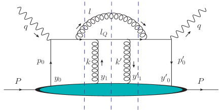
Figure 1: A representative single gluon emission diagram, where gluon emission is induced by single scattering.This represents a symmetric diagram with scattering off the final produced quark. Three separate cuts, denoted as central, left and right are indicated by the dashed lines.

In what follows, the focus will lie entirely on the hadronic tensor $W^{\mu\nu}$. We will carryout calculations of a set of contributions to $W^{\mu\nu}$ at next-to-leading order (NLO) as described above, and next-to-leading twist (NLT), meaning double scattering in the cross-section.

Already, at NLO and NLT, there are several interfering diagrams to consider. In this section, the calculation of one of the diagrams that contribute to single scattering induced single gluon emission will be carried out in some detail to familiarize the reader to the approximations carried out in this article. Figure (1) represents the diagram that will be evaluated. This diagram corresponds to the process where a semi-hard heavy quark produced after DIS radiates a gluon followed by a scattering in the medium, and finally exits the nucleus.

In this study, calculations will be carried out in axial gauge, $n\cdot A=0$, with $n\equiv(1,0,0_{\perp})$ and $A^{-}=0$. In $A^{-}=0$ gauge, the double scattering of a quark radiating a gluon contains a total of nine central cut diagrams where the cut line lies between the two scatterings. It also contains seven left cut diagrams and seven right cut diagrams. In this section, the central cut diagram of Fig.[1] will be analyzed in detail. In this section and what follows, only the real contribution where the radiated gluon line has been cut will be considered. The entire contribution from virtual diagrams, which contain a quark gluon fluctuation either in the amplitude or complex conjugate, will be obtained using unitarity arguments.

This NLO-NLT contribution to the hadronic tensor may be expressed as,

$$W^{\mu\nu} = g^{4}(-g_{\perp}^{\mu\nu})\int\frac{d^{4}{y^{\prime}_{0}}d^{4}p_{i}^{\prime}}{(2\pi)^{4}}\frac{d^{4}{y^{\prime}_{1}}d^{4}k^{\prime}}{(2\pi)^{4}}\frac{d^{4}{y_{1}}d^{4}k}{(2\pi)^{4}}\frac{d^{4}{y_{0}}d^{4}p_{i}}{(2\pi)^{4}}\frac{d^{4}l}{(2\pi)^{4}}\frac{d^{4}l_{Q}}{(2\pi)^{4}}e^{ip^{\prime}_{i}y^{\prime}_{0}}e^{ik^{\prime}y^{\prime}_{1}}e^{-iky_{1}}e^{-ip_{i}y_{0}}$$ (11)

$$\times{\rm Tr}\left[\frac{1}{2}\gamma^{-}\frac{-i({p\!\!\!/}_{f}+M)}{p_{f}^{2}-M^{2}-i\epsilon}\gamma_{\alpha}\frac{-i({p\!\!\!/}_{f}-{l\!\!\!/}+M)}{(p_{f}-l)^{2}-M^{2}-i\epsilon}{l\!\!\!/}_{q}G^{\alpha\beta}\frac{i({p\!\!\!/}_{f}-{l\!\!\!/}+M)}{(p_{f}-l)^{2}-M^{2}+i\epsilon}\gamma_{\beta}\frac{i({p\!\!\!/}_{f}-{l\!\!\!/}+M)}{(p_{f}-l)^{2}-M^{2}+i\epsilon}\right]$$

$$\times 2\pi\delta(l^{2})2\pi\delta(l_{Q}^{2}-M^{2})(-iT^{a})(iT^{a})\langle A|{\bar{\psi}}(y_{0}^{\prime})\gamma^{+}A^{+}(y_{1}^{\prime})A^{+}(y_{1})\psi(y_{0})|A\rangle.$$

We have defined the following momentum fractions for convenience,

$$y = \frac{l^{-}}{q^{-}}~{},~{}~{}\eta=\frac{k^{-}}{l^{-}}~{},~{}~{}\zeta=\frac{1-y}{1-y+\eta y}~{},$$ (12)

$$x_{0} = \frac{p_{i}^{+}}{P^{+}}~{},~{}~{}x_{1}=\frac{k^{+}}{P^{+}}~{},~{}~{}\chi=\frac{y^{2}M^{2}}{l_{\perp}^{2}}~{},$$

$$x_{L} = \frac{l_{\perp}^{2}}{2P^{+}q^{-}y(1-y)}~{},~{}~{}x_{D}=\frac{k_{\perp}^{2}-2l_{\perp}k_{\perp}}{2P^{+}q^{-}}~{}~{},~{}$$

$$x_{K} = \frac{k_{\perp}^{2}}{2P^{+}q^{-}}~{},~{}~{}\kappa=\frac{1}{1+(1-y)^{2}}~{},~{}~{}x_{M}=\frac{M^{2}}{2P^{+}q^{-}}.$$

In what follows, we will simply both numerator and denominator by retaining only leading terms in the $\lambda$ power counting highlighted above. This is followed by taking the trace in the numerator and contour integrations to simplify the denominator.

The factor $G^{\alpha\beta}$ is the polarization tensor, and in $A^{-}=~{}\!\!0$ gauge, it has the form,

$$G^{\alpha\beta}=-g^{\alpha\beta}+\frac{n^{\alpha}l^{\beta}+n^{\beta}l^{\alpha}}{nl}.$$ (13)

The structure of $n\equiv(1,0,0_{\perp})$ implies $n\cdot l=l^{-}$. Within this kinematic set up, in $A^{-}=0$ gauge, the leading component of the gluon field is $A^{+}$.

The spin sum in the numerator, containing the entire set of $\gamma$ matrices from the quark propagators, together with those from the interaction with the gauge field may be partially simplified and expressed as,

$${{\cal N}_{11}^{c}} = {\rm Tr}\left[\frac{1}{2}\gamma^{-}\left\{\gamma^{+}q^{-}\gamma_{\mu}\frac{n^{\mu}(l_{\perp})^{\nu}}{l^{-}}\gamma^{+}\left(q^{-}-l^{-}\right)+\gamma_{\perp}^{\alpha}{{p_{f}}_{\perp}}_{\alpha}{\gamma_{\perp}}_{\mu}\left(-g_{\perp}^{\mu\nu}\right)\gamma^{+}\left(q^{-}-l^{-}\right)\right.\right.$$ (14)

$$\left.\left.+\gamma^{+}q^{-}{\gamma_{\perp}}_{\mu}\left(-g_{\perp}^{\mu\nu}\right)\gamma_{\perp}^{\alpha}\left({p_{f}}_{\perp}-l_{\perp}\right)_{\alpha}\right\}\gamma^{-}\gamma^{+}(q^{-}-l^{-}+k^{-})\gamma^{-}\left\{\gamma^{+}(q^{-}-l^{-})\gamma_{\rho}\frac{n^{\rho}(l_{\perp})_{\nu}}{l^{-}}\gamma^{+}q^{-}\right.\right.$$

$$\left.\left.+\gamma^{+}(q^{-}-l^{-})\gamma_{\perp}^{\rho}(-g_{\perp})_{\rho\nu}\gamma_{\perp}^{\beta}{{p_{f}}_{\perp}}_{\beta}+\gamma_{\perp}^{\beta}\left({p_{f}}_{\perp}-l_{\perp}\right)_{\beta}\gamma_{\perp}^{\rho}(-g_{\perp})_{\rho\nu}\gamma^{+}q^{-}\right\}\right]$$

$$~{}+{\rm Tr}\left[\frac{1}{2}\gamma^{-}\left\{M{\gamma_{\perp}}_{\mu}\left(-g_{\perp}^{\mu\nu}\right)\gamma^{+}\left(q^{-}-l^{-}\right)+\gamma^{+}q^{-}{\gamma_{\perp}}_{\mu}\left(-g_{\perp}^{\mu\nu}\right)M\right\}\right.$$

$$\left.~{}\times\gamma^{-}\gamma^{+}(q^{-}-l^{-}+k^{-})\gamma^{-}\left\{\gamma^{+}(q^{-}-l^{-})\gamma_{\perp}^{\rho}(-g_{\perp})_{\rho\nu}M+M\gamma_{\perp}^{\rho}(-g_{\perp})_{\rho\nu}\gamma^{+}q^{-}\right\}\right].$$

Note that terms containing ${\gamma^{-}p_{f}^{+}}$ never contribute to the trace because there is always an adjacent factor of $\gamma^{-}$, and $\gamma^{-}\gamma^{-}=\gamma^{+}\gamma^{+}=0$. One may evaluate the trace, using the relation $\gamma^{+}\gamma^{-}=2-\gamma^{-}\gamma^{+}$ Eq.(14) simplifies to,

$${{\cal N}_{11}^{c}} = \frac{2(2q^{-})^{3}}{y}\left(1-y+y\eta\right)\left[P(y)l_{\perp}^{2}+y^{4}M^{2}\right].$$ (15)

Note that the mass independent portion contains the standard vacuum splitting function $P(y)$ while the mass dependent part has a separate dependence on the momentum fraction of the radiated gluon ($y$). In the soft emission kinematic limit where $y\ll 1$, one may neglect the mass term. However, in this work we will retain it throughout.

The set of denominators can now be evaluated using contour integration. For the central cut diagram of Fig.(1), this yields the phase factor,

$${\bar{I}}_{11}^{c} = \exp\left[i\left(x_{B}+x_{L}+\frac{x_{M}}{1-y}\right)P^{+}\left({y^{\prime}}^{-}_{0}-y_{0}^{-}\right)\right]\exp\left[i\left(\zeta x_{D}+\left(\zeta-1\right)\frac{x_{M}}{1-y}-\zeta\frac{\eta y^{2}}{1-y}x_{L}\right)P^{+}\left({y^{\prime}}^{-}_{1}-y^{-}_{1}\right)\right]$$

$$\times \theta\left(y^{-}_{1}-y^{-}_{0}\right)\theta\left({y^{\prime}}^{-}_{1}-{y^{\prime}}^{-}_{0}\right)$$

$$\times \left[1-\exp\left[-i\left(x_{L}+\frac{y}{1-y}x_{M}\right)P^{+}\left(y_{1}^{-}-y_{0}^{-}\right)\right]\right]\left[1-\exp\left[i\left(x_{L}+\frac{y}{1-y}x_{M}\right)P^{+}\left({y^{\prime}}^{-}_{1}-{y^{\prime}}^{-}_{0}\right)\right]\right].$$

This single diagram contains four contributions depending on the one propagator that remains off shell after contour integration.

Multiplying through we find four terms similar to the work of Ref. Wang:2001ifa . The first term where the same propagator is off-shell in both amplitude and complex conjugate corresponds to the so called “hard-soft” process where the gluon radiation is induced by the initial hard scattering. The heavy quark is knocked off-shell by the initial hard scattering and becomes on-shell after radiating the on-shell gluon. Afterwards, the on-shell quark or gluon will have a scattering with another soft medium gluon from the nucleus. The second term is the case where the quark is on-shell immediately after the first hard scattering. Gluon radiation is induced by subsequent scattering of the heavy quark off a in-medium gluon which carries a specific finite momentum fraction. This is often referred to as “hard-hard” scattering. The two cross terms where different propagators are off-shell in the amplitude and complex conjugate represent interference between soft-hard and hard-hard scatterings.

The equations derived above contain both longitudinal and transverse momentum exchanges with the medium. The portion due to transverse exchange may be isolated by imposing that $k^{-}\rightarrow 0~{}(\eta\rightarrow 0,~{}\zeta\rightarrow 1)$ limit, and then comparing with expressions from similar diagrams in Ref Zhang:2004qm . One will immediately note that factors containing $x_{M}$ which contribute to the Landau-Pomeranchuck-Migdal (LPM) Landau:1953um ; Migdal:1956tc effect are not modified by factors of $k^{-}$, while factors containing $x_{D}$ are modified by the presence of $k^{-}$. Factors of $x_{D}$ will eventually be absorbed in the definition of the transport coefficients including $\hat{q}$. Such factors introduce a non-trivial dependence of in-medium transport coefficients on the mass of the probe.

In this section, we have demonstrated how a certain diagram for heavy quark production and energy loss via gluon radiation can be simplified. Similar rules will be applied to all other real diagrams which include a cut of the radiated gluon line. In the subsequent section, all real diagrams will be combined to obtain the real gluon emission spectrum from a heavy quark that undergoes one scattering and one emission after production.

IV gluon emission spectrum

In the preceding section we evaluated the diagram in Fig. 1, in some detail, to highlight the approximations that will be made in the course of the full calculation. In this section, the result of the sum of all real diagrams (with an emitted gluon in the final state), will be presented. This will be followed by a gradient expansion in the exchanged transverse momentum ($k_{\perp}\rightarrow 0$). While the leading term in the limit of $k_{\perp}\rightarrow 0$, will correspond to a gauge correction to the vacuum process of gluon radiation from a heavy quark, the focus in this section will be on first correction in the $k_{\perp}\rightarrow 0$ limit, usually denoted as the next-to-leading twist contribution.

In total, there are 11 separate topologically distinct diagrams similar to that in Fig. 1. We denote these with two subscripts: $m,n=1$-$3$, where, $m$ denotes the location of the scattering in the amplitude, and $n$ denotes the location in the complex conjugate, for the case of a central cut, where one gluon scattering is on either side of the cut line. In either case of $m$ or $n$, $1$ signifies that the scattering occurs on the quark line beyond emission, $2$ signifies scattering on the quark line between the hard production and the emission, and $3$ signifies scattering of the emitted gluon. Each one of these diagrams will also generate a left and right cut component, where the cut line will be moved to the left or right of the scatterings, with the topology of the diagram held fixed. There are also the two special configurations, where both scatterings occur between the hard production and the gluon emission in the amplitude or complex-conjugate. These are denoted as $\mathcal{C}_{0,1}$ and $\mathcal{C}_{1,0}$. The next-to-leading twist portion, of the sum over all three cuts, for each of these contributions is outlined in the appendix.

Adding all the contributions from all the diagrams, categorized in the Appendix, we obtain the entire contribution to the hadronic tensor. In what follows, we decompose the hadronic tensor as,

$$W^{\mu\nu}=g^{4}2\pi(-g_{\perp}^{\mu\nu}){\cal H}^{c,l,r}.$$ (16)

The entire contribution from all real diagrams is contained in the factor $\mathcal{H}^{c,l,r}$. This, includes the initial hard scattering, the final state scattering of the quark or gluon, and the emission vertex. Virtual contributions, where the final state radiated gluon is not cut, will not be considered in this effort. Some part of the spin sum in the numerator has already been factorized out in the term $-g_{\perp}^{\mu\nu}$ above. In what follows, we will simplify ${\cal H}^{c,l,r}$ by factoring different contributions within it and then applying approximations to them separately. In the interest of readability, the exact details of the calculation for each diagram separately is included in the appendix.

This entire factor ${\cal H}^{c,l,r}$ is obtained as,

$${\cal H}^{c,l,r} = \sum_{m,n=1}^{3}{\cal C}_{m,n}^{c,l,r}+\mathcal{C}_{0,1}+\mathcal{C}_{1,0}=\frac{2\pi\alpha_{s}}{N_{c}}\int dl_{\perp}^{2}{H}^{c,l,r}$$ (17)

$$\times \exp\left[i\left(x_{B}+x_{L}+\frac{x_{M}}{1-y}\right)P^{+}\left({y^{\prime}}_{0}^{-}-{y}_{0}^{-}\right)\right.$$

$$+ i\left(\zeta x_{D}+\left(\zeta-1\right)\frac{x_{M}}{1-y}-\zeta\frac{\eta y^{2}}{1-y}x_{L}\right)$$

$$\times \left.P^{+}\left({y^{\prime}}_{1}^{-}-{y}_{1}^{-}\right)\right]$$

$$\times \langle A|{\bar{\psi}}(y_{0}^{\prime})\gamma^{+}A^{+}(y_{1}^{\prime})A^{+}(y_{1})\psi(y_{0})|A\rangle$$

In the equation above, cut specific phase factors and the hard part for each cut are entirely contained within ${H}^{c,l,r}$. The overall phase factor represents the generic portion of the phase factor.

In order to calculate the next-to-leading power contribution to the semi-inclusive hard partonic cross-section, one needs to expand the cross-section in $k_{\perp}$ and in $k^{-}$. In each case, we will extract the corresponding transport coefficients inside the gluon emission spectrum kernel for the semi-hard heavy quark Majumder:2009ge . Factors of $k_{\perp}$ and $k^{-}$ are absorbed as derivatives within the definition of the transport coefficients [e.g. $k_{\perp}A^{+}(\vec{y}_{\perp})\exp(i\vec{k}_{\perp}\cdot\vec{y}_{\perp})=-i\nabla_{\perp}A^{+}(\vec{y}_{\perp})\exp(i\vec{k}_{\perp}\cdot\vec{y}_{\perp})\simeq iF^{+\perp}(\vec{y}_{\perp})\exp(i\vec{k}_{\perp}\cdot\vec{y}_{\perp})$].

We will also factor the four point non-perturbative operator using the usual phenomenological factorization, which for the case of transverse scattering may be expressed as,

$$\langle A|{\bar{\psi}}(y_{0}^{\prime})\gamma^{+}F^{+}_{\perp}(y_{1}^{\prime})F^{+}_{\perp}(y_{1})\psi(y_{0})|A\rangle\simeq C^{A}_{p}$$ (18)

$$\times \langle p|{\bar{\psi}}(y_{0}^{\prime})\gamma^{+}\psi(y_{0})|p\rangle\frac{\rho}{2p^{+}}\langle p|F^{+}_{\perp}(y_{1}^{\prime})F^{+}_{\perp}(y_{1})|p\rangle.$$

The first operator product on the right hand side of the equation above will yield the incoming quark distribution function within one nucleon. The second operator product will yield the transport coefficient due to the scattering of the final state, off a gluon within a nucleon in the nucleus. We have assumed the average condition that both nucleons have a momentum $p=P/A$. The factor $\rho$ represents the nucleon density within the nucleus, and $C_{p}^{A}$ represents an overall normalization constant that contains the nucleon density. The factor of $\rho/(2p^{+})$ is written separately as that will be absorbed within the definition of the transport coefficient.

These transport coefficients, defined below, are non-perturbative objects, which are factorized from the hard part that describes the propagation of the heavy quark. While the exact value of each of these coefficients depends on the non-perturbative dynamics of the medium, the relative contributions of the different hard parts that appear as a multiplicative factor along with these coefficients will be calculated below. Terms for the transverse diffusion $\hat{q}$, the drag (and longitudinal diffusion) coefficient $\hat{e}$ ($\hat{e}_{2}$) can be obtained through derivatives of the kernel with respect to the transverse and $(-)$-light-cone component of the exchange momentum,

$$\left[\nabla_{k_{\perp}}^{2},\nabla_{k^{-}},\nabla_{k^{-}}^{2}\right]\left.{H}^{c,l,r}\right|_{k_{\perp},k^{-}=0}$$ (19)

$$= 4C_{A}\left(\frac{1+(1-y)^{2}}{y}\right)\frac{l_{\perp}^{4}}{[l_{\perp}^{2}+y^{2}M^{2}]^{4}}{\tilde{H}}_{c,l,r}^{{\hat{q}},{\hat{e}},{\hat{e}}_{2}}.$$

In the equation above, the factor ${\tilde{H}}_{c,l,r}^{{\hat{q}},{\hat{e}},{\hat{e}}_{2}}$ represents several terms, depending on the cut taken i.e., central $c$, left $l$, or right $r$, and the momentum component with respect to which the Taylor expansion is carried out, i.e., $\hat{q}$ for the second derivative in terms of $k_{\perp}$, $\hat{e}$ for the first derivative with respect to $k^{-}$ and $\hat{e}_{2}$ for the second derivative with respect to $k^{-}$. One should note that for each case, once the derivatives have been taken, both factors of the momentum $k_{\perp},k^{-}$ are set to zero. The complete expressions for $\tilde{H}_{c,l,r}^{{\hat{q}},{\hat{e}},{\hat{e}}_{2}}$ can be expressed as a sum of products of a phase factor and a non-phase factor coefficient, expressed as $c^{{\hat{q}},{\hat{e}},{\hat{e}}_{2}}_{n}$:

$${\tilde{H}}_{c}^{{\hat{q}},{\hat{e}},{\hat{e}}_{2}} = c_{1}^{{\hat{q}},{\hat{e}},{\hat{e}}_{2}}\left[1-e^{-i\left(x_{L}+\frac{y}{1-y}x_{M}\right)P^{+}\left({y}_{1}^{-}-{y}_{0}^{-}\right)}\right]\left[1-e^{i\left(x_{L}+\frac{y}{1-y}x_{M}\right)P^{+}\left({y^{\prime}}_{1}^{-}-{y^{\prime}}_{0}^{-}\right)}\right]+c_{2}^{{\hat{q}},{\hat{e}},{\hat{e}}_{2}}\left\{e^{-i\left(x_{L}+\frac{y}{1-y}x_{M}\right)P^{+}\left({y}_{1}^{-}-{y}_{0}^{-}\right)}\right.$$

$$\times \left.\left[1-e^{i\left(x_{L}+\frac{y}{1-y}x_{M}\right)P^{+}\left({y^{\prime}}_{1}^{-}-{y^{\prime}}_{0}^{-}\right)}\right]+\left[1-e^{-i\left(x_{L}+\frac{y}{1-y}x_{M}\right)P^{+}\left({y}_{1}^{-}-{y}_{0}^{-}\right)}\right]e^{i\left(x_{L}+\frac{y}{1-y}x_{M}\right)P^{+}\left({y^{\prime}}_{1}^{-}-{y^{\prime}}_{0}^{-}\right)}\right\}$$

$$+ c_{3}^{{\hat{q}},{\hat{e}},{\hat{e}}_{2}}\left[e^{-i\left(x_{L}+\frac{y}{1-y}x_{M}\right)P^{+}\left({y}_{1}^{-}-{y}_{0}^{-}\right)}\right]\left[e^{i\left(x_{L}+\frac{y}{1-y}x_{M}\right)P^{+}\left({y^{\prime}}_{1}^{-}-{y^{\prime}}_{0}^{-}\right)}\right],$$

$${\tilde{H}}_{l}^{{\hat{q}},{\hat{e}},{\hat{e}}_{2}} = c_{4}^{{\hat{q}},{\hat{e}},{\hat{e}}_{2}}\left[e^{-i\left(x_{L}+\frac{y}{1-y}x_{M}\right)P^{+}\left({y^{\prime}}_{0}^{-}-{y^{\prime}}_{1}^{-}\right)}-e^{-i\left(x_{L}+\frac{y}{1-y}x_{M}\right)P^{+}\left({y^{\prime}}_{0}^{-}-{y}_{1}^{-}\right)}\right]+c_{5}^{{\hat{q}},{\hat{e}},{\hat{e}}_{2}}\left[1-e^{-i\left(x_{L}+\frac{y}{1-y}x_{M}\right)P^{+}\left({y^{\prime}}_{0}^{-}-{y^{\prime}}_{1}^{-}\right)}\right],$$

$${\tilde{H}}_{r}^{{\hat{q}},{\hat{e}},{\hat{e}}_{2}} = c_{4}^{{\hat{q}},{\hat{e}},{\hat{e}}_{2}}\left[e^{-i\left(x_{L}+\frac{y}{1-y}x_{M}\right)P^{+}\left({y}_{0}^{-}-{y}_{1}^{-}\right)}-e^{-i\left(x_{L}+\frac{y}{1-y}x_{M}\right)P^{+}\left({y}_{0}^{-}-{y^{\prime}}_{1}^{-}\right)}\right]+c_{5}^{{\hat{q}},{\hat{e}},{\hat{e}}_{2}}\left[1-e^{-i\left(x_{L}+\frac{y}{1-y}x_{M}\right)P^{+}\left({y}_{0}^{-}-{y}_{1}^{-}\right)}\right].$$

In each case above, the coefficients $c_{n}^{{\hat{q}},{\hat{e}},{\hat{e}}_{2}}$ depend on the momentum component being considered. The subscript $n$ merely denotes the order in which the coefficient occurs: $c_{1}$, $c_{2}$ and $c_{3}$ appear in the expression for the central cut, where $c_{4}$ and $c_{5}$ appear in both the left and right cuts. We list them in the following for each different case, starting from the case of transverse diffusion, i.e., $\hat{q}$. The coefficients are,

$$c_{1}^{\hat{q}} = 1-(2-3\kappa y^{2})\chi+(1-\kappa y^{2})\chi^{2}~{},$$

$$c_{2}^{\hat{q}} = -\frac{y}{2}+\left[\left(1-\frac{1}{2}\kappa y^{2}-\kappa y^{3}\right)+y^{2}\frac{C_{F}}{C_{A}}\left(2-\kappa y^{2}\right)\right]\chi$$

$$-\left[\frac{1}{2}\left(y-\kappa y^{2}\right)-y^{2}\frac{C_{F}}{C_{A}}\left(\kappa y^{2}\right)\right]\chi^{2}~{},$$

$$c_{3}^{\hat{q}} = y^{2}\frac{C_{F}}{C_{A}}\left[1-4(1-\kappa y^{2})\chi+(1-2\kappa y^{2})\chi^{2}\right]~{},$$

$$c_{4}^{\hat{q}} = \left[1+\frac{y^{2}}{1+(1-y)^{2}}\chi\right]\left[\frac{C_{F}}{C_{A}}y^{2}+1-2y\right]\chi~{},$$

$$c_{5}^{\hat{q}} = \left[1+\frac{y^{2}}{{1+(1-y)^{2}}}\chi\right]\chi~{}.$$ (20)

The momentum fractions $y$, $\kappa$ and $\chi$ are defined in Eq. (12). For the longitudinal drag coefficient $\hat{e}$, the $c$-factors are,

$$c_{1}^{\hat{e}} = \frac{y^{2}M^{2}}{l^{-}}\left[\frac{1}{2}+\frac{1}{2}(1+\kappa y^{2})\chi+\frac{1}{2}\chi^{2}\right],$$

$$c_{2}^{\hat{e}} = \frac{y^{2}M^{2}}{l^{-}}\left[-\frac{1}{4}-\frac{1}{4}(1+\kappa y^{2})~{}y^{2}\chi-\frac{1}{4}\chi^{2}\right],$$

$$c_{3}^{\hat{e}} = 0~{},c_{4}^{\hat{e}}=0~{},c_{5}^{\hat{e}}=0.$$

For longitudinal diffusion coefficient $\hat{e}_{2}$, the $c$-factors are,

$$c_{1}^{{\hat{e}}_{2}} = \frac{y^{2}M^{2}}{(l^{-})^{2}}\left[-\frac{1}{2}+\left(\frac{7}{2}-\frac{1}{2}\kappa y^{2}\right)\chi+\frac{7}{2}~{}y^{2}\chi^{2}\right],$$

$$c_{2}^{{\hat{e}}_{2}} = \frac{y^{2}M^{2}}{(l^{-})^{2}}\left[\frac{1}{4}-\left(\frac{3}{4}-\frac{1}{4}\kappa y^{2}\right)\chi-\frac{3}{4}\kappa y^{2}~{}\chi^{2}\right],$$

$$c_{3}^{{\hat{e}}_{2}} = 0~{},~{}~{}c_{4}^{{\hat{e}}_{2}}=0~{},~{}~{}c_{5}^{{\hat{e}}_{2}}=0~{}.$$

All the terms presented above can be combined to obtain the real single gluon emission spectrum. In the second line of the equation below [Eq. (21)], we have retained terms only up to ${\cal O}(\sqrt{\lambda})$, the approximation that has been justified in this study. All terms which scale as ${\cal O}(\lambda)$ or greater, have been neglected. We express the gluon spectrum per unit light-cone length as,

$$\frac{dN_{g}}{dydl^{2}_{\perp}d\tau} = 2~{}\frac{\alpha}{\pi}~{}P(y)~{}\frac{1}{l^{4}_{\perp}}\left(\frac{1}{1+\chi}\right)^{4}~{}\sin^{2}\left(\frac{l^{2}_{\perp}}{4l^{-}(1-y)}(1+\chi)~{}\tau\right)\left[\left\{c_{1}^{\hat{q}}+c_{2}^{\hat{q}}\right\}~{}{\hat{q}}+4\left\{c_{1}^{\hat{e}}+c_{2}^{\hat{e}}\right\}~{}{\hat{e}}+2\left\{c_{1}^{{\hat{e}}_{2}}+c_{2}^{{\hat{e}}_{2}}\right\}~{}{\hat{e}_{2}}\right]$$ (21)

$$= 2~{}\frac{\alpha}{\pi}~{}P(y)~{}\frac{1}{l^{4}_{\perp}}\left(\frac{1}{1+\chi}\right)^{4}~{}\sin^{2}\left(\frac{l^{2}_{\perp}}{4l^{-}(1-y)}(1+\chi)~{}\tau\right)$$

$$\times \left[\left\{\left(1-\frac{y}{2}\right)-\chi+\left(1-\frac{y}{2}\right)\chi^{2}\right\}~{}{\hat{q}}+\frac{l_{\perp}^{2}}{l^{-}}\chi\left(1+\chi\right)^{2}~{}{\hat{e}}+\frac{l_{\perp}^{2}}{(l^{-})^{2}}\chi\left(\frac{1}{2}-\frac{11}{4}\chi\right){\hat{e}_{2}}\right].$$

In the equation above, we have defined a mean light-cone location of the first scattering (between the amplitude and complex conjugate) as

$$\tau=\frac{y_{1}^{-}+{y^{\prime}}_{1}^{-}}{2}.$$ (22)

We also define the off-set between the light cone locations in the amplitude and complex-conjugate as,

$$y^{-}=y_{1}^{-}-{y^{\prime}}_{1}^{-}.$$ (23)

This variable enters the definitions of all transport coefficients that will be discussed in this paper. There are three transport coefficients, which contain the non-perturbative expection of the gluon field strength operators: the transverse diffusion coefficient, $\hat{q}$ which represents the transverse momentum squared per unit light-cone length, exchanged between the hard quark and the medium, the longitudinal drag per unit light-cone length, $\hat{e}$ caused due to the exchange of light-cone components of momentum, and $\hat{e}_{2}$ the diffusion in light-cone momentum, per unit light-cone length :

$${\hat{q}} = \frac{4\pi^{2}C_{R}\alpha_{s}}{N_{C}^{2}-1}\int\frac{dy^{-}}{\pi}\frac{\rho}{2p^{+}}$$

$$\times \langle A|F_{\perp}^{~{}+}(y^{-})F^{\perp+}(0)|A\rangle~{}e^{-i{\bar{\Delta}}P^{+}y^{-}},$$

$${\hat{e}} = \frac{4\pi^{2}C_{R}\alpha_{s}}{N_{C}^{2}-1}\int\frac{dy^{-}}{\pi}\frac{\rho}{2p^{+}}$$

$$\times \langle A|i\partial^{-}A^{+}(y^{-})A^{+}(0)|A\rangle~{}e^{-i{\bar{\Delta}}P^{+}y^{-}},$$

$${\hat{e}_{2}} = \frac{4\pi^{2}C_{R}\alpha_{s}}{N_{C}^{2}-1}\int\frac{dy^{-}}{\pi}\frac{\rho}{2p^{+}}$$ (24)

$$\times \langle A|F^{-+}(y^{-})F^{-+}(0)|A\rangle~{}e^{-i{\bar{\Delta}}P^{+}y^{-}}.$$

In the equations above, we observe the appearance of another momentum fraction:

$$\bar{\Delta} = \zeta x_{D}+\left(\zeta-1\right)\frac{x_{M}}{1-y}-\zeta\frac{\eta y^{2}}{1-y}x_{L}~{}.$$ (25)

The presence of such a momentum fraction, indicates that the range of momentum fractions in the definition of $\hat{q}$ $\hat{e}$ and $\hat{e}_{2}$ for heavy quark scattering is different from that for light flavor energy loss. This indicates that the actual value of $\hat{q}$ (or even $\hat{e}$ or $\hat{e}_{2}$) for heavy quarks may be different from that for light quarks. Thus, careful analysis of heavy-quark energy loss may lead to an understanding of the $x$-dependence of the in-medium gluon distribution function that sources transport coefficients, and may, in the end, lead to an understanding of the degrees of freedom within dense media, where heavy quark energy loss is carried out.

V Conclusion and Outlook

In this work, the gluon bremsstrahlung from a “semi-hard” heavy quark in a dense nuclear medium has been studied in greater detail than in several earlier efforts. In this work, we have considered a hard virtual photon scattering off a hard heavy quark (within a proton), that converts it to a slow moving heavy quark that moves through the remainder of the nucleus before escaping and fragmenting into a jet containing a heavy meson.

In this work both transverse broadening as well as the longitudinal drag and longitudinal diffusion, have been studied on an equal footing. We have categorically focussed our study on “semi-hard” quarks where the mass and momentum scale as $M,p\sim\sqrt{\lambda}Q$, as these are the quarks for which mass modifications is most prominent. We have used power counting arguments loosely based on Soft Collinear Effective Theory (SCET) at various stage to isolate the leading contributions. It was shown in our earlier studies that both longitudinal and transverse momentum transfers have a comparable effect on the off-shellness of the heavy-quark Abir:2014sxa . This earlier work implied that longitudinal transfers, not only lead to the drag and diffusion, similar to light flavors, but will also noticeably affect the radiative loss and left strong indications that for heavy quarks, the drag induced radiation may be as significant as transverse momentum diffusion ($\hat{q}$) induced radiation.

In this paper we have explicitly demonstrated that the gluon bremsstrahlung spectrum from a semi-hard heavy quark is indeed strongly modified by drag induced radiation. We have shown that due to the presence of the $(-)$-light-cone momentum exchange from the medium ($k^{-}$), in our calculations, the definition of all the transport coefficients for heavy quark is different from that for light quark. Thus transport coefficients may indeed depend on properties of the probe i.e. mass or on the $l_{\perp}^{2}$. Whether this is phenomenologically significant cannot be ascertained at this point, and is left for a future investigation. This explicit dependence on the $(-)$-light cone momentum was absent in the limit of $k^{-}\rightarrow 0$, assumed in several prior calculations.

The implications of the present study on the phenomenology of HIC is under way. It this work we have shown that the gluon bremsstrahlung spectrum of heavy quark (unlike light quark) is parametrically sensitive to $\hat{e}$ which quantifies the amount of drag the moving quark experiences. This result can be used to estimate the value of this sub-leading non-perturbative jet transport parameter ($\hat{e}$) from heavy flavor data of HIC experiments. These extra additive contributions may lead to an eventual solution of the heavy quark puzzle. We leave these for a future effort.

VI Acknowledgments

The authors would like to thank G.-Y. Qin for many helpful discussions. This work was supported in part by the National Science Foundation under grant number PHY-1207918. This work is also supported in part by the Director, Office of Energy Research, Office of High Energy and Nuclear Physics, Division of Nuclear Physics, of the U.S. Department of Energy, through the JET topical collaboration.

VII Appendix

Figure 2:

There are three different cuts (central, left and right) in Fig.[2] and their contributions are,

$${\cal C}_{11}^{c,l,r} = \frac{\alpha_{s}^{2}}{N_{c}}\left[C_{F}\right]\int dl_{\perp}^{2}\left(\frac{1+(1-y)^{2}}{y}\right)\frac{[l_{\perp}^{2}+\kappa y^{4}M^{2}]}{(l_{\perp}^{2}+y^{2}M^{2})^{2}}~{}{\bar{I}}_{11}^{c,l,r}$$ (26)

$${\bar{I}}_{11}^{c} = \exp\left[i\left(x_{B}+x_{L}+\frac{x_{M}}{1-y}\right)P^{+}\left({y^{\prime}}_{0}^{-}-{y}_{0}^{-}\right)\right]\exp\left[i\left(\zeta x_{D}+\left(\zeta-1\right)\frac{x_{M}}{1-y}-\zeta\frac{\eta y^{2}}{1-y}x_{L}\right)P^{+}\left({y^{\prime}}_{1}^{-}-{y}_{1}^{-}\right)\right]\theta\left({y}_{0}^{-}-{y}_{1}^{-}\right)$$

$$\times~{}\theta\left({y^{\prime}}_{0}^{-}-{y^{\prime}}_{1}^{-}\right)\left[1-\exp\left[-i\left(x_{L}+\frac{y}{1-y}x_{M}\right)P^{+}\left({y}_{1}^{-}-{y}_{0}^{-}\right)\right]\right]\left[1-\exp\left[i\left(x_{L}+\frac{y}{1-y}x_{M}\right)P^{+}\left({y^{\prime}}_{1}^{-}-{y^{\prime}}_{0}^{-}\right)\right]\right]$$

$${\bar{I}}_{11}^{l} = \exp\left[i\left(x_{B}+x_{L}+\frac{x_{M}}{1-y}\right)P^{+}\left({y^{\prime}}_{0}^{-}-{y}_{0}^{-}\right)\right]\exp\left[i\left(\zeta x_{D}+\left(\zeta-1\right)\frac{x_{M}}{1-y}-\zeta\frac{\eta y^{2}}{1-y}x_{L}\right)P^{+}\left({y^{\prime}}_{1}^{-}-{y}_{1}^{-}\right)\right]$$ (28)

$$\times~{}\theta\left({y^{\prime}}_{1}^{-}-{y}_{1}^{-}\right)\theta\left({y^{\prime}}_{0}^{-}-{y^{\prime}}_{1}^{-}\right)\left(-1\right)\left[1-\exp\left[i\left(x_{L}+\frac{y}{1-y}x_{M}\right)P^{+}\left({y^{\prime}}_{1}^{-}-{y^{\prime}}_{0}^{-}\right)\right]\right]$$

$${\bar{I}}_{11}^{c} = \exp\left[i\left(x_{B}+x_{L}+\frac{x_{M}}{1-y}\right)P^{+}\left({y^{\prime}}_{0}^{-}-{y}_{0}^{-}\right)\right]\exp\left[i\left(\zeta x_{D}+\left(\zeta-1\right)\frac{x_{M}}{1-y}-\zeta\frac{\eta y^{2}}{1-y}x_{L}\right)P^{+}\left({y^{\prime}}_{1}^{-}-{y}_{1}^{-}\right)\right]\theta\left(y_{0}^{-}-y_{1}^{-}\right)$$ (29)

$$\times~{}\theta\left({y}_{1}^{-}-{y^{\prime}}_{1}^{-}\right)\left[1-\exp\left[-i\left(x_{L}+\frac{y}{1-y}x_{M}\right)P^{+}\left({y}_{1}^{-}-{y}_{0}^{-}\right)\right]\right]\left(-1\right)$$

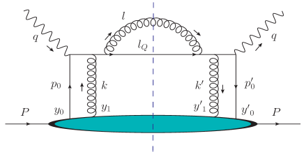
Figure 3:

In Fig.[3] there are only central cut, with the contribution,

$${\cal C}_{22}^{c} = \frac{\alpha_{s}^{2}}{N_{c}}\left[C_{F}\right]\int dl_{\perp}^{2}\left(\frac{1+\eta y+(1-y+\eta y)^{2}}{y}\right)\frac{[\left[(1+\eta y)l_{\perp}-yk_{\perp}\right]^{2}+\kappa y^{4}M^{2}]}{\left[\left(l_{\perp}-yk_{\perp}\right)^{2}+y^{2}M^{2}+2y\eta\left(l_{\perp}^{2}-l_{\perp}k_{\perp}\right)+y^{2}\eta^{2}l_{\perp}^{2}\right]^{2}}~{}{\bar{I}}_{11}^{c,l,r}$$ (30)

$${\bar{I}}_{22}^{c} = \exp\left[i\left(x_{B}+x_{L}+\frac{x_{M}}{1-y}\right)P^{+}\left({y^{\prime}}_{0}^{-}-{y}_{0}^{-}\right)\right]\exp\left[i\left(\zeta x_{D}+\left(\zeta-1\right)\frac{x_{M}}{1-y}-\zeta\frac{\eta y^{2}}{1-y}x_{L}\right)P^{+}\left({y^{\prime}}_{1}^{-}-{y}_{1}^{-}\right)\right]\theta\left({y}_{0}^{-}-{y}_{1}^{-}\right)$$ (31)

$$\times~{}\theta\left({y^{\prime}}_{0}^{-}-{y^{\prime}}_{1}^{-}\right)\left[-\exp\left[-i\left(x_{L}+\frac{y}{1-y}x_{M}\right)P^{+}\left({y}_{1}^{-}-{y}_{0}^{-}\right)\right]\right]\left[-\exp\left[i\left(x_{L}+\frac{y}{1-y}x_{M}\right)P^{+}\left({y^{\prime}}_{1}^{-}-{y^{\prime}}_{0}^{-}\right)\right]\right]$$

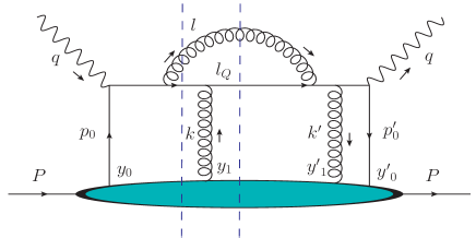
Figure 4:

In Fig.[4] there are two different cuts for induced gluon radition, central and left.

$${\cal C}_{12}^{c,l} = \frac{\alpha_{s}^{2}}{N_{c}}\left[-\left(C_{F}-\frac{C_{A}}{2}\right)\right]\int dl_{\perp}^{2}\left(\frac{1+(1-y)^{2}+\eta y(2-y)}{y}\right)$$ (32)

$$\times~{}\frac{[l_{\perp}\left[(1+\eta y)l_{\perp}-yk_{\perp}\right]+\kappa y^{4}M^{2}]}{[l_{\perp}^{2}+y^{2}M^{2}]\left[\left(l_{\perp}-yk_{\perp}\right)^{2}+y^{2}M^{2}+2y\eta\left(l_{\perp}^{2}-l_{\perp}k_{\perp}\right)+y^{2}\eta^{2}l_{\perp}^{2}\right]}{\bar{I}}_{12}^{c,l}$$

$${\bar{I}}_{12}^{c} = \exp\left[i\left(x_{B}+x_{L}+\frac{x_{M}}{1-y}\right)P^{+}\left({y^{\prime}}_{0}^{-}-{y}_{0}^{-}\right)\right]\exp\left[i\left(\zeta x_{D}+\left(\zeta-1\right)\frac{x_{M}}{1-y}-\zeta\frac{\eta y^{2}}{1-y}x_{L}\right)P^{+}\left({y^{\prime}}_{1}^{-}-{y}_{1}^{-}\right)\right]\theta\left({y}_{0}^{-}-{y}_{1}^{-}\right)$$

$$\times~{}\theta\left({y^{\prime}}_{0}^{-}-{y^{\prime}}_{1}^{-}\right)\left[1-\exp\left[-i\left(x_{L}+\frac{y}{1-y}x_{M}\right)P^{+}\left({y}_{1}^{-}-{y}_{0}^{-}\right)\right]\right]\left[-\exp\left[i\left(x_{L}+\frac{y}{1-y}x_{M}\right)P^{+}\left({y^{\prime}}_{1}^{-}-{y^{\prime}}_{0}^{-}\right)\right]\right]$$

$${\bar{I}}_{12}^{l} = \exp\left[i\left(x_{B}+x_{L}+\frac{x_{M}}{1-y}\right)P^{+}\left({y^{\prime}}_{0}^{-}-{y}_{0}^{-}\right)\right]\exp\left[i\left(\zeta x_{D}+\left(\zeta-1\right)\frac{x_{M}}{1-y}-\zeta\frac{\eta y^{2}}{1-y}x_{L}\right)P^{+}\left({y^{\prime}}_{1}^{-}-{y}_{1}^{-}\right)\right]$$ (34)

$$\times~{}\theta\left({y^{\prime}}_{1}^{-}-{y}_{1}^{-}\right)\theta\left({y^{\prime}}_{0}^{-}-{y^{\prime}}_{1}^{-}\right)\left[\exp\left[i\left(x_{L}+\frac{y}{1-y}x_{M}\right)P^{+}\left({y}_{1}^{-}-{y^{\prime}}_{0}^{-}\right)+i\left(x_{K}-x_{D}\right)P^{+}\left({y^{\prime}}_{1}^{-}-y_{1}^{-}\right)\right]\right.$$

$$\left.-\exp\left[i\left(x_{L}+\frac{y}{1-y}x_{M}\right)P^{+}\left({y^{\prime}}_{1}^{-}-{y^{\prime}}_{0}^{-}\right)\right]\right]$$

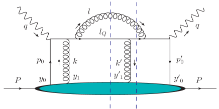
Figure 5:

In Fig.[5] there are two different cuts for induced gluon radition, central and right.

$${\cal C}_{21}^{c,r} = \frac{\alpha_{s}^{2}}{N_{c}}\left[-\left(C_{F}-\frac{C_{A}}{2}\right)\right]\int dl_{\perp}^{2}\left(\frac{1+(1-y)^{2}+\eta y(2-y)}{y}\right)$$

$$\times~{}\frac{[\left[(1+\eta y)l_{\perp}-yk_{\perp}\right]l_{\perp}+\kappa y^{4}M^{2}]}{\left[\left(l_{\perp}-yk_{\perp}\right)^{2}+y^{2}M^{2}+2y\eta\left(l_{\perp}^{2}-l_{\perp}k_{\perp}\right)+y^{2}\eta^{2}l_{\perp}^{2}\right][l_{\perp}^{2}+y^{2}M^{2}]}{\bar{I}}_{21}^{c,r}$$

$${\bar{I}}_{21}^{c} = \exp\left[i\left(x_{B}+x_{L}+\frac{x_{M}}{1-y}\right)P^{+}\left({y^{\prime}}_{0}^{-}-{y}_{0}^{-}\right)\right]\exp\left[i\left(\zeta x_{D}+\left(\zeta-1\right)\frac{x_{M}}{1-y}-\zeta\frac{\eta y^{2}}{1-y}x_{L}\right)P^{+}\left({y^{\prime}}_{1}^{-}-{y}_{1}^{-}\right)\right]\theta\left({y}_{0}^{-}-{y}_{1}^{-}\right)$$

$$\times~{}\theta\left({y^{\prime}}_{0}^{-}-{y^{\prime}}_{1}^{-}\right)\left[-\exp\left[-i\left(x_{L}+\frac{y}{1-y}x_{M}\right)P^{+}\left({y}_{1}^{-}-{y}_{0}^{-}\right)\right]\right]\left[1-\exp\left[i\left(x_{L}+\frac{y}{1-y}x_{M}\right)P^{+}\left({y^{\prime}}_{1}^{-}-{y^{\prime}}_{0}^{-}\right)\right]\right]$$

$${\bar{I}}_{21}^{r} = \exp\left[i\left(x_{B}+x_{L}+\frac{x_{M}}{1-y}\right)P^{+}\left({y^{\prime}}_{0}^{-}-{y}_{0}^{-}\right)\right]\exp\left[i\left(\zeta x_{D}+\left(\zeta-1\right)\frac{x_{M}}{1-y}-\zeta\frac{\eta y^{2}}{1-y}x_{L}\right)P^{+}\left({y^{\prime}}_{1}^{-}-{y}_{1}^{-}\right)\right]$$ (36)

$$\times~{}\theta\left({y}_{1}^{-}-{y^{\prime}}_{1}^{-}\right)\theta\left({y}_{0}^{-}-{y}_{1}^{-}\right)\left[\exp\left[-i\left(x_{L}+\frac{y}{1-y}x_{M}\right)P^{+}\left({y^{\prime}}_{1}^{-}-{y}_{0}^{-}\right)-i\left(x_{K}-x_{D}\right)P^{+}\left({y}_{1}^{-}-{y^{\prime}}_{1}^{-}\right)\right]\right.$$

$$\left.-\exp\left[-i\left(x_{L}+\frac{y}{1-y}x_{M}\right)P^{+}\left({y}_{1}^{-}-{y}_{0}^{-}\right)\right]\right]$$

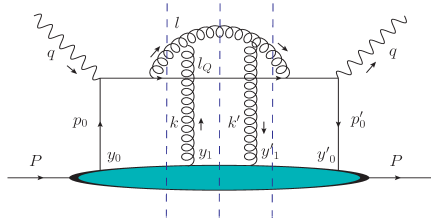
Figure 6:

In Fig.[6] there are again all three possible cuts for induced gluon radition,

$${\cal C}_{33}^{c} = \frac{\alpha_{s}^{2}}{N_{c}}\left[C_{A}\right]\int dl_{\perp}^{2}P(y)\frac{[\left(l_{\perp}-k_{\perp}\right)^{2}+\kappa y^{4}M^{2}]}{[\left(l_{\perp}-k_{\perp}\right)^{2}+\left(1-\eta\right)^{2}y^{2}M^{2}]^{2}}{\bar{I}}_{33}^{c}$$

$${\bar{I}}_{33}^{c} = \exp\left[i\left(x_{B}+x_{L}+\frac{x_{M}}{1-y}\right)P^{+}\left({y^{\prime}}_{0}^{-}-{y}_{0}^{-}\right)\right]\exp\left[i\left(\zeta x_{D}+\left(\zeta-1\right)\frac{x_{M}}{1-y}-\zeta\frac{\eta y^{2}}{1-y}x_{L}\right)P^{+}\left({y^{\prime}}_{1}^{-}-{y}_{1}^{-}\right)\right]\theta\left({y}_{0}^{-}-{y}_{1}^{-}\right)$$ (37)

$$\times~{}\theta\left({y^{\prime}}_{0}^{-}-{y^{\prime}}_{1}^{-}\right)\left[\exp\left\{i\left(\frac{\zeta}{y(1-\eta)}x_{D}+\frac{\eta(1-y)}{\left(1-\eta\right)}x_{L}+\left(\zeta-1\right)\frac{x_{M}}{1-y}-\zeta\frac{\eta y^{2}}{1-y}x_{L}\right)P^{+}\left(y_{1}^{-}-y_{0}^{-}\right)\right\}\right.$$

$$\left.-\exp\left[-i\left(x_{L}+\frac{y}{1-y}x_{M}\right)P^{+}\left({y}_{1}^{-}-{y}_{0}^{-}\right)\right]\right]\left[\exp\left\{-i\left(\frac{\zeta}{y(1-\eta)}x_{D}+\frac{\eta(1-y)}{\left(1-\eta\right)}x_{L}+\left(\zeta-1\right)\frac{x_{M}}{1-y}-\zeta\frac{\eta y^{2}}{1-y}x_{L}\right)\right.\right.$$

$$\left.\left.\times~{}P^{+}\left({y^{\prime}}_{1}^{-}-{y^{\prime}}_{0}^{-}\right)\right\}-\exp\left[i\left(x_{L}+\frac{y}{1-y}x_{M}\right)P^{+}\left({y^{\prime}}_{1}^{-}-{y^{\prime}}_{0}^{-}\right)\right]\right]$$

$${\cal C}_{33}^{l,r} = \frac{\alpha_{s}^{2}}{N_{c}}\left[C_{A}\right]\int dl_{\perp}^{2}P(y)\frac{l_{\perp}^{2}+\kappa y^{4}M^{2}}{[l_{\perp}^{2}+y^{2}M^{2}]^{2}}{\bar{I}}_{33}^{l,r}$$

$${\bar{I}}_{33}^{l} = \exp\left[i\left(x_{B}+x_{L}+\frac{x_{M}}{1-y}\right)P^{+}\left({y^{\prime}}_{0}^{-}-{y}_{0}^{-}\right)\right]\exp\left[i\left(\zeta x_{D}+\left(\zeta-1\right)\frac{x_{M}}{1-y}-\zeta\frac{\eta y^{2}}{1-y}x_{L}\right)P^{+}\left({y^{\prime}}_{1}^{-}-{y}_{1}^{-}\right)\right]\theta\left({y^{\prime}}_{1}^{-}-{y}_{1}^{-}\right)$$ (38)

$$\times~{}\theta\left({y^{\prime}}_{0}^{-}-{y^{\prime}}_{1}^{-}\right)\left[-\exp\left\{i\left(\frac{-\zeta(1-2y(1-\eta))}{y(1-\eta)}x_{D}-\frac{\eta(1-y)}{\left(1-\eta\right)}x_{L}+\left(\zeta-1\right)\frac{x_{M}}{1-y}-\zeta\frac{\eta y^{2}}{1-y}x_{L}\right)P^{+}\left(y_{1}^{-}-{y^{\prime}}_{1}^{-}\right)\right\}\right]$$

$$\left[1-\exp\left[i\left(x_{L}+\frac{y}{1-y}x_{M}\right)P^{+}\left({y^{\prime}}_{1}^{-}-{y^{\prime}}_{0}^{-}\right)\right]\right]$$

$${\bar{I}}_{33}^{r} = \exp\left[i\left(x_{B}+x_{L}+\frac{x_{M}}{1-y}\right)P^{+}\left({y^{\prime}}_{0}^{-}-{y}_{0}^{-}\right)\right]\exp\left[i\left(\zeta x_{D}+\left(\zeta-1\right)\frac{x_{M}}{1-y}-\zeta\frac{\eta y^{2}}{1-y}x_{L}\right)P^{+}\left({y^{\prime}}_{1}^{-}-{y}_{1}^{-}\right)\right]\theta\left({y}_{0}^{-}-{y}_{1}^{-}\right)$$ (39)

$$\times~{}\theta\left({y}_{1}^{-}-{y^{\prime}}_{1}^{-}\right)\left[1-\exp\left[-i\left(x_{L}+\frac{y}{1-y}x_{M}\right)P^{+}\left({y}_{1}^{-}-{y}_{0}^{-}\right)\right]\right]$$

$$\left[-\exp\left\{-i\left(\frac{-\zeta(1-2y(1-\eta))}{y(1-\eta)}x_{D}-\frac{\eta(1-y)}{\left(1-\eta\right)}x_{L}+\left(\zeta-1\right)\frac{x_{M}}{1-y}-\zeta\frac{\eta y^{2}}{1-y}x_{L}\right)P^{+}\left({y^{\prime}}_{1}^{-}-{y}_{1}^{-}\right)\right\}\right]$$

There are also three cuts in Fig.[7], and the contributions are,

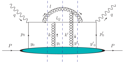
Figure 7:

$${\cal C}_{13}^{c,l,r} = \frac{\alpha_{s}^{2}}{N_{c}}\left[-\frac{C_{A}}{2}\right]\int dl_{\perp}^{2}P(y)\frac{[l_{\perp}\left(l_{\perp}-k_{\perp}\right)+\kappa y^{4}M^{2}]}{[l_{\perp}^{2}+y^{2}M^{2}][\left(l_{\perp}-k_{\perp}\right)^{2}+y^{2}(1-\eta)^{2}M^{2}]}{\bar{I}}_{33}^{c,l,r}$$ (40)

$${\bar{I}}_{13}^{c} = \exp\left[i\left(x_{B}+x_{L}+\frac{x_{M}}{1-y}\right)P^{+}\left({y^{\prime}}_{0}^{-}-{y}_{0}^{-}\right)\right]\exp\left[i\left(\zeta x_{D}+\left(\zeta-1\right)\frac{x_{M}}{1-y}-\zeta\frac{\eta y^{2}}{1-y}x_{L}\right)P^{+}\left({y^{\prime}}_{1}^{-}-{y}_{1}^{-}\right)\right]\theta\left({y}_{0}^{-}-{y}_{1}^{-}\right)$$ (41)

$$\times~{}\theta\left({y^{\prime}}_{0}^{-}-{y^{\prime}}_{1}^{-}\right)\left[1-\exp\left[-i\left(x_{L}+\frac{y}{1-y}x_{M}\right)P^{+}\left({y}_{1}^{-}-{y}_{0}^{-}\right)\right]\right]$$

$$\left[\exp\left\{-i\left(\frac{\zeta}{y(1-\eta)}x_{D}+\frac{\eta(1-y)}{\left(1-\eta\right)}x_{L}+\left(\zeta-1\right)\frac{x_{M}}{1-y}-\zeta\frac{\eta y^{2}}{1-y}x_{L}\right)P^{+}\left({y^{\prime}}_{1}^{-}-{y^{\prime}}_{0}^{-}\right)\right\}\right.$$

$$\left.-\exp\left[i\left(x_{L}+\frac{y}{1-y}x_{M}\right)P^{+}\left({y^{\prime}}_{1}^{-}-{y^{\prime}}_{0}^{-}\right)\right]\right]$$

$${\bar{I}}_{13}^{l} = \exp\left[i\left(x_{B}+x_{L}+\frac{x_{M}}{1-y}\right)P^{+}\left({y^{\prime}}_{0}^{-}-{y}_{0}^{-}\right)\right]\exp\left[i\left(\zeta x_{D}+\left(\zeta-1\right)\frac{x_{M}}{1-y}-\zeta\frac{\eta y^{2}}{1-y}x_{L}\right)P^{+}\left({y^{\prime}}_{1}^{-}-{y}_{1}^{-}\right)\right]\theta\left({y^{\prime}}_{1}^{-}-{y}_{1}^{-}\right)$$ (42)

$$\times~{}\theta\left({y^{\prime}}_{0}^{-}-{y^{\prime}}_{1}^{-}\right)(-1)\left[\exp\left\{-i\left(\frac{\zeta}{y(1-\eta)}x_{D}+\frac{\eta(1-y)}{\left(1-\eta\right)}x_{L}+\left(\zeta-1\right)\frac{x_{M}}{1-y}-\zeta\frac{\eta y^{2}}{1-y}x_{L}\right)P^{+}\left({y^{\prime}}_{1}^{-}-{y^{\prime}}_{0}^{-}\right)\right\}\right.$$

$$\left.-\exp\left[i\left(x_{L}+\frac{y}{1-y}x_{M}\right)P^{+}\left({y^{\prime}}_{1}^{-}-{y^{\prime}}_{0}^{-}\right)\right]\right]$$

$${\bar{I}}_{13}^{r} = \exp\left[i\left(x_{B}+x_{L}+\frac{x_{M}}{1-y}\right)P^{+}\left({y^{\prime}}_{0}^{-}-{y}_{0}^{-}\right)\right]\exp\left[i\left(\zeta x_{D}+\left(\zeta-1\right)\frac{x_{M}}{1-y}-\zeta\frac{\eta y^{2}}{1-y}x_{L}\right)P^{+}\left({y^{\prime}}_{1}^{-}-{y}_{1}^{-}\right)\right]\theta\left({y}_{0}^{-}-{y}_{1}^{-}\right)$$ (43)

$$\times~{}\theta\left({y^{\prime}}_{1}^{-}-{y}_{1}^{-}\right)\left[\exp\left\{i\left(\frac{\zeta}{y(1-\eta)}x_{D}+\frac{\eta(1-y)}{\left(1-\eta\right)}x_{L}+\left(\zeta-1\right)\frac{x_{M}}{1-y}-\zeta\frac{\eta y^{2}}{1-y}x_{L}\right)P^{+}\left(y_{1}^{-}-y_{0}^{-}\right)\right\}\right.$$

$$\left.-\exp\left[-i\left(x_{L}+\frac{y}{1-y}x_{M}\right)P^{+}\left({y}_{1}^{-}-{y}_{0}^{-}\right)\right]\right]\left[-\exp\left\{-i\left(\frac{-\zeta(1-2y(1-\eta))}{y(1-\eta)}x_{D}-\frac{\eta(1-y)}{\left(1-\eta\right)}x_{L}+\left(\zeta-1\right)\frac{x_{M}}{1-y}\right.\right.\right.$$

$$\left.\left.\left.-\zeta\frac{\eta y^{2}}{1-y}x_{L}\right)P^{+}\left({y^{\prime}}_{1}^{-}-{y}_{1}^{-}\right)\right\}\right]$$

The contributions from the three cuts in Fig.[8] are,

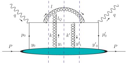
Figure 8:

$${\cal C}_{31}^{c,l,r} = \frac{\alpha_{s}^{2}}{N_{c}}\left[-\frac{C_{A}}{2}\right]\int dl_{\perp}^{2}P(y)\frac{[\left(l_{\perp}-k_{\perp}\right)l_{\perp}+\kappa y^{4}M^{2}]}{[\left(l_{\perp}-k_{\perp}\right)^{2}+y^{2}(1-\eta)^{2}M^{2}][l_{\perp}^{2}+y^{2}M^{2}]}{\bar{I}}_{31}^{c,l,r}$$

$${\bar{I}}_{31}^{c} = \exp\left[i\left(x_{B}+x_{L}+\frac{x_{M}}{1-y}\right)P^{+}\left({y^{\prime}}_{0}^{-}-{y}_{0}^{-}\right)\right]\exp\left[i\left(\zeta x_{D}+\left(\zeta-1\right)\frac{x_{M}}{1-y}-\zeta\frac{\eta y^{2}}{1-y}x_{L}\right)P^{+}\left({y^{\prime}}_{1}^{-}-{y}_{1}^{-}\right)\right]\theta\left({y}_{0}^{-}-{y}_{1}^{-}\right)$$ (44)

$$\times~{}\theta\left({y^{\prime}}_{0}^{-}-{y^{\prime}}_{1}^{-}\right)\left[\exp\left\{i\left(\frac{\zeta}{y(1-\eta)}x_{D}+\frac{\eta(1-y)}{\left(1-\eta\right)}x_{L}+\left(\zeta-1\right)\frac{x_{M}}{1-y}-\zeta\frac{\eta y^{2}}{1-y}x_{L}\right)P^{+}\left({y}_{1}^{-}-{y}_{0}^{-}\right)\right\}\right.$$

$$\left.-\exp\left[-i\left(x_{L}+\frac{y}{1-y}x_{M}\right)P^{+}\left({y}_{1}^{-}-{y}_{0}^{-}\right)\right]\right]\left[1-\exp\left[i\left(x_{L}+\frac{y}{1-y}x_{M}\right)P^{+}\left({y^{\prime}}_{1}^{-}-{y^{\prime}}_{0}^{-}\right)\right]\right]$$

$${\bar{I}}_{31}^{l} = \exp\left[i\left(x_{B}+x_{L}+\frac{x_{M}}{1-y}\right)P^{+}\left({y^{\prime}}_{0}^{-}-{y}_{0}^{-}\right)\right]\exp\left[i\left(\zeta x_{D}+\left(\zeta-1\right)\frac{x_{M}}{1-y}-\zeta\frac{\eta y^{2}}{1-y}x_{L}\right)P^{+}\left({y^{\prime}}_{1}^{-}-{y}_{1}^{-}\right)\right]\theta\left({y^{\prime}}_{0}^{-}-{y^{\prime}}_{1}^{-}\right)$$ (45)

$$\times~{}\theta\left({y^{\prime}}_{1}^{-}-{y}_{1}^{-}\right)\left[-\exp\left\{-i\left(\frac{-\zeta(1-2y(1-\eta))}{y(1-\eta)}x_{D}-\frac{\eta(1-y)}{\left(1-\eta\right)}x_{L}+\left(\zeta-1\right)\frac{x_{M}}{1-y}-\zeta\frac{\eta y^{2}}{1-y}x_{L}\right)P^{+}\left({y^{\prime}}_{1}^{-}-{y}_{1}^{-}\right)\right\}\right]$$

$$\left[\exp\left\{-i\left(\frac{\zeta}{y(1-\eta)}x_{D}+\frac{\eta(1-y)}{\left(1-\eta\right)}x_{L}+\left(\zeta-1\right)\frac{x_{M}}{1-y}-\zeta\frac{\eta y^{2}}{1-y}x_{L}\right)P^{+}\left({y^{\prime}}_{1}^{-}-{y^{\prime}}_{0}^{-}\right)\right\}\right.$$

$$\left.-\exp\left[i\left(x_{L}+\frac{y}{1-y}x_{M}\right)P^{+}\left({y^{\prime}}_{1}^{-}-{y^{\prime}}_{0}^{-}\right)\right]\right]$$

$${\bar{I}}_{31}^{r} = \exp\left[i\left(x_{B}+x_{L}+\frac{x_{M}}{1-y}\right)P^{+}\left({y^{\prime}}_{0}^{-}-{y}_{0}^{-}\right)\right]\exp\left[i\left(\zeta x_{D}+\left(\zeta-1\right)\frac{x_{M}}{1-y}-\zeta\frac{\eta y^{2}}{1-y}x_{L}\right)P^{+}\left({y^{\prime}}_{1}^{-}-{y}_{1}^{-}\right)\right]\theta\left({y}_{1}^{-}-{y^{\prime}}_{1}^{-}\right)$$ (46)

$$\times~{}\theta\left({y}_{0}^{-}-{y}_{1}^{-}\right)(-1)\left[\exp\left\{i\left(\frac{\zeta}{y(1-\eta)}x_{D}+\frac{\eta(1-y)}{\left(1-\eta\right)}x_{L}+\left(\zeta-1\right)\frac{x_{M}}{1-y}-\zeta\frac{\eta y^{2}}{1-y}x_{L}\right)P^{+}\left({y}_{1}^{-}-{y}_{0}^{-}\right)\right\}\right.$$

$$\left.-\exp\left[-i\left(x_{L}+\frac{y}{1-y}x_{M}\right)P^{+}\left({y}_{1}^{-}-{y}_{0}^{-}\right)\right]\right]$$

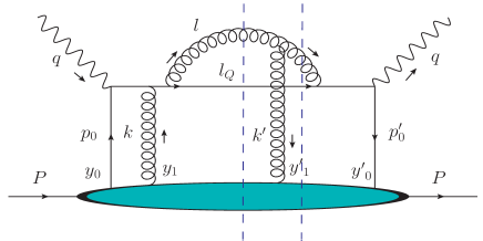
Figure 9:

Contributions from two cuts from Fig.[9] are as follows,

$${\cal C}_{23}^{c} = \frac{\alpha_{s}^{2}}{N_{c}}\left[-\frac{C_{A}}{2}\right]\int dl_{\perp}^{2}\left(\frac{1+(1-y)^{2}}{y}\right)\frac{[\left(l_{\perp}-yk_{\perp}\right)\left(l_{\perp}-k_{\perp}\right)+\kappa y^{4}M^{2}]}{\left[\left(l_{\perp}-yk_{\perp}\right)^{2}+y^{2}M^{2}+2y\left(\frac{k^{-}}{l^{-}}\right)l_{\perp}^{2}\right][\left(l_{\perp}-k_{\perp}\right)^{2}+y^{2}(1-\eta)^{2}M^{2}]}{\bar{I}}_{23}^{c}$$

$${\bar{I}}_{23}^{c} = \exp\left[i\left(x_{B}+x_{L}+\frac{x_{M}}{1-y}\right)P^{+}\left({y^{\prime}}_{0}^{-}-{y}_{0}^{-}\right)\right]\exp\left[i\left(\zeta x_{D}+\left(\zeta-1\right)\frac{x_{M}}{1-y}-\zeta\frac{\eta y^{2}}{1-y}x_{L}\right)P^{+}\left({y^{\prime}}_{1}^{-}-{y}_{1}^{-}\right)\right]$$ (47)

$$\theta\left({y}_{0}^{-}-{y}_{1}^{-}\right)\theta\left({y^{\prime}}_{0}^{-}-{y^{\prime}}_{1}^{-}\right)\left[-\exp\left[-i\left(x_{L}+\frac{y}{1-y}x_{M}\right)P^{+}\left({y}_{1}^{-}-{y}_{0}^{-}\right)\right]\right]$$

$$\left[\exp\left\{-i\left(\frac{\zeta}{y(1-\eta)}x_{D}+\frac{\eta(1-y)}{\left(1-\eta\right)}x_{L}+\left(\zeta-1\right)\frac{x_{M}}{1-y}-\zeta\frac{\eta y^{2}}{1-y}x_{L}\right)\right.\right.$$

$$\left.\left.\times~{}P^{+}\left({y^{\prime}}_{1}^{-}-{y^{\prime}}_{0}^{-}\right)\right\}-\exp\left[i\left(x_{L}+\frac{y}{1-y}x_{M}\right)P^{+}\left({y^{\prime}}_{1}^{-}-{y^{\prime}}_{0}^{-}\right)\right]\right]$$

$${\cal C}_{23}^{r} = \frac{\alpha_{s}^{2}}{N_{c}}\left[-\frac{C_{A}}{2}\right]\int dl_{\perp}^{2}\left(\frac{1+(1-y)^{2}}{y}\right)\frac{[l_{\perp}\left(l_{\perp}-(1-y)k_{\perp}\right)+\kappa y^{4}M^{2}]}{\left[l_{\perp}^{2}+y^{2}M^{2}\right][\left(l_{\perp}-(1-y)k_{\perp}\right)^{2}+y^{2}(1-\eta)^{2}M^{2}]}{\bar{I}}_{23}^{r}$$ (48)

$${\bar{I}}_{23}^{r} = \exp\left[i\left(x_{B}+x_{L}+\frac{x_{M}}{1-y}\right)P^{+}\left({y^{\prime}}_{0}^{-}-{y}_{0}^{-}\right)\right]\exp\left[i\left(\zeta x_{D}+\left(\zeta-1\right)\frac{x_{M}}{1-y}-\zeta\frac{\eta y^{2}}{1-y}x_{L}\right)P^{+}\left({y^{\prime}}_{1}^{-}-{y}_{1}^{-}\right)\right]$$ (49)

$$\times~{}\theta\left({y}_{1}^{-}-{y^{\prime}}_{1}^{-}\right)\theta\left({y}_{0}^{-}-{y}_{1}^{-}\right)\left[\exp\left[-i\left(x_{L}+\frac{y}{1-y}x_{M}\right)P^{+}\left({y^{\prime}}_{1}^{-}-{y}_{0}^{-}\right)-i\left(x_{K}-x_{D}\right)P^{+}\left({y}_{1}^{-}-{y^{\prime}}_{1}^{-}\right)\right]\right.$$

$$\left.-\exp\left[-i\left(\frac{-\zeta(1-2y(1-\eta))}{y(1-\eta)}x_{D}-\frac{\eta(1-y)}{\left(1-\eta\right)}x_{L}\right)P^{+}\left({y^{\prime}}_{1}^{-}-{y}_{1}^{-}\right)-i\left(x_{L}+\frac{y}{1-y}x_{M}\right)P^{+}\left({y}_{1}^{-}-{y}_{0}^{-}\right)\right]\right]$$

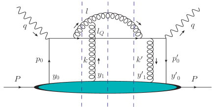
Figure 10:

Contributions of Fig.[10] are,

$${\cal C}_{32}^{c} = \frac{\alpha_{s}^{2}}{N_{c}}\left[\frac{C_{A}}{2}\right]\int dl_{\perp}^{2}\left(\frac{1+(1-y)^{2}}{y}\right)\frac{[\left(l_{\perp}-k_{\perp}\right)\left(l_{\perp}-yk_{\perp}\right)+\kappa y^{4}M^{2}]}{[\left(l_{\perp}-k_{\perp}\right)^{2}+y^{2}(1-k^{-}/l^{-})^{2}M^{2}]\left[\left(l_{\perp}-yk_{\perp}\right)^{2}+y^{2}M^{2}+2y\left(\frac{k^{-}}{l^{-}}\right)l_{\perp}^{2}\right]}{\bar{I}}_{32}^{c}$$

$${\bar{I}}_{32}^{c} = \exp\left[i\left(x_{B}+x_{L}+\frac{x_{M}}{1-y}\right)P^{+}\left({y^{\prime}}_{0}^{-}-{y}_{0}^{-}\right)\right]\exp\left[i\left(\zeta x_{D}+\left(\zeta-1\right)\frac{x_{M}}{1-y}-\zeta\frac{\eta y^{2}}{1-y}x_{L}\right)P^{+}\left({y^{\prime}}_{1}^{-}-{y}_{1}^{-}\right)\right]\theta\left({y}_{0}^{-}-{y}_{1}^{-}\right)$$ (51)

$$\times~{}\theta\left({y^{\prime}}_{0}^{-}-{y^{\prime}}_{1}^{-}\right)\left[\exp\left\{i\left(\frac{\zeta}{y(1-\eta)}x_{D}+\frac{\eta(1-y)}{\left(1-\eta\right)}x_{L}+\left(\zeta-1\right)\frac{x_{M}}{1-y}-\zeta\frac{\eta y^{2}}{1-y}x_{L}\right)P^{+}\left(y_{1}^{-}-y_{0}^{-}\right)\right\}\right.$$

$$\left.-\exp\left[-i\left(x_{L}+\frac{y}{1-y}x_{M}\right)P^{+}\left({y}_{1}^{-}-{y}_{0}^{-}\right)\right]\right]\left[-\exp\left[i\left(x_{L}+\frac{y}{1-y}x_{M}\right)P^{+}\left({y^{\prime}}_{1}^{-}-{y^{\prime}}_{0}^{-}\right)\right]\right]$$

$${\cal C}_{32}^{l} = \frac{\alpha_{s}^{2}}{N_{c}}\left[\frac{C_{A}}{2}\right]\int dl_{\perp}^{2}\left(\frac{1+(1-y)^{2}}{y}\right)\frac{[\left(l_{\perp}-(1-y)k_{\perp}\right)l_{\perp}+\kappa y^{4}M^{2}]}{[\left(l_{\perp}-k_{\perp}\right)^{2}+y^{2}(1-\eta)^{2}M^{2}]\left[\left(l_{\perp}-yk_{\perp}\right)^{2}+y^{2}M^{2}+2y\eta l_{\perp}^{2}\right]}{\bar{I}}_{32}^{l}$$

$${\bar{I}}_{12}^{l} = \exp\left[i\left(x_{B}+x_{L}+\frac{x_{M}}{1-y}\right)P^{+}\left({y^{\prime}}_{0}^{-}-{y}_{0}^{-}\right)\right]\exp\left[i\left(\zeta x_{D}+\left(\zeta-1\right)\frac{x_{M}}{1-y}-\zeta\frac{\eta y^{2}}{1-y}x_{L}\right)P^{+}\left({y^{\prime}}_{1}^{-}-{y}_{1}^{-}\right)\right]$$ (53)

$$\times~{}\theta\left({y^{\prime}}_{1}^{-}-{y}_{1}^{-}\right)\theta\left({y^{\prime}}_{0}^{-}-{y^{\prime}}_{1}^{-}\right)(-1)\left[\exp\left[i\left(x_{L}+\frac{y}{1-y}x_{M}\right)P^{+}\left({y}_{1}^{-}-{y^{\prime}}_{0}^{-}\right)+i\left(x_{K}-x_{D}\right)P^{+}\left({y^{\prime}}_{1}^{-}-y_{1}^{-}\right)\right]\right.$$

$$\left.-\exp\left[i\left(\frac{-\zeta(1-2y(1-\eta))}{y(1-\eta)}x_{D}-\frac{\eta(1-y)}{\left(1-\eta\right)}x_{L}\right)P^{+}\left({y}_{1}^{-}-{y^{\prime}}_{1}^{-}\right)+i\left(x_{L}+\frac{y}{1-y}x_{M}\right)P^{+}\left({y^{\prime}}_{1}^{-}-{y^{\prime}}_{0}^{-}\right)\right]\right]$$

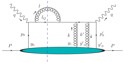
Figure 11:

Fig.[11] has one possible cut,

$${\cal C}_{10}^{l} = \frac{\alpha_{s}^{2}}{N_{c}}\left[C_{F}\right]\int dl_{\perp}^{2}P(y)\frac{[l_{\perp}^{2}+\kappa y^{4}M^{2}]}{(l_{\perp}^{2}+y^{2}M^{2})^{2}}~{}{\bar{I}}_{10}^{l}$$ (54)

$${\bar{I}}_{10}^{l} = \exp\left[i\left(x_{B}+x_{L}+\frac{x_{M}}{1-y}\right)P^{+}\left({y^{\prime}}_{0}^{-}-{y}_{0}^{-}\right)\right]\exp\left[i\left(\zeta x_{D}+\left(\zeta-1\right)\frac{x_{M}}{1-y}-\zeta\frac{\eta y^{2}}{1-y}x_{L}\right)P^{+}\left({y^{\prime}}_{1}^{-}-{y}_{1}^{-}\right)\right]\theta\left({y^{\prime}}_{1}^{-}-{y}_{1}^{-}\right)$$ (55)

$$\times~{}\theta\left({y^{\prime}}_{0}^{-}-{y^{\prime}}_{1}^{-}\right)\left[-\exp\left[-i\left(x_{K}-x_{D}\right)P^{+}\left({y^{\prime}}_{1}^{-}-y_{1}^{-}\right)\right]\exp\left[i\left(x_{L}+\frac{y}{1-y}x_{M}\right)P^{+}\left({y}_{1}^{-}-{y^{\prime}}_{0}^{-}\right)\right]\right]$$

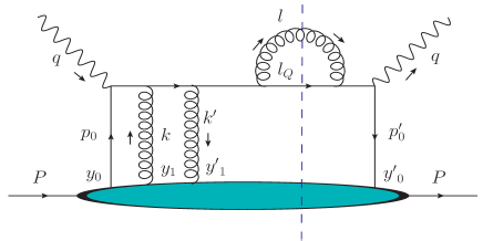
Figure 12:

Fig.[12] also has single possible cut,

$${\cal C}_{01}^{l} = \frac{\alpha_{s}^{2}}{N_{c}}\left[C_{F}\right]\int dl_{\perp}^{2}P(y)\frac{[l_{\perp}^{2}+\kappa y^{4}M^{2}]}{(l_{\perp}^{2}+y^{2}M^{2})^{2}}~{}{\bar{I}}_{10}^{l}$$ (56)

$${\bar{I}}_{01}^{r} = \exp\left[i\left(x_{B}+x_{L}+\frac{x_{M}}{1-y}\right)P^{+}\left({y^{\prime}}_{0}^{-}-{y}_{0}^{-}\right)\right]\exp\left[i\left(\zeta x_{D}+\left(\zeta-1\right)\frac{x_{M}}{1-y}-\zeta\frac{\eta y^{2}}{1-y}x_{L}\right)P^{+}\left({y^{\prime}}_{1}^{-}-{y}_{1}^{-}\right)\right]\theta\left({y^{\prime}}_{1}^{-}-{y}_{1}^{-}\right)$$ (57)

$$\times~{}\theta\left({y^{\prime}}_{0}^{-}-{y^{\prime}}_{1}^{-}\right)\left[-\exp\left[i\left(x_{K}-x_{D}\right)P^{+}\left({y^{\prime}}_{1}^{-}-{y}_{1}^{-}\right)\right]\exp\left[-i\left(x_{L}+\frac{y}{1-y}x_{M}\right)P^{+}\left({y^{\prime}}_{1}^{-}-{y}_{0}^{-}\right)\right]\right]$$

References

• (1) X. N. Wang and M. Gyulassy, Phys. Rev. Lett.  68, 1480 (1992).
• (2) M. Gyulassy and X. n. Wang, Nucl. Phys. B 420, 583 (1994) [nucl-th/9306003].
• (3) R. Baier, Y. L. Dokshitzer, A. H. Mueller, S. Peigne and D. Schiff, Nucl. Phys. B 483, 291 (1997) [hep-ph/9607355].
• (4) B. G. Zakharov, JETP Lett.  63, 952 (1996) [hep-ph/9607440].
• (5) A. Majumder and M. Van Leeuwen, Prog. Part. Nucl. Phys. A 66, 41 (2011) [arXiv:1002.2206 [hep-ph]].
• (6) U. A. Wiedemann, Landolt-Bornstein 23, 521 (2010) [arXiv:0908.2306 [hep-ph]].
• (7) N. Armesto, B. Cole, C. Gale, W. A. Horowitz, P. Jacobs, S. Jeon, M. van Leeuwen and A. Majumder et al., Phys. Rev. C 86 (2012) 064904 [arXiv:1106.1106 [hep-ph]].
• (8) G. Y. Qin and A. Majumder, Phys. Rev. Lett.  105, 262301 (2010) [arXiv:0910.3016 [hep-ph]].
• (9) M. Djordjevic, Phys. Rev. Lett.  112, no. 4, 042302 (2014) [arXiv:1307.4702 [nucl-th]].
• (10) B. I. Abelev et al. [STAR Collaboration], Phys. Rev. Lett.  98, 192301 (2007) [Phys. Rev. Lett.  106, 159902 (2011)] [nucl-ex/0607012].
• (11) A. Adare et al. [PHENIX Collaboration], Phys. Rev. Lett.  98, 172301 (2007) [nucl-ex/0611018].
• (12) M. Djordjevic and M. Gyulassy, Nucl. Phys. A 733, 265 (2004) [nucl-th/0310076].
• (13) M. Djordjevic, M. Gyulassy and S. Wicks, Phys. Rev. Lett.  94, 112301 (2005) [hep-ph/0410372].
• (14) B. Abelev et al. [ALICE Collaboration], JHEP 1209, 112 (2012) [arXiv:1203.2160 [nucl-ex]].
• (15) K. Aamodt et al. [ALICE Collaboration], Phys. Lett. B 696, 30 (2011) [arXiv:1012.1004 [nucl-ex]].
• (16) M. G. Mustafa, Phys. Rev. C 72, 014905 (2005) [hep-ph/0412402].
• (17) S. Wicks, W. Horowitz, M. Djordjevic and M. Gyulassy, Nucl. Phys. A 784, 426 (2007) [nucl-th/0512076].
• (18) R. Abir, C. Greiner, M. Martinez, M. G. Mustafa and J. Uphoff, Phys. Rev. D 85, 054012 (2012) [arXiv:1109.5539 [hep-ph]].
• (19) R. Abir, U. Jamil, M. G. Mustafa and D. K. Srivastava, Phys. Lett. B 715, 183 (2012) [arXiv:1203.5221 [hep-ph]].
• (20) B. W. Zhang, E. k. Wang and X. N. Wang, Nucl. Phys. A 757, 493 (2005) [hep-ph/0412060].
• (21) M. He, R. J. Fries and R. Rapp, Nucl. Phys. A 910-911, 409 (2013) [arXiv:1208.0256 [nucl-th]].
• (22) S. Cao and S. A. Bass, Phys. Rev. C 84, 064902 (2011) [arXiv:1108.5101 [nucl-th]].
• (23) G. D. Moore and D. Teaney, Phys. Rev. C 71, 064904 (2005) [hep-ph/0412346].
• (24) R. Baier, Nucl. Phys. A 715, 209 (2003) [hep-ph/0209038].
• (25) A. Majumder, Phys. Rev. C 87, 034905 (2013) [arXiv:1202.5295 [nucl-th]].
• (26) A. Majumder, Phys. Rev. C 80, 031902 (2009) [arXiv:0810.4967 [nucl-th]].
• (27) G. Y. Qin and A. Majumder, arXiv:1411.5642 [nucl-th].
• (28) C. W. Bauer, S. Fleming, D. Pirjol and I. W. Stewart, Phys. Rev. D 63, 114020 (2001) [hep-ph/0011336].
• (29) C. W. Bauer and I. W. Stewart, Phys. Lett. B 516, 134 (2001) [hep-ph/0107001].
• (30) C. W. Bauer, D. Pirjol and I. W. Stewart, Phys. Rev. D 65, 054022 (2002) [hep-ph/0109045].
• (31) C. W. Bauer, S. Fleming, D. Pirjol, I. Z. Rothstein and I. W. Stewart, Phys. Rev. D 66, 014017 (2002) [hep-ph/0202088].
• (32) R. Abir, G. D. Kaur and A. Majumder, arXiv:1407.1864 [nucl-th].
• (33) A. Idilbi and A. Majumder, Phys. Rev. D 80, 054022 (2009) [arXiv:0808.1087 [hep-ph]].
• (34) F. D’Eramo, H. Liu and K. Rajagopal, Phys. Rev. D 84, 065015 (2011) [arXiv:1006.1367 [hep-ph]].
• (35) G. -Y. Qin and A. Majumder, Phys. Rev. C 87, 024909 (2013) [arXiv:1205.5741 [hep-ph]].
• (36) Y. L. Dokshitzer and D. E. Kharzeev, Phys. Lett. B 519, 199 (2001) [hep-ph/0106202].
• (37) X. N. Wang and X. f. Guo, Nucl. Phys. A 696, 788 (2001) [hep-ph/0102230].
• (38) L. D. Landau and I. Pomeranchuk, Dokl. Akad. Nauk Ser. Fiz.  92, 535 (1953).
• (39) A. B. Migdal, Phys. Rev.  103, 1811 (1956).
• (40) A. Majumder, Phys. Rev. D 85, 014023 (2012) [arXiv:0912.2987 [nucl-th]].