Dyadic data analysis with amen

Abstract

Dyadic data on pairs of objects, such as relational or social network data, often exhibit strong statistical dependencies. Certain types of second-order dependencies, such as degree heterogeneity and reciprocity, can be well-represented with additive random effects models. Higher-order dependencies, such as transitivity and stochastic equivalence, can often be represented with multiplicative effects. The amen package for the R statistical computing environment provides estimation and inference for a class of additive and multiplicative random effects models for ordinal, continuous, binary and other types of dyadic data. The package also provides methods for missing, censored and fixed-rank nomination data, as well as longitudinal dyadic data. This tutorial illustrates the amen package via example statistical analyses of several of these different data types.

Keywords: Bayesian estimation, dyadic data, latent factor model, MCMC, random effects, regression, relational data, social network.

1 The Gaussian AME model

A pair of objects, individuals or nodes is called a dyad, and a variable that is measured or observed on multiple dyads is called a dyadic variable. Data on such a variable may be referred to as dyadic data, relational data, or network data (particularly if the variable is binary). Dyadic data for a population of $n$ objects, individuals or nodes may be represented as a sociomatrix, an $n\times n$ square matrix ${\mathbf{Y}}$ with an undefined diagonal. The $i,j$th entry of ${\mathbf{Y}}$, denoted $y_{i,j}$, gives the value of the variable for dyad $\{i,j\}$ from the perspective of node $i$, or in the direction from $i$ to $j$. For example, in a dataset describing friendship relations, $y_{i,j}$ might represent a quantification of how much person $i$ likes person $j$. A running example in this section will be an analysis of international trade data, where $y_{i,j}$ is the (log) dollar-value of exports from country $i$ to country $j$. These data can be obtained from the IR90s dataset included in the amen package. Specifically, we will analyze trade data between the 30 countries having the highest GDPs:

#### —- obtain trade data from top 30 countries in terms of GDP
data(IR90s)

gdp<-IR90s$nodevars[,2]
topgdp<-which(gdp>=sort(gdp,decreasing=TRUE)[30] )
Y<-log( IR90s$dyadvars[topgdp,topgdp,2] + 1 )

Y[1:5,1:5]

          ARG        AUL       BEL        BNG        BRA
ARG        NA 0.05826891 0.2468601 0.03922071 1.76473080
AUL 0.0861777         NA 0.3784364 0.10436002 0.21511138
BEL 0.2700271 0.35065687        NA 0.01980263 0.39877612
BNG 0.0000000 0.01980263 0.1222176         NA 0.01980263
BRA 1.6937791 0.23901690 0.6205765 0.03922071         NA

1.1 The social relations model

Dyadic data often exhibit certain types of statistical dependencies. For example, it is often the case that observations in a given row of the sociomatrix are similar to or correlated with each other. This should not be too surprising, as these observations all share a common “sender,” or row index. If a sender $i_{1}$ is more “sociable” than sender $i_{2}$, we would expect the values in row $i_{1}$ to be larger than those in row $i_{2}$, on average. In this way, heterogeneity of the nodes in terms of their “sociability” corresponds to a large variance of the row means of the sociomatrix. Similarly, nodal heterogeneity in “popularity” corresponds to a large variance in the column means.

A classical approach to evaluating across-row and across-column heterogeneity in a data matrix is the ANOVA decomposition. A model-based version of the ANOVA decomposition posits that the variability of the $y_{i,j}$’s around some overall mean is well-represented by additive row and column effects:

$$y_{i,j}=\mu+a_{i}+b_{j}+\epsilon_{i,j}.$$

In this model, heterogeneity among the parameters $\{a_{i}:i=1,\ldots,n\}$ and $\{b_{j}:j=1,\ldots,n\}$ corresponds to observed heterogeneity in the row means and column means of the sociomatrix, respectively. If the $\epsilon_{i,j}$’s are assumed to be i.i.d. from a mean-zero normal distribution, the hypothesis of no row heterogeneity (all $a_{i}$’s equal to zero) or no column heterogeneity (all $b_{j}$’s equal to zero) can be evaluated with normal-theory $F$-tests. For the trade data, this can be done in R as follows:

#### —- ANOVA for trade data

Rowcountry<-matrix(rownames(Y),nrow(Y),ncol(Y))
Colcountry<-t(Rowcountry)

anova(lm( c(Y) ~ c(Rowcountry) + c(Colcountry) ) )

Analysis of Variance Table

Response: c(Y)
               Df Sum Sq Mean Sq F value    Pr(>F)
c(Rowcountry)  29 202.48  6.9819  29.524 < 2.2e-16 ***
c(Colcountry)  29 206.32  7.1144  30.084 < 2.2e-16 ***
Residuals     811 191.79  0.2365
---
Signif. codes:  0 ’***’ 0.001 ’**’ 0.01 ’*’ 0.05 ’.’ 0.1 ’ ’ 1

The results indicate a large degree of heterogeneity of the countries as both exporters and importers - much more than would be expected if the “true” $a_{i}$’s were all zero, or the “true” $b_{j}$’s were all zero (and the $\epsilon_{i,j}$’s were i.i.d.). Based on this result, the next steps in a data analysis might include comparisons of the row means or of the column means, that is, comparisons of the countries in terms of their total or average imports and exports. This can equivalently be done via comparisons among estimates of the row and column effects:

#### —- comparison of countries in terms of row and column means
rmean<-rowMeans(Y,na.rm=TRUE) ; cmean<-colMeans(Y,na.rm=TRUE)

muhat<-mean(Y,na.rm=TRUE)
ahat<-rmean-muhat
bhat<-cmean-muhat

# additive ”exporter” effects
head( sort(ahat,decreasing=TRUE)  )

      USA       JPN       UKG       FRN       ITA       CHN
1.4801300 1.0478834 0.6140597 0.5919777 0.4839285 0.4468015

# additive ”importer” effects
head( sort(bhat,decreasing=TRUE)  )

      USA       JPN       UKG       FRN       ITA       NTH
1.5628243 0.8433793 0.6683700 0.5849702 0.4712668 0.3628532

We note that these simple estimates here are very close to, but not exactly the same as, the least squares/maximum likelihood estimates (this is because of the undefined diagonal in the sociomatrix).

While straightforward to implement, this classical ANOVA analysis ignores a fundamental characteristic of dyadic data: Each node appears in the dataset as both a sender and a receiver of relations, or equivalently, the row and column labels of the data matrix refer to the same set of objects. In the context of the ANOVA model, this means that each node $i$ has two additive effects: a row effect $a_{i}$ and a column effect $b_{i}$. Often it is of interest to evaluate the extent to which these effects are correlated, for example, to evaluate if sociable nodes in the network are also popular. Additionally, each (unordered) pair of nodes $i,j$ has two outcomes, $y_{i,j}$ and $y_{j,i}$. It is often the case that $y_{i,j}$ and $y_{j,i}$ are correlated, as these two observations come from the same dyad.

Correlations between the additive effects can be evaluated empirically simply by computing the sample covariance of the row means and column means, or alternatively, the $\hat{a}_{i}$’s and $\hat{b}_{i}$’s. Dyadic correlation can be evaluated by computing the correlation between the matrix of residuals from the ANOVA model and its transpose:

#### —- covariance and correlation between row and column effects
cov( cbind(ahat,bhat) )

          ahat      bhat
ahat 0.2407563 0.2290788
bhat 0.2290788 0.2289489

cor( ahat, bhat)

[1] 0.9757237

#### —- an estimate of dyadic covariance and correlation
R <- Y - ( muhat + outer(ahat,bhat,"+") )
cov( cbind( c(R),c(t(R)) ), use="complete")

          [,1]      [,2]
[1,] 0.2212591 0.1900891
[2,] 0.1900891 0.2212591

cor( c(R),c(t(R)), use="complete")

[1] 0.8591242

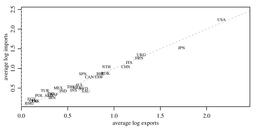
Figure 1: Scatterplot of country-level average imports versus exports.

As shown by these calculations and in Figure 1, country-level export and import volumes are highly correlated, as are the export and import volumes within country pairs. A seminal model for analyzing such within-node and within-dyad dependence is the social relations model, or SRM (Warner et al., 1979), a type of ANOVA decomposition that describes variability among the entries of the sociomatrix ${\mathbf{Y}}$ in terms of within-row, within-column and within-dyad variability. A normal random-effects version of the SRM has been studied by Wong (1982) and Li and Loken (2002), among others, and takes the following form:

$$y_{i,j} =\mu+a_{i}+b_{j}+\epsilon_{i,j}$$ (1)

$$\{(a_{1},b_{1}),\ldots,(a_{n},b_{n})\} \sim\text{i.i.d.}\ N(0,\Sigma_{ab})$$

$$\{(\epsilon_{i,j},\epsilon_{j,i}):i\neq j\} \sim\text{i.i.d.}\ N(0,\Sigma_{e}),$$

where

$$\Sigma_{ab}=\begin{pmatrix}\sigma^{2}_{a}&\sigma_{ab}\\ \sigma_{ab}&\sigma_{b}^{2}\end{pmatrix}\ \ \text{and}\ \ \Sigma_{\epsilon}=\sigma^{2}_{\epsilon}\begin{pmatrix}1&\rho\\ \rho&1\end{pmatrix}.$$

Note that conditional on the row effects $\{a_{1},\ldots,a_{n}\}$, the mean in the $i$th row of ${\mathbf{Y}}$ is given by $\mu+a_{i}$, and the variability of these row-specific means is given by $\sigma^{2}_{a}$. In this way, the row effects represent across-row heterogeneity in the sociomatrix, and $\sigma_{a}^{2}$ is a single-number summary of this heterogeneity. Similarly, the column effects $\{b_{1},\ldots,b_{n}\}$ represent heterogeneity in the column means, and $\sigma^{2}_{b}$ summarizes this heterogeneity. The covariance $\sigma_{ab}$ describes the linear association between these row and column effects, or equivalently, the association between the row means and column means of the sociomatrix. Additional variability across dyads is described by $\sigma^{2}_{\epsilon}$, and within dyad correlation (beyond that described by $\sigma_{ab}$) is captured by $\rho$. More precisely, straightforward calculations show that under this random effects model,

$${\text{Var}}[y_{i,j}] =\sigma^{2}_{a}+2\sigma_{ab}+\sigma^{2}_{b}+\sigma_{\epsilon}^{2}$$ (across-dyad variance) (2)

$${\text{Cov}}[y_{i,j},y_{i,k}] =\sigma_{a}^{2}$$ (within-row covariance)

$${\text{Cov}}[y_{i,j},y_{k,j}] =\sigma_{b}^{2}$$ (within-column covariance)

$${\text{Cov}}[y_{i,j},y_{j,k}] =\sigma_{ab}$$ (row-column covariance)

$${\text{Cov}}[y_{i,j},y_{j,i}] =2\sigma_{ab}+\rho\sigma^{2}_{e} \text{(row-column covariance plus reciprocity) },$$

with all other covariances between elements of ${\mathbf{Y}}$ being zero. We refer to this covariance model as the social relations covariance model.

The amen package provides model fitting and evaluation tools for the SRM via the default values of the ame command:

fit_SRM<-ame(Y)

Figure 2: Default plots generated by the ame command.

Running this command initiates an iterative Markov chain Monte Carlo (MCMC) algorithm that provides Bayesian inference for the parameters in the SRM model. The progress of the algorithm is displayed via a sequence of plots, the last of which is shown in Figure 2. The top row gives traceplots of the parameter values simulated from their posterior distribution, including covariance parameters on the left and regression parameters on the right. The covariance parameters include $\Sigma_{ab}$, $\rho$, and $\sigma^{2}$, and are stored as the list component VC in the fitted object. The only regression parameter for this SRM model is the intercept $\mu$, which is included by default for the Gaussian SRM. The intercept, and any other regression parameters are stored as BETA in the fitted object. We can compare these estimates obtained from amen to the estimates from the ANOVA-style approach as follows:

muhat                                # empirical overall mean  

[1] 0.680044

mean(fit_SRM$BETA)                   # model-based estimate

[1] 0.6616449

cov( cbind(ahat,bhat) )              # empirical row/column mean covariance 

          ahat      bhat
ahat 0.2407563 0.2290788
bhat 0.2290788 0.2289489

apply(fit_SRM$VC[,1:3],2,mean)       # model-based estimate    

       va       cab        vb
0.2811301 0.2368096 0.2728049

cor( c(R), c(t(R)) , use="complete") # empirical residual dyadic correlation

[1] 0.8591242

mean(fit_SRM$VC[,4])                 # model-based estimate

[1] 0.857584

Posterior mean estimates of the row and column effects can be accessed from fit_SRM$APM and fit_SRM$BPM, respectively. These estimates are plotted in Figure 3, against the corresponding ANOVA estimates.

Figure 3: Bayes versus least squares parameter estimates.

The second two rows of Figure 2 give posterior predictive goodness of fit summaries for four network statistics: (1) the empirical standard deviation of the row means; (2) the empirical standard deviation of the column means; (3) the empirical within-dyad correlation; (4) a normalized measure of triadic dependence. Details on how these are computed can be obtained by examining the gofstats function of the amen package. The blue histograms in the figure represent values of gofstats(Ysim), where Ysim is simulated from the posterior predictive distribution. These histograms should be compared to the observed statistics gofstats(Y), which for these data are 0.491, 0.478, 0.939 and 0.204, given by vertical red lines in the figure. Generally speaking, large discrepancies between the posterior predictive distributions (histograms) and the observed statistics (red lines) suggest model lack of fit. For these data, the model does well at representing the data with respect to the first three statistics, but shows a discrepancy with regard to the triadic dependence statistic. This is not too surprising, as the SRM only captures second-order dependencies (variances and covariances).

1.2 Social relations regression modeling

Often we wish to quantify the association between a particular dyadic variable and some other dyadic or nodal variables. Useful for such situations is a type of linear mixed effects model we refer to as the social relations regression model (SRRM), which combines a linear regression model with the covariance structure of the SRM as follows:

$$y_{i,j}=\beta_{d}^{T}{\mathbf{x}}_{d,i,j}+\beta_{r}^{T}{\mathbf{x}}_{r,i}+\beta_{c}^{T}{\mathbf{x}}_{c,j}+a_{i}+b_{j}+\epsilon_{i,j},$$ (3)

where ${\mathbf{x}}_{d,i,j}$ is a vector of characteristics of dyad $\{i,j\}$, ${\mathbf{x}}_{r,i}$ is a vector of characteristics of node $i$ as a sender, and ${\mathbf{x}}_{c,j}$ is a vector of characteristics of node $j$ as a receiver. We refer to ${\mathbf{x}}_{d,i,j}$, ${\mathbf{x}}_{r,i}$ and ${\mathbf{x}}_{c,i}$ as dyadic, row and column covariates, respectively. In many applications the row and column characteristics are the same so that ${\mathbf{x}}_{r,i}={\mathbf{x}}_{c,i}={\mathbf{x}}_{i}$, in which case they are simply referred to as nodal covariates. However, it can sometimes be useful to distinguish ${\mathbf{x}}_{r,i}$ from ${\mathbf{x}}_{c,i}$: In the context of friendships among students, for example, it is conceivable that some characteristic of a person (such as athletic or academic success) may affect their popularity (how much they are liked by others), but not their sociability (how much they like others).

We illustrate parameter estimation for the SRRM by fitting the model to the trade data. Nodal covariates include (log) population, (log) GDP, and polity, a measure of democracy. Dyadic covariates include the number the number of conflicts, (log) geographic distance between countries, the number of shared IGO memberships, and a polity interaction (the product of the nodal polity scores).

#### —- nodal covariates
dimnames(IR90s$nodevars)[[2]]

[1] "pop"    "gdp"    "polity"

Xn<-IR90s$nodevars[topgdp,]
Xn[,1:2]<-log(Xn[,1:2])

#### —- dyadic covariates
dimnames(IR90s$dyadvars)[[3]]

[1] "conflicts"   "exports"     "distance"    "shared_igos" "polity_int"

Xd<-IR90s$dyadvars[topgdp,topgdp,c(1,3,4,5)]
Xd[,,3]<-log(Xd[,,3])

Note that dyadic covariates are stored in an $n\times n\times p_{d}$ array, where $n$ is the number of nodes and $p_{d}$ is the number of dyadic covariates.

The SRRM can be fit by specifying the covariates in the ame function:

fit_srrm<-ame(Y,Xd=Xd,Xr=Xn,Xc=Xn)

Posterior mean estimates, standard deviations, nominal $z$-scores and $p$-values may be obtained with the summary command:

summary(fit_srrm)

Regression coefficients:
                  pmean   psd z-stat p-val
intercept        -6.407 1.255 -5.104 0.000
pop.row          -0.330 0.132 -2.502 0.012
gdp.row           0.567 0.151  3.764 0.000
polity.row       -0.015 0.020 -0.788 0.431
pop.col          -0.302 0.126 -2.388 0.017
gdp.col           0.537 0.147  3.647 0.000
polity.col       -0.006 0.019 -0.309 0.757
conflicts.dyad    0.076 0.042  1.822 0.068
distance.dyad    -0.041 0.007 -6.129 0.000
shared_igos.dyad  0.885 0.185  4.772 0.000
polity_int.dyad  -0.001 0.001 -1.668 0.095

Variance parameters:
    pmean   psd
va  0.264 0.104
cab 0.213 0.097
vb  0.250 0.098
rho 0.785 0.019
ve  0.157 0.010

The column z-stat is obtained by dividing the posterior means by their posterior standard deviations, and each p-val is the the probability that a standard normal random variable exceeds the corresponding z-stat in absolute value. Based on these calculations, there appears to be strong evidence for associations between countries’ export and import levels with both population and GDP. Additionally, there is evidence that geographic proximity and the number of shared IGOs are both positively associated with trade between country pairs.

It is instructive to compare these results to those that would be obtained under an ordinary linear regression model that assumes i.i.d. residual standard error. Such a model can be fit in the amen package by opting to fit a model with no row variance, column variance or dyadic correlation:

fit_rm<-ame(Y,Xd=Xd,Xr=Xn,Xc=Xn,rvar=FALSE,cvar=FALSE,dcor=FALSE)

summary(fit_rm)

Regression coefficients:
                  pmean   psd  z-stat p-val
intercept        -4.417 0.170 -25.947 0.000
pop.row          -0.318 0.022 -14.621 0.000
gdp.row           0.664 0.024  27.417 0.000
polity.row       -0.007 0.005  -1.335 0.182
pop.col          -0.280 0.023 -12.328 0.000
gdp.col           0.622 0.024  25.590 0.000
polity.col        0.002 0.005   0.509 0.611
conflicts.dyad    0.238 0.057   4.152 0.000
distance.dyad    -0.053 0.004 -14.407 0.000
shared_igos.dyad -0.021 0.028  -0.739 0.460
polity_int.dyad   0.000 0.001   0.280 0.780

Variance parameters:
    pmean   psd
va  0.000 0.000
cab 0.000 0.000
vb  0.000 0.000
rho 0.000 0.000
ve  0.229 0.011

The parameter standard deviations (i.e., standard errors) under this i.i.d.  model are almost all smaller than those under the SRM fit. The explanation for this is that the i.i.d. model wrongly assumes independent observations, and thus overrepresents the precision of the parameter estimates. The inappropriateness of the i.i.d. model can be seen via the posterior predictive goodness of fit plots given in Figure 4. The plots show, in particular, that the data exhibit much more dyadic correlation than can be explained by the i.i.d. model. In contrast, the SRRM does not show such a discrepancy with regard to this statistic. However, both models fail to represent the amount of triadic dependence in the data, as shown in the fourth goodness of fit plot.

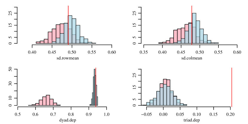
Figure 4: Posterior predictive distributions of goodness of fit statistics for the ordinary regression model (pink) and the SRRM (blue).

1.3 Transitivity and stochastic equivalence via multiplicative effects

It is often observed that the similarity of two nodes $i$ and $j$ in terms of their individual characteristics ${\mathbf{x}}_{i}$ and ${\mathbf{x}}_{j}$ is associated with the value of the relationship $y_{i,j}$ between them. For example, suppose for each node $i$ that $x_{i}$ is the indicator that person $i$ is a member of a particular group or organization. Then $x_{i}x_{j}$ is the indicator that $i$ and $j$ are co-members of this organization, and this fact may have some effect on their relationship $y_{i,j}$. A positive effect of $x_{i}x_{j}$ on $y_{i,j}$ is referred to as homophily, and a negative effect as anti-homophily. Measuring homophily on an observed characteristic can be done within the context of the SRRM by creating a dyadic covariate $x_{d,i,j}$ from a nodal covariate $x_{i}$ through multiplication ($x_{d,i,j}=x_{i}x_{j}$) or some other operation. Homophily on nodal characteristics can lead to certain types of patterns often seen in network and dyadic data, sometimes referred to as transitivity, balance and clustering (Hoff, 2005, 2009). For example, in a binary network where people prefer to form ties to others who are similar to them, there tend to be a lot of “transitive triples,” that is, triples of indices $i,j,k$ having a link between each pair. One explanation of this is that links from $i$ to $j$ and from $i$ to $k$ occur because $i$ is similar to both $j$ and to $k$. If this is the case, then $j$ and $k$ must also be somewhat similar, and so there is a high probability of a link between $j$ and $k$, which would form a triangle of ties among nodes $i$, $j$ and $k$. Multiple linked triangles result in visual “clusters” in graphs of social networks.

More generally, in the case of multiple sender and receiver covariates, we are interested in how a person with characteristics ${\mathbf{x}}_{r,i}$ relates to a person with characteristics ${\mathbf{x}}_{c,j}$. This can be evaluated in the SRRM by including a set of regression terms equivalent to ${\mathbf{x}}_{r,i}^{T}{\mathbf{B}}{\mathbf{x}}_{c,i}$. Although this term is multiplicative in the covariates, it is linear in the parameters, as

$${\mathbf{x}}_{r,i}^{T}{\mathbf{B}}{\mathbf{x}}_{c,i}=\sum_{k}\sum_{l}b_{k,l}x_{r,i,k}x_{c,j,l}$$

and so the matrix of parameters may be estimated within the context of a linear regression model simply by including all products of the elements of ${\mathbf{x}}_{r,i}$ and ${\mathbf{x}}_{c,j}$ as dyadic covariates. In practice, if ${\mathbf{x}}_{r,i}$ and ${\mathbf{x}}_{c,j}$ are of the same length (for example, if they are the same), then it is common to take ${\mathbf{B}}$ to be a diagonal matrix, in which case

$${\mathbf{x}}_{r,i}^{T}{\mathbf{B}}{\mathbf{x}}_{c,i}=b_{1}x_{r,i,1}x_{c,j,1}+\cdots+b_{p}x_{r,i,p}x_{c,j,p}.$$

Such terms in the regression model can often account for network patterns such as transitivity and clustering, as described above. They can also account for another type of network pattern, known as stochastic equivalence, where it is observed that a group of nodes all relate to the other nodes (and each other) in a similar way. If such groups are related to the observed nodal covariates, then often the stochastic equivalence in the data may be estimated and represented by these multiplicative regression terms.

This can be seen to a limited degree in the trade data: Note that the number of shared IGOs and the polity interaction can both be viewed as dyadic covariates obtained by multiplication of nodal covariates. We can fit an SRRM without these effects as follows:

fit_srrm0<-ame(Y,Xd[,,1:2],Xn,Xn)

Figure 5: Comparison of two SRRMs in terms of the triadic dependence statistic: with nodal interaction effects (blue) and without (green).

A comparison of the resulting posterior predictive distribution of the transitivity statistic to that under the full SRRM (which included the multiplicative effects) is given in Figure 5. The figure shows that, while both models do not fully represent the triadic dependence in the data, the model that includes the nodal interactions does slightly better. This raises the possibility that there may exist other nodal attributes, not given in the dataset, whose multiplicative interaction might help further describe the triadic dependence observed in the data. In such cases, it can be useful to include latent nodal characteristics into the regression model, resulting in the following:

$$y_{i,j}=\beta_{d}^{T}{\mathbf{x}}_{d,i,j}+\beta_{r}^{T}{\mathbf{x}}_{r,i}+\beta_{c}^{T}{\mathbf{x}}_{c,j}+a_{i}+b_{j}+{\mathbf{u}}_{i}^{T}{\mathbf{v}}_{j}+\epsilon_{i,j}.$$ (4)

Here, ${\mathbf{u}}_{i}$ is a vector of latent, unobserved factors or characteristics that describe node $i$’s behavior as a sender, and similarly ${\mathbf{v}}_{j}$ describes node $j$’s behavior as a receiver. In this model, the mean of $y_{i,j}$ depends on how “similar” ${\mathbf{u}}_{i}$ and ${\mathbf{v}}_{j}$ are (i.e., the extent to which the vectors point in the same direction) as well as the magnitudes of the vectors. Note also that basic results from matrix algebra indicate that any type of network pattern that could be described by a regression term of the form ${\mathbf{x}}_{r,i}^{T}{\mathbf{B}}{\mathbf{x}}_{c,j}$ can also be described by the multiplicative effects term ${\mathbf{u}}_{i}^{T}{\mathbf{v}}_{j}$.

We call a model of the form (4) an additive and multiplicative effects model, or AME model for network and dyadic data. An AME model essentially combines two models for matrix-valued data: an additive main effects, multiplicative interaction (AMMI) model (Gollob, 1968; Bradu and Gabriel, 1974) - a class of models developed in the psychometric and agronomy literature; and the SRM covariance model that recognizes the dyadic aspect of the data. An AME model, like other latent factor models, requires the specification of the dimension of the latent factors. In the amen package, this can be set with the option R in the ame command. The letter R here stands for “rank”: If ${\mathbf{U}}$ and ${\mathbf{V}}$ are $n\times R$ matrices of the latent factors, then ${\mathbf{U}}{\mathbf{V}}^{T}$ has rank R. For example, a rank-2 AME model may be fit as follows:

fit_ame2<-ame(Y,Xd,Xn,Xn,R=2)

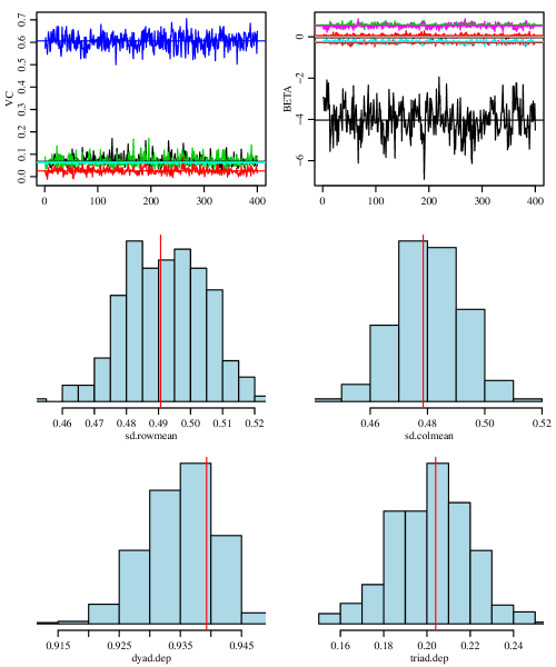
Figure 6: Diagnostic plots for the rank-2 AME model.

The diagnostic plots for this model are given in Figure 6. Note that unlike all previous models considered, this model provides an adequate fit in terms of the triadic dependence statistic. The regression parameter estimates and their standard errors lead to more or less similar conclusions as those from the SRRM, except that the number of shared IGOs no longer has a large effect after controlling for the triadic dependence with the latent factors.

summary(fit_ame2)

Regression coefficients:
                  pmean   psd z-stat p-val
intercept        -4.022 0.764 -5.263 0.000
pop.row          -0.277 0.069 -3.987 0.000
gdp.row           0.568 0.092  6.187 0.000
polity.row        0.000 0.010 -0.022 0.982
pop.col          -0.235 0.071 -3.290 0.001
gdp.col           0.525 0.099  5.315 0.000
polity.col        0.009 0.010  0.826 0.409
conflicts.dyad    0.018 0.036  0.513 0.608
distance.dyad    -0.039 0.004 -9.890 0.000
shared_igos.dyad  0.059 0.070  0.841 0.400
polity_int.dyad  -0.001 0.000 -2.273 0.023

Variance parameters:
    pmean   psd
va  0.072 0.022
cab 0.028 0.016
vb  0.070 0.021
rho 0.605 0.036
ve  0.063 0.004

In some cases it is of interest to examine the estimated latent factors and compare them across nodes. Some ways to do this include clustering the latent factors or simply plotting them. The function circplot in the amen package provides a circle plot that can describe the estimated latent factors of a rank-2 model. A circle plot for the trade data is shown graphically in Figure 7.

Figure 7: Circle plot of estimated latent factors. Directions of $\hat{{\mathbf{u}}}_{i}$’s and $\hat{{\mathbf{v}}}_{i}$’s are given in red and blue, respectively, with the plotting size being a function of the magnitudes of the vectors. Dashed lines between countries indicate greater than expected trade based on the regression terms and additive effects.

Such a figure can help identify groups of nodes that are similar to each other in terms of exporting and importing behavior, after controlling for regression and additive row and column effects. For example, the plot identifies the high trade volume between countries on the Pacific rim.

2 AME models for ordinal data

Often we wish to analyze a dyadic outcome variable that is not well-represented by a normal model. In some cases, such as with the trade data, the variable of interest can be transformed so that the Gaussian AME model is reasonable. In other cases, such as with binary, ordinal, discrete or sparse relations, no such transformation is available. Examples of such data include measures of friendship that are binary (not friends/friends) or ordinal (dislike/neutral/like), discrete counts of conflictual events between countries, or the amount of time two people spend on the phone with each other (which might be zero for most pairs in a population).

In this section we describe extensions of the Gaussian AME model to accommodate ordinal dyadic data, where in what follows, ordinal means any outcome for which the possible values can be put in some meaningful order. This includes discrete outcomes (such as binary indicators or counts), ordered qualitative outcomes (such as low/medium/high, i.e.  the “traditional” definition of ordinal), and even continuous outcomes. The extensions are based on latent variable representations of probit and ordinal probit regression models.

2.1 Example: Analysis of a binary outcome

The simplest type of ordinal dyadic variable is a binary indicator of some type of relationship between $i$ and $j$, so that $y_{i,j}=$ 0 or 1 depending on whether the relationship is absent or present, respectively. Such dyadic data, particularly data indicating social interactions or friendships, are often collectively called a social network. For example, the amen dataset lazegalaw includes a social network of friendship ties between 71 members of a law firm, along with data on two other dyadic variables and several nodal variables. The friendship data are displayed as a graph in Figure 8, where the nodes are colored according to each lawyer’s office location.

data(lazegalaw)

Y<-lazegalaw$Y[,,2]
Xd<-lazegalaw$Y[,,-2]
Xn<-lazegalaw$X

dimnames(Xd)[[3]]

[1] "advice" "cowork"

dimnames(Xn)[[2]]

[1] "status"    "female"    "office"    "seniority" "age"       "practice"
[7] "school"

netplot(lazegalaw$Y[,,2],ncol=Xn[,3])

Figure 8: Graph of the friendship network between 71 lawyers. Node colors represent at which of the three offices each lawyer works.

We first consider fitting a probit SRM model to these binary data, without including any explanatory covariates. This model can be written as

$$z_{i,j} =\mu+a_{i}+b_{j}+\epsilon_{i,j}$$ (5)

$$y_{i,j} =1(z_{i,j}>0),$$ (6)

where the distributions of the random effects $a_{i}$, $b_{j}$, and $\epsilon_{i,j}$ follow the Gaussian SRM covariance model as described previously. This model expresses the observed binary variable $y_{i,j}$ as the indicator that some continuous latent variable $z_{i,j}$ exceeds zero. Assuming the SRM for the sociomatrix ${\mathbf{Z}}=\{z_{i,j}\}$ of latent variables yields a model for the observed binary data that allows for within-row, within-column and within-dyad dependence. This model can be fit with the ame command by specifying that the variable type is binary:

fit_SRM<-ame(Y,model="bin")

It is instructive to compare the fit of this model to that provided by a reduced model that lacks the SRM terms:

fit_SRG<-ame(Y,model="bin",rvar=FALSE,cvar=FALSE,dcor=FALSE)

This is a probit model that contains only an intercept, and so is equivalent to the simple random graph model (SRG). The fits of these two models in terms of the four goodness of fit statistics computed by gofstats are compared in Figure 9. As might be expected, the SRG fails in terms of all four statistics. In contrast, the SRM model provides a good fit in terms of the three statistics that represent second-order dependence. Both models fail in terms of representing third-order dependence.

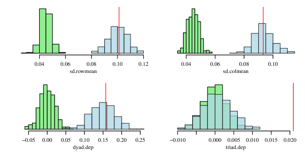
Figure 9: Comparison of the SRM (blue) and the SRG (green) for the Lazega law friendship network.

A common empirical description of row and column heterogeneity in network data are the row and column sums, typically referred to as the outdegrees and indegrees. Based on the form of the model in (5), we might expect that the outdegrees and indegrees would be positively associated with the estimates of the $a_{i}$’s and $b_{j}$’s respectively. For example, the larger $a_{i}$ is, the larger the entries of $z_{i,j}$ for each $j$, thereby making more of the $y_{i,j}$’s equal to one rather than zero. This relationship between the degrees and the parameter estimates is illustrated in Figure 10. The figure does indeed show a strong positive association between these quantities, but note that the relationship is not strictly monotonic. The reason for this can be explained by the fact that it is both the $a_{i}$ parameters and the $b_{j}$ parameters that are used to describe nodal heterogeneity. For example, suppose two nodes have the same outdegree, but the first links to several nodes that have low indegrees, whereas a second node links to the same number of nodes but ones having high indegrees. The first node will have an $a_{i}$ estimate that is higher than that of the second, because the $b_{j}$’s of the nodes that the first links to will be lower than those of the nodes that the second links to.

Figure 10: Estimated row and column effects versus outdegrees and indegrees.

We next consider a probit SRRM that includes the SRM terms and linear regression effects for some nodal and dyadic covariates. This model is formulated as in the SRM probit model, except that $z_{i,j}$ follows an SRRM rather than an SRM.

Xno<-Xn[,c(1,2,4,5,6)]
fit_SRRM<-ame(Y, Xd=Xd, Xr=Xno, Xc=Xno, model="bin")

summary(fit_SRRM)

Regression coefficients:
               pmean   psd z-stat p-val
intercept      0.882 0.659  1.338 0.181
status.row    -0.174 0.175 -0.992 0.321
female.row     0.007 0.143  0.051 0.959
seniority.row -0.008 0.012 -0.675 0.500
age.row       -0.016 0.009 -1.722 0.085
practice.row  -0.227 0.109 -2.089 0.037
status.col    -0.168 0.145 -1.154 0.248
female.col    -0.027 0.123 -0.219 0.827
seniority.col  0.012 0.011  1.056 0.291
age.col       -0.008 0.008 -1.064 0.287
practice.col  -0.286 0.110 -2.602 0.009
advice.dyad   -0.080 0.075 -1.069 0.285
cowork.dyad    1.281 0.063 20.313 0.000

Variance parameters:
    pmean   psd
va  0.170 0.037
cab 0.012 0.025
vb  0.134 0.032
rho 0.110 0.048
ve  1.000 0.000

There is not much evidence for effects of the nodal characteristics, at least in terms of effects that appear linearly in the SRRM. Additionally, goodness-of-fit plots indicate lack of fit in terms of triadic dependence, as with the SRM model. Thus, we consider instead a model with the “non-significant” regressors removed, and include a rank-3 multiplicative effect.

fit_AME<-ame(Y, Xd=Xd[,,2], R=3, model="bin")

Figure 11: Checks of the fit of the rank-3 AME model to the Lazega law friendship network.

The goodness-of-fit plots in Figure 11 indicate no strong discrepancy between this model and the data in terms of these statistics. Inference then proceeds by examining the estimates of regression effects, random effects and covariance parameters. Interpretation of the multiplicative effects can proceed by plotting them, looking for clusters, and identification of nodes with large effects. Additionally, it can be useful to look for associations between the multiplicative effects and any nodal characteristics available. For example, we can compute correlations between the multiplicative effects $({\mathbf{u}}_{i},{\mathbf{v}}_{i})$ and any numerical or ordinal nodal characteristics ${\mathbf{x}}_{i}$. Associations between multiplicative effects and categorical variables can be examined via plots.

U<-fit_AME$U
V<-fit_AME$V

round(cor(U, Xno),2)

     status female seniority   age practice
[1,]  -0.12  -0.02     -0.20 -0.25     0.00
[2,]  -0.34  -0.04      0.24  0.26     0.62
[3,]  -0.03   0.28     -0.01  0.12     0.20

round(cor(V, Xno),2)

     status female seniority  age practice
[1,]  -0.81  -0.32      0.71 0.62     0.24
[2,]  -0.04   0.15     -0.06 0.00     0.55
[3,]  -0.06   0.14      0.26 0.31     0.20

These correlations, and the plots in Figure 12, indicate that these nodal characteristics do play a role in network formation, although in a multiplicative rather than additive manner. If desired, one could use these results to construct multiplicative functions of these nodal attributes for inclusion into a SRRM, or possibly an AME model of lower rank.

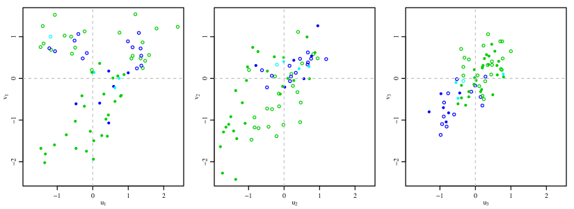
Figure 12: Estimated latent factors plotted in terms of the nodal characteristics status (partner=unfilled circle, associate=filled circle) and office (Boston=green, Hartford=blue, Providence=light blue).

2.2 Example: Analysis of an ordinal outcome

The probit AME model for binary data extends in a natural way to accommodate ordinal data with more than two levels. As with binary data, we model the sociomatrix ${\mathbf{Y}}=\{y_{i,j}\}$ as being a function of a latent sociomatrix ${\mathbf{Z}}$ that follows a Gaussian AME model. Specifically, our model is

$$z_{i,j} =\beta_{d}^{T}{\mathbf{x}}_{d,i,j}+\beta_{r}^{T}{\mathbf{x}}_{r,i}+\beta_{c}^{T}{\mathbf{x}}_{c,j}+a_{i}+b_{j}+\epsilon_{i,j},$$ (7)

$$y_{i,j} =g(z_{i,j}),$$

where $g$ is some unknown non-decreasing function. The amen package takes a semiparametric approach to this model, providing estimation and inference for the parameters in the model (7) for ${\mathbf{Z}}$, but treating the function $g$ as a nuisance parameter. This is done using a variant of the extended rank likelihood for ordinal data, described in Hoff (2007) and Hoff (2008b). While this approach is somewhat limiting (as estimation of $g$ is not specifically provided), it simplifies some aspects of model specification and parameter estimation. In particular, the semiparametric approach allows for modeling of more general types of ordinal variables $y_{i,j}$, such as those that are continuous, or those for which the number of levels is not pre-specified. However, we caution that the computation time required by the MCMC algorithm used by amen is increasing in the number of levels of $y_{i,j}$.

We illustrate this model fitting procedure with an analysis of dominance relations between 28 female bighorn sheep, available via the sheep dataset included with amen. The dyadic variable $y_{i,j}$ records the number of times sheep $i$ was observed dominating sheep $j$.

data(sheep)

Y<-sheep$dom

gofstats(Y)

 sd.rowmean  sd.colmean    dyad.dep   triad.dep
 0.70037477  0.67209344 -0.19797403 -0.05826448

Note that the dyadic dependence and triadic dependence statistics are negative. This makes sense in light of the nature of the variable: Heterogeneity among the sheep in terms of strength or assertiveness would lead to powerful sheep dominating but not being dominated by others, thus leading to negative reciprocity. Additionally, under this scenario, if sheep $i$ dominated $j$, and $j$ dominated $k$, then it is unlikely that $k$ would be able to dominate $i$. Such a scenario would lead to negative triadic dependence.

Data on the ages of the sheep are also available. Plots of row and column means versus age are given in Figure 13, and indicate some evidence of an age effect. Particularly, the number of times that a sheep is dominated is decreasing on average with age. We examine this effect more fully with an ordinal probit regression, fitting a second-degree polynomial in the ages of the sheep:

Figure 13: Plots of the sheep dominance data. From left to right, a histogram of the number of dominance encounters, age versus row mean, and age versus column mean.

x<-sheep$age - mean(sheep$age)

Xd<-outer(x,x)

Xn<-cbind(x,x^2) ; colnames(Xn)<-c("age","age2")

fit<-ame(Y, Xd, Xn, Xn, model="ord")

summary(fit)

Regression coefficients:
          pmean   psd z-stat p-val
age.row   0.158 0.051  3.101 0.002
age2.row -0.086 0.019 -4.454 0.000
age.col  -0.241 0.039 -6.136 0.000
age2.col -0.008 0.015 -0.561 0.575
.dyad     0.043 0.008  5.370 0.000

Variance parameters:
     pmean   psd
va   0.433 0.153
cab  0.039 0.073
vb   0.215 0.084
rho -0.399 0.091
ve   1.000 0.000

The results indicate evidence for a positive effect of age on dominance - older sheep are more likely to dominate and less likely to be dominated. The dyadic effect reflects some residual effect of homophily by age: A young sheep’s dominance encounters are typically with other young sheep, and older sheep are more likely to be dominated by another older sheep than a younger sheep.

Also note that the summary of the model fit does not include an intercept. This is because the intercept is not identifiable using the rank likelihood approach used to obtain the parameter estimates. Specifically, an intercept term can be thought of as part of the transformation function $g$, which is being treated as a nuisance parameter.

3 Censored and fixed rank nomination data

Data on human social networks are often obtained by asking members of a study population to name a fixed number of people with whom they are friends, and possibly to rank these friends in terms of their affinities to them. Such a survey method is called a fixed rank nomination (FRN) scheme, and is commonly used in studies of institutions such as schools or businesses. For example, the National Longitudinal Study of Adolescent Health (AddHealth, Harris et al. (2009)) asked middle and high-school students to nominate and rank up to five members of the same sex as friends, and five members of the opposite sex as friends.

Data obtained from FRN schemes are similar to ordinal data, in that the ranks of a person’s friends may be viewed as an ordinal response. However, FRN data are also censored in a complicated way. Consider a study where people were asked to name and rank up to and including their top five friends. If person $i$ nominates five people but doesn’t nominate person $j$, then $y_{i,j}$ is censored: The data cannot tell us whether $j$ is $i$’s sixth best friend, or whether $j$ is not liked by $i$ at all. On the other hand, if person $i$ nominates four people as friends but could have nominated five, then person $i$’s data are not censored - the absence of a nomination by $i$ of $j$ indicates that $i$ does not consider $j$ a friend.

A likelihood-based approach to modeling FRN data was developed in Hoff et al. (2013). Similar to the approach for ordinal dyadic data described above, this methodology treats the observed ranked outcomes ${\mathbf{Y}}$ as a function of an underlying continuous sociomatrix ${\mathbf{Z}}$ of affinities that is generated from an AME model. Letting $m$ be the maximum number of nominations allowed, and coding $y_{i,j}\in\{m,m-1,\ldots,1,0\}$ so that $y_{i,j}=m$ indicates that $j$ is $i$’s most liked friend, the FRN likelihood is derived from the following constraints that the observed ranks ${\mathbf{Y}}$ tell us about the underlying dyadic variables ${\mathbf{Z}}$:

$$y_{i,j}>0 \Rightarrow z_{i,j}>0$$ (8)

$$y_{i,j}>y_{i,k} \Rightarrow z_{i,j}>z_{i,k}$$ (9)

$$y_{i,j}=0\ \mbox{and}\ d_{i}<m \Rightarrow z_{i,j}\leq 0.$$ (10)

Constraint (8) indicates that if $i$ ranks $j$, then $i$ has a positive relation with $j$ ($z_{i,j}>0$), and constraint (9) indicates that a higher rank corresponds to a more positive relation. Letting $d_{i}\in\{0,\ldots,m\}$ be the number of people that $i$ ranks, constraint (10) indicates that if $i$ could have made additional friendship nominations but chose not to nominate $j$, they then must not consider $j$ a friend. On the other hand, if $y_{i,j}=0$ but $d_{i}=m$ then person $i$’s unranked relationships are censored, and so $z_{i,j}$ could be positive even though $y_{i,j}=0$. In this case, all that is known about $z_{i,j}$ is that it is less than $z_{i,k}$ for any person $k$ that is ranked by $i$.

3.1 Example: Analysis of fixed rank nomination data

The amen package implements a Bayesian model fitting algorithm based on the FRN likelihood. We illustrate its use with an analysis of data from the classic study on relationships between monks described in Sampson (1969), in which each monk was asked to rank up to three other monks in terms of a variety of relations.

Y<-sampsonmonks[,,3]

apply(Y>0,1,sum,na.rm=T)

  ROMUL BONAVEN AMBROSE   BERTH   PETER   LOUIS  VICTOR    WINF    JOHN
      3       3       4       3       3       3       3       3       3
   GREG    HUGH    BONI    MARK  ALBERT   AMAND   BASIL   ELIAS    SIMP
      4       3       3       3       3       3       3       3       3

Notice that two of the monks didn’t follow the survey instructions, and nominated more than three other monks. We treat the maximum number of nominations for these two monks as four. This can be done using the ame fitting function, and specifying the FRN likelihood and the number of maximum nominations as follows:

odmax<-rep(3,nrow(Y))
odmax[ apply(Y>0,1,sum,na.rm=T)>3 ]<-4

fit<-ame(Y,R=2,model="frn",odmax=odmax)

summary(fit)

Regression coefficients:
          pmean   psd z-stat p-val
intercept  0.64 0.725  0.883 0.377

Variance parameters:
    pmean   psd
va  0.557 0.768
cab 0.006 0.152
vb  0.249 0.185
rho 0.761 0.164
ve  1.000 0.000

Goodness of fit plots for these data appear in Figure 14. Notice that the fit in terms of row heterogeneity is very good. This is not too surprising: The simulated sociomatrices used to produce this plot are generated to satisfy the constraint imposed the outdegree constraint imposed by odmax, which greatly limits the possible amount of outdegree heterogeneity.

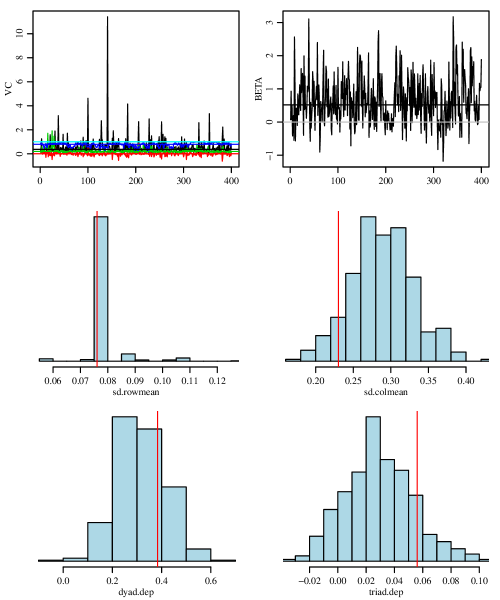
Figure 14: Model fitting plots for Sampson’s monk data.

3.2 Other approaches to censored or ranked data

Some dyadic survey designs ask participants to nominate up to a certain number of friends, but not to rank them. Such dyadic data are binary, but censored in the same way as are data from an FRN survey: Observing that $y_{i,j}=0$ indicates that $i$ is not friends with $j$ only if person $i$ has made less than the maximum number of nominations. A likelihood-based approach to analyzing such censored binary data is described in Hoff et al. (2013) and is also implemented in the amen package using the model="cbin" option in the ame command.

In other situations the dyadic outcomes in each row are ordinal, but on completely different scales. In such cases, we may wish to treat the heterogeneity of ties across rows in a semiparametric way, and only estimate the parameters in the AME model based on the ranks of the outcomes within each row. This can be done by using a likelihood for which the ordinal dyadic data ${\mathbf{Y}}$ only imposes constraint (9) on the unobserved underlying variables ${\mathbf{Z}}$. This “relative rank likelihood” is described more fully in Hoff et al. (2013), and can be implemented in amen using the model="rrl" option in the ame command.

4 Sampled or missing dyadic data

Some dyadic datasets are only partially observed, in that the value of $y_{i,j}$ is not observed for all pairs $i,j$. This can happen unintentionally or by design. For example, to avoid the cost of measuring $y_{i,j}$ for all $n(n-1)$ ordered pairs of nodes, some researchers use multi-stage link-tracing designs, in which nodes are selected into the study in one stage of the design based on their links to nodes included in previous stages.

Partially observed dyadic data on a given nodeset can be represented by a sociomatrix in which the ordered pairs for which data are not observed are distinguished from pairs for which data are observed. In R, this is done by filling each entry of the sociomatrix corresponding to a missing value with an “NA”. Doing so distinguishes pairs $i,j$ for which we do not know the dyadic value $(y_{i,j}={\tt NA})$ from those, for example, for which we know there is no link $(y_{i,j}=0)$.

When some (non-diagonal) entries of the sociomatrix ${\mathbf{Y}}$ are missing, the MCMC approximation algorithm used by amen proceeds by iteratively simulating model parameters along with values for the missing values in a way that approximates their joint posterior distribution. Roughly speaking, at each iteration of the MCMC algorithm, values for the missing values are simulated from their probability distribution conditional on the observed data and the current values of the model parameters. Such a procedure is appropriate if the missing values are missing at random, or more specifically, if the study design is ignorable. A study design is ignorable if the probability of a missing data value for a pair is independent of the model parameters and missing values, conditional on the observed data values. Many types of link tracing designs, such as egocentric and snowball sampling, are ignorable (Thompson and Frank, 2000).

4.1 Example: Analysis of an egocentric sample

One popular and relatively inexpensive design for gathering dyadic data is with an egocentric sample, in which nodes (or “egos”) are randomly sampled from a population and then asked about their ties and the ties between their friends. For example, one type of egocentric study design might ask participants “with whom are you friends” and “which of your friends are friends with each other.” Data from such a design can be sufficient to estimate parameters in an AME model.

We illustrate this with an example analysis of the effect of sex (male/female) on friendships among a small group of Dutch college students, available in amen from the dutchcollege dataset.

data(dutchcollege)

Y<-1*( dutchcollege$Y[,,7] > 1 ) # indicator of positive relationship at the last timepoint

Xn<-dutchcollege$X[,1]           # nodal indicator of male sex
Xd<-1*(outer(Xn,Xn,"=="))        # dyadic indicator of same sex

We will fit a simple SRRM to these data, and then compare the resulting parameter estimates to those based on data obtained from the egocentric design described above. In our design, we first randomly sample several nodes (egos), record their relationships to the other nodes, and then record the relationships between alters having a common ego. R-code that generates such a design is as follows:

n<-nrow(Y)
Ys<-matrix(NA,n,n)      # sociomatrix for sampled data

egos<-sort(sample(n,5)) # ego sample
Ys[egos,]<-Y[egos,]     # relations of egos are observed

for(i in egos)
{
  ai<-which(Ys[i,]==1)  # alters of i  
  Ys[ai,ai]<-Y[ai,ai]   # relations between alters of i are observed
}

mean(is.na(Ys))

[1] 0.7314453

This particular instance of the design results in a sociomatrix where about 73 percent of the entries are missing (note that the diagonal is already “missing” by definition). Under this design, data between alters and non-alters of an ego are missing, as are data between alters that do not share an ego.

egos

[1]  6 10 12 17 26

Ys[1:10,1:10]

      [,1] [,2] [,3] [,4] [,5] [,6] [,7] [,8] [,9] [,10]
 [1,]   NA   NA   NA   NA   NA   NA   NA   NA   NA    NA
 [2,]   NA   NA    0   NA   NA   NA    0    0   NA     1
 [3,]   NA    0   NA   NA   NA   NA    1    0   NA    NA
 [4,]   NA   NA   NA   NA   NA   NA   NA   NA   NA    NA
 [5,]   NA   NA   NA   NA   NA   NA   NA   NA   NA    NA
 [6,]    0    0    0    0    0   NA    0    0    0     0
 [7,]   NA    0    1   NA   NA   NA   NA    1   NA    NA
 [8,]   NA    0    0   NA   NA   NA    0   NA   NA     1
 [9,]   NA   NA   NA   NA   NA   NA   NA   NA   NA    NA
[10,]    0    1    1    0    0    0    1    1    0    NA

We now fit an SRRM model to the complete data and the subsampled data, and compare parameter estimates.

fit_pop<-ame(Y,Xd,Xn,Xn,model="bin")   # fit based on full data (population) 

fit_ess<-ame(Ys,Xd,Xn,Xn,model="bin")  # fit based on egocentric subsample

apply(fit_pop$BETA,2,mean)

 intercept       .row       .col      .dyad
-1.8662999  0.3172635  0.3824924  0.7365514

apply(fit_ess$BETA,2,mean)

 intercept       .row       .col      .dyad
-2.1561520  0.3172207  1.1966069  0.9929780

The estimates are similar, even though the second fit is from a dataset with 73 missing values.

The output of the ame fitting procedure also includes a posterior predictive mean for all entries of the sociomatrix ${\mathbf{Y}}$, including those entries for which the data are missing. This sociomatrix of predicted values can be used for prediction or imputation of dyadic data from incomplete datasets. In our example on modeling friendship relations from the dutchcollege dataset, we can use this sociomatrix of predicted values to evaluate how well the parameter estimates obtained from the sampled dataset compare to those obtained from the full dataset, in terms of prediction:

miss<-which(is.na(Ys))

mean( ( fit_pop$YPM[miss] - Y[miss] )^2, na.rm=TRUE )

[1] 0.09428416

mean( ( fit_ess$YPM[miss] - Y[miss] )^2, na.rm=TRUE )

[1] 0.1350285

The first and second numbers reflect “within-sample” and “out-of-sample” goodness of fit, respectively. The small discrepancy between these numbers indicates that reasonable parameter estimates for this model (in terms of out-of-sample predictive squared error) can be obtained from this egocentric sample.

Finally, we consider the variability of the parameter estimates across egocentric samples with a small simulation study: For each of 100 egocentric samples randomly generated as previously described, we obtain parameter estimates for the probit SRRM,

$$z_{i,j} =\beta_{0}+\beta_{r}x_{i}+\beta_{c}x_{j}+\beta_{d}x_{i,j}+\epsilon_{i,j}$$

$$y_{i,j} =1(z_{i,j}>0),$$

where $x_{i}$ is a binary indicator that node $i$ is male, and $x_{i,j}$ is the indicator that $i$ and $j$ are of the same sex. The variability of the parameter estimates across egocentric samples is illustrated with histograms in Figure 15. An illustrative exercise would be to see how increasing or decreasing the amount of missing data in the samples (by increasing or decreasing the number of egos sampled) would affect the concentration of the egocentric estimates around the population estimates.

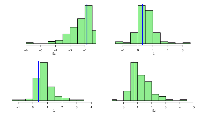
Figure 15: Variability of probit SRRM regression estimates across egocentric samples. Vertical blue lines indicate the estimates obtained from the full (population) dataset.

5 Repeated measures data

Some types of dynamic dyadic datasets include repeated measurements of dyadic and nodal variables at discrete points in time. The amen package provides a rudimentary method of analyzing such data, based on the following simple extension of the AME model to accommodate replicated dyadic measurements: For (latent) sociomatrices ${\mathbf{Z}}_{1},\ldots,{\mathbf{Z}}_{T}$, the model expresses $z_{i,j,t}$, the $(i,j)$th element of the $t$th sociomatrix, as

$$z_{i,j,t}=\beta_{d}^{T}{\mathbf{x}}_{d,i,j,t}+\beta_{r}^{T}{\mathbf{x}}_{r,i,j,t}+\beta_{c}^{T}{\mathbf{x}}_{c,i,j,t}+a_{i}+b_{j}+{\mathbf{u}}_{i}^{T}{\mathbf{v}}_{j}+\epsilon_{i,j,t}.$$ (11)

Across nodes, dyads and time points, this model extension further assumes the same covariance model for the random effects $\{(a_{i},b_{i})\}$ as before, allows for dyadic correlation between $\epsilon_{i,j,t}$ and $\epsilon_{j,i,t}$ as before, but assumes that $\epsilon_{i,j,t}$’s from different dyads or different time points are independent. In other words, the data under this model are treated as independent observations from a common AME distribution.

At first glance it may seem that such a model is inappropriate for dynamic dyadic data, as it doesn’t seem to allow for the possibility of dependence over time. However, certain types of dependence can be incorporated into this model via the time-dependent regression terms. For example, autoregressive dependence can be modeled by including lagged values of the sociomatrix as predictors. Additionally, time-varying regression parameters can be included in the model by constructing interactions.

5.1 Example: Analysis of a longitudinal binary outcome

We illustrate these possibilities with an analysis of data from the longitudinal study of friendship relations among a small group of Dutch college students, available in amen via the dutchcollege dataset. Our response $y_{i,j,t}$ is the indicator that person $i$ reports being friendly (or having friendship) with person $j$ at time point $t$. The graphs of this variable for each of the seven different time points in the dataset are given in Figure 16.

Figure 16: Friendliness network of the Dutch college students, across seven time points.

The figure reflects the fact that the students were mostly unknown to each other before the study period, and so not surprisingly, the densities of the graphs increase over time.

The data also include (static) information on the sex and smoking status of the students, as well as which one of three programs each student was a member. We will examine the effects of these nodal attributes on friendship in using a probit SRRM, where $y_{i,j,t}$ is modeled as the indicator that the latent affinity $z_{i,j,t}$ exceeds zero, where $z_{i,j,t}$ follows model (11). Our analysis will include the binary indicators of male sex and smoking status as row and column regressors, products of these variables as dyadic regressors, and a dyadic binary indicator of whether or not members of a dyad belong to the same program. Finally, we will also include lagged values $y_{i,j,t-1}$ and $y_{j,i,t-1}$ as dyadic predictors of $z_{i,j,t}$ to reflect the possibility of temporal dependence among values within a dyad. To summarize, our model for the $z_{i,j,t}$’s is as follows:

$$z_{i,j,t}= \beta_{0}+$$

$$\beta_{r,1}\text{male}_{i}+\beta_{r,2}\text{smoke}_{i}+$$

$$\beta_{c,1}\text{male}_{j}+\beta_{c,2}\text{smoke}_{j}+$$

$$\beta_{d_{1}}y_{i,j,t-1}+\beta_{d_{2}}y_{j,i,t-1}+$$

$$\beta_{d_{3}}\text{male}_{i}\text{male}_{j}+\beta_{d_{4}}\text{smoke}_{i}\text{smoke}_{j}+\beta_{d_{5}}\text{sameprogram}_{i,j}+$$

$$a_{i}+b_{j}+\epsilon_{i,j,t}$$

The ame_rep function in the amen package provides parameter estimation and inference for this model using a similar syntax as the ame function, except now the nodal attributes Xrow and Xcol are three-dimensional arrays, with dimensions corresponding to nodes, variables and time points, respectively. Similarly, the dyadic regressor array Xdyad is now four-dimensional, with dimensions corresponding to nodes, nodes, variables and time points. These arrays for this data analysis can be set up as follows:

# outcome
Y<-1*( dutchcollege$Y >= 2 )[,,2:7]
n<-dim(Y)[1] ; t<-dim(Y)[3]

# nodal covariates
Xnode<-dutchcollege$X[,1:2]                                       # sex and smoking status
Xnode<-array(Xnode,dim=c(n,ncol(Xnode),t))
dimnames(Xnode)[[2]]<-c("male","smoker")

# dyadic covariates
Xdyad<-array(dim=c(n,n,5,t))
Xdyad[,,1,]<-1*( dutchcollege$Y >= 2 )[,,1:6]                     # lagged value
Xdyad[,,2,]<-array(apply(Xdyad[,,1,],3,t),dim=c(n,n,t))           # lagged reciprocal value 
Xdyad[,,3,]<-tcrossprod(Xnode[,1,1])                              # both male
Xdyad[,,4,]<-tcrossprod(Xnode[,2,1])                              # both smokers 
Xdyad[,,5,]<-outer( dutchcollege$X[,3],dutchcollege$X[,3],"==")   # same program
dimnames(Xdyad)[[3]]<-c("Ylag","tYlag","bothmale","bothsmoke","sameprog")

The model can be fit using the same syntax as the ame command discussed previously, and results can summarized before with the summary function:

fit_ar1<-ame˙rep(Y,Xdyad,Xnode,Xnode,model="bin",plot=FALSE)

summary(fit_ar1)

Regression coefficients:
                pmean   psd z-stat p-val
intercept      -1.612 0.170 -9.457 0.000
male.row       -0.170 0.220 -0.772 0.440
smoker.row     -0.458 0.182 -2.516 0.012
male.col       -0.038 0.162 -0.236 0.813
smoker.col     -0.236 0.145 -1.627 0.104
Ylag.dyad       1.201 0.063 19.146 0.000
tYlag.dyad      0.860 0.062 13.796 0.000
bothmale.dyad   0.740 0.145  5.090 0.000
bothsmoke.dyad  0.661 0.122  5.424 0.000
sameprog.dyad   0.432 0.063  6.880 0.000

Variance parameters:
    pmean   psd
va  0.223 0.073
cab 0.033 0.034
vb  0.119 0.038
rho 0.641 0.038
ve  1.000 0.000

The parameter estimates and standard deviations for $\beta_{d,1}$ and $\beta_{d,2}$ (Ylag.dyad and tYlag.dyad in the output) indicate strong evidence of large temporal correlation. There also appears to be strong homophily effects in terms of sex, smoking status and program. The nodal effect parameters indicate some evidence that smokers are a bit less social than non-smokers.

Finally, we note that the time interval between the first four measurements was three weeks, whereas the interval between the last three measurements was six weeks. As such, we may want to consider whether or not the effects of the regressors might vary depending on the time lag between measurements. Such a possibility can be evaluated simply by adding interaction terms to the regressors. For example, to evaluate whether or not the effect of $y_{i,j,t-1}$ on $z_{i,j,t}$ varies with measurement interval, we can create a new dyadic covariate $y_{i,j,t-1}w_{t}$ where $w_{t}$ is a binary indicator that $t$ is among the last three measurements. Adding such terms for all of our regressors can be done as follows:

Wnode<-Xnode
Wnode[,,1:3]<-0

XWnode<-array( dim=dim(Xnode)+c(0,2,0))
XWnode[,1:2,]<-Xnode ; XWnode[,3:4,]<-Wnode
dimnames(XWnode)[[2]]<-c(dimnames(Xnode)[[2]],paste0(dimnames(Xnode)[[2]],".w"))


Wdyad<-Xdyad
Wdyad[,,,1:3]<-0
XWdyad<-array( dim=dim(Xdyad)+c(0,0,5,0) )
XWdyad[,,1:5,]<-Xdyad ; XWdyad[,,6:10,]<-Wdyad
dimnames(XWdyad)[[3]]<-c(dimnames(Xdyad)[[3]],paste0(dimnames(Xdyad)[[3]],".w"))

fit_ar1_vb<-ame˙rep(Y,XWdyad,XWnode,XWnode,model="bin")

summary(fit_ar1_vb)

Regression coefficients:
                  pmean   psd z-stat p-val
intercept        -1.606 0.167 -9.625 0.000
male.row         -0.313 0.238 -1.311 0.190
smoker.row       -0.374 0.204 -1.833 0.067
male.w.row        0.240 0.141  1.696 0.090
smoker.w.row     -0.156 0.137 -1.134 0.257
male.col         -0.068 0.171 -0.395 0.693
smoker.col       -0.208 0.148 -1.402 0.161
male.w.col        0.036 0.133  0.268 0.788
smoker.w.col     -0.048 0.120 -0.403 0.687
Ylag.dyad         1.400 0.101 13.797 0.000
tYlag.dyad        0.855 0.109  7.839 0.000
bothmale.dyad     1.009 0.209  4.831 0.000
bothsmoke.dyad    0.558 0.165  3.373 0.001
sameprog.dyad     0.334 0.080  4.169 0.000
Ylag.w.dyad      -0.296 0.122 -2.432 0.015
tYlag.w.dyad     -0.008 0.131 -0.059 0.953
bothmale.w.dyad  -0.520 0.277 -1.875 0.061
bothsmoke.w.dyad  0.194 0.225  0.864 0.387
sameprog.w.dyad   0.187 0.097  1.924 0.054

Variance parameters:
    pmean   psd
va  0.224 0.075
cab 0.032 0.036
vb  0.116 0.038
rho 0.650 0.037
ve  1.000 0.000

These results do not indicate much evidence that the regression coefficients should vary by time period, except possibly the effect on the lagged dyadic variable $y_{i,j,t}$. The negative estimate of this coefficient (corresponding to Ylag.w.dyad in the output) makes sense, as it indicates that the effect of the lagged variable is decreased when the interval between times points is longer.

6 Symmetric data

It is sometimes the case that dyadic observations are symmetric or undirected by design, in that there is only one value $y_{i,j}$ for the dyad $\{i,j\}$. Such observations can be represented by a symmetric sociomatrix ${\mathbf{Y}}$, so that $y_{i,j}=y_{j,i}$ for all dyads $\{i,j\}$. In this case, a natural simplification of the AME model (4) is given by

$$y_{i,j} =\beta_{d}^{T}{\mathbf{x}}_{i,j}+\beta_{n}^{T}({\mathbf{x}}_{i}+{\mathbf{x}}_{j})+a_{i}+a_{j}+{\mathbf{u}}_{i}^{T}{\mathbf{\Lambda}}{\mathbf{u}}_{j}+\epsilon_{i,j},$$ (12)

$$a_{1},\ldots,a_{n} \sim\text{i.i.d.}\ N(0,\sigma^{2}_{a})$$

$$\{\epsilon_{i,j}\} \sim\text{i.i.d.}\ N(0,\sigma^{2}_{e}),$$

for $i<j$, with $y_{j,i}=y_{i,j}$ by design. Most of the simplifications leading to this symmetric model are easy to understand, with the possible exception of the change from ${\mathbf{u}}_{i}^{T}{\mathbf{v}}_{j}$ in the asymmetric case to ${\mathbf{u}}_{i}^{T}{\boldsymbol{\Lambda}}{\mathbf{u}}_{j}$ here. In the former case, this representation can be justified by the singular value decomposition theorem, which states that any $n\times n$ rank-$R$ matrix ${\mathbf{M}}$ can be expressed as ${\mathbf{U}}{\mathbf{V}}^{T}$, where ${\mathbf{U}}$ and ${\mathbf{V}}$ are ${n\times R}$ matrices. This means that $m_{i,j}$, the $i,j$th entry of ${\mathbf{M}}$ can be expressed as $m_{i,j}={\mathbf{u}}_{i}^{T}{\mathbf{v}}_{j}$, where ${\mathbf{u}}_{i}$ and ${\mathbf{v}}_{j}$ are the $i$th and $j$th rows of ${\mathbf{U}}$ and ${\mathbf{V}}$, respectively. In other words, the ${\mathbf{u}}_{i}^{T}{\mathbf{v}}_{j}$ in the asymmetric AME model can represent any residual low-rank patterns ${\mathbf{M}}$ in the sociomatrix ${\mathbf{Y}}$ that aren’t explained by the known regressors. Similarly, in the symmetric case the term ${\mathbf{u}}_{i}^{T}{\boldsymbol{\Lambda}}{\mathbf{u}}_{j}$ in (12) can represent any residual low-rank patterns ${\mathbf{M}}$ in the symmetric sociomatrix ${\mathbf{Y}}$. This follows from the eigenvalue decomposition theorem, which states that any symmetric rank-$R$ matrix ${\mathbf{M}}$ can be expressed as ${\mathbf{U}}{\boldsymbol{\Lambda}}{\mathbf{U}}^{T}$, or equivalently, the elements $m_{i,j}$ of ${\mathbf{M}}$ can be expressed as $m_{i,j}={\mathbf{u}}_{i}^{T}{\boldsymbol{\Lambda}}{\mathbf{u}}_{j}$. Furthermore, as with the asymmetric case, such a latent factor model can represent patterns of transitivity and stochastic equivalence in network data (Hoff, 2008a).

6.1 Example: Analysis of a symmetric ordinal outcome

Symmetric versions of the normal, probit and other AME models discussed in the previous sections can be fit by simply specifying the option symmetric=TRUE in the ame command. We illustrate the use of this option with an analysis of Cold War cooperation and conflict data, available via the coldwar dataset. These data include dyadic counts of military cooperation and conflict between countries, geographic distances between countries, and country-level measures of GDP and polity. These variables were recorded every five years from 1950 to 1985. For simplicity, we analyze a time-averaged version of the dataset:

data(coldwar)

# response
Y<-sign( apply(coldwar$cc,c(1,2), mean ) )

# nodal covariates
Xn<-cbind( apply( log(coldwar$gdp),1,mean ) ,       # log gdp
           sign(apply(coldwar$polity ,1,mean ) ) )  # sign of polity      
Xn[,1]<-Xn[,1]-mean(Xn[,1])
dimnames(Xn)[[2]]<-c("lgdp","polity")

# dyadic covariates
Xd<-array(dim=c(nrow(Y),nrow(Y),3))
Xd[,,1]<- tcrossprod(Xn[,1])                        # gdp interaction
Xd[,,2]<- tcrossprod(Xn[,2])                        # polity interaction
Xd[,,3]<-log(coldwar$distance)                      # log distance
dimnames(Xd)[[3]]<-c("igdp","ipol","ldist")

The response $y_{i,j}$ takes values in $\{-1,0,1\}$. As such, we view this as an ordinal outcome, to which we fit an ordinal version of a rank-1 symmetric AME model using the ame command:

fit_cw_R1<-ame(Y,Xd,Xn,R=1,model="ord",symmetric=TRUE,burn=1000,nscan=100000,odens=100)

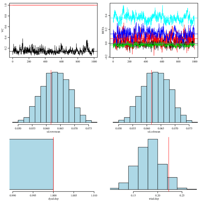
Figure 17: Diagnostic plots for the rank-1 AME model of the coldwar data.

Note that for this symmetric model, the row regressors must be the same as the column regressors, and so it is sufficient to specify these just once. We also note that for technical reasons, the mixing of the MCMC algorithm for estimating the low-rank matrix ${\mathbf{U}}{\boldsymbol{\Lambda}}{\mathbf{U}}^{T}$ is slower than that for the asymmetric matrix ${\mathbf{U}}{\mathbf{V}}^{T}$. For this reason we lengthened the burn-in period for the Markov chain, and increased the number of iterations to 100,000 from the default value of 10,000.

summary(fit_cw_R1)

Regression coefficients:
             pmean   psd z-stat p-val
lgdp.node   -0.002 0.041 -0.058 0.954
polity.node  0.062 0.070  0.888 0.375
igdp.dyad   -0.025 0.020 -1.276 0.202
ipol.dyad    0.133 0.060  2.211 0.027
ldist.dyad   0.365 0.054  6.745 0.000

Variance parameters:
   pmean   psd
va 0.149 0.046
ve 1.000 0.000

fit_cw_R1$L       # eigenvalue

[1] 63.61187

The results indicate no strong association between country-specific levels of $z_{i,j}$ with the nodal attributes. At the dyadic level however, there appears to be homophily in terms of polity. Furthermore, the parameter for ldist.dyad suggests that large geographic distance is positively associated with cooperation. However, a better interpretation might be that large distance is negatively associated with conflict, as most conflicts are regional. More refined hypotheses abut conflict and cooperation could be evaluated by fitting separate models for the conflict network $(y_{i,j}<0)$ and the cooperation network $(y_{i,j}>0)$.

Figure 18: One-dimensional latent factor plot for the coldwar analysis. Green and red lines indicate cooperation and conflict, respectively.

We now describe the estimate of the low-rank latent factor term ${\mathbf{U}}{\boldsymbol{\Lambda}}{\mathbf{U}}^{T}$. This term describes heterogeneity in the dataset that is not explained by the nodal or dyadic regressors, or the terms in the social relations covariance model. As shown above, the estimated “eigenvalue” fit_cw$L is positive. Since $y_{i,j}$ is increasing in ${\mathbf{u}}_{i}^{T}{\boldsymbol{\Lambda}}{\mathbf{u}}_{j}$ (which is $\lambda u_{i}u_{j}$ in this rank-1 model) this means that countries that cooperate should on average have estimated ${\mathbf{u}}$-vectors pointing in the same direction, and countries in conflict should have estimates pointing in opposite directions. A plot of the latent factors in Figure 18 confirms this, showing that cooperative pairs (linked by green lines) essentially all have $u$-values that are on the same side of the origin (the one exception involves Egypt, which was cooperative with both the USA and USSR). Conflictual pairs (linked by red lines) are generally on opposite sides of the origin.

References

- Bradu and Gabriel (1974) Bradu, D. and K. R. Gabriel (1974). Simultaneous statistical inference on interactions in two-way analysis of variance. J. Amer. Statist. Assoc. 69, 428–436.
- Gollob (1968) Gollob, H. F. (1968). A statistical model which combines features of factor analytic and analysis of variance techniques. Psychometrika 33, 73–115.
- Harris et al. (2009) Harris, K., C. Halpern, E. Whitsel, J. Hussey, J. Tabor, P. Entzel, and J. Udry (2009). The national longitudinal study of adolescent health: Research design.
- Hoff et al. (2013) Hoff, P., B. Fosdick, A. Volfovsky, and K. Stovel (2013). Likelihoods for fixed rank nomination networks. Network Science 1(3), 253–277.
- Hoff (2005) Hoff, P. D. (2005). Bilinear mixed-effects models for dyadic data. J. Amer. Statist. Assoc. 100(469), 286–295.
- Hoff (2007) Hoff, P. D. (2007). Extending the rank likelihood for semiparametric copula estimation. Ann. Appl. Stat. 1(1), 265–283.
- Hoff (2008a) Hoff, P. D. (2008a). Modeling homophily and stochastic equivalence in symmetric relational data. In J. Platt, D. Koller, Y. Singer, and S. Roweis (Eds.), Advances in Neural Information Processing Systems 20, pp. 657–664. Cambridge, MA: MIT Press.
- Hoff (2008b) Hoff, P. D. (2008b). Rank likelihood estimation for continuous and discrete data. ISBA Bulletin 15(1), 8–10.
- Hoff (2009) Hoff, P. D. (2009). Multiplicative latent factor models for description and prediction of social networks. Computational and Mathematical Organization Theory 15(4), 261–272.
- Li and Loken (2002) Li, H. and E. Loken (2002). A unified theory of statistical analysis and inference for variance component models for dyadic data. Statist. Sinica 12(2), 519–535.
- Sampson (1969) Sampson, S. (1969). Crisis in a cloister. Unpublished doctoral dissertation, Cornell University.
- Thompson and Frank (2000) Thompson, S. K. and O. Frank (2000). Model-based estimation with link-tracing sampling designs. Survey Methodology 26(1), 87–98.
- Warner et al. (1979) Warner, R., D. A. Kenny, and M. Stoto (1979). A new round robin analysis of variance for social interaction data. Journal of Personality and Social Psychology 37, 1742–1757.
- Wong (1982) Wong, G. Y. (1982). Round robin analysis of variance via maximum likelihood. J. Amer. Statist. Assoc. 77(380), 714–724.