Optimal Seed Solver: Optimizing Seed Selection in Read Mapping

Abstract

1 Motivation:

Optimizing seed selection is an important problem in read mapping. The number of non-overlapping seeds a mapper selects determines the sensitivity of the mapper while the total frequency of all selected seeds determines the speed of the mapper. Modern seed-and-extend mappers usually select seeds with either an equal and fixed-length scheme or with an inflexible placement scheme, both of which limit the potential of the mapper to select less frequent seeds to speed up the mapping process. Therefore, it is crucial to develop a new algorithm that can adjust both the individual seed length and the seed placement, as well as derive less frequent seeds.

2 Results:

We present the Optimal Seed Solver (OSS), a dynamic programming algorithm that discovers the least frequently-occurring set of $x$ seeds in an $L$-bp read in $\mathcal{O}(x\times L)$ operations on average and in $\mathcal{O}(x\times L^{2})$ operations in the worst case. We compared OSS against four state-of-the-art seed selection schemes and observed that OSS provides a 3-fold reduction of average seed frequency over the best previous seed selection optimizations.

3 Availability:

We provide an implementation of the Optimal Seed Solver in C at: https://github.com/CMU-SAFARI/Optimal-Seed-Solver

4 Contact:

hxin@cmu.eduhxin@cmu.edu, calkan@cs.bilkent.edu.trcalkan@cs.bilkent.edu.tr, onur@cmu.eduonur@cmu.edu

5 Introduction

The invention of high-throughput sequencing (HTS) platforms during the past decade triggered a revolution in the field of genomics. These platforms enable scientists to sequence mammalian-sized genomes in a matter of days, which have created new opportunities for biological research. For example, it is now possible to investigate human genome diversity between populations 1000GP ; 1000GP2012 , find genomic variants likely to cause disease Ng2010 ; Flannick2014 , and study the genomes of ape species Marques-Bonet2009 ; Scally2012 ; Ventura2011 ; Prado-Martinez2013 and ancient hominids Green2010 ; Reich2010 ; Meyer2012 to better understand human evolution.

However, these new sequencing platforms drastically increase the computational burden of genome data analysis. First, billions of short DNA segments (called reads) are aligned to a long reference genome. Each read is aligned to one or more sites in the reference based on similarity with a process called read mapping Flicek2009-mapping . Reads are matched to locations in the genome with a certain allowed number of errors: insertions, deletions, and substitutions (which usually constitute less than 5% of the read’s length). Matching strings approximately with a certain number of allowed errors is a difficult problem. As a result, read mapping constitutes a significant portion of the time spent during the analysis of genomic data.

In seed-and-extend based read mappers such as mrFAST Alkan2009 , RazerS3 razers3 , GEM Marco-Sola2012 , SHRiMP shrimp and Hobbes hobbes , reads are partitioned into several short, non-overlapping segments called seeds. Seeds are used as indexes into the reference genome to reduce the search space and speed up the mapping process. Since a seed is a subsequence of the read that contains it, every correct mapping for a read in the reference genome will also be mapped by the seed (assuming no errors in the seed). Mapping locations of the seeds, therefore, generate a pool of potential mappings of the read. Mapping locations of seeds in the reference genome are pre-computed and stored in a seed database (usually implemented as a hash table or Burrows-Wheeler-transformation (BWT) Burrows94ablock-sorting with FM-index FM-index ) and can be quickly retrieved through a database lookup.

When there are errors in a read, the read can still be correctly mapped as long as there exists one seed of the read that is error free. The error-free seed can be obtained by breaking the read into many non-overlapping seeds; in general, to tolerate $e$ errors, a read is divided into $e+1$ seeds, and based on the Pigeonhole Principle, at least one seed will be error free.

Potential mapping locations of the seeds are further verified using a weighted edit-distance calculation (such as Smith-Waterman sw and Needleman-Wunsch nw algorithms) to examine the quality of the mapping of the read. Locations that pass this final verification step (i.e., contain fewer than $e$ substitutions, insertions, and deletions) are valid mappings and are recorded by the mapper for use in later stages of genomic analysis.

Computing the edit-distance is an expensive operation and is the primary computation performed by most read mappers. In fact, speeding up this computation is the subject of many other works in this area of research, such as Shifted Hamming Distance SHD , Gene Myers’ bit-vector algorithm Myers1999 and SIMD implementations of edit-distance algorithms swps3 ; Rognes11 . To allow edits, mappers must divide reads into multiple seeds. Each seed increases the number of locations that must be verified. Furthermore, to divide a read into more seeds, the lengths of seeds must be reduced to make space for the increased number of seeds; shorter seeds occur more frequently in the genome which requires the mapper to verify even more potential mappings.

Therefore, the key to building a fast yet error tolerant mapper with high sensitivity is to select many seeds (to provide greater tolerance) while minimizing their frequency of occurrence (or simply frequency) in the genome to ensure fast operation. Our goal, in this work, is to lay a theoretically-solid groundwork to enable techniques for optimal seed selection in current and future seed-and-extend mappers.

Selecting the optimal set of non-overlapping seeds (i.e. the least frequent set of seeds) from a read is difficult primarily because the associated search space (all valid choices of seeds) is large and it grows exponentially as the number of seeds increases. A seed can be selected at any position in the read with any length, as long as it does not overlap other seeds. We observe that there is a significant advantage to selecting seeds with unequal lengths, as possible seeds of equal lengths can have drastically different levels of frequencies.

Our goal in this paper is to develop an inexpensive algorithm that derives the optimal placement and length of each seed in a read, such that the overall sum of frequencies of all seeds is minimized.

This paper makes the following contributions:

• Examines the frequency distribution of seeds in the seed database and counts how often seeds of different frequency levels are selected using a naive seed selection scheme. We confirm the discovery of prior works Kielbasa2011 that frequencies are not evenly distributed among seeds and frequent seeds are selected more often under a naive seed selection scheme. We further show that this phenomenon persists even when using longer seeds.

• Provides an implementation of an optimal seed finding algorithm, Optimal Seed Solver, which uses dynamic programming to efficiently find the least frequent non-overlapping seeds of a given read. We prove that this algorithm always provides the least frequently-occurring set of seeds in a read.

• Gives a comparison of the Optimal Seed Solver and existing seed selection optimizations, including Adaptive Seeds Filter in GEM mapper Marco-Sola2012 , Cheap K-mer Selection in FastHASH Xin2013 , Optimal Prefix Selection in Hobbes mapper hobbes and spaced seeds in PatternHunter patternhunter . We compare the complexity, memory traffic, and average frequency of selected seeds of Optimal Seed Solver with the above four state-of-the-art seed selection mechanisms. We show that the Optimal Seed Solver provides the least frequent set of seeds among all existing seed selection optimizations at reasonable complexity and memory traffic.

6 Motivation

To build a fast yet error tolerant mapper with high mapping coverage, reads need to be divided into many, infrequently occurring seeds. In this way, mappers will be able to find all correct mappings of the read (mappings with small edit-distances) while minimizing the number of edit-distance calculations that need to be performed. To achieve this goal, we have to overcome two major challenges: (1) seeds are short, in general, and therefore frequent in the genome; and (2) the frequencies of seeds vary significantly. Below we provide discussions about each challenge in greater detail.

Assume a read has a length of $L$ base-pairs (bp) and $x\%$ of it is erroneous (e.g., $L=80$ and $x\%=5\%$ implies that are 4 edits). To tolerate $x\%\times L$ errors in the read, we need to select $x\%\times L+1$ seeds, which renders a seed to be $L\div(x\%\times L+1)$-bp long on average. Given that the desired error rates for many mainstream mappers have been as large as 5%, typically the average seed length of a hash-table based mapper is not greater than 16-bp Alkan2009 ; razers3 ; shrimp ; Marco-Sola2012 ; hobbes .

Seeds have two important properties: (1) the frequency of a seed is monotonically non-increasing with greater seed lengths and (2) the frequencies between seeds typically differ (sometimes significantly) Kielbasa2011 . Figure 1 shows the static distribution of frequencies of 10-bp to 15-bp fixed-length seeds from the human reference genome (GRCh37). This figure shows that the average seed frequency decreases with the increase in the seed length. With longer seeds, there are more patterns to index the reference genome. Thus each pattern on average is less frequent.

Figure 1: Frequency distribution of seeds in fixed-length seed databases. Each plot shows how many unique seeds there are at each frequency level. Notice that the trend in each plot is not a continuous line but made of many discrete data points.

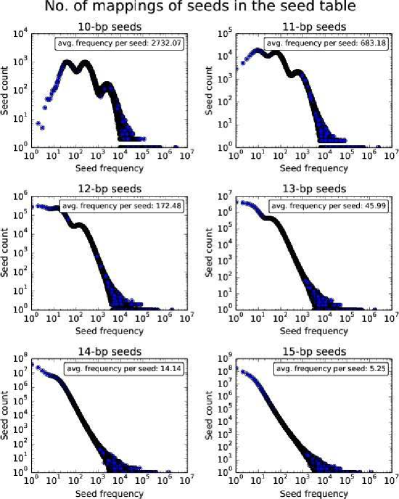
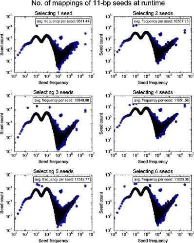
From Figure 1, we can also observe that the frequencies of seeds are not evenly distributed: for seeds with lengths between 10 to 15 base-pairs, many seeds have frequencies below 100, as in the figure, seed frequencies below 100 have high seed counts, often over $10^{3}$. However, there are also a few seeds which have frequencies greater than 100K, even though the seed counts of such frequencies are very low, usually just $1$. This explains why most plots in Figure 1 follow a bimodal distribution; except for 10-bp seeds and perhaps 11-bp seeds, where the frequency of seeds peaks at around 100. Although ultra-frequent seeds (seeds that appear more frequently than $10^{4}$ times) are few among all seeds, they are ubiquitous in the genome. As a result, for a randomly selected read, there is a high chance that the read contains one or more of such frequent seeds. This effect is best illustrated in Figure 2, which presents the numbers of frequencies of consecutively selected seeds, when we map over 4 million randomly selected 101-bp reads from the 1000 Genome Project 1000GP to the human reference genome.

Figure 2: Frequency distribution of seeds at runtime by selecting 15-bp seeds consecutively while mapping 4,031,354 101-bp reads from a real read set, ERR240726 from the 1000 Genome Project, under different number of required seeds.

Unlike in Figure 1, in which the average frequency of 15-bp seeds is 5.25, the average frequencies of seeds in Figure 2 are all greater than 2.7K. Furthermore, from Figure 2, we can observe that the ultra-frequent seeds are selected far more often than some of the less frequent seeds, as the seed count increases with higher seed frequencies after $10^{4}$ (as opposed to Figure 1, where seed frequencies over $10^{4}$ usually have seed counts below $10$). This observation suggests that the ultra-frequent seeds are surprisingly numerous in reads, especially considering how few ultra-frequent seed patterns there are in total in the seed database (and the plots in Figure 2 no longer follow a bimodal distribution as in Figure 1). We call this phenomenon frequent seed phenomenon. Frequent seed phenomenon is explained in previous works Kielbasa2011 . To summarize, highly frequent seed patterns are ubiquitous in the genome, therefore they appear more often in randomly sampled reads, such as reads sampled from shotgun sequencing. Frequency distributions of other seed lengths are provided in the Supplementary Materials.

The key takeaway from Figure 1 and Figure 2 is that although longer seeds on average are less frequent than shorter seeds, some seeds are still much more frequent than others and are more prevalent in the reads. Therefore, with a naive seed selection mechanism (e.g., selecting seeds consecutively from a read), a mapper still selects many frequent seeds, which increases the number of calls to the computationally expensive verification process.

To reduce the total frequency of selected seeds, we need an intelligent seed selection mechanism to avoid using frequent patterns as seeds. More importantly, as there is a limited number of base-pairs in a read, we need to carefully choose the length of each seed. Extension of an infrequent seed does not necessarily provide much reduction in the total frequency of all seeds, but it will “consume” base-pairs that could have been used to extend other more frequent seeds. Besides determining individual seed lengths, we should also intelligently select the position of each seed. If multiple seeds are selected from a small region of the read, as they are closely packed together, seeds are forced to keep short lengths, which potentially increase their seed frequency.

Based on the above observations, our goal in this paper is to develop an algorithm that can calculate both the length and the placement of each seed in the read. Hence, the total frequency of all seeds will be minimized. We call such a set of seeds the optimal seeds of the read as they produce the minimum number of potential mappings to be verified while maintaining the sensitivity of the mapper. We call the sum of frequencies of the optimal seeds the optimal frequency of the read.

7 Methods

The biggest challenge in deriving the optimal seeds of a read is the large search space. If we allow a seed to be selected from an arbitrary location in the read with an arbitrary length, then from a read of length $L$, there can be $\frac{L\times(L+1)}{2}$ possibilities to extract a single seed. When there are multiple seeds, the search space grows exponentially since the position and length of each newly selected seed depend on positions and lengths of all previously selected seeds. For $x$ seeds, there can be as many as $\mathcal{O}(\frac{L^{2\times x}}{x!})$ seed selection schemes.

Below we propose Optimal Seed Solver (OSS), a dynamic programming algorithm that finds the optimal set of $x$ seeds of a read in $\mathcal{O}(x\times L)$ operations on average and in $\mathcal{O}(x\times L^{2})$ operations in the worst case scenario.

Although in theory a seed can have any length, in OSS, we assume the length of a seed is bounded by a range [$S_{min}$, $S_{max}$]. This bound is based on our observation that in practice, neither very short seeds nor very long seeds are commonly selected in optimal seeds. Ultra-short seeds ($<8$-bp) are too frequent. Most seeds shorter than 8-bp have frequencies over 1000. Ultra-long seeds “consume” too many base-pairs from the read, which shorten the lengths of other seeds and increase their frequencies. Furthermore, long seeds (e.g., 40-bp) are mostly either unique or non-existent in the reference genome (seed of 0 frequency is still useful in read mapping as it confirms there exist at least one error it). Extending a unique or non-existent seed longer provides little benefit while “consuming” extra base-pairs from the read.

Bounding seed lengths reduces the search space of optimal seeds. However, it is not essential to OSS. OSS can still work without seed length limitations (to lift the limitations, one can simply set $S_{min}=1$ and $S_{max}=L$), although OSS will perform extra computation.

Below we describe our Optimal Seed Solver algorithm in three sections. First, we introduce the core algorithm of OSS. Then we improve the algorithm with two optimizations, optimal divider cascading and early divider termination. Finally we explain the overall algorithm and provide the pseudo code.

7.1 The core algorithm

A naive brute-force solution to find the optimal seeds of a read would be systematically iterating through all possible combinations of seeds. We start with selecting the first seed by instantiating all possible positions and lengths of the seed. On top of each position and length of the first seed, we instantiate all possible positions and lengths of the second seed that is sampled after (to the right-hand side of) the first seed. We repeat this process for the rest of the seeds until we have sampled all seeds. For each combination of seeds, we calculate the total seed frequency and find the minimum total seed frequency among all combinations.

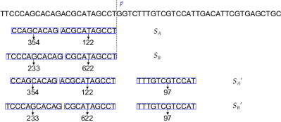
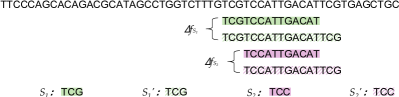
The key problem in the brute-force solution above is that it examines a lot of obviously suboptimal combinations. For example, in Figure 3, there are two $m$-seed combinations, $S_{A}$ and $S_{B}$, extracted from the same read, $R$. Both combinations end at the same position, $p$, in $R$. Among them, $S_{A}$ is more “optimal” than $S_{B}$ as it has a smaller total seed frequency. Then for any number of seeds that is greater than $m$, we know that in the final optimal solution of $R$, seeds before position $p$ will not be exactly like $S_{B}$, since any seeds that are appended after $S_{B}$ (e.g., $S_{B}^{\prime}$ in Figure 3) can also be appended after $S_{A}$ (e.g., $S_{A}^{\prime}$ in Figure 3) and produce a smaller total seed frequency. In other words, compared to $S_{B}$, only $S_{A}$ has the potential to be part of the optimal solution and worth appending more seeds after. In general, among two combinations that have equal numbers of seeds and end at the same position in the read, only the combination with the smaller total seed frequency has the potential of becoming part of a bigger (more seeds) optimal solution. Therefore, for a partial read and all combinations of a subset set of seeds in this partial read, only the optimal subset of seeds of this partial read (with regard to different numbers of seeds) might be relevant to the optimal solution of the entire read. Any other suboptimal solutions of this partial read (with regard to different numbers of seeds) will not lead to the optimal solution and should be pruned.

Figure 3: Two 2-seed combinations, $S_{A}$ and $S_{B}$ that end at the same position, $p$, in the read. The total seed frequency of $S_{A}$ is smaller than $S_{B}$. Both combinations can be extended by adding a third seed, making them $S_{A}^{\prime}$ and $S_{B}^{\prime}$ respectively. For any third seed, the total seed frequency of $S_{B}^{\prime}$ must be greater than $S_{A}^{\prime}$. Hence, $S_{B}$ must not be part of any optimal solution.

The above observation suggests that by summarizing the optimal solutions of partial reads under a smaller number of seeds, we can prune the search space of the optimal solution. Specifically, given $m$ (with $m<x$) seeds and a substring $U$ that starts from the beginning of the read, only the optimal $m$ seeds of $U$ could be part of the optimal solution of the read. Any other suboptimal combinations of $m$ seeds of $U$ should be pruned.

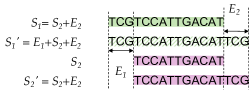
Storing the optimal solutions of partial reads under a smaller number of seeds also helps speed up the computation of larger numbers of seeds. Assuming we have already calculated and stored optimal the optimal frequency of $m$ seeds of all substrings of $R$, to calculate the optimal $(m+1)$-seed solution of a substrings, we can iterate through a series of divisions of this substring. In each division, we divide the substring into two parts: We extract $m$ seeds from the first part and 1 seed from the second part. The minimum total seed frequency of this division (or simply the “optimal frequency of the division”) is simply the sum of the optimal $m$-seed frequency of the first part and the optimal 1-seed frequency of the second part. As we already have both the optimal $m$-seed frequency of the first part and the 1-seed frequency of the second part calculated and stored, the optimal frequency of this division can be computed with one addition and two lookups.

The optimal $(m+1)$-seed solution of this substring is simply the division that yields the minimum total frequency. Given that each seed requires at least $S_{min}$ base-pairs, for a substring of length $L^{\prime}$, there are in total $L^{\prime}-(m+1)\times S_{min}$ possible divisions to be examined. This relationship can be summarized as a recurrence function in Equation 1, in which $Opt(U,m)$ denotes the optimal $m$-seed frequency of substring $U$ and $u$ denotes the length of $U$.

$$Opt(U,m+1)=\min_{i}Opt(R[1:i-1],m)+Opt(R[i:u],1)$$ (1)

OSS implements the above strategy using a dynamic programming algorithm: To calculate the optimal $(x+1)$-seed solution of a read, $R$, OSS computes and stores optimal solutions of partial reads with fewer seeds through $x$ iterations. In each iteration, OSS computes optimal solutions of substrings with regard to a specific number of seeds. In the $m^{th}$ iteration ($m\leq x$), OSS computes the optimal $m$-seed solutions of all substrings that starts from the beginning of $R$, by re-using optimal solutions computed from the previous $(m-1)^{th}$ iteration. For each substring, OSS performs a series of divisions and finds the division that provides the minimum total frequency of $m$ seeds. For each division, OSS computes the optimal $m$-seed frequency by summing up the optimal $(m-1)$-seed frequency of the first part and the 1-seed frequency of the second part. Both frequencies can be obtained from previous iterations. Overall, OSS starts from 1 seed and iterates to $x$ seeds. Finally OSS computes the optimal $(x+1)$-seed solution of $R$ by finding the optimal division of $R$ and reuses results from the $x^{th}$ iteration.

7.2 Further optimizations

With the dynamic programming algorithm, OSS can find the optimal $(x+1)$ seeds of a $L$-bp read in $\mathcal{O}(x\times L^{2})$ operations: In each iteration, OSS examines $\mathcal{O}(L)$ substrings $(L-i\times S_{min}$ substrings for the $i^{th}$ iteration$)$ and for each substring OSS inspects $\mathcal{O}(L)$ divisions $(L^{\prime}-i\times S_{min}$ divisions of a $L^{\prime}$-bp substring$)$. In total, there are $\mathcal{O}(L^{2})$ divisions to be verified in an iteration.

To further speed up OSS and reduce the average complexity of processing each iteration, we propose two optimizations to OSS: optimal divider cascading and early divider termination. With both optimizations, we empirically reduce the average complexity of processing an iteration to $\mathcal{O}(L)$. Below we describe both optimizations in detail.

7.2.1 Optimal divider cascading

Until this point, our assumption is that optimal solutions of substrings within an iteration are independent from each other: the optimal division (the division that provides the optimal frequency of the substring) of one substring is independent from the optimal division of another substring, thus they must be derived independently.

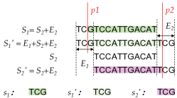
We observe that this assumption is not necessarily true as there exists a relationship between two substrings of different lengths in the same iteration (under the same seed number): the first optimal divider (the optimal divider that is the closest towards the beginning of the read, if there exist multiple optimal divisions with the same total frequency) of the shorter substring must be at the same or a closer position towards the beginning of the read, compared to the first optimal divider of the longer substring. We call this phenomenon the optimal divider cascading, and it is depicted in Figure 4. The proof that the optimal divider cascading is always true is provided in the Supplementary Materials.

Figure 4: All substrings and their first optimal dividers in an iteration. We observe that the first optimal divider of a longer substring is never more towards the beginning of the read than the first optimal divider of a shorter substring.

Based on the optimal divider cascading phenomenon, we know that for two substrings in the same iteration, the first optimal divider of the shorter substring must be no further than the first optimal divider of the longer substring. With this relationship, we can reduce the search space of optimal dividers in each substring by processing substrings within an iteration from the longest to the shortest.

In each iteration, we start with the longest substring of the read, which is the read itself. We examine all divisions of the read and find the first optimal divider of it. Then, we move to the next substring of the length $|L-1|$. In this substring, we only need to check dividers that are at the same or a prior position than the first optimal divider of the read. After processing the length $|L-1|$ substring, we move to the length $|L-2|$ substring, whose search space is further reduced to positions that are at the same or a closer position to the beginning of the read than the first optimal divider of the length $|L-1|$ substring. This procedure is repeated until the shortest substring in this iteration is processed.

7.2.2 Early divider termination

With optimal divider cascading, we are able to reduce the search space of the first optimal divider of a substring and exclude positions that come after the first optimal divider of the previous, 1-bp longer substring. However, the search space is still large since any divider prior to the first optimal divider of the previous substring could be the optimal divider. To further reduce the search space of dividers in a substring, we propose the second optimization – early divider termination.

The key idea of early divider termination is simple: The optimal frequency of a substring monotonically non-increases as the substring extends longer in the read (see Lemma 1 in Supplementary Materials for the proof of this fact).

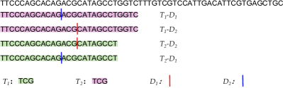
Based on the optimal divider cascading, we start at the position of the first optimal divider in the previous substring. Then, we gradually move the divider towards the beginning (or simply moving backward) and check the total seed frequency of the division after each move. During this process, the first part of the division gradually shrinks while the second part gradually grows, as we show in Figure 5. According to the Lemma 1 in the Supplementary Materials, the optimal frequency of the first part must be monotonically non-decreasing while the optimal frequency of the second part must be monotonically non-increasing.

Figure 5: Propagating dividers in a substring. The divider starts at the position of the previous substring’s first optimal divider, then gradually moves towards the beginning of the substring, until it reaches the termination position, $T$.

For each position of the divider, let $\mathtt{FREQ}_{P_{2}}$ denote the frequency of the second part $(P_{2})$ and $\Delta\mathtt{FREQ}_{P_{1}}$ denote the change of frequency of the first part $(P_{1})$ between current and the next move. Early divider termination suggests that: the divider should stop moving backward, whenever $|\Delta\mathtt{FREQ}_{P_{1}}|>|\mathtt{FREQ}_{P_{2}}|$. All dividers that are prior to this position are guaranteed to have greater total seed frequencies. We call this stopping position the termination position, and the division at this position – termination division, denoted as $T$. We name the first and the second part of $T$ as $T_{1}$ and $T_{2}$ respectively.

For any divider that comes prior to the termination position, compared to the termination division, its first part is shorter and its second part is longer. Hence the optimal frequency of its first part is greater and the optimal frequency of its second part is smaller. Let $|\Delta\mathtt{FREQ}_{P_{1}^{\prime}}(T)|$ denote the increase of the optimal frequency of the first part between current division and termination division and $|\Delta\mathtt{FREQ}_{P_{2}^{\prime}}(T)|$ denote the decrease of the second part. Based on Lemma 1, we have $|\Delta\mathtt{FREQ}_{P_{1}^{\prime}}(T)|\geq|\Delta\mathtt{FREQ}_{T_{1}}|$. Since the frequency of a seed can be no smaller than 0, we also have $|\mathtt{FREQ}_{T_{2}}|\geq|\Delta\mathtt{FREQ}_{P_{2}^{\prime}}(T)|$. Combining the three inequalities, we have $|\Delta\mathtt{FREQ}_{P_{1}}(T)|>|\Delta\mathtt{FREQ}_{P_{1}}(T)|$. This suggests that compared to the termination division, the frequency increase of the first part must be greater than the frequency reduction of the second part. Hence, the overall optimal frequency of such division must be greater than the optimal frequency of the termination division. Therefore divisions prior to termination position cannot be optimal.

Using early divider termination, we can further reduce the search space of dividers within a substring and exclude all positions that are prior to the termination position. Since the second part of the substring hosts only one seed and frequencies of most seeds decrease to 1 after extending it to a length of over 20 bp, we observe that the termination position of a substring is reached fairly quickly, only after a few moves. With both optimal divider cascading and early divider termination, from our experiments, we observe that we only need to verify 5.4 divisions on average for each substring. To conclude, with both optimizations, we have reduced the average complexity of Optimal Seed Solver to $\mathcal{O}(x\times L)$.

7.3 The full algorithm

Below we present the full algorithm of Optimal Seed Solver. Before calculating the optimal $x$-seed frequency of the read, $R$, we assume that we already have the optimal 1-seed frequency of any substring of $R$ and it can be retrieved in a $\mathcal{O}(1)$-time lookup via the $optimalFreq(\mathrm{substring})$ function. This information can be pre-processed prior to mapping, or it can be calculated dynamically at runtime. If calculated at runtime, it requires at most $\mathcal{O}(L^{2})$ lookups to the seed database for all possible substrings of the read.

Let $firstOptDivider(\mathrm{substring})$ be the function to calculate the first optimal divider of a substring. Then the optimal set of seeds can be calculated by filling a 2-D array, $opt\_data$, of size $(x-1)\times L$. In this array, each element stores two data: an optimal seed frequency and a first optimal divider. For the element at $i^{th}$ row and $j^{th}$ column, it stores the optimal $i$-seed frequency of the substring $R[1...j]$ as well as the first optimal divider of the substring.

Input: the read, $\mathsf{R}$

Output: the optimal $x$-seed frequency of $\mathsf{R}$, $\mathsf{opt\_freq}$ and the first $x$-seed optimal divider of R, $\mathsf{opt\_div}$

Global data structure: the 2-D data array $\mathsf{opt\_data[\ ][\ ]}$

Functions:

$\mathit{firstOptDivider}$: computes the first optimal divider of the substring

$\mathit{optimalFreq}$: retrieves the optimal 1-seed frequency of a substring

Pseudocode:

// Fill the first iteration

for $\mathit{l}=L$ to $S_{min}$ do

       $\mathsf{substring}=\mathsf{R[\mathit{1...l}]}$;

       $\mathsf{opt\_data[\mathit{1}][\mathit{l}].freq}=\mathit{optimalFreq(\mathsf{substring})}$;

      

// From iteration 2 to x-1

for $\mathit{iter}=2$ to $x-1$ do

       // Previous optimal divider

       $\mathsf{prev\_div}=L-S_{min}+1$;

       for $\mathit{l}=L$ to $\mathit{iter}\times S_{min}$ do

             $\mathsf{substring}=\mathsf{R[1\mathit{...l}]}$;

             $\mathsf{div}=\mathit{firstOptDivider(\mathsf{substring},\mathit{iter},\mathsf{prev\_div})}$;

             $\mathsf{1st\_part}=\mathsf{R[1\mathit{...div}-1]}$;

             $\mathsf{2nd\_part}=\mathsf{R[\mathit{div...L}]}$;

             $\mathsf{1st\_freq}=\mathsf{opt\_data[\mathit{iter}-1][\mathit{div}-1].freq}$;

             $\mathsf{2nd\_freq}=\mathit{optimalFreq(\mathsf{2nd\_part})}$;

             $\mathsf{opt\_data[\mathit{iter}][\mathit{l}]}.div=\mathsf{div}$;

             $\mathsf{opt\_data[\mathit{iter}][\mathit{l}]}.freq=\mathsf{1st\_freq}+\mathsf{2nd\_freq}$;

             // optimal seed cascading

             $\mathsf{prev\_div}=\mathsf{div}$;

            

      

$\mathsf{prev\_div}=L-S_{min}+1$;

$\mathsf{opt\_div}=\mathit{firstOptDivider(\mathsf{R},L-S_{min}+1)}$;

$\mathsf{1st\_part}=\mathsf{R[1\mathit{...opt\_div}-1]}$;

$\mathsf{2nd\_part}=\mathsf{R[\mathit{opt\_div...L}]}$;

$\mathsf{1st\_freq}=\mathsf{opt\_data[\mathit{x}-1][\mathit{opt\_div}-1].freq}$;

$\mathsf{2nd\_freq}=\mathit{optimalFreq(\mathsf{2nd\_part})}$;

$\mathsf{opt\_freq}=\mathsf{1st\_freq}+\mathsf{2nd\_freq}$;

return $\mathsf{opt\_freq}$, $\mathsf{opt\_div}$;

Algorithm 1 optimalSeedSolver

Output: the first optimal divider of $\mathsf{substring}$, $\mathsf{opt\_div}$

Global data structure: the 2-D data array $\mathsf{opt\_data[\ ][\ ]}$

Functions:

$\mathit{optimalFreq}$: retrieves the optimal 1-seed frequency of a substring

Pseudocode:

$\mathsf{first\_div}=\mathsf{prev\_div}$;

$\mathsf{min\_freq}=\mathsf{MAX\_INT}$;

$\mathsf{prev\_1st\_freq}=\mathsf{MAX\_INT}$;

$\mathsf{prev\_2nd\_freq}=\mathsf{MAX\_INT}$;

for $\mathit{div}=\mathsf{prev\_div}$ to $(\mathit{iter}-1)\times S_{min}$ do

       $\mathsf{1st\_part}=\mathsf{substring[1\mathit{...div}-1]}$;

       $\mathsf{2nd\_part}=\mathsf{substring[\mathit{div...end}]}$;

       $\mathsf{1st\_freq}=\mathsf{opt\_data[\mathit{iter}][\mathit{div}-1].freq}$;

       $\mathsf{2nd\_freq}=\mathit{optimalFreq(\mathsf{2nd\_part})}$;

       // early divider termination

       if $(\mathsf{1st\_freq}-\mathsf{prev\_1st\_freq})>\mathsf{prev\_2nd\_freq}$ then

             $\mathit{break}$;

            

      $\mathsf{freq}=\mathsf{1st\_freq}+\mathsf{2nd\_freq}$;

       // update the optimal divider

       if $(\mathsf{freq}\leq\mathsf{min\_freq}$ then

             $\mathsf{min\_freq}=\mathsf{freq}$;

             $\mathsf{first\_div}=\mathsf{div}$;

            

      $\mathsf{prev\_1st\_freq}=\mathsf{1st\_freq}$;

       $\mathsf{prev\_2nd\_freq}=\mathsf{2nd\_freq}$;

      

return $\mathsf{first\_div}$;

Algorithm 2 firstOptDivider

Algorithm 1 provides the pseudo-code of $optimalSeedsFinder$ and Algorithm 2 provides the pseudo code of $firstOptDivider$.

To retrieve the starting and ending positions of each optimal seed, we can backtrack the 2-D array and backward induce the optimal substrings and their optimal dividers in each iteration. The pseudo code of the backtracking process is provided in Supplementary Materials.

8 Related Works

The primary contribution of this work is a dynamic programming algorithm that derives the optimal non-overlapping seeds of a read in $\mathcal{O}(x\times L)$ operations on average. To our knowledge, this is the first work that calculates the optimal seeds and the optimal frequency of a read. The most related prior works are optimizations to the seed selection mechanism which reduce the sum of seed frequencies of a read using greedy algorithms.

Existing seed selection optimizations can be classified into three categories: (1) extending seed length, (2) avoiding frequent seeds and (3) rebalancing frequencies among seeds. Optimizations in the first category extend frequent seeds longer in order to reduce their frequencies. Optimizations in the second category sample seed positions in the read and reject positions that generate frequent seeds. Optimizations in the third category rebalance frequencies among seeds such that the average seed frequency at runtime is more consistent with the static average seed frequency of the seed database.

We qualitatively compare the Optimal Seed Solver (OSS) to four representative prior works selected from the above three categories. They are: Cheap K-mer Selection (CKS) in FastHASH Xin2013 , Optimal Prefix Selection (OPS) in Hobbes hobbes , Adaptive Seeds Filter (ASF) in GEM mapper Marco-Sola2012 and spaced seeds in PatternHunter patternhunter . Among the four prior works, ASF represents works from the first category; CKS and OPS represent works from the second category and spaced seeds represents works from the third category. Below we elaborate each of them in greater details.

The Adaptive Seeds Filter (ASF) seeks to reduce the frequency of seeds by extending the lengths of the seeds. For a read, ASF starts the first seed at the very beginning of the read and keeps extending the seed until the seed frequency is below a pre-determined threshold, $t$. For each subsequent seed, ASF starts it from where the previous seed left off in the read, and repeats the extension process until the last seed is found. In this way, ASF guarantees that all seeds have a frequency below $t$.

Compared to OSS, ASF has two major drawbacks. First, it does not allow any flexibility in seed placement. Seeds are always selected consecutively, starting from the beginning of the read. Second, it sets a fixed frequency threshold $t$ for all reads.

Selecting seeds consecutively starting at the beginning of a read does not always produce infrequent seeds. Although most seeds that are longer than 20-bp are either unique or non-existent in the reference, there are a few seeds that are still more frequent than 100 occurrences even at 40-bp (e.g., all “A”s). With a small $S_{max}$ (e.g., $S_{max}\leq 40$) and a small $t$ ($t\leq 50$), ASF cannot not guarantee that all selected seeds are less frequent than $t$. This is because ASF cannot extend a seed more than $S_{max}$-bp, even if its frequency is still greater than $t$. If a seed starts at a position that yields a long and frequent seed, ASF will extend the seed to $S_{max}$ and accept a seed frequency that is still greater than $t$.

Setting a static $t$ for all reads further worsens the problem. Reads are drastically different. Some reads do not include any frequent short patterns (e.g., 10-bp patterns) while other reads have one to many highly frequent short patterns. Reads without frequent short patterns do not produce frequent seeds in ASF, unless $t$ is set to be very large (e.g., $\geq 10,000$) and as a result the selected seeds are very short (e.g., $\leq 8$-bp). Reads with many frequent short patterns have a high possibility of producing longer seeds under medium-sized or small $t$’s (e.g., $\leq 100$). For a batch of reads, if the global $t$ is set to a small number, reads with many frequent short patterns will have a high chance of producing many long seeds that the read does not have enough length to support. If $t$ is set to a large number, reads without any frequent short patterns will produce many short but still frequent seeds as ASF will stop extending a seed as soon as it is less frequent than $t$, even though the read affords longer and less frequent seeds.

	Optimal Seed Solver	ASF	CKS	OPS	Spaced seeds	naive
Empirical average case complexity	$\mathcal{O}(x\times L)$	$\mathcal{O}(x)$	$\mathcal{O}(x\times log\frac{L}{k})$	$\mathcal{O}(x\times L)$	$\mathcal{O}(x)$	$\mathcal{O}(x)$
Number of lookups	$\mathcal{O}(L^{2})$	$\mathcal{O}(x)$	$\mathcal{O}(\frac{L}{k})$	$\mathcal{O}(L)$	$\mathcal{O}(x)$	$\mathcal{O}(x)$

Table 1: An average case complexity and memory traffic comparison (measured by the number of seed-frequency lookups) of seed selection optimizations, including Optimal Seed Solver (OSS), Adaptive Seeds Filter (ASF), Cheap K-mer Selection (CKS), Optimal Prefix Selection (OPS), spaced seeds and naive (selecting fixed-length seeds consecutively). Note that only OSS has different empirical average case complexity and worst case complexity. The average case and worst case complexity of other optimizations are equal.

Cheap K-mer Selection (CKS) aims to reduce seed frequencies by selecting seeds from a wider potential seed pool. For a fixed seed length $k$, CKS samples $\lfloor\frac{L}{k}\rfloor$ seed positions consecutively in a read, with each position apart from another by $k$-bp. Among the $\lfloor\frac{L}{k}\rfloor$ positions, it selects $x$ seed positions that yield the least frequent seeds (assuming the mapper needs $x$ seeds). In this way, it avoids using positions that generate frequent seeds.

CKS has low overhead. In total, CKS only needs $\lfloor\frac{L}{k}\rfloor$ lookups for seed frequencies followed by a sort of $\lfloor\frac{L}{k}\rfloor$ seed frequencies. Although fast, CKS can only provide limited seed frequency reduction as it has a very limited pool to select seeds from. For instance, in a common mapping setting where the read length $L$ is 100-bp and seed length $k$ is 12, the read can be divided into at most $\lfloor\frac{100}{12}\rfloor=8$ positions. With only 8 potential positions to select from, CKS is forced to gradually select more frequent seeds under greater seed demands. To tolerate 5 errors in this read, CKS has to select 6 seeds out of 8 potential seed positions. This implies that CKS will select the 3rd most frequent seed out of 8 potential seeds. As we have shown in Figure 1, 12-bp seeds on average have a frequency over 172, and selecting the 3rd frequent position out of 8 potential seeds renders a high possibility of selecting a frequent seed which has a higher frequency than average.

Similar to CKS, Optimal Prefix Selection (OPS) also uses fixed length seeds. However, it allows a greater freedom of choosing seed positions. Unlike CKS, which only select seeds at positions that are a multiple of the seed length $k$, OPS allows seeds to be selected from any position in the read, as long as they do not overlap.

Resembling our optimal seed finding algorithm, the basis of OPS is also a dynamic programming algorithm that implements a simpler recurrence function. The major difference between OPS and OSS is that OPS does not need to derive the optimal length of each seed, as the seed length is fixed to $k$ bp. This reduces the search space of optimal seeds to a single dimension, which is only the seed placements. The worst case/average complexity of OPS is $\mathcal{O}(L\times x)$.

Compared to CKS, OPS is more complex and requires more seed frequency lookups. In return, OPS finds less frequent seeds, especially under large seed numbers. However, with a fixed seed length, OPS cannot further reduce the seed frequencies by extending the seeds longer.

Spaced seeds aim at rebalancing frequencies among patterns in the seed database by introducing a hash function that is guided by a user-defined bit-mask. Different patterns that are hashed into the same hash value are considered as a single “rebalanced seed”. By carefully designing the hashing function, which extracts base-pairs only at selected positions from a longer (e.g., 18-bp) pattern, spaced seeds can group up frequent long patterns with infrequent long patterns and merge them into the new “rebalanced seeds”, which have smaller frequency variations. At runtime, long raw seeds are selected consecutively in the reads, which are processed by the rebalancing hash function later.

Compared to OSS, spaced seeds has two disadvantages. First, the hash function cannot perfectly balance frequencies among all “rebalanced seeds”. After rebalancing, there is still a large disparity in seed frequency amongst seeds. Second, seed placement in spaced seeds is static, and does not accommodate for high frequency seeds. Therefore, positions that generate frequent seeds are not avoided which still give rise to the frequent seeds phenomenon (frequent seeds are encountered more frequently in the reads, if selected consecutively).

9 Results

In this section, we compare the average case complexity, memory traffic and effectiveness of OSS against the four prior studies, ASF, CKS, OPS and spaced seeds as well as the naive mechanism, which selects fixed seeds consecutively. Memory traffic is measured by the number of required seed frequency lookups to map a single read. The effectiveness of a seed selection scheme is measured by the average seed frequency of mapping 4,031,354 101-bp reads from a real read set, ERR240726 from the 1000 Genomes Project, under different numbers of seeds.

We do not measure the execution time of each mechanism because different seed selection optimizations are combined with different seed database implementations. CKS, OPS and spaced seeds use hash tables for short, fixed-length seeds while ASF and OSS employs slower but more memory efficient BWT and FM-index for longer, variant-length seeds. However, this combination is inter-changeable. CKS, OPS, and spaced seeds can also work well with BWT and FM-index and ASF and OSS can also be combined with a large hash-table, given sufficient memory space. Besides, different existing implementations have their unique seed database optimizations, which introduces more variations to the execution time. With the above reasons, we only compare the complexity and memory traffic of each seed selection scheme, without measuring their runtime performance.

We benchmark each seed optimization scheme with multiple configurations. We benchmark ASF with multiple frequency thresholds, 5, 10, 100, 500 and 1000. If a read fails to provide enough seeds in ASF, due to having many long seeds under small thresholds, the read will be processed again in CKS with a fixed seed length of 12-bp. We benchmark CKS, OPS and naive under three fixed seed lengths, 12, 13 and 14. We benchmark spaced seeds with the default bit-mask, “110100110010101111”, which hashes 18-bp long seeds into 11-bp long signatures.

All seed selection mechanisms are benchmarked using an in-house seed database, which supports variant seed lengths between $S_{min}=10$ and $S_{max}=30$.

Table 1 summarizes the average complexity and memory traffic of each seed selection optimization. From the table, we can observe that OSS requires the most seed frequency lookups ($\mathcal{O}(L^{2})$) with the worst average case complexity, ($\mathcal{O}(x\times L)$), which tied with OPS. Nonetheless, OSS is the most effective seed selection scheme as Figure 6 shows. Among all seed selection optimizations, OSS provides the largest frequency reduction of seeds on average, achieving a 3x larger frequency reduction compared to the second best seed selection scheme, OPS.

Figure 6: Average seed frequency comparison among Optimal Seed Solver (OSS), Adaptive Seeds Filter (ASF), Cheap K-mer Selection (CKS), Optimal Prefix Selection (OPS), spaced seeds and naive (selecting fixed length seeds consecutively). The results are gathered by mapping 4031354 101-bp reads from the read set ERR240726_1 from 1000 Genome Project under different numbers of seeds (for better accuracy and error tolerance). In each figure, a smaller average seed frequency indicates a more effective seed selection mechanism.

As shown in Figure 6, the average seed frequencies of OSS, CKS and OPS increase with more seeds. This is expected as there is less flexibility in seed placement with more seeds. For OSS, more seeds also means shorter average seed length, which also contributes to greater average seed frequencies. For ASF, average seed frequencies remains similar for three or fewer seeds. When there are more than three seeds, the average seed frequencies increase with more seeds. This is because up until three seeds, all reads have enough base-pairs to accommodate all seeds, since the maximum seed length is $S_{max}=30$. However, once beyond three seeds, reads start to fail in ASF (having insufficient base-pairs to accommodate all seeds) and the failed reads are passed to CKS instead. Therefore the increase after three seeds is mainly due to the increase in CKS. For $t=10$ with six seeds, we observe from our experiment that 66.4% of total reads fail ASF and are processed in CKS instead.

For CKS and OPS, the average seed frequency decreases with increasing seed length when the number of seeds is small (e.g., $<4$). When the number of seeds is large (e.g., $6$), it is not obvious if greater seed lengths provide smaller average seed frequencies. In fact, for 6 seeds, the average seed frequency of OPS rises slightly when we increase the seed length from 13 bp to 14 bp. This is because, for small numbers of seeds, the read has plenty of space to arrange and accommodate the slightly longer seeds. Therefore, in this case, longer seeds reduce the average seed frequency. However, for large numbers of seeds, even a small increase in seed length will significantly decrease the flexibility in seed arrangement. In this case, the frequency reduction of longer seeds is surpassed by the frequency increase of reduced flexibility in seed arrangement. Moreover, the benefit of having longer seeds diminishes with greater seed lengths. Many seeds are already infrequent at 12-bp. Extending the infrequent seeds longer does not introduce much reduction in the total seed frequency. This result corroborates the urge of enabling flexibility in both individual seed length and seed placements.

Overall, OSS provides the least frequent seeds on average, achieving a 3x larger frequency reduction than the second best seed selection schemes, OPS.

10 Discussion

As shown in the Results section, OSS requires $\mathcal{O}(L^{2})$ seed-frequency lookups in order to derive the optimal solution of a read. For a non-trivial seed database implementation such as BWT with FM-index, this can be a time consuming process. For reads that do not include any frequent short patterns, OSS can be an expensive procedure with little benefit, as simpler seed selection mechanisms can also produce low-frequency seeds. Therefore, when designing a mapper, OSS is best used in junction with other greedy seed selection algorithms. In such configuration, OSS will only be invoked when greedy seed selection algorithms fail to deliver infrequent seeds. However, such study is beyond the scope of this paper and will be explored in our future research.

The Optimal Seed Solver also revealed that there is still great potential in designing better greedy seed selection optimizations. From our experiment, we observe that the most effective greedy seed selection optimization still provides 3x more frequent seeds on average than optimal. Better greedy algorithms that provides less frequent seeds without a large number of database lookups will also be included in our future research.

11 Conclusion

Optimizing seed selection is an important problem in read mapping. The number of selected non-overlapping seeds defines the error tolerance of a mapper while the total frequency of all selected seeds determines the performance of the mapper. To build a fast while error tolerant mapper, it is essential to select a large number of non-overlapping seeds while keeping each seed as infrequent as possible. In this paper, we confirmed frequent seed phenomenon discovered in previous works Kielbasa2011 , which suggests that in a naive seed selection scheme, mappers tend to select frequent seeds from reads, even when using long seeds. To solve this problem, we proposed Optimal Seed Solver (OSS), a dynamic-programming algorithm that derives the optimal set of seeds from a read that has the minimum total frequency. We further improved OSS with two optimizations, optimal divider cascading and early seed termination. With both optimizations, we reduced the average-case complexity of OSS to $\mathcal{O}(x\times L)$, and achieved a $\mathcal{O}(x\times L^{2})$ worst-case complexity. We compared OSS to four prior studies, Adaptive Seeds Filter, Cheap K-mer Selection, Optimal Prefix Selection and spaced seeds and showed that OSS provided a 3-fold seed frequency reduction over the best previous seed selection scheme, Optimal Prefix Selection.

Funding

This study is supported by an NIH grant (HG006004) to C. Alkan and O. Mutlu, HG007104 to C. Kingsford) and a Marie Curie Career Integration Grant (PCIG-2011-303772) to C. Alkan under the Seventh Framework Programme. C. Alkan also acknowledges support from The Science Academy of Turkey, under the BAGEP program.

Figure 7: Frequency distribution of 10-bp seeds at runtime by selecting seed consecutively under different number of required seeds.

Figure 8: Frequency distribution of 11-bp seeds at runtime by selecting seed consecutively under different number of required seeds.

Figure 9: Frequency distribution of 12-bp seeds at runtime by selecting seed consecutively under different number of required seeds.

Figure 10: Frequency distribution of 13-bp seeds at runtime by selecting seed consecutively under different number of required seeds.

Figure 11: Frequency distribution of 14-bp seeds at runtime by selecting seed consecutively under different number of required seeds.

1 Supplementary Materials

1.1 Runtime frequency distributions of seeds under variant lengths

This section presents seed frequency distributions at runtime with regard to different seed lengths. The results are obtained by naively selecting different fixed-length seeds consecutively in the process of mapping 4,031,354 101-bp reads from a real read set, ERR240726, from the 1000 Genome Project.

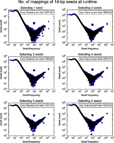
Figure 7 to Figure 11 from page 11-13 show seed frequency distributions of fixed-length seeds from 10-bp to 14-bp. From these figures, we have three observations: (1) the average seed frequencies of longer seeds are smaller, (2) beyond the seed frequency of $10^{4}$, more frequent seeds are more frequently selected at runtime and (3) compared to Figure 1, the average frequencies of selected seeds are much larger than the average frequencies of seeds with equal length in the seed database.

As shown in all five figures above, after $10^{4}$, the seed count increases with greater seed frequencies, which implies that frequent seeds are often selected from reads, regardless of the seed length.

1.2 Proof of optimal divider cascading

This section presents the detailed proof of the optimal divider cascading phenomenon.

The optimal divider cascading phenomenon can be explained with two lemmas:

Lemma 1.

For any two substrings from the same iteration in OSS, one substring must include the other. Among the two substrings, the minimum seed frequency of the outer substring must not be greater than the minimum seed frequency of the inner substring.

The proof of Lemma 1 is provided below:

Proof.

Since all substrings in the “Optimal Seed Solver” algorithm start at the beginning of the read, any two substrings from the same iteration must have one include another, as shown in Figure 4.

We prove the second part of the lemma using contradiction. Assume the outer substring has a greater optimal frequency (total seed frequency of the optimal seeds) than the inner substring. Because the inner substring is included by the outer substring, the optimal seeds of the inner substring are also valid seeds for the outer substring. Yet, the total frequency of this particular set of seeds is smaller than the optimal frequency of the outer substring, which leads to a contradiction. ∎∎

Lemma 2.

When extending two seeds of different lengths that end at the same position in the read by equal numbers of base-pairs, as one seed includes the other as shown in Figure 12, the frequency reduction ($\Delta f$) of extending the outer seed ($S_{2}\rightarrow S_{2}^{\prime}$) must not be greater than the frequency reduction of extending the inner seed ($S_{1}\rightarrow S_{1}^{\prime}$).

Figure 12: This figure shows two seeds $S_{1}$ and $S_{2}$, which are taken from the same read and end at the same position, with $S_{1}$ including $S_{2}$. Both seeds are extended by 3-bp into $S_{1}^{\prime}$ and $S_{2}^{\prime}$ respectively.

Lemma 2 can be proven with the monotonic non-increasing property of seed frequency with regard to a greater seed length. For example, in Figure 13, there are two seeds taken from the same read, $S_{1}$ and $S_{2}$, with $S_{1}$ including $S_{2}$ and both end at the same position in the read. Now, we simultaneously extend both $S_{1}$ and $S_{2}$ longer in the read (by taking more bp) by $3$ bp, into $S_{1}^{\prime}$ and $S_{2}^{\prime}$ respectively. With $\Delta f$ denoting the change of seed frequencies before and after extension, we can claim that $\Delta f_{S_{1}}\leq\Delta f_{S_{2}}$.

Figure 13: Two seeds, $S_{1}$ and $S_{2}$ are taken from the same read and end at the same position in the read. Both $S_{1}$ and $S_{2}$ are extended by 3 bp into $S_{1}^{\prime}$ and $S_{2}^{\prime}$ respectively. Considering $S_{1}$ as a left-extension of $S_{2}$ by $E_{1}$ and $S_{1}^{\prime}$ as a right-extension of $S_{1}$ by $E_{2}$, then we have $S_{1}=E_{1}+S_{2}+E_{2}$.

To prove this inequality, it is essential to understand how is $\Delta f$ calculated. As Figure 13 also shows, among the two seeds $S_{1}$ and $S_{2}$, $S_{1}$ can be considered as a “left-extension” of $S_{2}$. Therefore, $S_{1}$ can be represented as $S_{1}=E_{1}+S_{2}$, where $E_{1}$ denotes the left extension of $S_{1}$ and the “$+$” sign denotes a concatenation of strings. Similarly, $S_{1}^{\prime}$ can be represented as a “right-extension” of $S_{1}$, which can be also written as $S_{1}^{\prime}=E_{1}+S_{2}+E_{2}$, where $E_{2}$ is the right $m$-bp extension of $S_{1}$. By the same token, we also have $S_{2}^{\prime}=S_{2}+E_{2}$. If $\mathtt{freq}(S)$ denotes the frequency of a seed $S$, then $\Delta f_{S_{1}}=\mathtt{freq}(S_{1})-\mathtt{freq}(S_{1}^{\prime})=\mathtt{freq}(E_{1}+S_{2})-\mathtt{freq}(E_{1}+S_{2}+E_{2})$.

Below, we provide the proof of Lemma 2:

Proof.

If set $\overline{\mathbb{E}_{2}}$ denotes all DNA sequences that are equal in length with $E_{2}$ but excludes $E_{2}$ itself, which can be written as $\overline{\mathbb{E}_{2}}=\{s\;|\;(s\in\mathrm{DNA\ sequence})\wedge(|s|=|E_{2}|)\wedge(s\neq E_{2})\}$, then the reduced frequency of $S_{1}$ and $S_{2}$ can also be written as:

$$\Delta f_{S_{1}}=\sum_{s\in\overline{\mathbb{E}_{2}}}\mathtt{freq}(E_{1}+S_{2}+s)$$

$$\Delta f_{S_{2}}=\sum_{s\in\overline{\mathbb{E}_{2}}}\mathtt{freq}(S_{2}+s)$$

The right hand side of both equations denote the sum of frequencies of all seeds that share the same beginning sequence $E_{1}+S_{2}$ (or just $S_{2}$) other than the sequence $E_{1}+S_{2}+E_{2}$ itself (or $S_{2}+E_{2}$ for $S_{2}^{\prime}$), which is indeed $\mathtt{freq}(E_{1}+S_{2})-\mathtt{freq}(E_{1}+S_{2}+E_{2})$ (or $\mathtt{freq}(S_{2})-\mathtt{freq}(S_{2}+E_{2})$ for $S_{2}$).

From both equations, we can see that both $\Delta f_{S_{1}}$ and $\Delta f_{S_{2}}$ iterates through the same set of strings, $\overline{\mathbb{E}_{2}}$. For each string $i$ in set $\overline{\mathbb{E}_{2}}$, we have $\mathtt{freq}(E_{1}+S_{2}+i)\leq\mathtt{freq}(S_{2}+i)$, as the extended longer seed can only be less or equally frequent as the original shorter seed. Therefore, we have $\Delta f_{S_{1}}\leq\Delta f_{S_{2}}$. ∎∎

From Lemma 2, we can deduce Corollary 2.1:

Corollary 2.1.

When extending two substrings of different lengths that ends at the same position in the read by equal number of seeds, as one substring includes the other, the frequency reduction of the optimal seed (the optimal single seed) of extending the longer substring, is strictly not greater than the frequency reduction of the optimal seed of extending the shorter substring.

We prove Corollary 2.1 by cases:

Proof.

Considering the four substrings from Figure 13, $S_{1}$, $S_{2}$, $S_{1}^{\prime}$ and $S_{2}^{\prime}$. Among the four substrings, we have the following relationships:

$$\left\{\begin{array}[]{l}S_{1}=E_{1}+S_{2}\\ S_{1}^{\prime}=E_{1}+S_{2}+E_{2}\\ S_{2}^{\prime}=S_{2}+E_{2}\\ \end{array}\right.$$

There are in total three possible cases of where the optimal seed is selected in $S_{1}^{\prime}$: (1) it is selected from the region of $S_{2}+E_{2}$, (2) it is selected from the region $E_{1}+S_{2}$ and the optimal seed overlaps with $E_{1}$ and (3) it is selected from the region of $E_{1}+S_{2}+E_{2}$ and the seed overlaps with both $E_{1}$ and $E_{2}$. Below we prove that the Corollary is correct in each case.

Case 1: The optimal seeds is selected exclusively from $S_{2}+E_{2}$.

This suggests that the optimal seed in $S_{1}^{\prime}$ is also the optimal seed in $S_{2}^{\prime}$. Based on Lemma 1, we know the optimal frequency of $S_{1}$ is not greater than $S_{2}$.

Combining the two deductions above, we can conclude that extending $S_{2}$ to $S_{2}^{\prime}$ provides a strictly no smaller frequency reduction of the optimal seed than extending $S_{1}$ to $S_{1}^{\prime}$.

Case 2: The optimal seed is selected from the region $E_{1}+S_{2}$ and it overlaps with $E_{1}$.

Since the optimal seed does not overlap with $E_{2}$, the optimal seed in both $S_{1}$ and $S_{1}^{\prime}$ must be the same. Therefore extending $S_{1}$ to $S_{1}^{\prime}$ provides 0 frequency reduction of the optimal seed. As Lemma 1 suggests, the optimal seed frequency of $S_{2}$ must not be greater than the optimal seed frequency of $S_{2}^{\prime}$. As a result, the Corollary holds in this case.

Case 3: The optimal seed is selected across $E_{1}+S_{2}+E_{2}$ and it overlaps with both $E_{1}$ and $E_{2}$.

Assume the optimal seed, $s_{1}^{\prime}$, in $S_{1}^{\prime}$ starts at position $p_{1}$ and ends at position $p_{2}$. Assume a seed, $s_{1}$, which starts at $p_{1}$ but ends where $S_{1}$ ends, as shown in Figure 14. Also assume a seed, $s2^{\prime}$, which starts at where $S_{2}^{\prime}$ starts and ends at $p_{2}$. From Lemma 2, we know that the reduction of seed frequency of extending $s_{1}$ to $s_{1}^{\prime}$ is no greater than the seed frequency reduction of extending $S_{2}$ to $s_{2}^{\prime}$. We also know that the optimal seed frequency of $S_{1}$ is no greater than the seed frequency of $s_{1}$ and the optimal seed frequency of $S_{2}^{\prime}$ is no greater than the seed frequency of $s_{2}^{\prime}$. As a result, the frequency reduction of the optimal seed by extending $S_{1}$ to $S_{1}^{\prime}$, is strictly no greater than the frequency reduction of the optimal seed by extending $S_{2}$ to $S_{2}^{\prime}$. ∎∎

Figure 14: Among the four substrings, $S_{1}$, $S_{2}$, $S_{1}^{\prime}$ and $S_{2}^{\prime}$ from Figure 13, assume $s_{1}^{\prime}$ is the optimal seed of substring $S_{1}^{\prime}$. Also assume two new seeds, $s_{1}$ and $s_{2}^{\prime}$. Between the two seeds, $s_{1}$ starts at where $s_{1}^{\prime}$ starts but ends at where $S_{1}$ ends while $s_{2}^{\prime}$ starts at where $S_{2}^{\prime}$ starts and ends at where $s_{1}^{\prime}$ ends.

Using Lemma 1, Lemma 2 and Corollary 2.1, we are ready to prove that the optimal divider cascading phenomenon is always true.

Theorem 3.

For two substrings from the same iteration in OSS, as one substring includes the other, the first optimal divider of the outer substring must not be at the same or a prior position than the first optimal divider of the inner substring.

Theorem 3 can be proven by contradiction. The proof is provided below:

Proof.

Assume $T_{1}$ and $T_{2}$ are two substrings from the same iteration in “Optimal Seed Solver”, with $T_{1}$ including $T_{2}$. Also assume $T_{1}$’s first optimal divider, $D_{1}$, is closer to the beginning of the read than $T_{2}$’s first optimal divider, $D_{2}$, as shown in Figure 15 ($D_{1}<D_{2}$).

Figure 15: Two substring $T_{1}$ and $T_{2}$ taken from the same iteration. We assume $T_{1}$’s first optimal divider is at $D_{1}$ and $T_{2}$’s first optimal divider is at $D_{2}$.

Suppose we apply both divisions $D_{1}$ and $D_{2}$ to both substrings $T_{1}$ and $T_{2}$, which renders four divisions: $T_{1}$-$D_{1}$, $T_{1}$-$D_{2}$, $T_{2}$-$D_{1}$ and $T_{2}$-$D_{2}$, as Figure 15 shows. We can prove that $T_{2}$-$D_{2}$ is a strictly less frequent solution than $T_{2}$-$D_{1}$. Since $D_{2}$ is the first optimal divider of $T_{2}$ and $D_{1}<D_{2}$, the minimum frequency of dividing $T_{2}$ at $D_{1}$ must be greater than dividing $T_{2}$ at $D_{2}$. Let $\mathtt{freq}(T,D)$ denotes the optimal frequency of dividing substring $T$ at position $D$, then based on our assumptions and lemma 2, we have the following relationships:

$$\left\{\begin{array}[]{l}\mathtt{freq}(T_{1},D_{1})\leq\mathtt{freq}(T_{1},D_{2})\\ \mathtt{freq}(T_{2},D_{2})<\mathtt{freq}(T_{2},D_{1})\\ \mathtt{freq}(T_{1},D_{1})\geq\mathtt{freq}(T_{2},D_{1})\\ \mathtt{freq}(T_{1},D_{2})\geq\mathtt{freq}(T_{2},D_{2})\end{array}\right.$$

Based on corollary 2.1, we know that the frequency reduction of extending $T_{2}$-$D_{1}$ to $T_{1}$-$D_{1}$ is strictly not greater than the frequency reduction of extending $T_{2}$-$D_{2}$ to $T_{1}$-$D_{2}$. From Figure 15, we can observe that only the second parts of both $T_{2}$-$D_{1}$ and $T_{2}$-$D_{2}$ are extended into $T_{1}$-$D_{1}$ and $T_{1}$-$D_{2}$ respectively. Between $T_{2}$-$D_{1}$ and $T_{2}$-$D_{2}$, we can see that $D_{1}$ produces a longer second part than $D_{2}$. Based on the corollary of lemma 3, the frequency reduction of extending $T_{2}$-$D_{2}$ to $T_{1}$-$D_{2}$ is no less than the frequency reduction of extending $T_{2}$-$D_{1}$ to $T_{1}$-$D_{1}$. Given that $\mathtt{freq}(T_{2},D_{2})<\mathtt{freq}(T_{2},D_{1})$ from above, we prove that $\mathtt{freq}(T_{1},D_{2})<\mathtt{freq}(T_{1},D_{1})$, which contradicts our assumption that $\mathtt{freq}(T_{1},D_{2})\geq\mathtt{freq}(T_{2},D_{2})$. Therefore, the first optimal divider of $T_{1}$ must not be at a prior position than the first optimal divider of $T_{2}$.

∎∎

1.3 Backtracking in Optimal Seed Solver

This section presents the pseudo code of the backtracking process in OSS.

Input: the final optimal divider of the read, $\mathsf{opt\_div}$

Output: an array of optimal dividers of the read, $\mathsf{div\_array}$

Global data structure: the 2-D data array $\mathsf{opt\_data[\ ][\ ]}$

Pseudocode:

// Push in the last divider

$\mathsf{div\_array.push(opt\_div)}$;

$\mathsf{prev\_div=opt\_div}$;

for $\mathit{iter}=x-1$ to $2$ do

       $\mathsf{div}=\mathsf{opt\_data[\mathit{iter}][\mathit{prev\_div-1}]}.div$;

       $\mathsf{div\_array.push(opt\_div)}$;

       $\mathsf{prev\_div=div}$;

      

return $\mathsf{div\_array}$;

Algorithm 3 Backtracking

The pseudo code of the backtracking process is provided in Algorithm 3. The key idea behind the backtracking algorithm is simple: In the element of the $i^{th}$ row and the $j^{th}$ column of $opt\_data$, stores the optimal divider, $div$, of the substring $R[1...j]$. This $div$ suggests that by optimally selecting $i-1$ seeds from $R[1...div-1]$ and one seed from $R[div...j]$, we can obtain the least frequent $i$ seeds from $R[1...j]$. From $div$ we can learn that substring $R[div...j]$ provides the $i^{th}$ optimal seeds. Similarly, by repeating this process for the element of $opt\_data[i-1][div-1]$, we can learn the position and length of the $(i$-$1)^{th}$ optimal seeds. We can repeat this process until we have learnt all optimal dividers of the read.

References

- (1) 1000 Genomes Project Consortium. A map of human genome variation from population-scale sequencing. Nature, 467:1061–1073, 2010.
- (2) 1000 Genomes Project Consortium. An integrated map of genetic variation from 1,092 human genomes. Nature, 491(7422):56–65, Nov 2012.
- (3) A. Ahmadi, A. Behm, N. Honnalli, C. Li, L. Weng, and X. Xie. Hobbes: optimized gram-based methods for efficient read alignment. Nucleic Acids Research, 40:e41, 2011.
- (4) C. Alkan, J. M. Kidd, T. Marques-Bonet, G. Aksay, F. Antonacci, F. Hormozdiari, J. O. Kitzman, C. Baker, M. Malig, O. Mutlu, S. C. Sahinalp, R. A. Gibbs, and E. E. Eichler. Personalized copy number and segmental duplication maps using next-generation sequencing. Nat Genet, 41:1061–1067, 2009.
- (5) M. Burrows, D. J. Wheeler, M. Burrows, and D. J. Wheeler. A block-sorting lossless data compression algorithm. 1994.
- (6) P. Ferragina and G. Manzini. Opportunistic data structures with applications. In Proceedings of the 41st Annual Symposium on Foundations of Computer Science, FOCS ’00, pages 390–, Washington, DC, USA, 2000. IEEE Computer Society.
- (7) J. Flannick, G. Thorleifsson, N. L. Beer, S. B. R. Jacobs, N. Grarup, N. P. Burtt, A. Mahajan, C. Fuchsberger, G. Atzmon, R. Benediktsson, J. Blangero, D. W. Bowden, I. Brandslund, J. Brosnan, F. Burslem, J. Chambers, Y. S. Cho, C. Christensen, D. A. Douglas, R. Duggirala, Z. Dymek, Y. Farjoun, T. Fennell, P. Fontanillas, T. Forsén, S. Gabriel, B. Glaser, D. F. Gudbjartsson, C. Hanis, T. Hansen, A. B. Hreidarsson, K. Hveem, E. Ingelsson, B. Isomaa, S. Johansson, T. Jørgensen, M. E. Jørgensen, S. Kathiresan, A. Kong, J. Kooner, J. Kravic, M. Laakso, J.-Y. Lee, L. Lind, C. M. Lindgren, A. Linneberg, G. Masson, T. Meitinger, K. L. Mohlke, A. Molven, A. P. Morris, S. Potluri, R. Rauramaa, R. Ribel-Madsen, A.-M. Richard, T. Rolph, V. Salomaa, A. V. Segrè, H. Skärstrand, V. Steinthorsdottir, H. M. Stringham, P. Sulem, E. S. Tai, Y. Y. Teo, T. Teslovich, U. Thorsteinsdottir, J. K. Trimmer, T. Tuomi, J. Tuomilehto, F. Vaziri-Sani, B. F. Voight, J. G. Wilson, M. Boehnke, M. I. McCarthy, P. R. Njølstad, O. Pedersen, G.-T. C. , T.-G. E. N. E. S. C. , L. Groop, D. R. Cox, K. Stefansson, and D. Altshuler. Loss-of-function mutations in SLC30A8 protect against type 2 diabetes. Nature Genetics, 46(4):357–363, Apr 2014.
- (8) P. Flicek and E. Birney. Sense from sequence reads: methods for alignment and assembly. Nature methods, 6(11 Suppl):S6–S12, Nov. 2009.
- (9) R. E. Green, J. Krause, A. W. Briggs, T. Maricic, U. Stenzel, M. Kircher, N. Patterson, H. Li, W. Zhai, M. H.-Y. Fritz, N. F. Hansen, E. Y. Durand, A.-S. Malaspinas, J. D. Jensen, T. Marques-Bonet, C. Alkan, K. Pr fer, M. Meyer, H. A. Burbano, J. M. Good, R. Schultz, A. Aximu-Petri, A. Butthof, B. H ber, B. H ffner, M. Siegemund, A. Weihmann, C. Nusbaum, E. S. Lander, C. Russ, et al. A draft sequence of the Neandertal genome. Science, 328:710–722, 2010.
- (10) S. Kiełbasa, R. Wan, K. Sato, P. Horton, and M. C. Frith. Adaptive seeds tame genomic sequence comparison. Genome Research, 21(3):487–493, 2011.
- (11) B. Ma, J. Tromp, and M. Li. Patternhunter: faster and more sensitive homology search. Bioinformatics, 18:440–445, 2002.
- (12) S. Marco-Sola, M. Sammeth, R. Guig , and P. Ribeca. The gem mapper: fast, accurate and versatile alignment by filtration. Nat Methods, 9(12):1185–1188, 2012.
- (13) T. Marques-Bonet, J. M. Kidd, M. Ventura, T. A. Graves, Z. Cheng, L. W. Hillier, Z. Jiang, C. Baker, R. Malfavon-Borja, L. A. Fulton, C. Alkan, G. Aksay, S. Girirajan, P. Siswara, L. Chen, M. F. Cardone, A. Navarro, E. R. Mardis, R. K. Wilson, and E. E. Eichler. A burst of segmental duplications in the genome of the African great ape ancestor. Nature, 457:877–881, 2009.
- (14) M. Meyer, M. Kircher, M.-T. Gansauge, H. Li, F. Racimo, S. Mallick, J. G. Schraiber, F. Jay, K. Prüfer, C. de Filippo, P. H. Sudmant, C. Alkan, Q. Fu, R. Do, N. Rohland, A. Tandon, M. Siebauer, R. E. Green, K. Bryc, A. W. Briggs, U. Stenzel, J. Dabney, J. Shendure, J. Kitzman, M. F. Hammer, M. V. Shunkov, A. P. Derevianko, N. Patterson, A. M. Andrés, E. E. Eichler, M. Slatkin, D. Reich, J. Kelso, and S. Pääbo. A high-coverage genome sequence from an archaic Denisovan individual. Science, 338(6104):222–226, Oct 2012.
- (15) G. Myers. A fast bit-vector algorithm for approximate string matching based on dynamic programming. J. ACM, 46(3):395–415, 1999.
- (16) S. B. Needleman and C. D. Wunsch. A general method applicable to the search for similarities in the amino acid sequence of two proteins. Journal of Molecular Biology, 48:443–453, 1970.
- (17) S. B. Ng, A. W. Bigham, K. J. Buckingham, M. C. Hannibal, M. J. McMillin, H. I. Gildersleeve, A. E. Beck, H. K. Tabor, G. M. Cooper, H. C. Mefford, C. Lee, E. H. Turner, J. D. Smith, M. J. Rieder, K.-I. Yoshiura, N. Matsumoto, T. Ohta, N. Niikawa, D. A. Nickerson, M. J. Bamshad, and J. Shendure. Exome sequencing identifies MLL2 mutations as a cause of Kabuki syndrome. Nat Genet, 42(9):790–793, Sep 2010.
- (18) J. Prado-Martinez, P. H. Sudmant, J. M. Kidd, H. Li, J. L. Kelley, B. Lorente-Galdos, K. R. Veeramah, A. E. Woerner, T. D. O’Connor, G. Santpere, A. Cagan, C. Theunert, F. Casals, H. Laayouni, K. Munch, A. Hobolth, A. E. Halager, M. Malig, J. Hernandez-Rodriguez, I. Hernando-Herraez, K. Prüfer, M. Pybus, L. Johnstone, M. Lachmann, C. Alkan, D. Twigg, N. Petit, C. Baker, F. Hormozdiari, M. Fernandez-Callejo, M. Dabad, M. L. Wilson, L. Stevison, C. Camprubí, T. Carvalho, A. Ruiz-Herrera, L. Vives, M. Mele, T. Abello, I. Kondova, R. E. Bontrop, A. Pusey, F. Lankester, J. A. Kiyang, R. A. Bergl, E. Lonsdorf, S. Myers, M. Ventura, P. Gagneux, D. Comas, H. Siegismund, J. Blanc, L. Agueda-Calpena, M. Gut, L. Fulton, S. A. Tishkoff, J. C. Mullikin, R. K. Wilson, I. G. Gut, M. K. Gonder, O. A. Ryder, B. H. Hahn, A. Navarro, J. M. Akey, J. Bertranpetit, D. Reich, T. Mailund, M. H. Schierup, C. Hvilsom, A. M. Andrés, J. D. Wall, C. D. Bustamante, M. F. Hammer, E. E. Eichler, and T. Marques-Bonet. Great ape genetic diversity and population history. Nature, 499(7459):471–475, Jul 2013.
- (19) D. Reich, R. E. Green, M. Kircher, J. Krause, N. Patterson, E. Y. Durand, B. Viola, A. W. Briggs, U. Stenzel, P. L. F. Johnson, T. Maricic, J. M. Good, T. Marques-Bonet, C. Alkan, Q. Fu, S. Mallick, H. Li, M. Meyer, E. E. Eichler, M. Stoneking, M. Richards, S. Talamo, M. V. Shunkov, A. P. Derevianko, J.-J. Hublin, J. Kelso, M. Slatkin, and S. P bo. Genetic history of an archaic hominin group from Denisova Cave in Siberia. Nature, 468:1053–1060, 2010.
- (20) T. Rognes. Faster smith-waterman database searches with inter-sequence simd parallelisation. BMC Bioinformatics, 12:221, 2011.
- (21) S. M. Rumble, P. Lacroute, A. V. Dalca, M. Fiume, A. Sidow, and M. Brudno. SHRiMP: Accurate mapping of short color-space reads. PLoS Comput Biol, 5:e1000386, 2009.
- (22) A. Scally, J. Y. Dutheil, L. W. Hillier, G. E. Jordan, I. Goodhead, J. Herrero, A. Hobolth, T. Lappalainen, T. Mailund, T. Marques-Bonet, S. McCarthy, S. H. Montgomery, P. C. Schwalie, Y. A. Tang, M. C. Ward, Y. Xue, B. Yngvadottir, C. Alkan, L. N. Andersen, Q. Ayub, E. V. Ball, K. Beal, B. J. Bradley, Y. Chen, C. M. Clee, S. Fitzgerald, T. A. Graves, Y. Gu, P. Heath, A. Heger, et al. Insights into hominid evolution from the gorilla genome sequence. Nature, 483:169–175, 2012.
- (23) T. F. Smith and M. S. Waterman. Identification of common molecular subsequences. Journal of Molecular Biology, 147:195–195, 1981.
- (24) A. Szalkowski, C. Ledergerber, P. Krahenbuhl, and C. Dessimoz. SWPS3 - fast multi-threaded vectorized Smith-Waterman for IBM Cell/B.e. and x86/SSE2. BMC Research Notes, 1(1):107+, 2008.
- (25) M. Ventura, C. R. Catacchio, C. Alkan, T. Marques-Bonet, S. Sajjadian, T. A. Graves, F. Hormozdiari, A. Navarro, M. Malig, C. Baker, C. Lee, E. H. Turner, L. Chen, J. M. Kidd, N. Archidiacono, J. Shendure, R. K. Wilson, and E. E. Eichler. Gorilla genome structural variation reveals evolutionary parallelisms with chimpanzee. Genome Res, 21:1640–1649, 2011.
- (26) D. Weese, M. Holtgrewe, and K. Reinert. RazerS 3: Faster, fully sensitive read mapping. Bioinformatics, 28(20):2592–2599, 2012.
- (27) H. Xin, J. Greth, J. Emmons, G. Pekhimenko, C. Kingsford, C. Alkan, and O. Mutlu. Shifted hamming distance: A fast and accurate simd-friendly filter to accelerate alignment verification in read mapping. Bioinformatics, Jan 2015.
- (28) H. Xin, D. Lee, F. Hormozdiari, S. Yedkar, O. Mutlu, and C. Alkan. Accelerating read mapping with FastHASH. BMC Genomics, 14(Suppl 1):S13, 2013.