SI-HEP-2015-07

QFET-2015-08

MITP/15-022

June 25, 2015

Angular Analysis of New Physics Operators
in polarized $\tau\to 3\ell$ Decays

Robin Brüser^a, Thorsten Feldmann^a, Björn O. Lange^a,
Thomas Mannel^a, Sascha Turczyk^b
a Theoretische Elementarteilchenphysik, Naturwissenschaftlich-technische Fakultät, Universität Siegen, 57068 Siegen, Germany

^b PRISMA Cluster of Excellence & Mainz Institute for Theoretical Physics,
Johannes Gutenberg University, 55099 Mainz, Germany

In a bottom-up approach we investigate lepton-flavour violating processes $\tau\to 3\ell$ that are mediated by New Physics encoded in effective-theory operators of dimension six. While the opportunity to scrutinize the underlying operator structure has been investigated before, we explore the benefits of utilising the polarization direction of the initial $\tau$ lepton and the angular distribution of the decay. Given the rarity of these events (if observed at all), we focus on integrated observables rather than spectra, such as partial rates and asymmetries. In an effort to estimate the number of events required to extract the coupling coefficients to the effective operators we perform a phenomenological study with virtual experiments.

1 Introduction

Within the Standard Model (SM) of particle physics, lepton flavour is conserved as long as the neutrino masses are exactly zero. The discovery of massive neutrinos and neutrino oscillations, however, shows that lepton flavour violation (LFV) is in principle allowed. For example the process $\tau^{-}\to\mu^{-}\gamma$ can occur at the one-loop level if a tau-neutrino oscillates into a muon-neutrino within the loop that is supplemented with a charged vector boson. If this mechanism were the only source of LFV then the branching fractions of the $\tau^{-}\to\mu^{-}\ell^{+}\ell^{-}$ and $\tau^{-}\to e^{-}\ell^{+}\ell^{-}$ decay channels are non-zero, but tiny – $\mathcal{O}(10^{-45\pm 5})$ or thereabouts – and clearly unobservable. Many New Physics (NP) scenarios, however, predict much higher branching fractions, very roughly $\mathcal{O}(10^{-10})$, which are at the edge of observability (see e.g. the review in [1]). Here and below $\ell$ denotes either a muon or an electron.

If such a decay were to be discovered (see e.g. [2]), as is not unrealistic given the hints on deviations from the SM in the lepton sector with the recent measurements of $R_{K}=\mathcal{B}(B\to K\mu^{+}\mu^{-})/\mathcal{B}(B\to Ke^{+}e^{-})$ by the LHCb collaboration [3] and the LFV Higgs decay $\mathcal{B}(h\to\mu\tau)=(0.89^{+0.40}_{-0.37})\%$ by the CMS experiment [4], it will be highly interesting to investigate the underlying interaction structure in order to disentangle possible NP models. In this paper we employ a bottom-up approach and treat the SM as an effective field theory, i.e. we consider higher-dimensional operators that consist only of SM fields and respect SM symmetries. Our aim is to gain qualitative and quantitative information on the couplings of these operators. It is obvious that such an approach will allow us to only gain direct insight into the couplings at the low scale – set by the tau-lepton mass – and not at the high scale of the responsible NP mechanisms. The implementation of the renormalization-group running of the couplings, which has been derived at one-loop level in [7, 5, 6], is beyond the scope of the current paper.

As some of us have shown in a previous publication [8], the $\tau\to 3\ell$ decays are mediated by a handful of dimension-6 operators with possibly complex coefficients. In that publication a Dalitz-plot analysis was entertained in order to differentiate between radiative and leptonic operators. Clearly, a reconstruction of a Dalitz distribution requires a large data sample which obviously is hard to obtain for a very rare, lepton number violating decay. Thus, in order to obtain information on the type of operator that mediates the decay and on the helicity structure of the interaction, appropriate observables need to be defined. Obvious candidates are observables such as forward-backward asymmetries, which can be measured even at very low statistics. Our strategy is therefore to define observables of partially integrated phase space, which can be measured by a simple counting experiment.

Additional information on the structure of the interaction can be gained by studying the decay of polarized tau leptons [9]. Such a polarization can be realized at $e^{+}e^{-}$ colliders [10] running close to the $\tau^{+}\tau^{-}$ threshold with polarized electrons or electrons and positrons. As we shall show in this paper, taking into account the spin direction of the decaying tau lepton allows us to obtain information on the structure of the interaction, even with quite small data samples.

The idea of using polarized tau leptons has also been discussed in [11], however, in the context of a specific NP model. Our focus is a general analysis in order to pin down the structure of the relevant interaction.

Considering the possible LFV tau decays into leptons one may classify the six distinct channels as (a) $\tau^{-}\to\ell^{-}\ell^{-}\ell^{+}$ with $\ell=\mu,e$, or (b) $\tau^{-}\to\mu^{-}e^{-}e^{+},\tau^{-}\to e^{-}\mu^{-}\mu^{+}$, or (c) $\tau^{-}\to e^{-}e^{-}\mu^{+},\tau^{-}\to\mu^{-}\mu^{-}e^{+}$. The processes in $(a)$ and $(c)$ involve identical particles in the final state, whereas $(b)$ does not. Radiative operators contribute to classes $(a)$ and $(b)$, but not $(c)$. For definiteness and simplicity we focus our attention solely on case $(a)$, in which two external mass scales suffice, the mass of the tau lepton, $m_{\tau}$, and the mass of the lighter lepton, $m$.

The paper is organised as follows: In the next section we define the effective Hamiltonian with open coefficients $\xi_{i}$, where $i$ counts through the various operators of mass-dimension 6. The setup of our calculation is described in detail, including the polarisation vector of the initial tau and the angles characterizing the position of the polarisation vector relative to the decay plane. As a result the totally differential decay rate is decomposed in terms of trigonometric functions of these angles. In chapter 3 we integrate the differential decay rate over the relevant parts of the phase space. The results are rather bulky in print, so we have diverted them to the appendix for easier reading. Chapter 4 consists of a phenomenological study of the two decay channels $\tau\to 3\mu$ and $\tau\to 3e$. The main question we try to answer is how well one could determine the Wilson coefficients of the dimension-6 operators under the hypothesis of having discovered a low number of events experimentally. We summarize in chapter 5.

2 Calculational framework

2.1 Operator basis

In the following, we adopt the conventions and notation of [8]. (For more details we also refer the reader to that reference.). Starting point is the most general set of dimension-six operators respecting the SM gauge symmetries (see [12, 13]). After integrating out the weak gauge bosons and the Higgs field after electroweak symmetry breaking, there remain four purely leptonic 4-fermion operators of dimension six. Ordering the operators by the chirality of the involved lepton fields, they can be expressed as

$$H^{(LL)(LL)}_{\rm lept} = \frac{g^{(LL)(LL)}_{V}}{\Lambda^{2}}(\bar{\ell}_{L}\gamma_{\mu}\tau_{L})(\bar{\ell}_{L}\gamma^{\mu}\ell_{L})\quad,\quad H^{(RR)(RR)}_{\rm lept}=\frac{g^{(RR)(RR)}_{V}}{\Lambda^{2}}(\bar{\ell}_{R}\gamma_{\mu}\tau_{R})(\bar{\ell}_{R}\gamma^{\mu}\ell_{R})\;,$$

$$H^{(LL)(RR)}_{\rm lept} = \frac{g^{(LL)(RR)}_{V}}{\Lambda^{2}}(\bar{\ell}_{L}\gamma_{\mu}\tau_{L})(\bar{\ell}_{R}\gamma^{\mu}\ell_{R})\quad,\quad H^{(RR)(LL)}_{\rm lept}=\frac{g^{(RR)(LL)}_{V}}{\Lambda^{2}}(\bar{\ell}_{R}\gamma_{\mu}\tau_{R})(\bar{\ell}_{L}\gamma^{\mu}\ell_{L})\;,$$ (1)

where we have already singled out the $\tau$-lepton fields. In this notation, the chirality structure $(LR)(RL)$ can be Fierz transformed to contribute to $H^{(LL)(RR)}_{\rm lept}$ and $H^{(RR)(LL)}_{\rm lept}$. Notice that in order to feed terms of the form $(LR)(LR)$, one would have to include dimension-eight operators in the SM effective field theory. Following [8], we assume that the NP scale $\Lambda$ is sufficiently large compared to the electroweak scale, that these contributions can be neglected (for similar reasoning in other context, see e.g. [14, 15]). In an explicit UV completion of the SM, the dimensionless couplings $g_{V}$ should be determined from a matching calculation.

Similarly, one generates radiative operators, where, at low energies, only couplings to the photon field have to be considered. (Contributions from intermediate $W^{\pm}$ or $Z^{0}$ bosons are already contained in (LABEL:eq:1).) We are then left with two more terms in the effective Hamiltonian,

$$H_{\rm rad}^{(LR)}=-\frac{e}{8\pi}\frac{v}{\Lambda^{2}}g_{\rm rad}^{(LR)}(\bar{\ell}_{L}\sigma_{\mu\nu}\tau_{R})F^{\mu\nu}\quad,\quad H_{\rm rad}^{(RL)}=-\frac{e}{8\pi}\frac{v}{\Lambda^{2}}g_{\rm rad}^{(RL)}(\bar{\ell}_{R}\sigma_{\mu\nu}\tau_{L})F^{\mu\nu}\;.$$

They contribute to the $\tau^{-}\to\ell^{-}\ell^{-}\ell^{+}$ amplitude via photon exchange, schematically

$$\langle\ell\ell\bar{\ell}|H_{\rm rad}^{(LR)}|\tau\rangle = \underbrace{\alpha_{\rm em}\frac{v}{\Lambda^{2}}g_{\rm rad}^{(LR)}}_{\xi_{5}m_{\tau}}\left(\bar{\ell}_{L}\frac{(-i)}{q^{2}}q^{\eta}\sigma_{\mu\eta}\tau_{R}\right)\left(\bar{\ell}\gamma^{\mu}\ell\right)\;,$$

$$\langle\ell\ell\bar{\ell}|H_{\rm rad}^{(RL)}|\tau\rangle = \underbrace{\alpha_{\rm em}\frac{v}{\Lambda^{2}}g_{\rm rad}^{(RL)}}_{\xi_{6}m_{\tau}}\left(\bar{\ell}_{R}\frac{(-i)}{q^{2}}q^{\eta}\sigma_{\mu\eta}\tau_{L}\right)\left(\bar{\ell}\gamma^{\mu}\ell\right)\;.$$ (3)

Here, for simplicity, we used the same notation for lepton fields and on-shell spinors, $q^{\mu}$ denotes the momentum flow through the virtual photon, and $\alpha_{\rm em}$ the usual electromagnetic fine-structure constant. In summary, the generic effective Hamiltonian for $\tau\to 3\ell$ decays can be written as

$$H_{\rm eff}=H^{(LL)(LL)}_{\rm lept}+H^{(RR)(RR)}_{\rm lept}+H^{(LL)(RR)}_{\rm lept}+H^{(RR)(LL)}_{\rm lept}+H_{\rm rad}^{(LR)}+H_{\rm rad}^{(RL)}\;.$$ (4)

For future convenience we shall combine the six couplings into a complex-valued vector

$$\xi^{T}=\left(\frac{g^{(LL)(LL)}_{V}}{\Lambda^{2}},\frac{g^{(RR)(RR)}_{V}}{\Lambda^{2}},\frac{g^{(LL)(RR)}_{V}}{\Lambda^{2}},\frac{g^{(RR)(LL)}_{V}}{\Lambda^{2}},\frac{\alpha_{\rm em}}{m_{\tau}}\frac{v}{\Lambda^{2}}g_{\rm rad}^{(LR)},\frac{\alpha_{\rm em}}{m_{\tau}}\frac{v}{\Lambda^{2}}g_{\rm rad}^{(RL)}\right)$$ (5)

of mass dimension (-2).

2.2 Spin polarization of the tau lepton

The spin polarization of a beam of particles is typically measured in the flight direction of said particles. In the setup of our calculation we will define the $z$-axis of our lab-frame coordinate system to be the flight direction of the tau lepton. The reference vector for the spin orientation is then chosen as $s^{\mu}=(0,0,0,1)$ in the tau lepton’s rest frame, with $s^{2}=-1$ and $s\cdot p_{\tau}=0$. In the calculation of the squared amplitude $|\mathcal{M}|^{2}$ we will then use the Dirac matrix

$$u^{\uparrow}\bar{u}^{\uparrow}=(\hbox to0.0pt{\hskip 0.56917pt/\hss}{p}_{\tau}+m_{\tau})\,\frac{1+\gamma_{5}\,\hbox to0.0pt{\hskip 0.56917pt/\hss}{s}}{2}$$ (6)

to project onto tau leptons with “spin-up”. In this way the spin vector $s^{\mu}$ only appears at most linearly in the squared amplitude. Note that there are then only three linearly independent invariants that one can build from $s^{\mu}$ and the lepton momenta in the decay $\tau^{-}(p_{\tau})\to\ell^{-}(p_{1})\,\ell^{-}(p_{2})\,\ell^{+}(p_{3})$. These can be taken as

$$t=s\cdot p_{2}\quad,\quad u=s\cdot p_{3}\quad,\quad v=\varepsilon_{\alpha\beta\gamma\delta}\ p_{\tau}^{\alpha}\,s^{\beta}\,p_{2}^{\gamma}\,p_{3}^{\delta}\;,$$ (7)

and therefore the squared amplitude of the spin-up tau decay can be decomposed as

$$|\mathcal{M}^{\uparrow}(p_{\tau},p_{1},p_{2},p_{3},s)|^{2} = g_{1}(p_{\tau},p_{1},p_{2},p_{3})+g_{t}(p_{\tau},p_{1},p_{2},p_{3})\,t$$ (8)

$$+g_{u}(p_{\tau},p_{1},p_{2},p_{3})\,u+g_{v}(p_{\tau},p_{1},p_{2},p_{3})\,v\;.$$

Similarly the decay of a “spin-down” polarized tau lepton can be calculated with the help of the projector $u^{\downarrow}\bar{u}^{\downarrow}=(\hbox to0.0pt{\hskip 0.56917pt/\hss}{p}_{\tau}+m_{\tau})(1-\gamma_{5}\hbox to0.0pt{\hskip 0.56917pt/\hss}{s})/2$. We stress that the direction in which the spin is measured, i.e. the $z$-axis (or reference vector $s^{\mu}$) remains fixed. With this point of view the variables defined in (7) remain unchanged when describing the decay of a spin-down rather than spin-up tau lepton. In this spin-down case one finds the same functions $g_{1,t,u,v}$ from above that describe the squared amplitude, albeit in the combination

$$|\mathcal{M}^{\downarrow}(p_{\tau},p_{1},p_{2},p_{3},s)|^{2} = g_{1}(p_{\tau},p_{1},p_{2},p_{3})-g_{t}(p_{\tau},p_{1},p_{2},p_{3})t$$ (9)

$$-g_{u}(p_{\tau},p_{1},p_{2},p_{3})u-g_{v}(p_{\tau},p_{1},p_{2},p_{3})v\;.$$

Therefore only the part $2g_{1}$ contributes to the unpolarized decay rate. The information contained in the functions $g_{t,u,v}$ would then be lost and could not be used in the effort to unveil the underlying operator structure. In what follows, we will use a slightly modified version of the decomposition (8) based on angles associated with these invariants.

2.3 Euler rotations

The three momenta $\vec{p}_{1},\vec{p}_{2},\vec{p}_{3}$ of the decay product span the decay plane. In general the spin direction $\vec{s}$ does not lie in this decay plane, and its orientation can be described with the help of two angles. For example, the angle between the normal of the decay plane and $\vec{s}$ is the first, and the angle between the momentum $p_{3}$ of the antilepton and the projection of $\vec{s}$ into the decay plane the second angle. For convenience we employ the technique of Euler rotations instead, which also serve to define the orientation of $\vec{s}$ and the decay plane:

We define the lab frame as the reference frame (RF) in which the tau lepton is at rest and the z-axis is aligned with the spin vector $\vec{s}=\vec{e}_{z}$. We will now perform rotations until this plane is spanned by the new basis vectors $\vec{e_{x}}^{\prime}$ and $\vec{e_{z}}^{\prime}$. Furthermore the antilepton’s momentum shall point directly in the $\vec{e_{z}}^{\prime}$ direction. This new RF is called the decay frame, or RF’. We define the following order of rotations to get from RF to RF’:

$$\vec{p_{1}}^{\prime}=R_{z}(\alpha)R_{y}(\beta)R_{z}(\gamma)\,\vec{p}_{1}\;,\quad\hbox{et cetera,}$$ (10)

with mathematically positive convention:

$$R_{z}(\alpha)=\left(\begin{array}[]{ccc}\cos\alpha&-\sin\alpha&0\\ \sin\alpha&\cos\alpha&0\\ 0&0&1\end{array}\right)\quad,\quad R_{y}(\beta)=\left(\begin{array}[]{ccc}\cos\beta&0&\sin\beta\\ 0&1&0\\ -\sin\beta&0&\cos\beta\end{array}\right)\;.$$ (11)

Hence the polarization direction vector in RF’ reads

$$\vec{s}^{\;\prime}=(\cos\alpha\,\sin\beta,\sin\alpha\,\sin\beta,\cos\beta)\;.$$ (12)

Note that there is no dependence on the first rotation angle $\gamma$, which reflects the azimuthal symmetry of the problem. The rotations are such that the decay plane coincides with the $x^{\prime}-z^{\prime}$ plane, so that we may parameterize

$$\vec{p_{1}}^{\prime}=-(\vec{p_{2}}^{\prime}+\vec{p_{3}}^{\prime})\quad,\quad\vec{p_{2}}^{\prime}=\left(\begin{array}[]{c}b_{2}\,\sin\varphi\\ 0\\ b_{2}\,\cos\varphi\end{array}\right)\quad,\quad\vec{p_{3}}^{\prime}=\left(\begin{array}[]{c}0\\ 0\\ b_{3}\end{array}\right)\;,$$ (13)

where the parameter $\varphi=\phi_{23}$ has a physical interpretation of the angle between $\vec{p}_{2}$ and $\vec{p}_{3}$ within the decay plane, which is independent of the rotation angles $\alpha,\beta,\gamma$. The lengths of the 3-vectors $b_{2}=|\vec{p_{2}}^{\prime}|=|\vec{p}_{2}|$ and similarly $b_{3}$ are expressed in terms of the energies $E_{i}$ as

$$b_{2}=\sqrt{E_{2}^{2}-m^{2}}\quad,\quad b_{3}=\sqrt{E_{3}^{2}-m^{2}}\quad,\quad\cos\phi_{23}=\frac{E_{1}^{2}-E_{2}^{2}-E_{3}^{2}+m^{2}}{2\sqrt{E_{2}^{2}-m^{2}}\sqrt{E_{3}^{2}-m^{2}}}\;.$$ (14)

While the momentum of the antilepton, $p_{3}$, is well defined, the lepton pair in the final state is indistinguishable if the leptons are of the same flavour, and we must be careful not to double count.

For the last Euler rotation, it is sufficient to consider values of $\alpha\in[0,\pi)$ to lock the decay plane into the $x^{\prime}-z^{\prime}$ plane. Therefore, in total we restrict the values of the rotation angles as

$$\alpha\in[0,\pi)\quad,\quad\beta\in[0,\pi)\quad,\quad\gamma\in[0,2\pi)\;.$$ (15)

Furthermore it is obvious that either $\vec{p_{1}}^{\prime}$ has a positive $x^{\prime}$ component and $\vec{p_{2}}^{\prime}$ a negative one, or the other way around. The parameter $\phi_{23}$ is well defined as the angle between $\vec{p}_{2}$ and $\vec{p}_{3}$ if we insist on naming that lepton’s momentum $\vec{p}_{2}$ which has a positive $x^{\prime}$ component, i.e.

$$\phi_{23}\in[0,\pi)\;.$$ (16)

(However, the squared amplitudes, which we are going to calculate, will be symmetric under the exchange of $p_{1}\leftrightarrow p_{2}$, as they must for identical particles in the final state.)
In terms of the angles and energies the invariants in (7) are

$$t = -b_{2}\sin\phi_{23}\cos\alpha\sin\beta-b_{2}\cos\phi_{23}\cos\beta\;,$$

$$u = -b_{3}\cos\beta\;,$$

$$v = -m_{\tau}b_{2}b_{3}\sin\phi_{23}\sin\alpha\sin\beta\;.$$ (17)

Therefore we may decompose the squared amplitude in (8) in terms of the trigonometric functions that appear above instead of the invariants themselves. Specifically we have
$$|\mathcal{M}^{\uparrow}|^{2}=J_{1}(E_{2},E_{3})+J_{2}(E_{2},E_{3})\cos\beta+J_{3}(E_{2},E_{3})\cos\alpha\sin\beta+J_{4}(E_{2},E_{3})\sin\alpha\sin\beta\;.$$ (18)

This setup allows us to quite easily pick out the individual contributions from $J_{1}$ to $J_{4}$ by folding the differential decay rate with appropriate weight functions.

2.4 Phase space

Besides the angles in (15) we choose two of the three energies of the final-state leptons, which in the rest frame of the tau satisfy $E_{1}+E_{2}+E_{3}=m_{\tau}$. It is a straight-forward exercise to show that the totally differential decay rate is then given by

$$\frac{d^{5}\Gamma(\tau^{\uparrow}\to 3\ell)}{d\alpha\,d\!\cos\beta\,d\gamma\,dE_{2}\,dE_{3}}=\frac{1}{2m_{\tau}}\frac{|\mathcal{M}^{\uparrow}|^{2}}{256\pi^{5}}\;.$$ (19)

Since $|\mathcal{M}^{\uparrow}|^{2}$ does not depend on the angle $\gamma$ one can trivially integrate over the allowed range. The phase space for the energies $E_{2}$ and $E_{3}$ is nearly triangular with edges that are smoothened out by the light-lepton mass $m$. One way of expressing the phase-space boundaries is, for example,

$$\frac{1}{2}(m_{\tau}-E_{2}-b_{2}d_{2})\leq E_{3}\,\leq\,\frac{1}{2}(m_{\tau}-E_{2}+b_{2}d_{2})\quad,\quad m\,\leq\,E_{2}\leq\,\frac{m_{\tau}^{2}-3m^{2}}{2m_{\tau}}\;,$$ (20)

where $b_{2}=\sqrt{E_{2}^{2}-m^{2}}$ as before, and

$$d_{2}=\frac{m_{\tau}^{2}-2m_{\tau}E_{2}-3m^{2}}{m_{\tau}^{2}-2m_{\tau}E_{2}+m^{2}}$$ (21)

is a function of $E_{2}$ that is near 1, except when $E_{2}$ is near the endpoint where $d_{2}$ rapidly falls to zero. Sometimes it is more advantageous to express these energies in Dalitz-like invariants $s_{ij}=(p_{i}+p_{j})^{2}$, for example when addressing the momentum flowing through the virtual photon in the radiative operators in (3). In terms of $s_{ij}$ the energies are

$$E_{2}=\frac{m_{\tau}^{2}+m^{2}-s_{13}}{2m_{\tau}}\quad,\quad E_{3}=\frac{m_{\tau}^{2}+m^{2}-s_{12}}{2m_{\tau}}\;.$$ (22)

For later reference we also state the phase-space region in which $\cos\phi_{23}\geq 0$, which is

$$\frac{1}{2}(m_{\tau}-E_{2}-b_{2}d_{2}) \leq E_{3}\leq \frac{m_{\tau}^{2}-2m_{\tau}E_{2}+m^{2}}{2(m_{\tau}-E_{2})}\;,$$

$$m \leq E_{2}\leq \frac{1}{2}(m_{\tau}-m)\;.$$ (23)

Similarly, for $\cos\phi_{12}\geq 0$, we have the restrictions

$$\frac{m_{\tau}(m_{\tau}-2E_{2})+2E_{2}^{2}-m^{2}}{2(m_{\tau}-E_{2})} \leq E_{3}\leq \frac{1}{2}(m_{\tau}-E_{2}+b_{2}d_{2})\;,$$

$$m \leq E_{2}\leq \frac{1}{2}(m_{\tau}-m)\;.$$ (24)

In Fig. 1 we show the phase space for all kinematically allowed values of $E_{2}$ and $E_{3}$ mentioned in equation (20) as well as for the regions defined by (2.4) and (2.4).

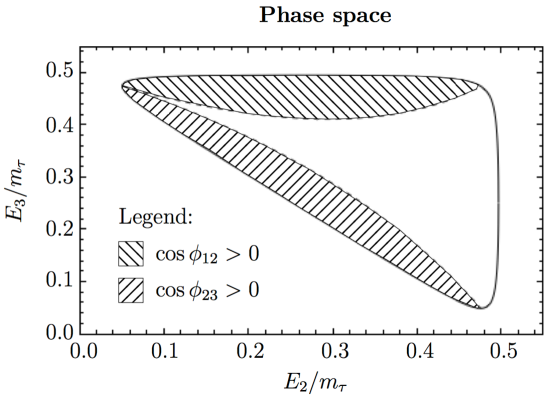
Figure 1: Available range of the energies $E_{2}$ and $E_{3}$. The shaded areas show the regions in which $\cos\phi_{23}>0$ and where $\cos\phi_{12}>0$.

3 Definition of the Observables

In this section we will use the formulae from the last chapter to define observables, which can be measured even with sparse data samples. All the observables will be defined from the coarsely sliced phase space using the angular variables, so that the observables correspond to partial rates and forward-backward asymmetries with respect to the angles, which also involve the direction of the tau-lepton polarization.

3.1 Coupling bilinears

Since lepton-flavour violating processes are rare, we focus on observables where the available phase space in $\alpha,\beta,E_{2},E_{3}$ is at least partially integrated. There are many such observables, and a measurement of them will allow us to draw conclusions on the underlying operator structures. We start by considering the integration of $J_{i}$ over the energies $E_{2}$ and $E_{3}$ in some region “R” of the phase space. The results are bilinears in the couplings $\xi$ in (5), and can be expressed in terms of $6\times 6$ hermitian matrices $\mbox{\boldmath$A$\unboldmath}_{i}^{\rm(R)}$ that depend on the region R, to wit

$$\iint\limits_{\rm R}dE_{2}\,dE_{3}\,J_{i}(E_{2},E_{3})=\frac{m_{\tau}^{6}}{6}\,\xi^{\dagger}\,\mbox{\boldmath$A$\unboldmath}_{i}^{\rm(R)}\,\xi\;.$$ (25)

From this notation it is obvious that the doubly differential decay rate in $\alpha,\beta$ is obtained by integration over the full energy phase space (20),

$$\frac{d^{2}\Gamma(\tau^{\uparrow}\to 3\ell)}{d\alpha\,d\!\cos\beta}=\frac{m_{\tau}^{5}}{6\cdot 256\pi^{4}}\xi^{\dagger}\Big{[}\mbox{\boldmath$A$\unboldmath}_{1}^{\rm\{full\}}+\mbox{\boldmath$A$\unboldmath}_{2}^{\rm\{full\}}\cos\beta+\mbox{\boldmath$A$\unboldmath}_{3}^{\rm\{full\}}\cos\alpha\sin\beta+\mbox{\boldmath$A$\unboldmath}_{4}^{\rm\{full\}}\sin\alpha\sin\beta\Big{]}\xi\;,$$ (26)

from which asymmetries using $\alpha,\beta$ are readily calculable. For example, the difference in the partial rates $\Gamma(\cos\beta>0)-\Gamma(\cos\beta<0)$ will only involve $\mbox{\boldmath$A$\unboldmath}_{2}^{\rm\{full\}}$. We may express this difference as the convolution integral over the differential decay rate (26) with the weight function $[\theta(\cos\beta)-\theta(-\cos\beta)]$, where $\theta$ is the Heaviside step function. In order to demonstrate that one can pick out each individual matrix using partial rates we note that

$$\int\limits_{0}^{\pi}d\alpha\int\limits_{-1}^{1}d\!\cos\beta\,\frac{d^{2}\Gamma}{d\alpha\,d\!\cos\beta}\,W(\alpha,\cos\beta)=\frac{m_{\tau}^{5}}{6\cdot 256\pi^{3}}\xi^{\dagger}\left[\sum\limits_{i=1}^{4}\tilde{c}_{i}\mbox{\boldmath$A$\unboldmath}_{i}^{\rm\{full\}}\right]\xi\;,$$ (27)

and list the coefficients $c_{i}$ for a few typical weight functions in Table 1. (Note the factor of $\pi$ that has been absorbed into the prefactor.)

Table 1: Coefficients of the linear combination in (27) for a few typical weight functions. Since the matrices $\mbox{\boldmath$A$\unboldmath}_{i}^{\rm(R)}$ depend on the region R in the energy phase space we leave the upper index $c$ on the partial rates open.

Partial rates combination	$W(\alpha,\cos\beta)$	$\tilde{c}_{1}$	$\tilde{c}_{2}$	$\tilde{c}_{3}$	$\tilde{c}_{4}$
$\sum_{a,b}\Gamma_{ab}^{c}$	1	2	0	0	1
$\sum_{a}(\Gamma_{a1}^{c}-\Gamma_{a2}^{c})$	$\theta(\cos\beta)-\theta(-\cos\beta)$	0	1	0	0
$\sum_{b}(\Gamma_{1b}^{c}+\Gamma_{2b}^{c}-\Gamma_{3b}^{c}-\Gamma_{4b}^{c})$	$\theta(\frac{\pi}{2}-\alpha)-\theta(\alpha-\frac{\pi}{2})$	0	0	1	0
$\sum_{b}2(\Gamma_{2b}^{c}+\Gamma_{3b}^{c})$	$2\theta(\frac{3\pi}{4}-\alpha)\theta(\alpha-\frac{\pi}{4})$	2	0	0	$\sqrt{2}$

We define the following partial rates $\Gamma_{ab}^{c}$, which will form the basis of our simulated counting experiments in Section 4, obtained from disjoint regions of the phase space in $\alpha$, $\beta$, $(E_{2},E_{3})$. The assignments are

$$\Gamma_{ab}^{c}:\qquad\begin{tabular}[]{c|c||c|c||c|c}$a$&$\alpha\in$&$b$&$\beta\in$&$c$&R\\ \hline\cr 1&$[0,\frac{\pi}{4})$&1&$[0,\frac{\pi}{2})$&1&$\{\cos\phi_{23}>0\}$\\ 2&$[\frac{\pi}{4},\frac{\pi}{2})$&2&$[\frac{\pi}{2},\pi)$&2&$\{\cos\phi_{23}<0\land\cos\phi_{12}<0\}$\\ 3&$[\frac{\pi}{2},\frac{3\pi}{4})$&--&--&3&$\{\cos\phi_{12}>0\}$\\ 4&$[\frac{3\pi}{4},\pi)$&--&--&--&--\end{tabular}$$ (28)

Splitting the range of $\alpha$ into more than two regions is necessary for isolating $\mbox{\boldmath$A$\unboldmath}_{4}^{\rm(R)}$. Table 1 also states the linear combination of these rates that correspond to the given binning functions. It is clear that any observable constructed from the doubly differential decay rate (26) corresponds to a matrix that is such a linear combination of the four $\mbox{\boldmath$A$\unboldmath}_{i}^{\rm\{full\}}$ matrices. In fact only two of these structures contain information, since $\mbox{\boldmath$A$\unboldmath}_{3}^{\rm\{full\}}=\mbox{\boldmath$A$\unboldmath}_{4}^{\rm\{full\}}=0$ due to the fact that the two final-state leptons are identical particles and that $J_{3}$ and $J_{4}$ are antisymmetric in the interchange of $E_{1}\leftrightarrow E_{2}$. In other words, any weighted integral over (26) is just a linear combination of the total decay rate and the above-mentioned asymmetry. Note also that $\mbox{\boldmath$A$\unboldmath}_{4}^{\rm\{full\}}=0$ is a necessary condition for our discussion on the unpolarized decay rate around equation (8) as is evident from the first line in Table 1.

If, however, we consider only the part of the phase space (2.4) in which the angle between $\vec{p}_{2}$ and $\vec{p}_{3}$ is between 0 and $\pi/2$ (denoted by R$=\{\cos\phi_{23}>0\}$), all four matrices $\mbox{\boldmath$A$\unboldmath}_{i}^{(\cos\phi_{23}>0)}$ are non-zero and contribute new information. (Note that R$=\{\cos\phi_{23}<0\}$, which is the complement to the full phase space, would then not yield more information.) Similarly the angle between the two leptons carrying momenta $\vec{p}_{1}$ and $\vec{p}_{2}$ can be utilized. The region R$=\{\cos\phi_{12}>0\}$ contributes two more non-zero matrices as again $\mbox{\boldmath$A$\unboldmath}_{3}^{(\cos\phi_{12}>0)}=\mbox{\boldmath$A$\unboldmath}_{4}^{(\cos\phi_{12}>0)}=0$. We therefore count eight different partial rates from which to construct observables.

Since the vector of coupling constants, $\vec{\xi}$, contains six complex parameters, i.e. twelve real unknowns, the above partial rates do not suffice to solve the system. One way out would be to obtain independent information on the coefficients $\xi_{5}$ and $\xi_{6}$ from the radiative decays $\tau\to\mu\gamma$. Alternatively, one could, of course, divide the phase space into more (i.e. smaller) regions $R$, but this would only make sense if sufficient signal events had been measured. For the time being, we will restrict ourselves to a handful of benchmark scenarios that will be defined and analyzed in Sec. 4.

3.2 Calculation of the matrices $\mbox{\boldmath$A$\unboldmath}_{i}^{\rm(R)}$

The tree-level calculation of the squared amplitude is straightforward, and we have collected the various parts in Appendix A. The mass $m$ of the light leptons in the final state has been kept finite in our calculations. The task is now to integrate the resulting functions $J_{i}(E_{2},E_{3})$ over (part of) the phase space $R$ to arrive at the matrices $\mbox{\boldmath$A$\unboldmath}_{i}^{\rm(R)}$. Their entries are functions of the mass ratio ratio $\epsilon=m/m_{\tau}$, which is small. It is tempting to state the results analytically in an expansion of $\epsilon$, which can be done using the method of regions [16]. We give a brief discussion of this strategy on two illustrative examples which can be found in Appendix B. For practical purposes, it suffices to evaluate the matrices numerically, and we list the results in Appendix C for both $\tau\to 3\mu$ and $\tau\to 3e$ decays.

3.3 Comparison with the literature

The proposal of utilising the polarization vector of the tau for asymmetries [9] was preceded by an analysis within the context of the littlest Higgs model with $T$ parity [11], in which the authors also considered lepton-flavour violating decays of polarized (anti-) taus into light leptons, among other channels. Contrary to our assumption stated after equation (LABEL:eq:1) that $(LR)(LR)$ and $(RL)(RL)$ operators are suppressed by $(v^{2}/\Lambda^{2})$, Goto et al. included them in their work. Furthermore only the leading-power expressions in $(m/m_{\tau})$ are considered – massless final-state leptons, in other words. With this approximation there is no interference between operators of different chirality, which require a mass insertion. In this limit the couplings of the above-mentioned extra operators, called $g_{Ls}^{\rm I}$ and $g_{Rs}^{\rm I}$ enter simply by adding them to $g_{V}^{(LL)(LL)}$ and $g_{V}^{(RR)(RR)}$ (in our notation) in quadrature, see (A8c) of [11].

When neglecting final-state lepton masses one encounters unregulated collinear and soft divergences in the contribution from the radiative operators at the boundaries of phase space, where the intermediate photon propagator can become on-shell. Goto et al. introduced a cutoff parameter $\delta>0$ in order to stay away from this boundary, so that their expressions become functions of $\delta$ rather than $(m/m_{\tau})$. Here, in this present work, we went further in that the final-state lepton masses remain finite, and therefore all interference terms are accounted for and all soft and collinear divergences are naturally regulated.

We have compared some of the terms in the fully differential decay rate stated in [11] with the corresponding leading-power approximations of our results in Appendix A and find agreement after accounting for the different setups.

4 Phenomenology

We start with assuming some values for the LFV couplings, on the basis of which we generate $\mathcal{N}_{\rm total}$ events and bin them into $\mathcal{N}_{ab}^{c}$ counts congruent with the definition of the partial rates in (28). Our goal is then to reconstruct the couplings from a simple and straight-forward least-square fit of the binning counts, i.e. fitting the bin probabilities,

$$\hbox{Prob}_{ab}^{c}(\xi)=\frac{\Gamma_{ab}^{c}}{\Gamma}=\frac{\xi^{\dagger}\mbox{\boldmath$A$\unboldmath}_{ab}^{c}\xi}{\xi^{\dagger}\mbox{\boldmath$A$\unboldmath}_{1}^{\rm\{full\}}\xi}\,,$$ (29)

to the fraction of events in that bin, $\mathcal{N}_{ab}^{c}/\mathcal{N}_{\rm total}$. Note that the bin probabilities are invariant under a simultaneous rescaling of all couplings, $\xi\longrightarrow\omega\xi$. In order to avoid this flat direction in the $\chi^{2}$ function we impose a condition that breaks the rescaling invariance, to wit $\xi^{\dagger}\mbox{\boldmath$A$\unboldmath}_{1}^{\rm\{full\}}\xi\equiv 1$ . We stress that a thus fitted result only reflects the relative strength of the couplings to each other, and not the values of the couplings themselves. Those can be inferred from the total decay width of this process and the lifetime of the tau, which is not our main focus here.

As we have seen in Section 3.1 there are eight independent matrices from which we can calculate observables. One of them, $\mbox{\boldmath$A$\unboldmath}_{4}^{\{\cos\phi_{23}>0\}}$, probes the imaginary parts of the couplings and does not contribute if the couplings are real. One may choose many different sets of observables to fit for the couplings, but here we simply use the bins from which these observables are calculated themselves. The least-square fit is thus performed by minimizing the function

$$\chi^{2}(\xi,\mu)=\sum\limits_{a,b,c}\left(\frac{\mathcal{N}_{ab}^{c}-\xi^{\dagger}\mbox{\boldmath$A$\unboldmath}_{ab}^{c}\xi\,\mathcal{N}_{\rm total}}{\Delta\mathcal{N}_{ab}^{c}}\right)^{2}+2\mu\left(\xi^{\dagger}\mbox{\boldmath$A$\unboldmath}_{1}^{\rm\{full\}}\xi-1\right)\;,$$ (30)

where $\mu$ is the Lagrange multiplier used to impose the above normalization condition. We use the unsophisticated statistical estimator for the uncertainty of each bin count $\Delta\mathcal{N}_{ab}^{c}=\sqrt{\mathcal{N}_{ab}^{c}}$ if $\mathcal{N}_{ab}^{c}\neq 0$ and 1 otherwise.

In the following, as a premature study, we are assuming only real couplings, for simplicity. In this case the above-mentioned matrix $\mbox{\boldmath$A$\unboldmath}_{4}^{\{\cos\phi_{23}>0\}}$ does not contribute, and there is no need for splitting the range of $\alpha$ into four distinct bins. Hence we will combine the bins with $a=1$ and $a=2$ into one single bin, as well as the bins $a=3$ and $a=4$. We will therefore fit 12 observables (seven of which are independent) to 6 real unknowns.

4.1 Muonic final state

For a first impression we have randomly chosen a scenario with real couplings:

Scenario a) $$\xi^{T}=\omega\,(1.3,0.4,-4.0,0.0,2.4,1.2)$$ (31)

$$\xi^{\dagger}\mbox{\boldmath$A$\unboldmath}_{1}^{\rm\{full\}}\xi=1\qquad\Rightarrow\qquad\omega=0.1086\;.$$

A typical entry in $\xi$ is therefore $\mathcal{O}(0.1)$ to which we may compare the errors. From the probabilities we generate $\mathcal{N}_{\rm total}$ events that are distributed in the bin counts $\mathcal{N}_{ab}^{c}$. These serve as the output of our virtual experiment. Notice that in this example, all couplings have entries of similar size (or happen to be zero). At this point we pretend that the couplings $\xi$ are unknown and proceed with the fit. The outcome $\xi^{\rm fit}$ will in general deviate from the scenario input $\xi^{\rm in}$, and we may form the deviation vector $\Delta\xi=\xi^{\rm fit}-\xi^{\rm in}$, not to be confused with the individual fit errors $\delta\xi^{\rm fit}$. We then repeat this virtual experiment one thousand times and display the entries of the deviation vector $\Delta\xi$ in histograms, which peak around zero with a certain width (see Fig. 2). If a histogram shows a normal distribution then the width ($2\sigma$) coincides with twice the mean of the fit errors $\overline{\delta\xi^{\rm fit}}$.

Table 2: Histogram widths $2\sigma_{i}$ as the error estimator for samples containing $\mathcal{N}_{\rm total}$ events, as well as the mean fit uncertainty for Scenario a).

$\mathcal{N}_{\rm total}$	$(\sigma_{1},\overline{\delta\xi^{\rm fit}_{1}})$	$(\sigma_{2},\overline{\delta\xi^{\rm fit}_{2}})$	$(\sigma_{3},\overline{\delta\xi^{\rm fit}_{3}})$	$(\sigma_{4},\overline{\delta\xi^{\rm fit}_{4}})$	$(\sigma_{5},\overline{\delta\xi^{\rm fit}_{5}})$	$(\sigma_{6},\overline{\delta\xi^{\rm fit}_{6}})$
20	(0.51, 0.51)	(0.51, 0.69)	(0.47, 0.85)	(0.50, 0.88)	(0.15, 0.14)	(0.17, 0.19)
100	(0.29, 0.26)	(0.36, 0.42)	(0.31, 0.43)	(0.36, 0.48)	(0.09, 0.05)	(0.14, 0.12)
1000	(0.09, 0.10)	(0.18, 0.19)	(0.18, 0.22)	(0.17, 0.24)	(0.02, 0.02)	(0.03, 0.04)
10000	(0.03, 0.04)	(0.05, 0.06)	(0.12, 0.11)	(0.09, 0.09)	(0.01, 0.01)	(0.01, 0.01)

In Table 2 the resulting widths of the histograms $(=2\sigma_{i})$ are listed for a few numbers of events $\mathcal{N}_{\rm total}$. We calculate $\sigma_{i}$ as the standard deviation of the data underlying the histogram. The reader should keep in mind that the input values of the couplings are $\xi^{T}_{\rm in}\approx(0.14,0.04,-0.43,0.00,0.26,0.13)$ which is to be compared to the uncertainty of the fit results. Regardless of whether we interpret $\sigma_{i}$ or $\overline{\delta\xi_{i}^{\rm fit}}$ as the typical uncertainty of the coupling $\xi_{i}^{\rm fit}$, the conclusion is that with a few tens of events only the couplings of the radiative operators, $\xi_{5}$ and $\xi_{6}$, can be extracted in any meaningful way, while the couplings of the leptonic operators, $\xi_{1}$ through $\xi_{4}$ require hundreds – if not thousands – of events. This pattern is a direct consequence of the magnitude of the entries in the $\mbox{\boldmath$A$\unboldmath}_{i}^{\rm(R)}$ matrices, see e.g. (66): The largest entries are the log-enhanced diagonal elements of the radiative sector, which is why the observables are quite sensitive to $\xi_{5}$ and $\xi_{6}$ (unless these couplings happen to be generically suppressed in a particular class of NP models under consideration).

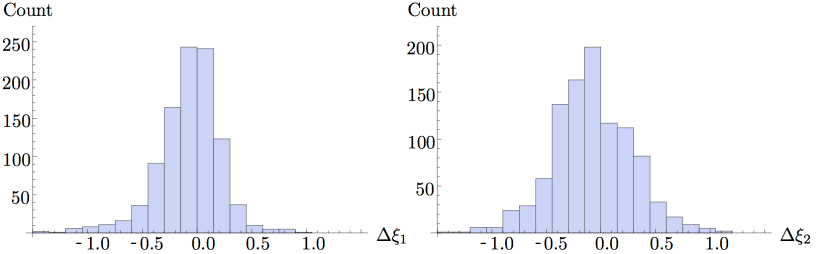
Figure 2: Example histograms of the difference $\Delta\xi_{1}=\xi_{1}^{\rm fit}-\xi_{1}^{\rm in}$ (left) and $\Delta\xi_{2}$ (right) for $\mathcal{N}_{\rm total}=100$ events in scenario a). The standard deviation of the left distribution is $\sigma_{1}=0.288$, while the mean of the individual fit errors is $\overline{\delta\xi_{1}^{\rm fit}}=0.256$. This example shows a shape that is more peaked than a normal distribution. The right distribution has $\sigma_{2}=0.362$ which is less than $\overline{\delta\xi_{1}^{\rm fit}}=0.421$, and the shape is more box-like than a normal distribution.

One may ask if the particular choices of parameter values in scenario a) have any influence on the outcome of this sensitivity study. We therefore repeat the above procedure with the following twist:

Scenario b) For each of the one thousand samples the couplings are chosen at random (32)

$$\hbox{and rescaled to abide by}\quad\xi^{\dagger}\mbox{\boldmath$A$\unboldmath}_{1}^{\rm\{full\}}\xi=1\;.$$

We generate a random set of couplings, drawn from a finite interval, which we choose symmetric around zero and universal for all couplings $\xi_{i}$, and rescale to build a sample of vectors $\vec{\xi}$. This procedure removes the preference towards particular values for the couplings, although implicitly it assumes that they are still of the same order of magnitude. Notice that, as a consequence for the condition (32), the resulting distributions in the sampled couplings $\xi_{i}$ are not flat. In Figure 3 we show the distributions for $\xi_{1}$ and $\xi_{5}$, exemplary for couplings to leptonic and radiative operators, respectively. Note that the means for the absolute values are roughly around $0.2$ in both cases, in accordance with our previous observation that couplings are of order $\mathcal{O}(0.1)$. We present the corresponding fit results in Table 3, which may be juxtaposed to the previous scenario. In general the widths $\sigma_{i}$ have increased due to the fact that one is convoluting the “fixed-coupling results” with the “coupling distributions”, leading to more pronounced shoulders in the resulting distributions. However, the mean fit uncertainties $\overline{\delta\xi^{\rm fit}_{i}}$ are roughly the same, with some entries larger than their fixed-coupling counterparts in Table 2, and some entries smaller. Our general conclusion remains unchanged.

Table 3: Histogram widths $2\sigma_{i}$ as the error estimator for samples containing $\mathcal{N}_{\rm total}$ events, as well as the mean fit uncertainty for Scenario b).

$\mathcal{N}_{\rm total}$	$(\sigma_{1},\overline{\delta\xi^{\rm fit}_{1}})$	$(\sigma_{2},\overline{\delta\xi^{\rm fit}_{2}})$	$(\sigma_{3},\overline{\delta\xi^{\rm fit}_{3}})$	$(\sigma_{4},\overline{\delta\xi^{\rm fit}_{4}})$	$(\sigma_{5},\overline{\delta\xi^{\rm fit}_{5}})$	$(\sigma_{6},\overline{\delta\xi^{\rm fit}_{6}})$
20	(0.52, 0.59)	(0.53, 0.62)	(0.57, 0.82)	(0.59, 0.82)	(0.17, 0.16)	(0.18, 0.17)
100	(0.40, 0.35)	(0.41, 0.37)	(0.45, 0.43)	(0.48, 0.43)	(0.12, 0.08)	(0.14, 0.09)
1000	(0.22, 0.18)	(0.23, 0.18)	(0.24, 0.18)	(0.22, 0.18)	(0.06, 0.04)	(0.06, 0.04)
10000	(0.09, 0.07)	(0.11, 0.07)	(0.09, 0.07)	(0.10, 0.07)	(0.02, 0.01)	(0.02, 0.01)

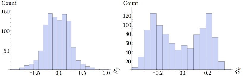
Figure 3: Distributions of randomly chosen couplings, rescaled for $\xi^{\dagger}\mbox{\boldmath$A$\unboldmath}_{1}^{\rm\{full\}}\xi=1$, i.e. Scenario b). Shown here are $\xi_{1}^{\rm in}$ (left) and $\xi_{5}^{\rm in}$ (right). The remaining couplings of leptonic operators, $\xi_{2}^{\rm in}$ through $\xi_{4}^{\rm in}$, are distributed similar to $\xi_{1}^{\rm in}$, and the second radiative coupling, $\xi_{6}^{\rm in}$, similar to $\xi_{5}^{\rm in}$. The mean absolute values of any coupling is around $0.2$.

We stress again that even with these randomized couplings for each virtual experiment there is still a build-in assumption: that all couplings are of the same order of magnitude with a flat distribution. However, depending on the explicit New Physics model (see e.g. [17, 18, 19, 20, 21, 22]) the relative importance of radiative and 4-lepton operators can be quite different. We therefore also considered a scenario in which the radiative operators may be loop induced and are therefore accompanied by Wilson coefficients that could be much smaller compared to those of the leptonic operators. We may name this Scenario b’). To be concrete, here we assume a flat distribution for the couplings of the radiative operators that have a smaller support interval, by a factor of $1/(4\pi)^{2}$. Again the absolute errors quoted in Table 3 remain the same, up to small variations. However, the corresponding distributions in the spirit of Figure 3 are such that $\overline{\xi_{1}^{\rm in}}$ is of $\mathcal{O}(1)$ – representativ for all couplings to leptonic operators – and the ones to radiative operators are of $\mathcal{O}(1/100)$. In this case it is the leptonic couplings that can be determined with a few dozen events, while the radiative ones are elusive. If this pattern were to be observed, we could also expect a suppression of the $\tau\to\ell\gamma$ decay channel. Ultimately a global fit with all relevant decay channels would be in order.

Using Asymmetries to distinguish two Scenarios.

In this subsection of the analysis the goal is to analyze the discriminating power of our approach to distinguish two different benchmark scenarios that may reflect the dynamical effects of some classes of NP models. Let us say that the dimension-6 operators (4) are induced by parity-violating interactions, i.e. one that couples only to left-handed taus or only to right-handed taus,

Scenario c) Only left-handed taus participate (33)

$$\xi=\omega\,(1,0,1,0,0,1)\qquad,\qquad\xi^{\dagger}\mbox{\boldmath$A$\unboldmath}_{1}^{\rm\{full\}}\xi=1\;,$$

Scenario d) Only right-handed taus participate (34)

$$\xi=\omega\,(0,1,0,1,1,0)\qquad,\qquad\xi^{\dagger}\mbox{\boldmath$A$\unboldmath}_{1}^{\rm\{full\}}\xi=1\;.$$

Specifically and for simplicity we consider in scenario c) equal coupling constants to all operators involving left-handed taus, while all other couplings vanish. Scenario d) is the equivalent setup with right-handed taus.

Table 4: Central values and standard deviations for the asymmetry $\mathcal{A}_{\beta}$ in both scenario c) and d), using 1000 virtual experiments.

$\mathcal{N}_{\rm total}$	$\mathcal{A}_{\beta}$(Scen. c)	$\mathcal{A}_{\beta}$(Scen. d)	Degree of Separation
5	$0.20\pm 0.44$	$-0.21\pm 0.45$	$0.36$
10	$0.19\pm 0.30$	$-0.20\pm 0.32$	$0.47$
20	$0.21\pm 0.22$	$-0.21\pm 0.21$	$0.67$
50	$0.20\pm 0.14$	$-0.20\pm 0.14$	$0.85$
100	$0.20\pm 0.10$	$-0.20\pm 0.10$	$0.95$

There are several asymmetries one can construct from the angles $\alpha,\beta,\phi_{12},\phi_{23}$. Some of them have to be combined, for example the asymmetry in $\cos\alpha$: according to Table 1 it is proportional to $\mbox{\boldmath$A$\unboldmath}_{3}^{\rm(R)}$, but for the full phase space $\mbox{\boldmath$A$\unboldmath}_{3}^{\rm\{full\}}=0$, so one needs to further cut on the full phase space to gain information. Let us instead look at the asymmetry of the angle $\beta$, to wit

$$\mathcal{A}_{\beta}=\frac{\Gamma(\cos\beta>0)-\Gamma(\cos\beta<0)}{\Gamma(\cos\beta>0)+\Gamma(\cos\beta<0)}=\frac{1}{\mathcal{N}_{\rm total}}\sum\limits_{a,c}(\mathcal{N}_{a1}^{c}-\mathcal{N}_{a2}^{c})\;.$$ (35)

Given the above two models we can readily calculate the theoretical expectations of $\mathcal{A}_{\beta}=0.202$ (Scenario c) and $\mathcal{A}_{\beta}=-0.202$ (Scenario d). Even with very few total events one can indeed already obtain an impression which scenario to prefer, as is shown in Table 4. Here, again, we have repeated the virtual experiment 1000 times to produce a distribution of results from which we estimate the typical error as the standard deviation of the distribution. The central values of the distributions fluctuate a little around the theoretical expectations due to the finite number of virtual experiments, but even with a rather small $\mathcal{N}_{\rm total}$ the likelihood for one scenario over the other is significant. The “Degree of Separation” between the two scenarios is calculated from the overlap of two normal distributions, $\rho_{c}(\mathcal{A})$ and $\rho_{c}(\mathcal{A})$, with the given central values and standard deviations of scenario c) and d), respectively,

$$\hbox{Degree of Separation}=1-\int\limits_{-\infty}^{\infty}d\mathcal{A}\,\hbox{Min}\left[\rho_{c}(\mathcal{A}),\rho_{d}(\mathcal{A})\right]\;.$$ (36)

With this definition the Degree of Separation is zero for completely overlapping distributions and asymptotically approaching 1.0 for distributions that are far apart.

4.2 Electronic final state

Table 5: Histogram widths $2\sigma_{i}$ as the error estimator for samples containing $\mathcal{N}_{\rm total}$ events, as well as the mean fit uncertainty for Scenario a).

$\mathcal{N}_{\rm total}$	$(\sigma_{1},\overline{\delta\xi^{\rm fit}_{1}})$	$(\sigma_{2},\overline{\delta\xi^{\rm fit}_{2}})$	$(\sigma_{3},\overline{\delta\xi^{\rm fit}_{3}})$	$(\sigma_{4},\overline{\delta\xi^{\rm fit}_{4}})$	$(\sigma_{5},\overline{\delta\xi^{\rm fit}_{5}})$	$(\sigma_{6},\overline{\delta\xi^{\rm fit}_{6}})$
20	(0.33, 0.42)	(0.42, 0.57)	(0.31, 0.74)	(0.31, 0.86)	(0.055, 0.039)	(0.055, 0.067)
100	(0.24, 0.27)	(0.24, 0.37)	(0.14, 0.38)	(0.18, 0.42)	(0.014, 0.014)	(0.043, 0.037)
1000	(0.12, 0.12)	(0.14, 0.16)	(0.08, 0.17)	(0.11, 0.15)	(0.004, 0.004)	(0.009, 0.010)
10000	(0.05, 0.05)	(0.10, 0.08)	(0.09, 0.09)	(0.08, 0.07)	(0.002, 0.002)	(0.004, 0.004)

Table 6: Histogram widths $2\sigma_{i}$ as the error estimator for samples containing $\mathcal{N}_{\rm total}$ events, as well as the mean fit uncertainty for Scenario b).

$\mathcal{N}_{\rm total}$	$(\sigma_{1},\overline{\delta\xi^{\rm fit}_{1}})$	$(\sigma_{2},\overline{\delta\xi^{\rm fit}_{2}})$	$(\sigma_{3},\overline{\delta\xi^{\rm fit}_{3}})$	$(\sigma_{4},\overline{\delta\xi^{\rm fit}_{4}})$	$(\sigma_{5},\overline{\delta\xi^{\rm fit}_{5}})$	$(\sigma_{6},\overline{\delta\xi^{\rm fit}_{6}})$
20	(0.38, 0.48)	(0.40, 0.49)	(0.38, 0.75)	(0.37, 0.76)	(0.060, 0.049)	(0.066, 0.052)
100	(0.28, 0.31)	(0.29, 0.34)	(0.25, 0.38)	(0.25, 0.39)	(0.037, 0.023)	(0.043, 0.026)
1000	(0.18, 0.17)	(0.18, 0.17)	(0.16, 0.15)	(0.17, 0.16)	(0.010, 0.009)	(0.010, 0.09)
10000	(0.09, 0.07)	(0.09, 0.07)	(0.08, 0.06)	(0.07, 0.06)	(0.006, 0.004)	(0.005, 0.004)

When the final-state leptons are electrons the operators and Wilson coefficients are different and in general independent from the above-mentioned decay into muons. Since electrons are much lighter than muons the entries of the $\mbox{\boldmath$A$\unboldmath}_{i}^{\rm(R)}$ matrices change, and the results can be found in Appendix C. Again we start our phenomenological game analogous to the muonic case above with

Scenario a) $$\xi^{T}=\omega\,(1.3,0.4,-4.0,0.0,2.4,1.2)$$ (37)

$$\xi^{\dagger}\mbox{\boldmath$A$\unboldmath}_{1}^{\rm\{full\}}\xi=1\qquad\Rightarrow\qquad\omega=0.0503\;.$$

Although we assume here the same relative coupling strengths as in the muonic example above, we remind the reader that there is no relation to the muonic case, and the goal is simply to gain insights into our overall ability to determine the couplings from $\mathcal{N}_{\rm total}$ events. However, the normalization condition leads to typical coupling magnitudes that are about half as large as in the muonic case, see (31). Comparing the results in Table 6 with those in Table 2, we observe that the errors on the couplings of leptonic operators are somewhat smaller for electronic final states, but not by half as is the case for the couplings themselves. However, the radiative couplings are now far easier to accurately determine. For example, with only $\mathcal{N}_{\rm total}=20$ events the typical fit result yields $\xi_{5}=0.121\pm 0.039$, whereas $\xi_{1}=0.065\pm 0.42$ does not allow us much insight.

Scenario b) For each of the one thousand samples the couplings are chosen at random (38)

$$\hbox{and rescaled to abide by}\quad\xi^{\dagger}\mbox{\boldmath$A$\unboldmath}_{1}^{\rm\{full\}}\xi=1\;.$$

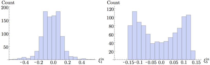
Figure 4: Distributions of randomly chosen couplings, rescaled for $\xi^{\dagger}\mbox{\boldmath$A$\unboldmath}_{1}^{\rm\{full\}}\xi=1$, i.e. Scenario b). Shown here are $\xi_{1}^{\rm in}$ (left) and $\xi_{5}^{\rm in}$ (right). The remaining couplings of leptonic operators, $\xi_{2}^{\rm in}$ through $\xi_{4}^{\rm in}$, are distributed similar to $\xi_{1}^{\rm in}$, and the second radiative coupling, $\xi_{6}^{\rm in}$, similar to $\xi_{5}^{\rm in}$. The mean absolute values of any coupling is around $0.1$.

In Figure 4 we show the distribution obtained from randomizing the couplings and rescaling. Again the typical size of couplings is of order $\mathcal{O}(0.1)$. Just as in the previous case we observe no significant difference from our finding with fixed couplings (compare Table 6 to Table 6). Next, we look at the ability to distinguish two scenarios,

Scenario c) Only left-handed taus participate (39)

$$\xi=\omega\,(1,0,1,0,0,1)\qquad,\qquad\xi^{\dagger}\mbox{\boldmath$A$\unboldmath}_{1}^{\rm\{full\}}\xi=1\;,$$

Scenario d) Only right-handed taus participate (40)

$$\xi=\omega\,(0,1,0,1,1,0)\qquad,\qquad\xi^{\dagger}\mbox{\boldmath$A$\unboldmath}_{1}^{\rm\{full\}}\xi=1\;.$$

Table 7: Central values and standard deviations for the asymmetry $\mathcal{A}_{\beta}$ in both scenario c) and d), using 1000 virtual experiments.

$\mathcal{N}_{\rm total}$	$\mathcal{A}_{\beta}$(Scen. c)	$\mathcal{A}_{\beta}$(Scen. d)	Degree of Separation
5	$0.40\pm 0.413$	$-0.39\pm 0.412$	$0.662$
10	$0.40\pm 0.280$	$-0.37\pm 0.298$	$0.817$
20	$0.39\pm 0.214$	$-0.39\pm 0.204$	$0.938$
50	$0.39\pm 0.131$	$-0.38\pm 0.129$	$0.997$
100	$0.39\pm 0.091$	$-0.39\pm 0.095$	$1.000$

The central values for the asymmetry (35) in these two scenarios is $\mathcal{A}_{\beta}=\pm 0.387$. We show the outcome of 1000 simulations for each $\mathcal{N}_{\rm total}$ in Table 7. It is notable that even very few events suffice for the distinction of these two scenarios.

5 Summary

Since the decay $\tau\to 3\ell$ is very clean, already a single event of this type would immediately imply New Physics, since the prediction of the Standard Model (extended by including the neutrino masses through the Weinberg operator) is practically zero. However, once such a decay would be observed, the nature of the underlying interaction has to be uncovered. In general this would require to study decay distributions, which is impossible with only a few events.

In this paper we have studied the LFV decays of tau leptons into three muons or electrons, including a polarization of the tau lepton. Such a polarization can be generated from running an $e^{+}e^{-}$ collider in the vicinity of the $\tau^{+}\tau^{-}$ threshold with polarized electrons and/or positrons. Experimentally this could be realized at BES III, once a polarization of the beams would become possible.

We have considered a general, model-independent set-up for the interaction mediating the $\tau$ decay, which amounts to parameterizing the effective interaction in terms of a few operators. Any specific model would correspond to specific values for the coupling constants in front of theses operators, and hence even a rough measurement of these couplings could discriminate between different NP models.

However, when determining the couplings in view of very sparse data samples we are required to define proper observables, which we have discussed in this paper. All observables are of the same nature as a forward-backward asymmetry, and therefore can be measured by a simple counting experiment.

On this basis we have performed a feasibility study on how precisely one could assess the values of individual LFV couplings, based on only a small number of total signal events. It turns out that for some simplified cases (i.e. assuming short-distance coefficients to be real, or particular chiral patterns) different NP scenarios could already be distinguished with a quite small number of events. In the case that LFV could be experimentally established, our procedure could be easily extended by refining the binning for the energy phase space and by including independent information on radiative $\tau\to\ell\gamma$ decays.

Acknowledgments

RB, TF, BOL and TM acknowledge support by the Deutsche Forschungsgemeinschaft (DFG) within the Research Unit FOR 1873 (Quark Flavour Physics and Effective Field Theories). We are also grateful to Sven Faller who collaborated with us in the early stages of this work. We further thank Danny van Dyk for helpful discussions. The research of ST was supported by the ERC Advanced Grant EFT4LHC of the European Research Council and the Cluster of Excellence Precision Physics, Fundamental Interactions and Structure of Matter (PRISMA-EXC 1098). ST is deeply grateful for extensive discussions with Florian Bernlochner.

Appendix

Appendix A Operator matrix elements

Below we list contributions to the squared amplitude $|\mathcal{M}^{\uparrow}|^{2}$. For legibility the symbol $\uparrow$ denoting that the tau lepton in polarized spin-up in the $\vec{s}$ direction is suppressed. We start with the contributions from squared leptonic operators, which are

$$|\mathcal{M}_{\rm lept}^{(LL)(LL)}|^{2} = \left|\langle\mu^{-}(p_{1})\mu^{-}(p_{2})\mu^{+}(p_{3})|H^{(LL)(LL)}_{\rm eff}|\tau^{-}(p_{\tau})\rangle\right|^{2}$$

$$= \left|\xi_{1}\right|^{2}32(p_{1}\cdot p_{2})\left[(p_{\tau}\cdot p_{3})-m_{\tau}(s\cdot p_{3})\right]\;,$$

$$|\mathcal{M}_{\rm lept}^{(RR)(RR)}|^{2} = \left|\xi_{2}\right|^{2}32(p_{1}\cdot p_{2})\left[(p_{\tau}\cdot p_{3})+m_{\tau}(s\cdot p_{3})\right]\;,$$

$$|\mathcal{M}_{\rm lept}^{(LL)(RR)}|^{2} = \left|\xi_{3}\right|^{2}8\Big{\{}(p_{1}\cdot p_{3})\left[(p_{\tau}\cdot p_{2})-m_{\tau}(s\cdot p_{2})\right]+(p_{2}\cdot p_{3})\left[(p_{\tau}\cdot p_{1})-m_{\tau}(s\cdot p_{1})\right]\Big{.}$$

$$\Big{.}\quad-m^{2}\left[(p_{\tau}\cdot p_{3})-m_{\tau}(s\cdot p_{3})\right]\Big{\}}\;,$$

$$|\mathcal{M}_{\rm lept}^{(RR)(LL)}|^{2} = \left|\xi_{4}\right|^{2}8\Big{\{}(p_{1}\cdot p_{3})\left[(p_{\tau}\cdot p_{2})+m_{\tau}(s\cdot p_{2})\right]+(p_{2}\cdot p_{3})\left[(p_{\tau}\cdot p_{1})+m_{\tau}(s\cdot p_{1})\right]\Big{.}$$ (41)

$$\Big{.}\quad-m^{2}\left[(p_{\tau}\cdot p_{3})+m_{\tau}(s\cdot p_{3})\right]\Big{\}}\;.$$

Next, the interference terms from leptonic operators, which are

$$\mathcal{M}_{\rm lept}^{(LL)(LL)}{\mathcal{M}_{\rm lept}^{(RR)(RR)}}^{*} = \xi_{1}\xi_{2}^{*}\,(-32)m_{\tau}m^{3}\;,$$

$$\mathcal{M}_{\rm lept}^{(LL)(LL)}{\mathcal{M}_{\rm lept}^{(LL)(RR)}}^{*} = \xi_{1}\xi_{3}^{*}\,8m^{2}\left[m_{\tau}(s\cdot p_{3})-(p_{\tau}\cdot p_{3})+m_{\tau}^{2}\right]\;,$$

$$\mathcal{M}_{\rm lept}^{(LL)(LL)}{\mathcal{M}_{\rm lept}^{(RR)(LL)}}^{*} = \xi_{1}\xi_{4}^{*}\,8m_{\tau}m\left[m_{\tau}(s\cdot p_{3})-(p_{\tau}\cdot p_{3})+m^{2}\right]\;,$$

$$\mathcal{M}_{\rm lept}^{(RR)(RR)}{\mathcal{M}_{\rm lept}^{(LL)(RR)}}^{*} = \xi_{2}\xi_{3}^{*}\,8m_{\tau}m\left[-m_{\tau}(s\cdot p_{3})-(p_{\tau}\cdot p_{3})+m^{2}\right]\;,$$

$$\mathcal{M}_{\rm lept}^{(RR)(RR)}{\mathcal{M}_{\rm lept}^{(RR)(LL)}}^{*} = \xi_{2}\xi_{4}^{*}\,8m^{2}\left[-m_{\tau}(s\cdot p_{3})-(p_{\tau}\cdot p_{3})+m_{\tau}^{2}\right]\;,$$

$$\mathcal{M}_{\rm lept}^{(LL)(RR)}{\mathcal{M}_{\rm lept}^{(RR)(LL)}}^{*} = \xi_{3}\xi_{4}^{*}\,8m_{\tau}m\left[(p_{1}\cdot p_{2})-2m^{2}\right]\;,$$ (42)

as well as the complex conjugate expressions. The contributions from radiative operators read

$$|\mathcal{M}_{\rm rad}^{(LR)}|^{2} = \left|\xi_{5}\right|^{2}2m_{\tau}^{2}\Big{\{}-6m^{2}$$

$$+\frac{2m^{2}}{s_{13}^{2}}(m_{\tau}^{2}-m^{2})\left(m_{\tau}^{2}-2m_{\tau}(s\cdot p_{2})-m^{2}\right)$$

$$+\frac{2m^{2}}{s_{23}^{2}}(m_{\tau}^{2}-m^{2})\left(m_{\tau}^{2}-2m_{\tau}(s\cdot p_{1})-m^{2}\right)$$

$$+\frac{2}{s_{13}s_{23}}(m_{\tau}^{4}-3m_{\tau}^{2}m^{2}+2m^{4})\left(m^{2}+m_{\tau}(s\cdot p_{1})+m_{\tau}(s\cdot p_{2})\right)$$

$$+\frac{1}{s_{13}}\Big{[}\Big{.}m_{\tau}^{4}+3m^{4}-2(m_{\tau}^{2}+3m^{2})s_{23}+2s_{23}^{2}$$

$$\qquad\quad+4m_{\tau}(2m^{2}-s_{23})(s\cdot p_{1})+2m_{\tau}(3m^{2}-2m_{\tau}^{2})(s\cdot p_{2})\Big{.}\Big{]}$$

$$+\frac{1}{s_{23}}\Big{[}\Big{.}m_{\tau}^{4}+3m^{4}-2(m_{\tau}^{2}+3m^{2})s_{13}+2s_{13}^{2}$$

$$\qquad\quad+4m_{\tau}(2m^{2}-s_{13})(s\cdot p_{2})+2m_{\tau}(3m^{2}-2m_{\tau}^{2})(s\cdot p_{1})\Big{.}\Big{]}\Big{.}\Big{\}}\;,$$

$$|\mathcal{M}_{\rm rad}^{(RL)}|^{2} = \left|\xi_{6}\right|^{2}2m_{\tau}^{2}\Big{\{}-6m^{2}$$

$$+\frac{2m^{2}}{s_{13}^{2}}(m_{\tau}^{2}-m^{2})\left(m_{\tau}^{2}+2m_{\tau}(s\cdot p_{2})-m^{2}\right)$$

$$+\frac{2m^{2}}{s_{23}^{2}}(m_{\tau}^{2}-m^{2})\left(m_{\tau}^{2}+2m_{\tau}(s\cdot p_{1})-m^{2}\right)$$

$$+\frac{2}{s_{13}s_{23}}(m_{\tau}^{4}-3m_{\tau}^{2}m^{2}+2m^{4})\left(m^{2}-m_{\tau}(s\cdot p_{1})-m_{\tau}(s\cdot p_{2})\right)$$

$$+\frac{1}{s_{13}}\Big{[}\Big{.}m_{\tau}^{4}+3m^{4}-2(m_{\tau}^{2}+3m^{2})s_{23}+2s_{23}^{2}$$

$$\qquad\quad-4m_{\tau}(2m^{2}-s_{23})(s\cdot p_{1})-2m_{\tau}(3m^{2}-2m_{\tau}^{2})(s\cdot p_{2})\Big{.}\Big{]}$$

$$+\frac{1}{s_{23}}\Big{[}\Big{.}m_{\tau}^{4}+3m^{4}-2(m_{\tau}^{2}+3m^{2})s_{13}+2s_{13}^{2}$$

$$\qquad\quad-4m_{\tau}(2m^{2}-s_{13})(s\cdot p_{2})-2m_{\tau}(3m^{2}-2m_{\tau}^{2})(s\cdot p_{1})\Big{.}\Big{]}\Big{.}\Big{\}}\;,$$

$$\mathcal{M}_{\rm rad}^{(LR)}{\mathcal{M}_{\rm rad}^{(RL)}}^{*} = \xi_{5}\xi_{6}^{*}\,(-4m_{\tau}^{3}m)\left\{4+2m^{2}\left(\frac{1}{s_{13}}+\frac{1}{s_{23}}\right)-\frac{m^{2}(m_{\tau}^{2}-m^{2})}{s_{13}s_{23}}\right\}\;.$$ (43)

The mixed leptonic radiative contributions are the only ones that contribute to $J_{4}$. We use the convention

$$\hbox{tr}\left[\gamma^{\mu}\gamma^{\nu}\gamma^{\rho}\gamma^{\sigma}\gamma_{5}\right]=-4i\varepsilon^{\mu\nu\rho\sigma}\;.$$ (44)

Since this trace is purely imaginary, we will pick up a dependence on ${\rm Im}(\xi_{i}\xi_{j}^{*})$. We find

$$\mathcal{M}_{\rm rad}^{(LR)}{\mathcal{M}_{\rm lept}^{(LL)(LL)}}^{*} = \xi_{5}\xi_{1}^{*}\,4m_{\tau}\Big{\{}\Big{.}2m_{\tau}\left(m_{\tau}^{2}-s_{13}-s_{23}\right)$$ (45)

$$+m_{\tau}m^{2}(m_{\tau}^{2}-m^{2})\left(\frac{1}{s_{13}}+\frac{1}{s_{23}}\right)$$

$$+2(m_{\tau}^{2}+m^{2}-s_{13}-s_{23})\left(\frac{1}{s_{13}}-\frac{1}{s_{23}}\right)i(\varepsilon_{\alpha\beta\gamma\delta}p_{2}^{\alpha}p_{3}^{\beta}p_{\tau}^{\gamma}s^{\delta})$$

$$+(m_{\tau}^{2}-m^{2})(m_{\tau}^{2}+m^{2}-s_{23})\frac{(s\cdot p_{1})}{s_{13}}$$

$$+(m_{\tau}^{2}-m^{2})(m_{\tau}^{2}+m^{2}-s_{13})\frac{(s\cdot p_{2})}{s_{23}}$$

$$+\left[(m_{\tau}^{2}-s_{13})^{2}-2m^{2}s_{13}+m^{4}\right]\frac{(s\cdot p_{1})}{s_{23}}$$

$$+\left[(m_{\tau}^{2}-s_{23})^{2}-2m^{2}s_{23}+m^{4}\right]\frac{(s\cdot p_{2})}{s_{13}}$$

$$-\left(m_{\tau}^{2}+s_{23}-m^{2}\right)(s\cdot p_{1})-\left(m_{\tau}^{2}+s_{13}-m^{2}\right)(s\cdot p_{2})\Big{.}\Big{\}}\;.$$

Next,

$$\mathcal{M}_{\rm rad}^{(LR)}{\mathcal{M}_{\rm lept}^{(RR)(RR)}}^{*} = \xi_{5}\xi_{2}^{*}\,4m_{\tau}m\Big{\{}\Big{.}2\left(m^{2}-s_{13}-s_{23}\right)+4m_{\tau}\left[(s\cdot p_{1})+(s\cdot p_{2})\right]$$ (46)

$$+\frac{m^{2}}{s_{13}}\left[m^{2}-m_{\tau}^{2}+2m_{\tau}(s\cdot p_{2})\right]+\frac{m^{2}}{s_{23}}\left[m^{2}-m_{\tau}^{2}+2m_{\tau}(s\cdot p_{1})\right]\Big{.}\Big{\}}\;.$$

Next,

$$\mathcal{M}_{\rm rad}^{(LR)}{\mathcal{M}_{\rm lept}^{(LL)(RR)}}^{*} = \xi_{5}\xi_{3}^{*}2m_{\tau}\Big{\{}\Big{.}m_{\tau}\left(s_{13}+s_{23}-6m^{2}\right)$$ (47)

$$+m_{\tau}m^{2}(m_{\tau}^{2}-m^{2})\left(\frac{1}{s_{13}}+\frac{1}{s_{23}}\right)$$

$$-2\left(\frac{s_{23}}{s_{13}}-\frac{s_{13}}{s_{23}}\right)i(\varepsilon_{\alpha\beta\gamma\delta}p_{2}^{\alpha}p_{3}^{\beta}p_{\tau}^{\gamma}s^{\delta})$$

$$-(m_{\tau}^{2}-m^{2})\frac{s_{23}}{s_{13}}(s\cdot p_{1})-(m_{\tau}^{2}-m^{2})\frac{s_{13}}{s_{23}}(s\cdot p_{2})$$

$$-s_{23}(s\cdot p_{1})-s_{13}(s\cdot p_{2})$$

$$-\left[(m_{\tau}^{2}-s_{13})s_{13}+m^{2}(2m_{\tau}^{2}+s_{13})\right]\frac{(s\cdot p_{1})}{s_{23}}$$

$$-\left[(m_{\tau}^{2}-s_{23})s_{23}+m^{2}(2m_{\tau}^{2}+s_{23})\right]\frac{(s\cdot p_{2})}{s_{13}}\Big{.}\Big{\}}.$$

Next,

$$\mathcal{M}_{\rm rad}^{(LR)}{\mathcal{M}_{\rm lept}^{(RR)(LL)}}^{*} = \xi_{5}\xi_{4}^{*}4m_{\tau}m\Big{\{}\Big{.}m^{2}-s_{13}-s_{23}$$ (48)

$$-\frac{m^{2}}{2}(m_{\tau}^{2}-m^{2})\left(\frac{1}{s_{13}}+\frac{1}{s_{23}}\right)$$

$$-2m_{\tau}\left(\frac{1}{s_{13}}-\frac{1}{s_{23}}\right)i(\varepsilon_{\alpha\beta\gamma\delta}p_{2}^{\alpha}p_{3}^{\beta}p_{\tau}^{\gamma}s^{\delta})$$

$$-m_{\tau}(m_{\tau}^{2}-m^{2})\frac{(s\cdot p_{1})}{s_{13}}-m_{\tau}(m_{\tau}^{2}-m^{2})\frac{(s\cdot p_{2})}{s_{23}}$$

$$-m_{\tau}(m_{\tau}^{2}-s_{13})\frac{(s\cdot p_{1})}{s_{23}}-m_{\tau}(m_{\tau}^{2}-s_{23})\frac{(s\cdot p_{2})}{s_{13}}$$

$$+m_{\tau}\left[(s\cdot p_{1})+(s\cdot p_{2})\right]\Big{.}\Big{\}}\;.$$

Now we mix the second radiative operator into the leptonic ones. The expressions are the same as we found before, except for the signs in front of the spin-vector products $(s\cdot p_{1})$ and $(s\cdot p_{2})$.

$$\mathcal{M}_{\rm rad}^{(RL)}{\mathcal{M}_{\rm lept}^{(LL)(LL)}}^{*} = \xi_{6}\xi_{1}^{*}4m_{\tau}m\Big{\{}\Big{.}2\left(m^{2}-s_{13}-s_{23}\right)-4m_{\tau}\left[(s\cdot p_{1})+(s\cdot p_{2})\right]$$ (49)

$$+\frac{m^{2}}{s_{13}}\left[m^{2}-m_{\tau}^{2}-2m_{\tau}(s\cdot p_{2})\right]+\frac{m^{2}}{s_{23}}\left[m^{2}-m_{\tau}^{2}-2m_{\tau}(s\cdot p_{1})\right]\Big{.}\Big{\}}\;.$$

Next,

$$\mathcal{M}_{\rm rad}^{(RL)}{\mathcal{M}_{\rm lept}^{(RR)(RR)}}^{*} = \xi_{6}\xi_{2}^{*}4m_{\tau}\Big{\{}\Big{.}2m_{\tau}\left(m_{\tau}^{2}-s_{13}-s_{23}\right)$$ (50)

$$+m_{\tau}m^{2}(m_{\tau}^{2}-m^{2})\left(\frac{1}{s_{13}}+\frac{1}{s_{23}}\right)$$

$$+2(m_{\tau}^{2}+m^{2}-s_{13}-s_{23})\left(\frac{1}{s_{13}}-\frac{1}{s_{23}}\right)i(\varepsilon_{\alpha\beta\gamma\delta}p_{2}^{\alpha}p_{3}^{\beta}p_{\tau}^{\gamma}s^{\delta})$$

$$-(m_{\tau}^{2}-m^{2})(m_{\tau}^{2}+m^{2}-s_{23})\frac{(s\cdot p_{1})}{s_{13}}$$

$$-(m_{\tau}^{2}-m^{2})(m_{\tau}^{2}+m^{2}-s_{13})\frac{(s\cdot p_{2})}{s_{23}}$$

$$-\left[(m_{\tau}^{2}-s_{13})^{2}-2m^{2}s_{13}+m^{4}\right]\frac{(s\cdot p_{1})}{s_{23}}$$

$$-\left[(m_{\tau}^{2}-s_{23})^{2}-2m^{2}s_{23}+m^{4}\right]\frac{(s\cdot p_{2})}{s_{13}}$$

$$+\left(m_{\tau}^{2}+s_{23}-m^{2}\right)(s\cdot p_{1})+\left(m_{\tau}^{2}+s_{13}-m^{2}\right)(s\cdot p_{2})\Big{.}\Big{\}}\;.$$

Next,

$$\mathcal{M}_{\rm rad}^{(RL)}{\mathcal{M}_{\rm lept}^{(LL)(RR)}}^{*} = \xi_{6}\xi_{3}^{*}4m_{\tau}m\Big{\{}\Big{.}m^{2}-s_{13}-s_{23}$$ (51)

$$-\frac{m^{2}}{2}(m_{\tau}^{2}-m^{2})\left(\frac{1}{s_{13}}+\frac{1}{s_{23}}\right)$$

$$-2m_{\tau}\left(\frac{1}{s_{13}}-\frac{1}{s_{23}}\right)i(\varepsilon_{\alpha\beta\gamma\delta}p_{2}^{\alpha}p_{3}^{\beta}p_{\tau}^{\gamma}s^{\delta})$$

$$+m_{\tau}(m_{\tau}^{2}-m^{2})\frac{(s\cdot p_{1})}{s_{13}}+m_{\tau}(m_{\tau}^{2}-m^{2})\frac{(s\cdot p_{2})}{s_{23}}$$

$$+m_{\tau}(m_{\tau}^{2}-s_{13})\frac{(s\cdot p_{1})}{s_{23}}+m_{\tau}(m_{\tau}^{2}-s_{23})\frac{(s\cdot p_{2})}{s_{13}}$$

$$-m_{\tau}\left[(s\cdot p_{1})+(s\cdot p_{2})\right]\Big{.}\Big{\}}$$

And finally

$$\mathcal{M}_{\rm rad}^{(RL)}{\mathcal{M}_{\rm lept}^{(RR)(LL)}}^{*} = \xi_{6}\xi_{4}^{*}2m_{\tau}\Big{\{}\Big{.}m_{\tau}\left(s_{13}+s_{23}-6m^{2}\right)$$ (52)

$$+m_{\tau}m^{2}(m_{\tau}^{2}-m^{2})\left(\frac{1}{s_{13}}+\frac{1}{s_{23}}\right)$$

$$-2\left(\frac{s_{23}}{s_{13}}-\frac{s_{13}}{s_{23}}\right)i(\varepsilon_{\alpha\beta\gamma\delta}p_{2}^{\alpha}p_{3}^{\beta}p_{\tau}^{\gamma}s^{\delta})$$

$$+(m_{\tau}^{2}-m^{2})\frac{s_{23}}{s_{13}}(s\cdot p_{1})+(m_{\tau}^{2}-m^{2})\frac{s_{13}}{s_{23}}(s\cdot p_{2})$$

$$+s_{23}(s\cdot p_{1})+s_{13}(s\cdot p_{2})$$

$$+\left[(m_{\tau}^{2}-s_{13})s_{13}+m^{2}(2m_{\tau}^{2}+s_{13})\right]\frac{(s\cdot p_{1})}{s_{23}}$$

$$+\left[(m_{\tau}^{2}-s_{23})s_{23}+m^{2}(2m_{\tau}^{2}+s_{23})\right]\frac{(s\cdot p_{2})}{s_{13}}\Big{.}\Big{\}}.$$

Appendix B Analytic Calculation of the Matrices $\mbox{\boldmath$A$\unboldmath}_{i}^{\rm(R)}$

In the following, we show two examples how to obtain analytic results for the matrices $A_{i}^{(R)}$ as an expansion in terms of the small parameter $\epsilon=m/m_{\tau}$, keeping terms up to $\mathcal{O}(\epsilon^{2})$.

Integrating a constant over the full phase space.

We integrate the constant $1/m_{\tau}^{2}$ over the energies $E_{2}$ and $E_{3}$. At leading power in $\epsilon$ there is no problem and the result is $1/8$. However, at subleading power divergences appear at the border of the phase space. We regulate these divergencies by manually introducing

$$\frac{1}{m_{\tau}^{2}}\longrightarrow\left(\frac{E_{2}}{\mu_{1}}\right)^{\eta_{1}}\left(\frac{s_{13}}{\mu_{2}^{2}}\right)^{\eta_{2}}\frac{1}{m_{\tau}^{2}}\;,$$ (53)

and taking the simultaneous limit $\eta_{1,2}\to 0$ in the end. The first integration – over $E_{3}$, say – is straight forward. We then distinguish three regions.

• Treating $E_{2}$ as $\mathcal{O}(m_{\tau})$ yields

  $$I_{\rm hard}=\frac{1}{8}\underbrace{-\frac{m^{2}}{2m_{\tau}^{2}\eta_{1}}-\frac{m^{2}}{2m_{\tau}^{2}\eta_{2}}}_{\rm singular}+\frac{m^{2}}{m_{\tau}^{2}}\left[\frac{3}{4}-\left(\frac{1}{2}+\frac{\eta_{1}}{2\eta_{2}}\right)\ln\frac{m_{\tau}}{2\mu_{1}}-\left(1+\frac{\eta_{2}}{\eta_{1}}\right)\ln\frac{m_{\tau}}{\mu_{2}}\right]\;.$$ (54)

• When treating $E_{2}\sim m$ one needs to integrate $E_{2}\in[m,\infty]$. This gives

  $$I_{\rm soft\;E_{2}}=\underbrace{\frac{m^{2}}{2m_{\tau}^{2}\eta_{1}}}_{\rm singular}+\frac{m^{2}}{m_{\tau}^{2}}\left[-\frac{1}{4}+\frac{1}{2}\ln\frac{m}{2\mu_{1}}+\frac{\eta_{2}}{\eta_{1}}\ln\frac{m_{\tau}}{\mu_{2}}\right]\;.$$ (55)

• $E_{2}$ is near its maximum value is akin to treating $s_{13}\sim m^{2}$ and integrating $s_{13}\in[4m^{2},\infty]$. We find

  $$I_{\rm soft\;s_{13}}=\underbrace{\frac{m^{2}}{2m_{\tau}^{2}\eta_{2}}}_{\rm singular}+\frac{m^{2}}{m_{\tau}^{2}}\left[-\frac{1}{2}+\ln\frac{m}{\mu_{2}}+\frac{\eta_{1}}{2\eta_{2}}\ln\frac{m_{\tau}}{2\mu_{1}}\right]\;.$$ (56)

The singular terms cancel in the sum of these contributions, and the dependence on the auxiliary scales $\mu_{i}$ drops out as well, resulting in

$$I_{\rm hard}+I_{\rm soft\;E_{2}}+I_{\rm soft\;s_{13}}=\frac{1}{8}+\frac{3m^{2}}{2m_{\tau}^{2}}\ln\frac{m}{m_{\tau}}.$$ (57)

Integrating singular pieces from the radiative contributions.

Much more challenging contributions arise from the radiative operators, where the intermediate photon propagator leads to integrands proportional to inverse powers of the invariants $s_{ij}$. The most singular expression in (A), for example, is

$$\frac{1}{s_{13}s_{23}}=\frac{1}{(s_{13}+s_{23})s_{13}}+\frac{1}{(s_{13}+s_{23})s_{23}}\;.$$ (58)

For definiteness we are therefore focussing here on the integral

$$S(m/m_{\tau})=\int\limits_{\rm phase\;space}dE_{2}\,dE_{3}\frac{m_{\tau}^{2}}{(s_{13}+s_{23})s_{13}}=\int\limits_{\rm phase\;space}dE_{2}\,dE_{3}\frac{m_{\tau}^{2}}{(2m_{\tau}E_{3}+2m^{2})s_{13}}\;,$$ (59)

which has a soft $E_{3}$ and a collinear $s_{13}$ singular structure. We may identify four different regions to solve this integral.

1. The soft $E_{2}$ region, where $E_{2}\sim m$ and $b_{2}$ can be resolved. This region only becomes relevant for power corrections.

2. The collinear $s_{13}\sim m^{2}$ region, where $E_{2}$ is nearly at the endpoint, namely of the order $\mathcal{O}(m^{2}/m_{\tau})$ away from its maximum. Here $d_{2}$ can be resolved.

3. The soft $E_{3}$ region, where $E_{2}$ is of order $\mathcal{O}(m)$ away from its maximum.

4. The bulk.

We aim to distinguish these regions in a single, one-dimensional integral over a variable that differentiates between the four regions in terms of its power counting. To this end we perform the first integration over $E_{3}$ without approximation and are left with a single integral over $E_{2}$. Let us now define $\tilde{E}_{2}$ as the energy variable that is smallest for maximal $E_{2}$, i.e. $E_{2}=\frac{m_{\tau}^{2}-3m^{2}}{2m_{\tau}}-\tilde{E}_{2}$. Finally we define the variable $\rho=\tilde{E}_{2}/E_{2}$, which will accomplish our goal: After substituting the $E_{2}=\frac{m_{\tau}^{2}-3m^{2}}{2m_{\tau}}\frac{1}{1+\rho}$ integration variable for $\rho\in[0,\frac{m_{\tau}}{2m}-1-\frac{3m}{2m_{\tau}}]$ we find the following in the above four regions and name them

1. $\rho\sim m_{\tau}/m$, label “uhard”,

2. $\rho\sim m^{2}/m_{\tau}^{2}$, label “usoft”,

3. $\rho\sim m/m_{\tau}$, label “soft”,

4. $\rho\sim 1$, label “hard”.

Finally we need to choose a regulator common in all regions. While $\rho^{\eta}\stackrel{{\scriptstyle\eta\to 0}}{{\longrightarrow}}1$ is quite suitable we find that the regulator

$$\left(\frac{\sqrt{s_{13}}+\sqrt{s_{13}-4m^{2}}}{\sqrt{s_{13}}-\sqrt{s_{13}-4m^{2}}}\frac{m^{2}}{\mu_{1}^{2}}\right)^{\eta}\left(\frac{E_{2}}{\mu_{2}}\right)^{2\eta}\stackrel{{\scriptstyle\eta\to 0}}{{\longrightarrow}}1$$ (60)

is more advantageous as it simplifies the practical calculation. We find

• Usoft region: Expanding the integrand and integrating $0\leq\rho<\infty$ we find

  $$S_{us}=\frac{1}{4\eta^{2}}+\frac{1}{2\eta}\left[\ln\frac{m_{\tau}m}{2\mu_{1}\mu_{2}}-\frac{2m^{2}}{m_{\tau}^{2}}\right]+\hbox{finite.}$$ (61)

• Soft region: Expanding the integrand and integrating $0\leq\rho<\infty$ we find

  $$S_{s}=-\frac{1}{2\eta^{2}}+\frac{1}{2\eta}\left[\ln\frac{4\mu_{1}^{2}\mu_{2}^{2}}{m_{\tau}^{3}m}+\frac{m^{2}}{2m_{\tau}^{2}}\right]+\hbox{finite.}$$ (62)

• Hard region: Expanding the integrand and integrating $0\leq\rho<\infty$ we find

  $$S_{h}=\frac{1}{4\eta^{2}}+\frac{1}{2\eta}\left[\ln\frac{m_{\tau}^{2}}{2\mu_{1}\mu_{2}}+\frac{m^{2}}{m_{\tau}^{2}}\right]+\hbox{finite.}$$ (63)

• Uhard region: Expanding the integrand and integrating $0\leq\rho\leq\frac{m_{\tau}}{2m}-1-\frac{3m}{2m_{\tau}}$ we find

  $$S_{uh}=\frac{1}{4\eta}\frac{m^{2}}{m_{\tau}^{2}}+\hbox{finite.}$$ (64)

Again all the double and single divergences cancel in the sum of the regions and we obtain a leading double logarithm free of any regulators, to wit

$$S(m/m_{\tau})=\left[\frac{1}{4}\ln^{2}\frac{m}{m_{\tau}}-\frac{\pi^{2}}{16}\right]+\frac{m^{2}}{m_{\tau}^{2}}\left[\frac{9}{8}-\frac{5}{4}\ln\frac{m}{m_{\tau}}\right]\;.$$ (65)

Armed with the techniques discussed above we are able to state some analytic results. We find in terms of $\epsilon=m/m_{\tau}$

$$\mbox{\boldmath$A$\unboldmath}_{1}^{\rm\{full\}}=\left(\begin{array}[]{cccccc}\mbox{\boldmath$1$\unboldmath}-24\epsilon^{2}&0&4\epsilon^{2}&-2\epsilon&\mbox{\boldmath$2$\unboldmath}-48\epsilon^{2}&-4\epsilon\\ 0&\mbox{\boldmath$1$\unboldmath}-24\epsilon^{2}&-2\epsilon&4\epsilon^{2}&-4\epsilon&\mbox{\boldmath$2$\unboldmath}-48\epsilon^{2}\\ 4\epsilon^{2}&-2\epsilon&\mbox{\boldmath$\frac{1}{2}$\unboldmath}-14\epsilon^{2}&\epsilon&\mbox{\boldmath$1$\unboldmath}-24\epsilon^{2}&-2\epsilon\\ -2\epsilon&4\epsilon^{2}&\epsilon&\mbox{\boldmath$\frac{1}{2}$\unboldmath}-14\epsilon^{2}&-2\epsilon&\mbox{\boldmath$1$\unboldmath}-24\epsilon^{2}\\ \mbox{\boldmath$2$\unboldmath}-48\epsilon^{2}&-4\epsilon&\mbox{\boldmath$1$\unboldmath}-24\epsilon^{2}&-2\epsilon&\mbox{\boldmath$a^{\rm\{full\}}_{55}$\unboldmath}&-12\epsilon\\ -4\epsilon&\mbox{\boldmath$2$\unboldmath}-48\epsilon^{2}&-2\epsilon&\mbox{\boldmath$1$\unboldmath}-24\epsilon^{2}&-12\epsilon&\mbox{\boldmath$a^{\rm\{full\}}_{66}$\unboldmath}\end{array}\right)+\mathcal{O}(\epsilon^{3})\;,$$ (66)

where

$$a^{\rm\{full\}}_{55}=a^{\rm\{full\}}_{66}=-(8\ln\epsilon+11)+\left[12\ln^{2}\epsilon+36\ln\epsilon+50-3\pi^{2}\right]\epsilon^{2}\;.$$ (67)

Appendix C Numerical Results for the Matrices $\mbox{\boldmath$A$\unboldmath}_{i}^{\rm(R)}$

For muons in the final state we use $m=105.658$ MeV and $m_{\tau}=1776.82$ MeV, which corresponds to $\epsilon=0.0595$.

$$\mbox{\boldmath$A$\unboldmath}_{1}^{\rm\{full\}} \simeq \left(\begin{array}[]{cccccc}0.919&-0.004&0.012&-0.104&1.838&-0.217\\ -0.004&0.919&-0.104&0.012&-0.217&1.838\\ 0.012&-0.104&0.453&0.050&0.919&-0.109\\ -0.104&0.012&0.050&0.453&-0.109&0.919\\ 1.838&-0.217&0.919&-0.109&11.635&-0.628\\ -0.217&1.838&-0.109&0.919&-0.628&11.635\end{array}\right)$$ (74)

$$\mbox{\boldmath$A$\unboldmath}_{2}^{\rm\{full\}} \simeq \left(\begin{array}[]{cccccc}0.889&0&-0.006&-0.103&1.461&-0.210\\ 0&-0.889&0.103&0.006&0.210&-1.461\\ -0.006&0.103&-0.159&0&-0.848&0.185\\ -0.103&0.006&0&0.159&-0.185&0.848\\ 1.461&0.210&-0.848&-0.185&-4.344&0\\ -0.210&-1.461&0.185&0.848&0&4.344\end{array}\right)$$ (81)

$$\mbox{\boldmath$A$\unboldmath}_{3}^{\rm\{full\}} = \mbox{\boldmath$A$\unboldmath}_{4}^{\rm\{full\}}=0$$ (82)

For the part of the phase space where $\cos\phi_{23}>0$ we find

$$\mbox{\boldmath$A$\unboldmath}_{1}^{\{\cos\phi_{23}>0\}} \simeq \left(\begin{array}[]{cccccc}0.245&-0.001&0.003&-0.019&0.572&-0.041\\ -0.001&0.245&-0.019&0.003&-0.041&0.572\\ 0.003&-0.019&0.081&0.015&0.175&-0.020\\ -0.019&0.003&0.015&0.081&-0.020&0.176\\ 0.572&-0.041&0.175&-0.020&4.320&-0.139\\ -0.041&0.572&-0.020&0.175&-0.139&4.320\end{array}\right)\;,$$ (89)

$$\mbox{\boldmath$A$\unboldmath}_{2}^{\{\cos\phi_{23}>0\}} \simeq \left(\begin{array}[]{cccccc}0.235&0&-0.001&-0.018&0.417&-0.038\\ 0&-0.235&0.018&0.001&0.038&-0.417\\ -0.001&0.018&0.009&0&-0.145&0.041\\ -0.018&0.001&0&-0.009&-0.041&0.145\\ 0.417&0.038&-0.145&-0.041&-1.831&0\\ -0.038&-0.417&0.041&0.145&0&1.831\end{array}\right)\;,$$ (96)

$$\mbox{\boldmath$A$\unboldmath}_{3}^{\{\cos\phi_{23}>0\}} \simeq \left(\begin{array}[]{cccccc}0&0&0&0&-0.276&-0.0005\\ 0&0&0&0&0.0005&0.276\\ 0&0&0.037&0&0.162&-0.036\\ 0&0&0&-0.037&0.036&-0.162\\ -0.276&0.0005&0.162&0.036&-1.489&0\\ -0.0005&0.276&-0.036&-0.162&0&1.489\end{array}\right)\;,$$ (103)

$$\mbox{\boldmath$A$\unboldmath}_{4}^{\{\cos\phi_{23}>0\}} \simeq \left(\begin{array}[]{cccccc}0&0&0&0&0.253i&0\\ 0&0&0&0&0&0.253i\\ 0&0&0&0&-0.162i&-0.034i\\ 0&0&0&0&-0.034i&-0.162i\\ -0.253i&0&0.162i&0.034i&0&0\\ 0&-0.253i&0.034i&0.162i&0&0\end{array}\right)\;,$$ (110)

and for R$=\{\cos\phi_{12}>0\}$ we find

$$\mbox{\boldmath$A$\unboldmath}_{1}^{\{\cos\phi_{12}>0\}} \simeq \left(\begin{array}[]{cccccc}0.083&-0.001&0.002&-0.032&0.100&-0.065\\ -0.001&0.083&-0.032&0.002&-0.065&0.100\\ 0.002&-0.032&0.121&0.002&0.272&-0.033\\ -0.032&0.002&0.002&0.121&-0.033&0.272\\ 0.100&-0.065&0.272&-0.033&1.001&-0.141\\ -0.065&0.100&-0.033&0.272&-0.141&1.001\end{array}\right)\;,$$ (117)

$$\mbox{\boldmath$A$\unboldmath}_{2}^{\{\cos\phi_{12}>0\}} \simeq \left(\begin{array}[]{cccccc}0.082&0&-0.002&-0.032&0.084&-0.064\\ 0&-0.082&0.032&0.002&0.064&-0.084\\ -0.002&0.032&-0.098&0&-0.269&0.037\\ -0.032&0.002&0&0.098&-0.037&0.269\\ 0.084&0.064&-0.269&-0.037&-0.793&0\\ -0.064&-0.084&0.037&0.269&0&0.793\end{array}\right)\;,$$ (124)

$$\mbox{\boldmath$A$\unboldmath}_{3}^{\{\cos\phi_{12}>0\}} = \mbox{\boldmath$A$\unboldmath}_{4}^{\{\cos\phi_{12}>0\}}=0\;.$$ (125)

Now we repeat the calculation for electrons in the final state. Here $m=510.9989$ KeV. This means that $\epsilon=0.0002876$ is much smaller and we can observe the structure of the matrices much easier. We find

$$\mbox{\boldmath$A$\unboldmath}_{1}^{\rm\{full\}} = \left(\begin{array}[]{cccccc}1.00&0&0&0&2.00&0\\ 0&1.00&0&0&0&2.00\\ 0&0&0.50&0&1.00&0\\ 0&0&0&0.50&0&1.00\\ 2.00&0&1.00&0&54.23&0\\ 0&2&0&1.00&0&54.23\end{array}\right)+\mathcal{O}(10^{-3})\;,$$ (132)

$$\mbox{\boldmath$A$\unboldmath}_{2}^{\rm\{full\}} = \left(\begin{array}[]{cccccc}1.00&0&0&0&2.00&0\\ 0&-1.00&0&0&0&-2.00\\ 0&0&-0.17&0&-1.00&0\\ 0&0&0&0.17&0&1.00\\ 2.00&0&-1.00&0&-42.26&0\\ 0&-2.00&0&1.00&0&42.26\end{array}\right)+\mathcal{O}(10^{-3})\;,$$ (139)

$$\mbox{\boldmath$A$\unboldmath}_{3}^{\rm\{full\}} = \mbox{\boldmath$A$\unboldmath}_{4}^{\rm\{full\}}=0\;,$$ (140)

$$\mbox{\boldmath$A$\unboldmath}_{1}^{\{\cos\phi_{23}>0\}} = \left(\begin{array}[]{cccccc}0.27&0&0&0&0.64&0\\ 0&0.27&0&0&0&0.64\\ 0&0&0.09&0&0.18&0\\ 0&0&0&0.09&0&0.18\\ 0.64&0&0.18&0&25.22&0\\ 0&0.64&0&0.18&0&25.22\\ \end{array}\right)+\mathcal{O}(10^{-3})\;,$$ (147)

$$\mbox{\boldmath$A$\unboldmath}_{2}^{\{\cos\phi_{23}>0\}} = \left(\begin{array}[]{cccccc}0.27&0&0&0&0.64&0\\ 0&-0.27&0&0&0&-0.64\\ 0&0&0.01&0&-0.18&0\\ 0&0&0&-0.01&0&0.18\\ 0.64&0&-0.18&0&-20.60&0\\ 0&-0.64&0&0.18&0&20.60\\ \end{array}\right)+\mathcal{O}(10^{-3})\;,$$ (154)

$$\mbox{\boldmath$A$\unboldmath}_{3}^{\{\cos\phi_{23}>0\}} = \left(\begin{array}[]{cccccc}0&0&0&0&-0.63&0\\ 0&0&0&0&0&0.63\\ 0&0&0.04&0&0.36&0\\ 0&0&0&-0.04&0&-0.36\\ -0.63&0&0.36&0&-4.57&0\\ 0&0.63&0&-0.36&0&4.57\\ \end{array}\right)+\mathcal{O}(10^{-3})\;,$$ (161)

$$\mbox{\boldmath$A$\unboldmath}_{4}^{\{\cos\phi_{23}>0\}} = \left(\begin{array}[]{cccccc}0&0&0&0&0.63i&0\\ 0&0&0&0&0&0.63i\\ 0&0&0&0&-0.36i&0\\ 0&0&0&0&0&-0.36i\\ -0.63i&0&0.36i&0&0&0\\ 0&-0.63i&0&0.36i&0&0\\ \end{array}\right)+\mathcal{O}(10^{-3})\;,$$ (168)

$$\mbox{\boldmath$A$\unboldmath}_{1}^{\{\cos\phi_{12}>0\}} = \left(\begin{array}[]{cccccc}0.08&0&0&0&0.09&0\\ 0&0.08&0&0&0&0.09\\ 0&0&0.14&0&0.32&0\\ 0&0&0&0.14&0&0.32\\ 0.09&0&0.32&0&1.52&0\\ 0&0.09&0&0.32&0&1.52\\ \end{array}\right)+\mathcal{O}(10^{-3})\;,$$ (175)

$$\mbox{\boldmath$A$\unboldmath}_{2}^{\{\cos\phi_{12}>0\}} = \left(\begin{array}[]{cccccc}0.08&0&0&0&0.09&0\\ 0&-0.08&0&0&0&-0.09\\ 0&0&-0.11&0&-0.32&0\\ 0&0&0&0.11&0&0.32\\ 0.09&0&-0.32&0&-1.32&0\\ 0&-0.09&0&0.32&0&1.32\\ \end{array}\right)+\mathcal{O}(10^{-3})\;,$$ (182)

$$\mbox{\boldmath$A$\unboldmath}_{3}^{\{\cos\phi_{12}>0\}} = \mbox{\boldmath$A$\unboldmath}_{4}^{\{\cos\phi_{12}>0\}}=0\;.$$ (183)

References

- [1] M. Raidal, A. van der Schaaf, I. Bigi, M. L. Mangano, Y. K. Semertzidis, S. Abel, S. Albino and S. Antusch et al., “Flavour physics of leptons and dipole moments,” Eur. Phys. J. C 57 (2008) 13 [arXiv:0801.1826 [hep-ph]].
- [2] R. Aaij et al. [LHCb Collaboration], “Search for the lepton flavour violating decay ,” JHEP 1502, 121 (2015) [arXiv:1409.8548 [hep-ex]].
- [3] R. Aaij et al. [LHCb Collaboration], “Test of lepton universality using decays,” Phys. Rev. Lett. 113, no. 15, 151601 (2014) [arXiv:1406.6482 [hep-ex]].
- [4] CMS Collaboration [CMS Collaboration], “Search for Lepton Flavour Violating Decays of the Higgs Boson,” CMS-PAS-HIG-14-005. Dependence,” JHEP 1310 (2013) 087 [arXiv:1308.2627 [hep-ph]].
- [5] E. E. Jenkins, A. V. Manohar and M. Trott, “Renormalization Group Evolution of the Standard Model Dimension Six Operators II: Yukawa Dependence,” JHEP 1401 (2014) 035 [arXiv:1310.4838 [hep-ph], arXiv:1310.4838].
- [6] R. Alonso, E. E. Jenkins, A. V. Manohar and M. Trott, “Renormalization Group Evolution of the Standard Model Dimension Six Operators III: Gauge Coupling Dependence and Phenomenology,” JHEP 1404 (2014) 159 [arXiv:1312.2014 [hep-ph]].
- [7] E. E. Jenkins, A. V. Manohar and M. Trott, “Renormalization Group Evolution of the Standard Model Dimension Six Operators I: Formalism and lambda
- [8] B. M. Dassinger, T. Feldmann, T. Mannel and S. Turczyk, “Model-independent analysis of lepton flavour violating tau decays,” JHEP 0710, 039 (2007) [arXiv:0707.0988 [hep-ph]].
- [9] T. Mannel, “Lepton Flavour Violating Decays with Polarization,” Nucl. Phys. Proc. Suppl. 248-250, 3 (2014).
- [10] Y. S. Tsai, “Production of polarized tau pairs and tests of CP violation using polarized colliders near threshold,” Phys. Rev. D 51 (1995) 3172 [hep-ph/9410265].
- [11] T. Goto, Y. Okada and Y. Yamamoto, “Tau and muon lepton flavor violations in the littlest Higgs model with T-parity,” Phys. Rev. D 83, 053011 (2011) [arXiv:1012.4385 [hep-ph]].
- [12] W. Buchmüller and D. Wyler, “Effective Lagrangian Analysis of New Interactions and Flavor Conservation,” Nucl. Phys. B 268 (1986) 621.
- [13] B. Grzadkowski, M. Iskrzynski, M. Misiak and J. Rosiek, “Dimension-Six Terms in the Standard Model Lagrangian,” JHEP 1010 (2010) 085 [arXiv:1008.4884 [hep-ph]].
- [14] R. Alonso, B. Grinstein and J. Martin Camalich, “ gauge invariance and the shape of new physics in rare decays,” Phys. Rev. Lett. 113 (2014) 241802 [arXiv:1407.7044 [hep-ph]].
- [15] O. Catà and M. Jung, “Signatures of a nonstandard Higgs from flavor physics,” arXiv:1505.05804 [hep-ph].
- [16] M. Beneke and V. A. Smirnov, “Asymptotic expansion of Feynman integrals near threshold,” Nucl. Phys. B 522, 321 (1998) [hep-ph/9711391]. For a review, see V. A. Smirnov, “Applied asymptotic expansions in momenta and masses,” Springer Tracts Mod. Phys. 177, 1 (2002).
- [17] J. R. Ellis, J. Hisano, M. Raidal and Y. Shimizu, “A New parametrization of the seesaw mechanism and applications in supersymmetric models,” Phys. Rev. D 66 (2002) 115013 [hep-ph/0206110].
- [18] A. Brignole and A. Rossi, “Anatomy and phenomenology of lepton flavor violation in the MSSM,” Nucl. Phys. B 701 (2004) 3 [hep-ph/0404211].
- [19] P. Paradisi, “Higgs-mediated and transitions in II Higgs doublet model and supersymmetry,” JHEP 0602 (2006) 050 [hep-ph/0508054].
-
[20]
M. Blanke, A. J. Buras, B. Duling, A. Poschenrieder and C. Tarantino,
“Charged Lepton Flavour Violation and in the Littlest Higgs Model with T-Parity: A Clear Distinction from Supersymmetry,”
JHEP 0705 (2007) 013
[hep-ph/0702136];
M. Blanke, A. J. Buras, B. Duling, S. Recksiegel and C. Tarantino, “FCNC Processes in the Littlest Higgs Model with T-Parity: a 2009 Look,” Acta Phys. Polon. B 41 (2010) 657 [arXiv:0906.5454 [hep-ph]]. - [21] A. G. Akeroyd, M. Aoki and H. Sugiyama, “Lepton Flavour Violating Decays and in the Higgs Triplet Model,” Phys. Rev. D 79 (2009) 113010 [arXiv:0904.3640 [hep-ph]].
- [22] A. J. Buras, B. Duling, T. Feldmann, T. Heidsieck and C. Promberger, “Lepton Flavour Violation in the Presence of a Fourth Generation of Quarks and Leptons,” JHEP 1009 (2010) 104 [arXiv:1006.5356 [hep-ph]].