Deep CNN Ensemble with Data Augmentation for Object Detection
Abstract
We report on the methods used in our recent DeepEnsembleCoco submission to the PASCAL VOC 2012 challenge, which achieves state-of-the-art performance on the object detection task. Our method is a variant of the R-CNN model proposed by Girshick et al. [4] with two key improvements to training and evaluation. First, our method constructs an ensemble of deep CNN models with different architectures that are complementary to each other. Second, we augment the PASCAL VOC training set with images from the Microsoft COCO dataset to significantly enlarge the amount training data. Importantly, we select a subset of the Microsoft COCO images to be consistent with the PASCAL VOC task. Results on the PASCAL VOC evaluation server show that our proposed method outperform all previous methods on the PASCAL VOC 2012 detection task at time of submission.
1 Introduction
In recent years, advances in deep learning have dramatically boosted the performance of object recognition, detection and segmentation tasks (e.g., see [6], [4] and [8], respectively). Large-scale convolutional neural networks (CNNs) pretrained on large datasets, such as ImageNet [1], have demonstrated consistent improvement and generalizability across other smaller datasets and all current state-of-the-art results on the well known PASCAL VOC dataset [2] use this approach. Thus, an emergent trend in developing CNN models for computer vision applications is to start from a pretrained neural network and then fine tune the parameters for the task at hand, such as detection, segmentation, or activity recognition, and specific domain (i.e., dataset).
In addition, current best practice suggests that combining the output from several models and augmenting training data to improve the variability of instances seen during learning are further ingredients necessary for achieving state-of-the-art performance. Both of these are well known techniques in the machine learning community and relate to model averaging and over-fitting prevention. However, precise details in their implementation can dramatically running times and effectiveness.
In this technical report we detail our procedure for achieving state-of-the-art performance on the PASCAL VOC detection task. Different from existing methods, which use a single CNN model fine tuned on the PASCAL VOC training set, we combine the practices outlined above. Specifically, we construct an ensemble of CNN models with different architectures with parameters learned on different subsets of our augmented training set—a combination of the original PASCAL VOC training set and the much larger Microsoft COCO dataset [7]. We include experimental analysis on components of our model and the final combined model that was submitted to the PASCAL VOC evaluation server and achieved state-of-the-art results at the time of submission (3 May 2015).111Our submission was subsequently beaten by the method of Gidaris and Komodakis [3] on 9 May 2015..
2 Related Work
The introduction of the R-CNN approach by Girshick et al. [4] opened the door for features obtained through deep learning to improve object detection performance on the PASCAL VOC dataset. In their work, AlexNet CNN architecture [6] was used to extract a set of deep features from arbitrary rectangular regions and used for object classification. Since the introduction of AlexNet, deep learning has advanced significantly both in terms of model architecture and training methods. We hypothesize that improving the feature extraction part of the pipeline by combining the recent advances in deep learning can boost model performance. To this end, our work replaces the single AlexNet model with an ensemble of different models, namely GoogleNet [11] and VGG-16 [10]. These two recent models pushed the error rate to below 10% on ImageNet Large Scale Visual Recognition Challenge (ILSVRC) 2014 competition [9]. In addition to the improved network architectures, we also explore augmenting the training dataset with images from the recently introduced Microsoft COCO dataset [7].
3 Deep Ensemble Approach
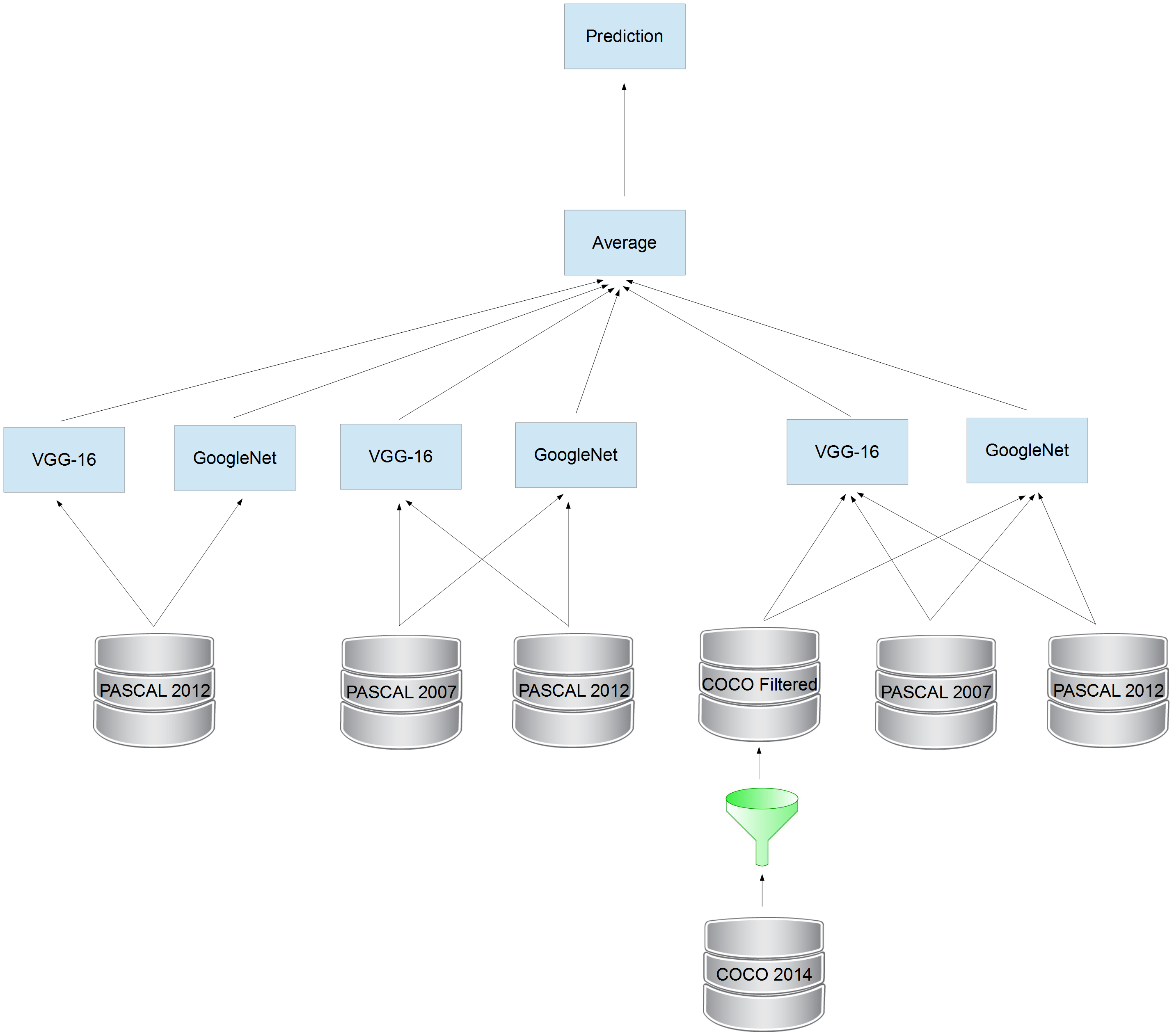
We proposed an improved variant of the Region CNN (R-CNN) method of Girshick et al. [4] for better object detection. The improvement comes from three well known but essential machine learning practices: starting from good initial parameters, averaging models, and using as much data as possible for training. An illustration of our method is shown in Figure 1 and overview as follows:
- •
-
•
We next refine the network parameters using combinations of existing datasets in three different ways. First, using the PASCAL VOC 2012 train set [2]. Second, using a merged training set consisting of all images from PASCAL VOC 2007 trainval and PASCAL VOC 2012 train. And third, using the above augmented with Microsoft COCO 2014 trainval [7]. In the following we refer to these training sets as VOC2012, VOC2007+2012, and VOC+COCO, respectively.
-
•
We finally combine the output of the refined GoolgeNet and VGG-16 networks by averaging their predictions. The averaged predictions outperform predictions from either network alone. Thus, we hypothesize that GoogleNet and VGG-16 learn complementary features.
3.1 Training Baseline Models
In our work we use a heterogeneous GPU cluster for training and evaluation. We fine tune our baseline models on VOC2012 using Caffe [5] and NVIDIA K20 GPUs and follow the protocol detailed in Girshick et al. [4]. That is, we use stochastic gradient descent (SGD) with initial learning rate of and decrease by a factor of 0.1 every 20,000 iterations. We also use momentum of 0.9 and weight decay of . We train for a total of 100,000 iterations. Due to large memory requirements for GoogleNet and VGG-16 (compared to AlexNet), we use different minibatch sizes from the original R-CNN setup. Specifically, we use minibatch sizes of 64 and 20 for GoogleNet and VGG-16, respectively. We also omit the two small auxiliary GoogleNet convolutional networks during fine tuning due to memory limitation. That is, we delete the loss1 and loss2 branches from GoogleNet network. This same fine tuning setup was used on all our models with the set of training images changed accordingly.
After fine tuning both networks, we extract feature vectors for object classification. From the GoogleNet network, we extract 1024 features from the output of the last average pooling layer (i.e., immediately before the 1024-dimensional fully connected layer). From VGG-16, we extract the 4096-dimensional output of the first fully connected layer after the rectified linear units (ReLU).
Using these 1024-dimensional and 4096-dimensional feature vectors from GoogleNet and VGG-16, respectively, we train separate linear SVM classifiers for each class independently. Here we use negative mining and run the same post-processing pipeline as detailed in Girshick et al. [4]. In addition, we also include experiment results with bounding box regression.
3.2 Combining GoogleNet and VGG-16
There are many strategies that can be used to combine the output from different models. For example, one could concatenate the feature vectors from the different models and train a single classifier over the higher dimensional input. Another approach is to compute a straightforward average of the outputs from the models.
In early experiments we found that there was negligible difference in accuracy between these two strategies. As such, we report results using the simpler strategy of training the GoogleNet and VGG-16 networks separately and averaging their predictions at test time.
3.3 Data Augmentation
During informal testing we observed a large gap between performance on the train and val datasets, the latter not used for estimation of the model parameters. A natural conclusion then is that the fine tuning process is overfitting to the training set. To combat overfitting we augment the PASCAL VOC train dataset with additional images, which we source in two different ways. Our experimental results demonstrate the effectiveness of this strategy in reducing the gap between the mean average precision on the train and val datasets.
Our first approach is to merge the PASCAL VOC 2012 train set (which we call VOC2012) containing 5,717 labelled images with the PASCAL VOC 2007 trainval set containing 5,011 labelled images. This produces a training set that is almost double in size. We call the new training set VOC2007+2012. Since the two datasets being merged share the same class labels combining them is straightforward.
Our second approach to data augmentation is not as simple as the first. Here we combine VOC2007+2012 with data from the recently released Microsoft COCO trainval dataset [7]. We call the resulting dataset VOC+COCO. However, in order to produce this dataset we need to overcome three challenges. First, the Microsoft COCO dataset consists of many small objects, much smaller than the objects annotated in the PASCAL VOC datasets.222By small we mean that the object’s ground truth bounding box has width or height less than 30 pixels. We hypothesize that these objects will be problematic for training a model that will not encounter such small objects at test time. As such, we simply filter them out prior to merging.
The second challenge we need to overcome is that the Microsoft COCO dataset annotates objects with a different set of categories to the labels used in PASCAL VOC datasets. Microsoft COCO has eighty categories while PASCAL VOC has only twenty. Nevertheless, many of the Microsoft COCO categories can be mapped onto the PASCAL VOC classes. For example, the couch label in COCO corresponds to the sofa label in PASCAL. Here we fine tune the CNN model parameters using all eighty COCO classes, with the PASCAL VOC classes mapped to corresponding classes. The final SVM classifiers are then trained on the twenty PASCAL VOC classes (and only the PASCAL VOC data). See Appendix A for the mapping used.
The third challenge to overcome is the practical memory limitations we face when dealing with such large datasets. In Girshick et al. [4], selective search [12] was used to generate approximately 2000 candidate bounding boxes per image. This already gives a very large number of training examples for VOC2007+2012 and therefore large memory (i.e., disk) and processing requirements. We cannot currently accommodate the massive increase in resources that would be required if the same procedure was adopted for the Microsoft COCO data. Thus, rather than use selective search for generating training data from the Microsoft COCO dataset, we keep only the ground truth bounding boxes (i.e., positive examples) and randomly select a small number of negative examples from each image. We sample three negative examples per ground example and having no overlap with any ground truth bounding box within the image. This approach has the effect of increasing the ratio of positive to negative training examples, which are already well represented in VOC2007+2012.
Note that we only use VOC+COCO for fine tuning of the GoogleNet and VGG-16 network parameters. For training the final SVM classifiers, we discard training examples from the Microsoft COCO dataset that do not correspond to any of the twenty PASCAL VOC categories. The effective size of the resulting training set is 105,815 images, almost ten times larger than VOC2007+2012.
With this larger training set we fine tune the parameters on an NVIDIA K80 GPU and increase the minibatch size to 128 and 82 for GoogleNet and VGG-16, respectively.
4 Experiments and Results
In this section we evaluate our proposed training methods on the PASCAL VOC 2012 validation set. We further report results obtained on the PASCAL VOC 2012 by submitting a model to the PASCAL evaluation server. Here we additionally fine tune our model on the validation set images.
4.1 Baseline Models (VOC2012)
As can be seen from the results in Table 1, GoogleNet and VGG-16 trained on VOC2012 give 59.4% and 58.6% mAP, respectively, on PASCAL VOC 2012 validation set. Once combined, the performance is boosted to 63.7%. This suggests that the two networks learn complementary features such that one tends to correct the other ones mistakes.
4.2 Data Augmentation
In these experiments we evaluate the affect of enlarging the training set via data augmentation. Here we merge the PASCAL VOC 2007 train and validation sets with the PASCAL VOC 2012 train set and fine tune our parameters on this combined set.
As can be seen from the results in Table 1, GoogleNet and VGG-16 trained on VOC2007+2012 give 62.1% and 60.5% mAP, respectively. This represents about 2% improvement over the baseline models. The combined performance is 65.0%, which is 1.3% better than the combined baseline. Thus we can see that performance is consistently improved for both of the networks independently as well as the combined, validating the intuition that more (labeled) training data helps fine tuning. Note, however, that the improvement gain when combining the models trained on a larger dataset is less than the improvement gain when combining the baseline models. This suggests a diminishing return on performance as more data is used for training.
4.3 Combining Four Networks
Next, we evaluate performance when combining four networks—GoogleNet and VGG-16 trained with and without data augmentation. As can be seen in Table 1, the combination of four networks results in 66.0% mAP, which is about 1% improvement over the previous two networks combined. Thus there is still value in including the baseline models in our ensemble average to provide complementary information and reduce any affect of overfitting.
4.4 Further Data Augmentation
In addition to the four network mentioned above, we evaluate performed on two additional networks trained using the Microsoft COCO data augmentation strategy. This gives us six models, the combination of which results in 68.3% mAP on the PASCAL VOC 2012 validation set (Table 1). This represents a 2.3% improvement over the combined previous four networks.
4.5 Bounding Box Regression and Averaging
Following the approach of Girshick et al. [4], we applied bounding box regression to the predictions for each of the trained networks. The selective search procedure proposes 2,000 bounding boxes per image, which results in 12,000 regressed boxes once we apply bounding box regression to each of our six networks. We average the bounding boxes by feeding the average SVM score across the six networks for each selective search box and averaging the four regressed coordinates. This results in a further performance improvement of 2%.
4.6 PASCAL VOC Test Server Results
To assess our performance on completely unseen data we prepared a submission to the PASCAL VOC evaluation server. Here we used the procedure same as above with the addition of two more networks (GoogleNet and VGG-16) fine tuned on VOC+COCO augmented with the PASCAL VOC 2012 validation set images. In addition the final SVM classifiers were trained using both training and validation sets.
5 Conclusion
This paper describes our submission on 3 May 2015 to the PASCAL VOC test server for the object detection challenge. Our work confirms two important best practices used in the training of machine learning models. First, that fine tuning performance can be improved with more training data. Second, that the overall accuracy is increased when averaging the output of models trained on different datasets (or components of datasets). As the quantity of training data increases, however, the performance improvement of the ensemble diminishes. These simple techniques, while not new, allowed us to achieve state-of-the-art performance on the PASCAL VOC object detection challenge.
| VOC 2012 Val |
aero |
bike |
bird |
boat |
bottle |
bus |
car |
cat |
chair |
cow |
table |
dog |
horse |
motor |
person |
plant |
sheep |
sofa |
train |
tv |
mAP |
| GoogleNet and VGG-16 Trained on PASCAL 2012 | |||||||||||||||||||||
| GoogleNet | 74.1 | 68.9 | 59.9 | 36.7 | 35.4 | 71.6 | 62.4 | 81.8 | 36.1 | 58.5 | 40.0 | 77.5 | 67.8 | 74.8 | 61.0 | 30.8 | 61.2 | 58.0 | 67.0 | 64.1 | 59.4 |
| VGG-16 | 73.6 | 69.7 | 55.3 | 35.6 | 33.5 | 72.5 | 60.3 | 80.1 | 34.6 | 57.7 | 42.5 | 76.2 | 68.2 | 75.1 | 60.0 | 30.0 | 61.5 | 56.3 | 64.8 | 63.5 | 58.6 |
| GoogleNet and VGG-16 Average Trained on PASCAL VOC 2012 | |||||||||||||||||||||
| GoogleNet,Vgg-16 | 78.6 | 73.7 | 63.9 | 40.8 | 39.6 | 74.8 | 65.2 | 85.4 | 40.5 | 65.5 | 47.6 | 81.8 | 72.8 | 78.3 | 63.5 | 35.8 | 65.6 | 62.7 | 70.3 | 68.0 | 63.7 |
| GoogleNet and VGG-16 Trained on PASCAL VOC 2007 & 2012 | |||||||||||||||||||||
| GoogleNet | 74.3 | 70.5 | 63.7 | 40.8 | 38.5 | 74.6 | 64.2 | 86.1 | 35.9 | 61.7 | 41.4 | 80.2 | 72.7 | 77.1 | 62.7 | 35.2 | 63.7 | 58.8 | 71.0 | 68.5 | 62.1 |
| VGG-16 | 73.9 | 71.8 | 57.5 | 37.2 | 35.3 | 73.1 | 62.9 | 83.2 | 36.5 | 61.2 | 45.4 | 79.1 | 70.0 | 76.8 | 61.7 | 32.8 | 62.9 | 58.3 | 66.8 | 63.9 | 60.5 |
| GoogleNet and VGG-16 Average Trained on PASCAL VOC 2007 & 2012 | |||||||||||||||||||||
| GoogleNet,Vgg-16 | 76.4 | 74.1 | 66.1 | 43.7 | 42.5 | 76.8 | 66.7 | 87.1 | 39.5 | 65.0 | 48.2 | 83.3 | 74.7 | 79.4 | 65.6 | 37.6 | 66.5 | 63.6 | 73.5 | 70.1 | 65.0 |
| 4 Nets Average | |||||||||||||||||||||
| 4 nets avg | 78.2 | 75.2 | 66.6 | 44.2 | 42.4 | 76.9 | 67.0 | 87.3 | 42.3 | 66.7 | 51.2 | 84.4 | 74.5 | 80.3 | 65.8 | 39.9 | 66.8 | 65.9 | 73.4 | 70.0 | 66.0 |
| 6 Nets Average | |||||||||||||||||||||
| 6 nets avg | 79.8 | 76.5 | 68.5 | 47.9 | 45.4 | 78.6 | 69.0 | 88.4 | 46.4 | 69.3 | 53.6 | 85.6 | 77.7 | 81.0 | 67.5 | 42.9 | 69.1 | 69.6 | 75.9 | 72.7 | 68.3 |
| 6 Nets Average (bbox reg) | |||||||||||||||||||||
| 6 nets(bbox reg) | 82.2 | 78.9 | 72.1 | 51.6 | 49.9 | 79.0 | 70.9 | 89.6 | 48.3 | 69.7 | 53.9 | 87.4 | 79.3 | 82.2 | 70.6 | 45.7 | 71.2 | 71.0 | 77.5 | 74.6 | 70.3 |
| VOC 2012 Test |
aero |
bike |
bird |
boat |
bottle |
bus |
car |
cat |
chair |
cow |
table |
dog |
horse |
motor |
person |
plant |
sheep |
sofa |
train |
tv |
mAP |
|---|---|---|---|---|---|---|---|---|---|---|---|---|---|---|---|---|---|---|---|---|---|
| 8 nets(bbox reg) | 84.0 | 79.4 | 71.6 | 51.9 | 51.1 | 74.1 | 72.1 | 88.6 | 48.3 | 73.4 | 57.8 | 86.1 | 80.0 | 80.7 | 70.4 | 46.6 | 69.6 | 68.8 | 75.9 | 71.4 | 70.1 |
| State of the art [3] | 85.0 | 79.6 | 71.5 | 55.3 | 57.7 | 76.0 | 73.9 | 84.6 | 50.5 | 74.3 | 61.7 | 85.5 | 79.9 | 81.7 | 76.4 | 41.0 | 69.0 | 61.2 | 77.7 | 72.1 | 70.7 |
|
|
|
References
- Deng et al. [2009] J. Deng, W. Dong, R. Socher, L.-J. Li, K. Li, and L. Fei-Fei. ImageNet: A large-scale hierarchical image database. 2009.
- Everingham et al. [2010] M. Everingham, L. Van Gool, C. K. I. Williams, J. Winn, and A. Zisserman. The pascal visual object classes (VOC) challenge. 88(2):303–338, June 2010.
- Gidaris and Komodakis [2015] Spyros Gidaris and Nikos Komodakis. Object detection via a multi-region & semantic segmentation-aware CNN model. arXiv preprint arXiv:1505.01749, 2015.
- Girshick et al. [2014] R. Girshick, J. Donahue, T. Darrell, and J. Malik. Rich feature hierarchies for accurate object detection and semantic segmentation. 2014.
- Jia et al. [2014] Yangqing Jia, Evan Shelhamer, Jeff Donahue, Sergey Karayev, Jonathan Long, Ross Girshick, Sergio Guadarrama, and Trevor Darrell. Caffe: Convolutional architecture for fast feature embedding. arXiv preprint arXiv:1408.5093, 2014.
- Krizhevsky et al. [2012] A. Krizhevsky, I. Sutskever, and G. E. Hinton. ImageNet classification with deep convolutional neural networks. 2012.
- Lin et al. [2014] Tsung-Yi Lin, Michael Maire, Serge Belongie, Lubomir Bourdev, Ross Girshick, James Hays, Pietro Perona, Deva Ramanan, C. Lawrence Zitnick, and Piotr Dollár. Microsoft COCO: Common objects in context. 2014.
- Long et al. [2015] Jonathan Long, Evan Shelhamer, and Trevor Darrell. Fully convolutional networks for semantic segmentation. 2015.
- Russakovsky et al. [2015] O. Russakovsky, J. Deng, H. Su, J. Krause, S. Satheesh, S. Ma, Z. Huang, A. Karpathy, A. Khosla, M. Bernstein, A.C. Berg, and Li Fei-Fei. ImageNet large scale visual recognition challenge. 2015.
- Simonyan and Zisserman [2015] Karen Simonyan and Andrew Zisserman. Very deep convolutional networks for large-scale image recognition. In ICLR, 2015.
- Szegedy et al. [2015] Christian Szegedy, Wei Liu, Yangqing Jia, Pierre Sermanet, Scott Reed, Dragomir Anguelov, Dumitru Erhan, Vincent Vanhoucke, and Andrew Rabinovich. Going deeper with convolutions. 2015.
- Uijlings et al. [2013] J.R.R. Uijlings, K.E.A. van de Sande, T. Gevers, and A.W.M. Smeulders. Selective search for object recognition. 2013.
Appendix A PASCAL VOC to Microsoft COCO Class Mapping
| PASCAL VOC | COCO |
|---|---|
| aeroplane | airplane |
| bike | bicycle |
| bird | bird |
| boat | boat |
| bottle | bottle |
| bus | bus |
| car | car |
| cat | cat |
| chair | chair |
| cow | cow |
| dining table | dining table |
| dog | dog |
| horse | horse |
| motorbike | motorcycle |
| person | person |
| potted plant | potted plant |
| sheep | sheep |
| sofa | couch |
| train | train |
| tv | tv |