On Solving L-SR1 Trust-Region Subproblems

Abstract.

In this article, we consider solvers for large-scale trust-region subproblems when the quadratic model is defined by a limited-memory symmetric rank-one (L-SR1) quasi-Newton matrix. We propose a solver that exploits the compact representation of L-SR1 matrices. Our approach makes use of both an orthonormal basis for the eigenspace of the L-SR1 matrix and the Sherman-Morrison-Woodbury formula to compute global solutions to trust-region subproblems. To compute the optimal Lagrange multiplier for the trust-region constraint, we use Newton’s method with a judicious initial guess that does not require safeguarding. A crucial property of this solver is that it is able to compute high-accuracy solutions even in the so-called hard case. Additionally, the optimal solution is determined directly by formula, not iteratively. Numerical experiments demonstrate the effectiveness of this solver.

1. Introduction

In this article, we describe a method for minimizing a quadratic function defined by a limited-memory symmetric rank-one (L-SR1) matrix subject to a two-norm constraint, i.e., for a given $x_{k}$,

$${\displaystyle\mathop{\operator@font{minimize}}_{p\in\Re^{n}}}\;\;{\mathcal{Q}}(p)\mathop{\,{\scriptstyle\stackrel{{\scriptstyle\triangle}}{{=}}}}\,g^{T}p+\frac{1}{2}p^{T}Bp\;\;\;\mathop{\operator@font{subject\ to}}\;\;\|p\|_{2}\leq\delta,$$ (1)

where $g\mathop{\,{\scriptstyle\stackrel{{\scriptstyle\triangle}}{{=}}}}\,\nabla f(x_{k})$, $B$ is an L-SR1 approximation to $\nabla^{2}f(x_{k})$, and $\delta$ is a given positive constant. In large-scale optimization, solving (1) represents the bulk of the computational effort in trust-region methods. In this article, we propose a solver that is able to solve (1) to high accuracy.

High-accuracy L-SR1 subproblem solvers are of interest in large-scale optimization for two reasons: (1) In previous works, it has been shown that more accurate subproblem solvers can require fewer overall trust-region iterations, and thus, fewer overall function and gradient evaluations [7, 8, 9]; and (2) it has been shown that under certain conditions SR1 matrices converge to the true Hessian–a property that has not been proven for other quasi-Newton updates [5]. While these convergence results have been proven for SR1 matrices, we are not aware of similar results for L-SR1 matrices. However, we hope that this paper will facilitate the study of L-SR1 quasi-Newton trust-region methods.

Solving large trust-region subproblems defined by indefinite matrices are especially challenging, with optimal solutions lying on the boundary of the trust-region. Since L-SR1 matrices are not guaranteed to be positive definite, additional care must be taken to handle indefiniteness and the so-called hard case (see, e.g.,  [6, 18]). To our knowledge, there are only two solvers designed to solve the quasi-Newton subproblems to high accuracy for large-scale optimization. Specifically, the MSS method [9] is an adaptation of the Moré-Sorensen method [18] to the limited-memory Broyden-Fletcher-Goldfarb-Shanno (L-BFGS) quasi-Newton setting. More recently, in [1], Burdakov et al. solve a trust-region subproblem where the trust region is defined using shape-changing norms. It should be noted that while the focus of [1] is solving trust-region subproblems defined by shape-changing norms instead of the usual Euclidean two-norm, Burdakov et al. also present a trust-region method that is able to solve L-BFGS quasi-Newton subproblems to high accuracy defined by the usual Euclidean two-norm. In this article, we present a method that extends what is presented in [1] to the indefinite case by handling three additional non-trivial cases: (1) the singular case, (2) the so-called hard case, and (3) the general indefinite case. We know of no high-accuracy solvers designed specifically for L-SR1 trust-region subproblems for large-scale optimization of the form (1) that are able to handle these cases associated with SR1 matrices. It should be noted that large-scale solvers exist for the general trust-region subproblem that are not designed to exploit any specific structure of $B$. Examples of these include LSTRS [20, 21] and SSM [13, 14].

Methods that solve the trust-region subproblem to high accuracy are often based on the optimality conditions for a global solution to the trust-region subproblem (see, e.g., Gay [11], Moré and Sorensen [18] or Conn, Gould and Toint [6]), given in the following theorem:

Theorem 1.

Let $\delta$ be a positive constant. A vector $p^{*}$ is a global solution of the trust-region subproblem (1) if and only if $\|p^{*}\|_{2}\leq\delta$ and there exists a unique $\sigma^{*}\geq 0$ such that $B+\sigma^{*}I$ is positive semidefinite and

$$(B+\sigma^{*}I)p^{*}=-g\;\;\;\;\text{and}\;\;\;\;\sigma^{*}(\delta-\|p^{*}\|_{2})=0.$$ (2)

Moreover, if $B+\sigma^{*}I$ is positive definite, then the global minimizer is unique.

The Moré-Sorensen method [18] seeks a solution pair of the form $(p^{*},\sigma^{*})$ that satisfies both equations in (2) by alternating between updating $p^{*}$ and $\sigma^{*}$; specifically, the method fixes $\sigma^{*}$, solving for $p^{*}$ using the first equation and then fixes $p^{*}$, solving for $\sigma^{*}$ using the second equation. In order to solve for $p^{*}$ in the first equation, the Moré-Sorensen method uses the Cholesky factorization of $B+\sigma I$; for this reason, this method is prohibitively expensive for general large-scale optimization when $B$ does not have a structure that can be exploited. However, the Moré-Sorensen method is arguably the best direct method for solving the trust-region subproblem. While the Moré-Sorensen direct method uses a safeguarded Newton method to find $\sigma^{*}$, the method proposed in this article makes use of Newton method’s together with a judicious initial guess so that safeguarding is not needed to obtain $\sigma^{*}$. Moreover, unlike the Moré-Sorensen method, the proposed method computes $p^{*}$ by formula, and in this sense, is an iteration-free method.

This article is organized in five sections. In the second section, we review the L-SR1 quasi-Newton matrices how to find its eigenvalues. In the third section, we describe the proposed OBS method. Numerical results are presented in the fourth section, and concluding remarks are found in the fifth section of the article.

Notation. Unless explicitly indicated, $\|\cdot\|$ denotes the vector two-norm or its subordinate matrix norm. The identity matrix is denoted by $I$, and its dimension depends on the context. Finally, we assume that all L-SR1 updates are computed so that the L-SR1 matrix is well defined.

2. L-SR1 matrices

In this section, we review L-SR1 matrices, their compact formulation, and how to compute their eigenvalues.

Given a continuously differentiable function $f(x)\in\Re^{n}$ and iterates $\{x_{k}\}$, the SR1 quasi-Newton method generates a sequence of matrices $\{B_{k}\}$ from a sequence of update pairs $\{(s_{k},y_{k})\}$ where

$$s_{k}\mathop{\,{\scriptstyle\stackrel{{\scriptstyle\triangle}}{{=}}}}\,x_{k+1}-x_{k}\quad\text{and}\quad y_{k}\mathop{\,{\scriptstyle\stackrel{{\scriptstyle\triangle}}{{=}}}}\,\nabla f(x_{k+1})-\nabla f(x_{k}),$$

and $\nabla f$ denotes the gradient of $f$. Given an initial matrix $B_{0}$, $B_{k}$ is defined as

$$B_{k+1}\mathop{\,{\scriptstyle\stackrel{{\scriptstyle\triangle}}{{=}}}}\,B_{k}+\frac{(y_{k}-B_{k}s_{k})(y_{k}-B_{k}s_{k})^{T}}{(y_{k}-B_{k}s_{k})^{T}s_{k}},$$ (3)

provided $(y_{k}-B_{k}s_{k})^{T}s_{k}\neq 0$. In practice, $B_{0}$ is often taken to be a nonzero constant multiple of the identity matrix. Limited-memory SR1 (L-SR1) methods store and use only the $M$ most-recently computed pairs $\{(s_{k},y_{k})\}$, where $M\ll n$. Often $M$ may be very small (for example, Byrd et al. [4] suggest $M\in[3,7]$). For more background on the SR1 update formula, please see, e.g., [12, 15, 16, 19, 22, 23].

Compact representation. To compute a compact representation of an SR1 matrix, we make use of the following matrices:

$$S_{k} \mathop{\,{\scriptstyle\stackrel{{\scriptstyle\triangle}}{{=}}}}\, [\ s_{0}\ \ s_{1}\ \ s_{2}\ \ \cdots\ \ s_{k}\ ]\ \in\ \Re^{n\times(k+1)},$$

$$Y_{k} \mathop{\,{\scriptstyle\stackrel{{\scriptstyle\triangle}}{{=}}}}\, [\ y_{0}\ \ y_{1}\ \ y_{2}\ \ \cdots\ \ y_{k}\ ]\ \in\ \Re^{n\times(k+1)}.$$

Furthermore, we make use of the following decomposition of $S_{k}^{T}Y_{k}\in\Re^{(k+1)\times(k+1)}$:

$$S_{k}^{T}Y_{k}=L_{k}+D_{k}+R_{k},$$

where $L_{k}$ is strictly lower triangular, $D_{k}$ is diagonal, and $R_{k}$ is strictly upper triangular. We assume all updates are well-defined, i.e., $(y_{k}-B_{k}s_{k})^{T}s_{k}\neq 0$; otherwise, the update is skipped (see [19, Sec. 6.2]).

The compact representation of SR1 matrices is given by Byrd et al. [4, Theorem 5.1], who showed that $B_{k+1}$ in (3) can be written in the form

$$B_{k+1}\ =\ B_{0}+\Psi_{k}M_{k}\Psi_{k}^{T},$$ (4)

where $\Psi_{k}\in\Re^{n\times(k+1)}$, $M_{k}\in\Re^{(k+1)\times(k+1)}$, and $B_{0}$ is a diagonal matrix (i.e., $B_{0}=\gamma I$, $\gamma\in\Re$). In particular, $\Psi_{k}$ and $M_{k}$ are given by

$$\Psi_{k}\ =\ Y_{k}-B_{0}S_{k}\quad\text{and}\quad M_{k}\ =\ (D_{k}+L_{k}+L_{k}^{T}-S_{k}^{T}B_{0}S_{k})^{-1}.$$

Since $k\leq M$, the matrix $M_{k}$ is small and can be inverted in practice. We assume that updates are performed so that $\Psi_{k}$ always has full column rank and that $\gamma\neq 0$ so that $B_{0}$ is invertible.

Eigenvalues. We now review from how to compute the eigenvalues of quasi-Newton matrices that admit a compact representation ([1, 10]). For simplicity, we drop the subscript $k$, ($k\leq M\ll n$), and consider the problem of computing the eigenvalues of

$$B=B_{0}+\Psi M\Psi^{T},$$ (5)

where $B_{0}=\gamma I$, $\gamma\in\Re$. Suppose $\Psi=QR$ is the “thin” QR factorization of $\Psi$, where $Q\in\Re^{n\times(k+1)}$ and $R\in\Re^{(k+1)\times(k+1)}$ is invertible. Then,

$$B=\gamma I+QRMR^{T}Q^{T}.$$ (6)

Let $U\hat{\Lambda}U^{T}$ be the spectral decomposition of $RMR^{T}\in\Re^{(k+1)\times(k+1)}$, where $U\in\Re^{(k+1)\times(k+1)}$ is orthogonal and $\hat{\Lambda}=\text{diag}(\hat{\lambda}_{1},\dots,\hat{\lambda}_{k+1})$, with $\hat{\lambda}_{1}\leq\dots\leq\hat{\lambda}_{k+1}$. We note that since both $M$ and $R$ are invertible, $\hat{\lambda}_{i}\neq 0$ for $i=1,\ldots,k+1$. Substituting this into (6), we obtain

$$B=\gamma I+QU\hat{\Lambda}U^{T}Q^{T}.$$

Since $Q$ and $U$ have orthonormal columns, then $P_{\parallel}\mathop{\,{\scriptstyle\stackrel{{\scriptstyle\triangle}}{{=}}}}\,QU\in\Re^{n\times(k+1)}$ also has orthonormal columns. Let $P_{\perp}$ be a matrix whose columns form an orthonormal basis for the orthogonal complement of the column space of $P_{\parallel}$. Then, $P\mathop{\,{\scriptstyle\stackrel{{\scriptstyle\triangle}}{{=}}}}\,[\ P_{\parallel}\ \ \ P_{\perp}]\in\Re^{n\times n}$ is such that $P^{T}P=PP^{T}=I$. Thus, the spectral decomposition of $B$ is given by

$$B=P\Lambda P^{T},\qquad\text{where }\Lambda\mathop{\,{\scriptstyle\stackrel{{\scriptstyle\triangle}}{{=}}}}\,\begin{bmatrix}\Lambda_{1}&0\\ 0&\Lambda_{2}\end{bmatrix}=\begin{bmatrix}\hat{\Lambda}+\gamma I&0\\ 0&\gamma I\end{bmatrix},$$ (7)

where $\Lambda=\text{diag}(\lambda_{1},\ldots,\lambda_{n})=\text{diag}(\hat{\lambda}_{1}+\gamma,\ldots,\hat{\lambda}_{k+1}+\gamma,\gamma,\ldots,\gamma)$, $\Lambda_{1}\in\Re^{(k+1)\times(k+1)}$, and $\Lambda_{2}\in\Re^{(n-k-1)\times(n-k-1)}$. The remaining eigenvalues, found on the diagonal of $\Lambda_{2}$, are equal to $\lambda_{k+2}=\gamma$. (For further details, see [1, 10].) For the duration of this article, we assume the first $k+1$ eigenvalues in $\Lambda$ are ordered in increasing values, i.e., $\lambda_{1}\leq\lambda_{2}\leq\ldots\leq\lambda_{k+1}$. Finally, throughout this article we denote the leftmost eigenvalue of $B$ by $\lambda_{\min}$, which is computed as $\lambda_{\min}=\min\{\lambda_{1},\gamma\}$.

3. Proposed method

The method proposed in this paper, called the “Orthonormal Basis L-SR1” (OBS) method, is able to solve the trust-region subproblem to high accuracy even when the L-SR1 matrix is indefinite. The method makes use of two separate techniques. One technique uses (1) a Newton method to find $\sigma^{*}$ that is initialized so its iterates converge monotonically to $\sigma^{*}$ without any safeguarding when global solutions lie on the boundary of the trust region, and (2) the compact formulation of SR1 matrices together with the strategy found in  [2] to compute $p^{*}$ directly by formula. The other technique is newly proposed in this article. This technique computes an optimal pair $(p^{*},\sigma^{*})$ using an orthonormal basis for the eigenspace of $B$. The idea of using an orthonormal basis to represent $p^{*}$ is not new; this approach is found in [1]. In this manuscript, we apply this approach to the cases when $B$ is singular and indefinite.

We begin by providing an overview of the OBS method. To solve the trust-region subproblem, we first attempt to compute an unconstrained minimizer $p_{u}$ to (1). If the solution exists (i.e., $B$ is not singular) and lies inside the trust region, the optimal solution for the trust-region subproblem is given by $p^{*}=p_{u}$ and $\sigma^{*}=0$. This computation is simplified by first finding the eigenvalues of $B$ (see (7)); the solution $p_{u}$ to the unconstrained problem is found using a strategy found in [2], adapted for L-SR1 matrices. If $\|p_{u}\|>\delta$ or is not well-defined, a global solution of the trust-region subproblem must lie on the boundary, i.e., it is a root of the following function:

$$\phi(\sigma)=\frac{1}{\|p(\sigma)\|}-\frac{1}{\delta}.$$ (8)

When a global solution is on the boundary, we consider three cases separately: (i) $B$ is positive definite and $\|p_{u}\|>\delta$, (ii) $B$ is positive semidefinite, and (iii) $B$ is indefinite. We note that the so-called hard case can only occur in the third case. Details for each case is provided below; however, we begin by considering the unconstrained case.

Computing the unconstrained minimizer. The OBS method begins by computing the eigenvalues of $B$ as in Section 2. If $B$ is positive definite, the OBS method computes $\|p_{u}\|$ using properties of orthogonal matrices. If $\|p_{u}\|\leq\delta$, then $(p^{*},\sigma^{*})=(p_{u},0)$. We begin by presenting the computation of $\|p_{u}\|$, which is only performed when $B$ is positive definite. We include $\sigma$ in the derivation for completeness even though $\sigma=0$ when finding the unconstrained minimizer.

The unconstrained minimizer $p_{u}$ is the solution to the first optimality condition in (2); however, the unconstrained minimizer can also be found by rewriting the optimality condition using the spectral decomposition of $B$. Specifically, suppose $B=P\Lambda P^{T}$ is the spectral decomposition of $B$, then

$$-g=(B+\sigma I)p=(P\Lambda P^{T}+\sigma I)p=P(\Lambda+\sigma I)v,$$

where $v=P^{T}p$. Since $P$ is orthogonal, $\|v\|=\|p\|$, and thus, the first optimality condition expressed in (1) can be written as

$$(\Lambda+\sigma I)v = -P^{T}g.$$ (9)

Note that spectral decomposition of $B$ transforms the first system in (2) into a solve with a diagonal matrix in (9). If we express the right hand side as

$$P^{T}g=[\ P_{\parallel}\ \ \ P_{\perp}]^{T}g=\begin{bmatrix}P_{\parallel}^{T}g\\ P_{\perp}^{T}g\end{bmatrix}\mathop{\,{\scriptstyle\stackrel{{\scriptstyle\triangle}}{{=}}}}\,\begin{bmatrix}g_{\parallel}\\ g_{\perp}\end{bmatrix},$$

then

$$\|p(\sigma)\|^{2}=\|v(\sigma)\|^{2}=\left\{\sum_{i=1}^{k+1}\frac{(g_{\parallel})_{i}^{2}}{(\lambda_{i}+\sigma)^{2}}\right\}+\frac{\|g_{\perp}\|^{2}}{(\gamma+\sigma)^{2}}.$$ (10)

Thus, the length of the unconstrained minimizer $p_{u}=p(0)$ is computed as $\|p_{u}\|=\|v(0)\|$, where $g_{\parallel}=P_{\parallel}^{T}g=(QU)^{T}g=(\Psi R^{-1}U)^{T}g$ and $\|g_{\perp}\|^{2}=\|g\|^{2}-\|g_{\parallel}\|^{2}$. Notice that determining $\|p_{u}\|$ does not require forming $p_{u}$ explicitly. Moreover, we are able to compute $\|g_{\perp}\|$ without having to compute $g_{\perp}=P_{\perp}^{T}g$, which requires computing $P_{\perp}$, whose columns form a basis orthogonal to $P_{\parallel}$.

If $\|p_{u}\|\leq\delta$, then $p^{*}=p_{u}$ and $\sigma^{*}=0$. To compute $p_{u}$, we use the Sherman-Morrison-Woodbury formula for the inverse of $B$ as in [2], adapted from the BFGS setting into the SR1 setting in (5):

$$p^{*}=-\frac{1}{\tau^{*}}\left[I-\Psi(\tau^{*}M^{-1}+\Psi^{T}\Psi)^{-1}\Psi^{T})\right]g,$$ (11)

where $\tau^{*}=\gamma$. Notice that this formula calls for the inversion of $(\tau^{*}M^{-1}+\Psi^{T}\Psi)$; however, the size of this matrix small ($(k+1)\times(k+1)$ where $k\leq M$), making the computation practical.

On the other hand, if $\|p_{u}\|>\delta$, then the solution $p^{*}$ must lie on the boundary. We now consider the three cases as mentioned above.

Case (i): $B$ is positive definite and $\|p_{u}\|>\delta$. Since the unconstrained minimizer lies outside the trust region and $\|p_{u}\|=\|p(0)\|$, then $\phi(\sigma)$ given by (8) is such that $\phi(0)<0$. In this case, the OBS method uses Newton’s method to find $\sigma^{*}$. (Details on Newton’s method are provided in Section 3.1.) Finally, setting $\tau^{*}=\gamma+\sigma^{*}$, the global solution of the trust-region subproblem, $p^{*}$, is computed using (11).

Case (ii): $B$ is singular and positive semidefinite. Since $\gamma\neq 0$ and $B$ is positive semidefinite, the leftmost eigenvalue is $\lambda_{1}=0$. Let $r$ be the multiplicity of the zero eigenvalue; that is, $\lambda_{1}=\lambda_{2}=\ldots=\lambda_{r}=0<\lambda_{r+1}$. For $\sigma>0$, the matrix $(\Lambda+\sigma I)$ is invertible, and thus, $\|p(\sigma)\|$ in (10) is well-defined for $\sigma\in(0,\infty)$. If $\lim_{\sigma\rightarrow 0^{+}}\phi(\sigma)<0$, the OBS method uses Newton’s method to find $\sigma^{*}$. (Details on Newton’s method are provided in Section 3.1.) Setting $\tau^{*}=\gamma+\sigma^{*}$, $p^{*}$ is computed using (11).

We now consider the remaining case: $\lim_{\sigma\rightarrow 0^{+}}\phi(\sigma)\geq 0$. By [6, Lemma 7.3.1], $\phi(\sigma)$ is strictly increasing on the interval $(0,\infty)$. Thus, $\phi$ can only have a root in the interval $[0,\infty]$ at $\sigma=0$. We now show that $(p^{*},\sigma^{*})$ is a global solution of the trust-region subproblem with $\sigma^{*}=0$ and

$$p^{*}=-B^{\dagger}g=-P(\Lambda+\sigma^{*}I)^{\dagger}P^{T}g,$$ (12)

where ${\dagger}$ denotes the Moore-Penrose pseudoinverse. The second optimality condition holds in (2) since $\sigma^{*}=0$. It can be shown that the first optimality condition holds by using the fact that $g$ must be perpendicular to the eigenspace corresponding to the 0 eigenvalue of $B$, i.e., $(P_{\parallel}^{T}g)_{i}=0$ for $i=1,\ldots,r$ (see [18]).

In this subcase, the trust-region subproblem solution $p^{*}$ can be computed as follows:

$$p^{*} = -P(\Lambda+\sigma^{*}I)^{\dagger}P^{T}g$$ (13)

$$= \begin{cases}\displaystyle-P_{\parallel}(\Lambda_{1}+\sigma^{*}I)^{\dagger}P_{\parallel}^{T}g-\frac{1}{\gamma+\sigma^{*}}P_{\perp}P_{\perp}^{T}g&\text{\phantom{\ $\Psi R^{-1}R^{-T}\Psi^{T})g$}}\text{if $\sigma^{*}\neq-\gamma$,}\\ -P_{\parallel}(\Lambda_{1}+\sigma^{*}I)^{-1}P_{\parallel}^{T}g&\text{\phantom{\ $\Psi R^{-1}R^{-T}\Psi^{T})g$}}\text{otherwise}\end{cases}$$

$$= \begin{cases}\displaystyle-\Psi R^{-1}U(\Lambda_{1}+\sigma^{*}I)^{\dagger}g_{\parallel}-\frac{1}{\gamma+\sigma^{*}}(I-\Psi R^{-1}R^{-T}\Psi^{T})g&\text{if $\sigma^{*}\neq-\gamma$,}\\ -\Psi R^{-1}U(\Lambda_{1}+\sigma^{*}I)^{-1}g_{\parallel}&\text{otherwise,}\end{cases}$$

which makes use of the chain of following chain of equalities: $P_{\perp}P_{\perp}^{T}g=(I-P_{\parallel}P_{\parallel}^{T})g=(I-\Psi R^{-1}R^{-T}\Psi^{T})g.$ The actual computation of $p^{*}$ in (13) requires only matrix-vector products; no additional large matrices need to be formed to find a global solution of the trust-region subproblem.

Case (iii): $B$ is indefinite. Since $B$ is indefinite, $\lambda_{\min}=\min\{\lambda_{1},\gamma\}<0$. Let $r$ be the algebraic multiplicity of the leftmost eigenvalue. For $\sigma>-\lambda_{\min}$, $(\Lambda+\sigma I)$ is invertible, and thus, $\|p(\sigma)\|$ in (10) is well defined in the interval $(-\lambda_{\min},\infty)$.

If $\lim_{\sigma\rightarrow-\lambda_{\min}^{+}}\phi(\sigma)<0$, then there exists $\sigma^{*}\in(-\lambda_{\min},\infty)$ with $\phi(\sigma^{*})=0$ that can obtained as in Case (i) using Newton’s method (see Sec. 3.1). The solution $p^{*}$ is computed via (11) with $\tau^{*}=\gamma+\sigma^{*}$.

If $\lim_{\sigma\rightarrow-\lambda_{\min}^{+}}\phi(\sigma)\geq 0$, then $g$ must be orthogonal to the eigenspace associated with the leftmost eigenvalue of $B$ [18]. In other words, if $\lambda_{\min}=\lambda_{1}$, then $(g_{\parallel})_{i}=0$ for $i=1,\ldots,r$; otherwise, if $\lambda_{\min}=\gamma$, then $\|g_{\perp}\|=0$. We now consider the cases of equality and inequality separately.

If $\lim_{\sigma\rightarrow-\lambda_{\min}^{+}}\phi(\sigma)=0$, then $\sigma^{*}=-\lambda_{\min}>0$, and a global solution of the trust-region subproblem is given by

$$p^{*}=-(B+\sigma^{*}I)^{\dagger}g=-P(\Lambda+\sigma^{*}I)^{\dagger}P^{T}g.$$

As in Case (ii), $p^{*}$ is obtained from (13) and can be shown to satisfy the optimality conditions (2).

Finally, if $\lim_{\sigma\rightarrow-\lambda_{\min}^{+}}\phi(\sigma)>0$, then

$$\lim_{\sigma\rightarrow-\lambda_{\min}^{+}}\|p(\sigma)\|=\lim_{\sigma\rightarrow-\lambda_{\min}^{+}}\|-\left(B+\sigma^{*}I\right)^{-1}g\|<\delta.$$

This corresponds to the so-called hard case. The optimal solution is given by

$$p^{*}=\hat{p}^{*}+z^{*},\quad\text{where}\quad\hat{p}^{*}=-\left(B+\sigma^{*}I\right)^{\dagger}g,\quad z^{*}=\alpha u_{\min},$$ (14)

and where $u_{\min}$ is an eigenvector associated with $\lambda_{\min}$ and $\alpha$ is computed so that $\|p^{*}\|=\delta$ [18]. As in Case (ii), we avoid forming $P_{\perp}$ using (13) to compute $\hat{p}^{*}$. The computation of $u_{\min}$ depends on whether $\lambda_{\min}$ is found in $\Lambda_{1}$ or $\Lambda_{2}$ in (7). If $\lambda_{\min}=\lambda_{1}$ then the first column of $P$ is a leftmost eigenvector of $B$, and thus, $u_{\min}$ is set to the first column of $P_{\parallel}$. On other hand, if $\lambda_{\min}=\gamma$, then any vector in the column space of $P_{\perp}$ will be an eigenvector of $B$ corresponding to $\lambda_{\min}$. Since Range($P_{\parallel})^{\perp}=$ Range($P_{\perp}$), the projection matrix $(I-P_{\parallel}P_{\parallel}^{T})$ maps onto the column space of $P_{\perp}$. For simplicity, we map one canonical basis vector at a time (starting with $e_{1}$) into the space spanned by the columns of $P_{\perp}$ until we obtain a nonzero vector. Since $\dim(P_{\parallel})=k+1\ll n$, this process is practical and will result with a vector that lies in Range($P_{\perp}$); that is, $u_{\min}\mathop{\,{\scriptstyle\stackrel{{\scriptstyle\triangle}}{{=}}}}\,(I-P_{\parallel}P_{\parallel}^{T})e_{j}$ for at least one $j$ in $\{1\leq j\leq k+2\}$ with $\|u_{\min}\|\neq 0$. (We note that both $\lambda_{1}$ and $\gamma$ cannot both be $\lambda_{\min}$ since $\lambda_{1}=\hat{\lambda}_{1}+\gamma$ and $\hat{\lambda}_{1}\neq 0$ (see Section 2)).

The following theorem provides details for computing optimal trust-region subproblem solutions characterized by Theorem 1 for the case when $B$ is indefinite.

Theorem 2.

Consider the trust-region subproblem given by

$${\displaystyle\mathop{\operator@font{minimize}}_{p\in\Re^{n}}}\;\;{\mathcal{Q}}(p)\mathop{\,{\scriptstyle\stackrel{{\scriptstyle\triangle}}{{=}}}}\,g^{T}p+\frac{1}{2}p^{T}Bp\;\;\;\mathop{\operator@font{subject\ to}}\;\;\|p\|_{2}\leq\delta,$$

where $B$ is indefinite. Suppose $B=P\Lambda P^{T}$ is the spectral decomposition of $B$, and without loss of generality, assume $\Lambda=\text{diag}(\lambda_{1},\ldots,\lambda_{n})$ is such that $\lambda_{\min}=\lambda_{1}\leq\lambda_{2}\leq\ldots\leq\lambda_{n}$. Further, suppose $g$ is orthogonal to the eigenspace associated with $\lambda_{\min}$, i.e., $g^{T}Pe_{j}=0$ for $j=1,\ldots,r$, where $r\geq 1$ is the algebraic multiplicity of $\lambda_{\min}$. Then, if the optimal solution of the subproblem is with $\sigma^{*}=-\lambda_{\min}$, then the global solutions to the trust-region subproblem are given by $p^{*}=\hat{p}^{*}+z^{*}$ where $\hat{p}^{*}=-\left(B+\sigma^{*}I\right)^{\dagger}g$ and $z^{*}=\pm\alpha u_{\min}$, where $u_{\min}$ is a unit vector in the eigenspace associated with $\lambda_{\min}$ and $\alpha=\sqrt{\delta^{2}-\|\hat{p}^{*}\|^{2}}$. Moreover,

$${\mathcal{Q}}(\hat{p}^{*}\pm\alpha z^{*})=\frac{1}{2}g^{T}\hat{p}^{*}-\frac{1}{2}\sigma^{*}\delta^{2}.$$ (15)

Proof.

By [18], a global solution of trust-region subproblem is given by $p^{*}=\hat{p}^{*}+z^{*}$ where $\hat{p}^{*}=-\left(B+\sigma^{*}\right)^{\dagger}g$, $z^{*}=\bar{\alpha}\,u_{\min}$, and $\bar{\alpha}$ is such that $\|p^{*}\|=\delta$. It remains to show that both roots of the quadratic equation $\|\hat{p}^{*}+\alpha u_{\min}\|^{2}=\delta^{2}$ are given by $\alpha=\pm\sqrt{\delta^{2}-\|\hat{p}^{*}\|^{2}}$ and that (15) holds.

To see this, we begin by showing that $\left(\hat{p}^{*}\right)^{T}z^{*}=0$. Let $r\geq 1$ be the algebraic multiplicity of $\lambda_{\min}$. Then, $\hat{p}^{*}=-(B+\sigma^{*}I)^{\dagger}g=-P(\Lambda+\sigma^{*}I)^{\dagger}P^{T}g=-Pv(\sigma^{*})$, where $v(\sigma^{*})\mathop{\,{\scriptstyle\stackrel{{\scriptstyle\triangle}}{{=}}}}\,(\Lambda+\sigma^{*}I)^{\dagger}P^{T}g$. Notice that by definition of the pseudoinverse, $v(\sigma^{*})_{i}=0$ for $i=0,\ldots,r$. Since $u_{\min}$ is in the eigenspace associated with $\lambda_{\min}$, then it can be written as a linear combination of the first $r$ columns of $P$, i.e., $u_{\min}=\sum_{i=1}^{r}\tilde{u}_{i}Pe_{i}$ for some $\{\tilde{u}_{i}\}\in\Re$ where $e_{i}$ denotes the $i$th canonical basis vector. Then,

$$\left(\hat{p}^{*}\right)^{T}z=\alpha\left(\hat{p}^{*}\right)^{T}u_{\min}=\alpha(Pv(\sigma^{*}))^{T}\left(\sum_{i=1}^{r}\tilde{u}_{i}Pe_{i}\right)=\alpha v(\sigma^{*})^{T}\sum_{i=1}^{r}\tilde{u}_{i}e_{i}=0,$$

since the first $r$ entries of $v(\sigma^{*})$ are zero. Since $\hat{p}^{*}$ is orthogonal to $z^{*}$, then

$$\alpha=\pm\sqrt{\delta^{2}-\|\hat{p}^{*}\|^{2}}.$$

To see (15), consider the following:

$${\mathcal{Q}}(\hat{p}^{*}\pm\alpha\,u_{\min}) = (\hat{p}^{*}\pm\alpha\,u_{\min})^{T}g+\frac{1}{2}(\hat{p}^{*}\pm\alpha\,u_{\min})^{T}B(\hat{p}^{*}\pm\alpha\,u_{\min})$$ (16)

$$= (\hat{p}^{*}\pm\alpha\,u_{\min})^{T}(g-\frac{1}{2}g-\frac{1}{2}\sigma^{*}(\hat{p}^{*}\pm\alpha\,u_{\min}))$$

$$= \frac{1}{2}(\hat{p}^{*}\pm\alpha\,u_{\min})^{T}g-\frac{1}{2}\sigma^{*}\|\hat{p}^{*}\pm\alpha\,u_{\min}\|^{2}$$

$$= \frac{1}{2}g^{T}\hat{p}^{*}-\frac{1}{2}\sigma^{*}\delta^{2},$$

since $u_{\min}^{T}g=\left(\sum_{i=1}^{r}\tilde{u}_{i}Pe_{i}\right)^{T}g=\left(\sum_{i=1}^{r}\tilde{u}_{i}e_{i}^{T}P^{T}\right)g=0$ since $g$ is orthogonal to the eigenspace associated with $\lambda_{\min}$. $\square$ ∎

The OBS method is summarized in Algorithm 1.

Compute $\Psi=QR$, the “thin” QR factorization (or, compute the Cholesky factor $R$ of $\Psi^{T}\Psi$);

Compute $RMR^{T}=U\hat{\Lambda}U^{T}$ (the spectral decomposition) with $\hat{\lambda}_{1}\leq\hat{\lambda}_{2}\leq\dots\leq\hat{\lambda}_{k+1}$;

Let $\Lambda_{1}=\hat{\Lambda}+\gamma I$ (as in (7));

Let $\lambda_{\min}=\min\{\lambda_{1},\gamma\}$, and let $r$ be its algebraic multiplicity;

Define $P_{\parallel}\mathop{\,{\scriptstyle\stackrel{{\scriptstyle\triangle}}{{=}}}}\,\Psi R^{-1}U$ and $g_{\parallel}\mathop{\,{\scriptstyle\stackrel{{\scriptstyle\triangle}}{{=}}}}\,P_{\parallel}^{T}g$;

Compute $a_{j}=(g_{\parallel})_{j}$ for $j=1,\dots,k+1$ and $a_{k+2}=\sqrt{\|g\|_{2}^{2}-\|g_{\parallel}\|_{2}^{2}}$;

if $\lambda_{\min}>0$ and $\bar{\phi}(0)\geq 0$ then

      $\sigma^{*}=0$ and compute $p^{*}$ from (11) with $\tau^{*}=\gamma$;

      else if $\lambda_{\min}\leq 0$ and $\bar{\phi}(-\lambda_{\min})\geq 0$ then

           $\sigma^{*}=-\lambda_{\min}$;

           Compute $p^{*}$ using (13);

           if $\lambda_{\min}<0$ then

                Compute $z^{*}$ using (14);

                $p^{*}\leftarrow p^{*}+z^{*}$;

               

                end if

               

                else

                     Use Newton’s method to find $\sigma^{*}$, a root of $\phi$, in $(\max\{-\lambda_{\min},0\},\infty)$;

                     Compute $p^{*}$ from (11) with $\tau^{*}=\sigma^{*}+\gamma$;

                    

                     end if

ALGORITHM 1 Orthonormal Basis SR1 method

3.1. Newton’s method

Newton’s method is used to find a root of $\phi(\sigma)$ whenever

$$\lim_{\sigma\rightarrow-\lambda_{\min}^{+}}\phi(\sigma)=\lim_{\sigma\rightarrow-\lambda_{\min}^{+}}\frac{1}{\|p(\sigma)\|}-\frac{1}{\delta}<0.$$

Since $\|p(\sigma)\|$ does not exist at the eigenvalues of $B$, we first define the continuous extension of $\phi(\sigma)$, whose domain is all of $\Re$. Let $a_{i}=(g_{\parallel})_{i}$ for $1\leq i\leq k+1$, $a_{k+2}=\|g_{\perp}\|$, and $\lambda_{k+2}=\gamma$. Combining the terms in (10) that correspond to the same eigenvalues and eliminating all terms with zero numerators, we have that for $\sigma\neq\lambda_{i}$, $\|p(\sigma)\|^{2}$ can be written as

$$\|p(\sigma)\|^{2}=\sum_{i=1}^{k+2}\frac{a_{i}^{2}}{(\lambda_{i}+\sigma)^{2}}=\sum_{i=1}^{\ell}\frac{\bar{a}_{i}^{2}}{(\bar{\lambda}_{i}+\sigma)^{2}},$$

such that for $i=1,\ldots,\ell$, $\bar{a}_{i}\neq 0$ and $\bar{\lambda}_{i}$ are distinct eigenvalues of $B$ with $\bar{\lambda}_{1}<\bar{\lambda}_{2}<\dots<\bar{\lambda}_{\ell}$. Note that the last sum is well-defined for $\sigma=\lambda_{j}\neq\bar{\lambda}_{i}$, for $1\leq i\leq\ell$. Then, the continuous extension $\bar{\phi}(\sigma)$ of $\phi(\sigma)$ is given by:

$$\bar{\phi}(\sigma)=\begin{cases}\displaystyle-\frac{1}{\delta}&\text{if $\sigma=-\bar{\lambda}_{i}$, \,\, $1\leq i\leq\ell$}\\ \displaystyle\frac{1}{\sqrt{\displaystyle\sum_{i=1}^{\ell}\frac{{\bar{a}_{i}}^{2}}{(\bar{\lambda}_{i}+\sigma)^{2}}}}-\frac{1}{\delta}&\text{otherwise.}\end{cases}$$

A crucial characteristic of $\bar{\phi}$ is that it takes on the value of the limit of $\phi$ at $\sigma=-\lambda_{i}$, for $1\leq i\leq k+2$. In other words, for each $i\in\{1,\ldots,k+2\}$,

$$\lim_{\sigma\rightarrow-\lambda_{i}}\phi(\sigma)=\bar{\phi}(-\lambda_{i}).$$

The derivative of $\bar{\phi}(\sigma)$ is used only for Newton’s method and is computed as follows:

$$\bar{\phi}^{\prime}(\sigma)=\left(\sum_{i=1}^{\ell}\frac{\bar{a}_{i}^{2}}{(\bar{\lambda}_{i}+\sigma)^{2}}\right)^{-\frac{3}{2}}\sum_{i=1}^{\ell}\frac{\bar{a}_{i}^{2}}{(\bar{\lambda}_{i}+\sigma)^{3}}\qquad\text{if $\sigma\neq-\bar{\lambda}_{i},\,\,1\leq i\leq\ell$.}$$ (17)

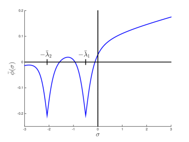
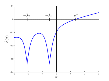
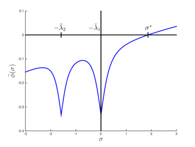
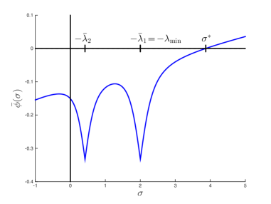
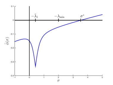
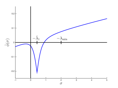
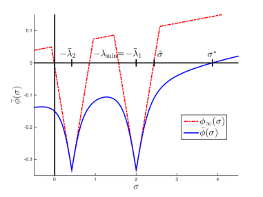
Note that $\bar{\phi}^{\prime}(-\lambda_{j})$ exists as long as $-\lambda_{j}\neq-\bar{\lambda}_{i}$, for $1\leq i\leq\ell$. Furthermore, for $\sigma>-\bar{\lambda}_{1}$, $\bar{\phi}^{\prime}(\sigma)>0$, i.e., $\bar{\phi}(\sigma)$ is strictly increasing on the interval $[-\bar{\lambda}_{1},\infty)$. Finally, it can be shown that $\bar{\phi}^{\prime\prime}(\sigma)<0$ for $\sigma>-\bar{\lambda}_{1}$, i.e., $\bar{\phi}(\sigma)$ is concave on the interval $[-\bar{\lambda}_{1},\infty)$. For illustrative purposes, we plot examples of $\bar{\phi}(\sigma)$ in Fig. 1 for the different cases we considered in this Section 3. Note that we use Newton’s method to find $\sigma^{*}$ when (a) $\lambda_{\min}\geq 0$ and $\bar{\phi}(0)$ (see Figs. 1(b) and (c)), or (b) $\lambda_{\min}<0$ and $\bar{\phi}(-\lambda_{\min})<0$ (see Figs. 1(d) and (e)).

(a)	(b)
(c)	(d)
(e)	(f)

Figure 1. Graphs of the function $\bar{\phi}(\sigma)$. (a) The positive-definite case where the unconstrained minimizer is within the trust-region radius, i.e., $\bar{\phi}(0)\geq 0$, and $\sigma^{*}=0$. (b) The positive-definite case where the unconstrained minimizer is infeasible, i.e., $\bar{\phi}(0)<0$. (c) The singular case where $\bar{\lambda}_{1}=\lambda_{\text{min}}=0$. (d) The indefinite case where $\bar{\lambda}_{1}=\lambda_{\text{min}}<0$. (e) When the coefficients $a_{i}$ corresponding to $\lambda_{\text{min}}$ are all 0, $\bar{\phi}(\sigma)$ does not have a singularity at $\lambda_{\text{min}}$. Note that this case is not the hard case since $\bar{\phi}(-\lambda_{\min})<0$. (f) The hard case where there does not exist $\sigma^{*}>-\lambda_{\text{min}}$ such that $\bar{\phi}(\sigma^{*})=0$.

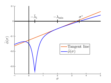
We now define an initial iterate such that Newton’s method is guaranteed to converge to $\sigma^{*}$ monotonically.

Theorem 3.

Suppose $\bar{\phi}(\max\{0,-\lambda_{\min}\})<0$. Let

$$\hat{\sigma}\mathop{\,{\scriptstyle\stackrel{{\scriptstyle\triangle}}{{=}}}}\,\max_{1\leq i\leq k+2}\left\{\frac{|a_{i}|}{\delta}-\lambda_{i}\right\}=\frac{|a_{j}|}{\delta}-\lambda_{j}$$ (18)

for some $1\leq j\leq k+2$. Newton’s method applied to $\bar{\phi}(\sigma)$ with initial iterate $\sigma^{(0)}\mathop{\,{\scriptstyle\stackrel{{\scriptstyle\triangle}}{{=}}}}\,\max\{0,\hat{\sigma}\}$ is guaranteed to converge to $\sigma^{*}$ monotonically.

Proof.

Since $\bar{\phi}(\sigma)$ is strictly increasing and concave on $[-\lambda_{\min},\infty)$ and $\bar{\phi}(\sigma^{*})=0$, it is sufficient to show that (i) $-\lambda_{\min}\leq\sigma^{(0)}\leq\sigma^{*}$, and (ii) $\bar{\phi}^{\prime}(\sigma^{(0)})$ exists (see e.g., [17]).

We note that $\hat{\sigma}\geq-\lambda_{\min}$, and thus, $\sigma^{(0)}\geq\max\{0,-\lambda_{\min}\}\geq-\lambda_{\min}$. To show that $\sigma^{(0)}\leq\sigma^{*}$, we show that $\bar{\phi}(\sigma^{(0)})\leq\bar{\phi}(\sigma^{*})=0$.

If $\hat{\sigma}=|a_{j}|/\delta-\lambda_{j}$ with $|a_{j}|\neq 0$, then evaluating $\|p(\sigma)\|$ at $\sigma=\hat{\sigma}$ yields

$$\|p(\hat{\sigma})\|^{2}\ =\ \sum_{i=1}^{k+2}\frac{a_{i}^{2}}{(\lambda_{i}+\hat{\sigma})^{2}}\\ \ \geq\ \frac{a_{j}^{2}}{(\lambda_{j}+\hat{\sigma})^{2}}\\ \ =\ \frac{a_{j}^{2}}{(\lambda_{j}+\frac{|a_{j}|}{\delta}-\lambda_{j})^{2}}\\ \ =\ \delta^{2},$$

and thus, $\bar{\phi}(\hat{\sigma})\leq 0$. Since $\bar{\phi}(\max\{0,-\lambda_{\min}\})<0$, then $\bar{\phi}(\sigma^{(0)})\leq 0$. If $|a_{j}|=0$, then $\hat{\sigma}=-\lambda_{j}$. Since $-\lambda_{i}\leq-\lambda_{\min}$ for all $i$, $\hat{\sigma}=-\lambda_{\min}$. Thus, $\bar{\phi}(\sigma^{(0)})=\bar{\phi}(\max\{0,-\lambda_{\min}\})<0$. Consequently, $\bar{\phi}(\sigma^{(0)})\leq 0$, and therefore, $\sigma^{(0)}\leq\sigma^{*}$ since $\bar{\phi}(\sigma)$ is monotonically increasing.

Next, we show that $\bar{\phi}^{\prime}(\sigma^{(0)})$ exists. On the interval $(-\lambda_{\min},\infty)$, $\bar{\phi}(\sigma)$ is differentiable (see (17)). Therefore, if $\sigma^{(0)}>-\lambda_{\min}$, then $\bar{\phi}^{\prime}(\sigma^{(0)})$ exists. If $\sigma^{(0)}=-\lambda_{\min}$, then $\hat{\sigma}=-\lambda_{\min}$, which implies that $a_{1}=\cdots=a_{r}=0$ or $a_{k+2}$ = 0 (see (18)). From the definition of $\bar{\phi}(\sigma)$, $\lambda_{\min}\neq\bar{\lambda}_{i}$ for $1\leq i\leq\ell$. Thus, $\bar{\phi}(\sigma)$ is differentiable at $\sigma=-\lambda_{\min}=\sigma^{(0)}$. $\square$

∎

We note that when $a_{j}\neq 0$ in (18), $\hat{\sigma}$ is the largest $\sigma$ that solves the secular equation with the infinity norm:

$$\phi_{\infty}(\hat{\sigma})=\frac{1}{\|v(\hat{\sigma})\|_{\infty}}-\frac{1}{\delta}=0.$$

We illustrate the choice of initial iterate for Newton’s method in Fig. 2.

(a)	(b)

Figure 2. Choice of initial iterate for Newton’s method. (a) If $a_{j}\neq 0$ in (18), then $\hat{\sigma}$ corresponds to the largest root of $\phi_{\infty}(\sigma)$ (in red). Here, $-\lambda_{\min}>0$, and therefore $\sigma^{(0)}=\hat{\sigma}$. (b) If $a_{j}=0$ in (18), then $\lambda_{\min}\neq\bar{\lambda}_{1}$, and therefore, $\bar{\phi}(\sigma)$ is differentiable at $-\lambda_{\min}$ since $\bar{\phi}(\sigma)$ is differentiable on $(-\bar{\lambda}_{1},\infty)$. Here, $-\lambda_{\min}>0$, and thus, $\sigma^{(0)}=\hat{\sigma}=-\lambda_{\min}$.

Finally, we present Newton’s method for computing $\sigma^{*}$.

Define tolerance $\tau>0$;

if $\bar{\phi}(\max\{0,-\lambda_{\min}\})<0$ then

      $\hat{\sigma}=\max_{1\leq j\leq k+2}\frac{|a_{j}|}{\delta}-\lambda_{j}$;

      $\sigma=\max\{0,\hat{\sigma}\}$;

      while $|\bar{\phi}(\sigma)|>\tau$ do

           $\sigma=\sigma-\bar{\phi}(\sigma)/\bar{\phi}^{\prime}(\sigma)$;

           end while

          $\sigma^{*}=\sigma$;

           else if $\lambda_{\min}<0$ then

               $\sigma^{*}=-\lambda_{\min}$;

                else

                     $\sigma^{*}=0$;

                     end if

ALGORITHM 2 Newton’s method for computing $\sigma^{*}$

4. Numerical experiments

In this section, we demonstrate the accuracy of the proposed OBS algorithm implemented in MATLAB to solve limited-memory SR1 trust-region subproblems. For the experiments, five sets of experiments composed of problems of various sizes were generated using random data. The Newton method to find a root of $\phi$ was terminated when the $i$th iterate satisfied $\|\phi(\sigma^{(i)})\|\leq\|\phi(\sigma^{(0)})\|+\tau$, where $\sigma^{(0)}$ denotes the initial iterate for Newton’s method and $\tau=1.0\times 10^{-10}$. This is the only stopping criteria used by the OBS method since other aspects of this method compute solutions by formula. The problem sizes $n$ range from $n=10^{3}$ to $n=10^{7}$. The number of limited-memory updates $k$ was set to 4, and thus $k+1=5$, and $\gamma=0.5$ unless otherwise specified below. The pairs $S$ and $Y$, both $n\times(k+1)$ matrices, were generated from random data. Finally, $g$ was generated by random data unless otherwise stated. The five sets of experiments are intended to be comprehensive: They include the unconstrained case and the three cases discussed in Section 3. The five experiments are as follows:

1. The matrix $B$ is positive definite with $\|p_{u}\|\leq\delta$: We ensure $\Psi$ and $M$ are such that $B$ is strictly positive definite by altering the spectral decomposition of $RMR^{T}$. We choose $\delta=\mu\|p_{u}\|$, where $\mu=1.25$, to guarantee that the unconstrained minimizer is feasible. The graph of $\bar{\phi}(\sigma)$ corresponding to this case is illustrated in Fig. 1(a).

2. The matrix $B$ is positive definite with $\|p_{u}\|>\delta$: We ensure $\Psi$ and $M$ are such that $B$ is strictly positive definite by altering the spectral decomposition of $RMR^{T}$. We choose $\delta=\mu\|p_{u}\|$, where $\mu$ is randomly generated between 0 and 1, to guarantee that the unconstrained minimizer is infeasible. The graph of $\bar{\phi}(\sigma)$ corresponding to this case is illustrated in Fig. 1(b).

3. The matrix $B$ is positive semidefinite and singular with $p=-B^{\dagger}g$ infeasible: We ensure $\Psi$ and $M$ are such that $B$ is positive semidefinite and singular by altering the spectral decomposition of $RMR^{T}$. Two cases are tested: (a) $\bar{\phi}(0)<0$ and (b) $\bar{\phi}(0)\geq 0$. Case (a) occurs when $\delta=(1+\mu)\|p_{u}\|$, where $\mu$ is randomly generated between 0 and 1; case (b) occurs when $\delta=\mu\|p_{u}\|$, where $\mu$ is randomly generated between 0 and 1. The graph of $\bar{\phi}(\sigma)$ in case (a) corresponds to Fig. 1(c). In case (b), $a_{i}=0$ for $i=1,\dots,r$, and thus, $\bar{\phi}(\sigma)$ does not have a singularity at $\sigma=0$, implying the graph of $\bar{\phi}(\sigma)$ for this case corresponds to Fig 1̇(a).

4. The matrix $B$ is indefinite with $\bar{\phi}(-\lambda_{\min})<0$: We ensure $\Psi$ and $M$ are such that $B$ is indefinite by altering the spectral decomposition of $RMR^{T}$. We test two subcases: (a) the vector $g$ is generated randomly, and (b) a random vector $g$ is projected onto the orthogonal complement of ${P_{\parallel}}_{1}\in\Re^{n\times r}$ so that $a_{i}=0,i=1,\ldots,r$, where $r=2$. For case (b), $\delta=\mu\|p_{u}\|$, where $\mu$ is randomly generated between 0 and 1, so that $\bar{\phi}(-\lambda_{\min})<0$. The graph of $\bar{\phi}(\sigma)$ in case (a) corresponds to Fig. 1(d), and $\bar{\phi}(\sigma)$ in case (b) corresponds to Fig. 1(e).

5. The hard case ($B$ is indefinite): We ensure $\Psi$ and $M$ are such that $B$ is indefinite by altering the spectral decomposition of $RMR^{T}$. We test two subcases: (a) $\lambda_{\min}=\lambda_{1}=\hat{\lambda}_{1}+\gamma<0$, and (b) $\lambda_{\min}=\gamma<0$. In both cases, $\delta=(1+\mu)\|p_{u}\|$, where $\mu$ is randomly generated between 0 and 1, so that $\bar{\phi}(-\lambda_{\min})>0$. The graph of $\bar{\phi}(\sigma)$ for both cases of the hard case corresponds to Fig. 1(f).

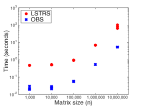
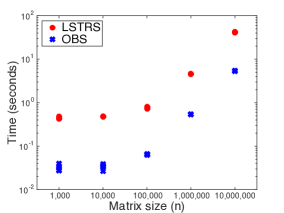
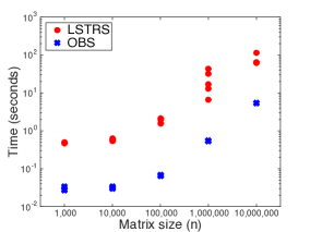
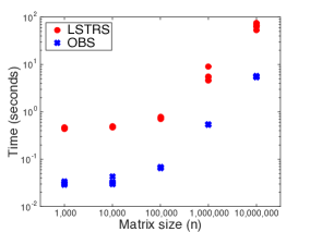
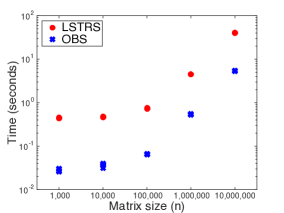
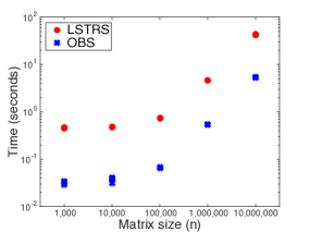
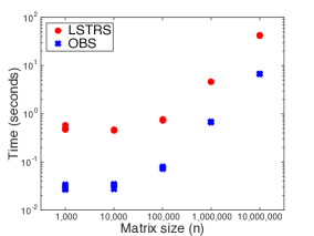
We report the following: (1) opt 1 (abs)=$\|(B+\sigma^{*}I)p^{*}+g\|$, which corresponds to the norm of the error in the first optimality conditions; (2) opt 1 (rel) =$(\|(B+\sigma^{*}I)p^{*}+g\|)/\|g\|$, which corresponds to the norm of the relative error in the first optimality conditions; (3) opt 2=$\sigma^{*}|p^{*}-\delta|$, which corresponds to the absolute error in the second optimality conditions; (4) $|\phi(\sigma^{*})|$, which measures how well the secular equation is satisfied; and (5) Time. We ran each experiment five times and report one representative result for each experiment. We show in Fig. 3 the computational time for each of the five runs in each experiment.

For comparison, we report results for the OBS method as well as the LSTRS method [20, 21]. The LSTRS method solves large trust-region subproblems by converting the subproblems into parametrized eigenvalue problems. This method uses only matrix-vector products. For these tests, we suppressed all run-time output of the LSTRS method and supplied a routine to compute matrix-vector products using the factors in the compact formulation (see (5)), i.e., given a vector $v$, the product with $B$ is computed as $Bv\leftarrow\gamma v+\Psi(M(\Psi^{T}v)).$ Note that the computations of $M$ and $\Psi$ are not included in the time counts for LSTRS.

Table 1. Experiment 1: OBS method with $B$ is positive definite and $\|p_{u}\|\leq\delta$.

$n$	opt 1 (abs)	opt 1 (rel)	opt 2	$\sigma^{*}$	Time
1.0e+03	3.24e-15	1.03e-16	0.00e+00	0.00e+00	2.12e-02
1.0e+04	1.21e-14	1.21e-16	0.00e+00	0.00e+00	2.76e-02
1.0e+05	4.61e-14	1.46e-16	0.00e+00	0.00e+00	5.46e-02
1.0e+06	1.08e-13	1.08e-16	0.00e+00	0.00e+00	5.34e-01
1.0e+07	5.31e-13	1.68e-16	0.00e+00	0.00e+00	5.34e+00

Table 2. Experiment 1: LSTRS method with $B$ is positive definite and $\|p_{u}\|\leq\delta$.

$n$	opt 1 (abs)	opt 1 (rel)	opt 2	$\sigma^{*}$	Time
1.0e+03	2.11e-05	6.70e-07	0.00e+00	0.00e+00	4.72e-01
1.0e+04	8.27e-07	8.28e-09	0.00e+00	0.00e+00	4.98e-01
1.0e+05	2.64e-07	8.37e-10	0.00e+00	0.00e+00	9.15e-01
1.0e+06	3.54e-09	3.53e-12	0.00e+00	0.00e+00	7.08e+00
1.0e+07	2.79e-09	8.81e-13	0.00e+00	0.00e+00	6.66e+01

Tables 1 and 2 shows the results of Experiment 1. In all cases, the OBS method and the LSTRS method found global solutions of the trust-region subproblems. The relative error in the OBS method is smaller than the relative error in the LSTRS method. Moreover, the OBS method solved each subproblem in less time than the LSTRS method.

Table 3. Experiment 2: OBS method with $B$ is positive definite and $\|p_{u}\|>\delta$.

$n$	opt 1 (abs)	opt 1 (rel)	opt 2	$\sigma^{*}$	Time
1.0e+03	3.44e-15	1.06e-16	1.75e-09	4.82e+01	2.83e-02
1.0e+04	1.35e-14	1.35e-16	5.83e-13	1.99e+01	2.70e-02
1.0e+05	3.34e-14	1.06e-16	6.15e-13	1.57e+01	6.39e-02
1.0e+06	9.58e-14	9.58e-17	1.30e-11	7.06e+01	5.38e-01
1.0e+07	4.49e-13	1.42e-16	5.39e-06	1.08e+00	5.37e+00

Table 4. Experiment 2: LSTRS method with $B$ is positive definite and $\|p_{u}\|>\delta$.

$n$	opt 1 (abs)	opt 1 (rel)	opt 2	$\sigma^{*}$	Time
1.0e+03	1.32e-14	4.05e-16	6.25e-04	4.82e+01	4.44e-01
1.0e+04	1.20e-13	1.20e-15	1.20e-03	1.99e+01	4.80e-01
1.0e+05	5.45e-11	1.73e-13	4.90e-04	1.57e+01	7.30e-01
1.0e+06	4.68e-10	4.68e-13	1.35e-06	7.06e+01	4.56e+00
1.0e+07	4.15e-05	1.31e-08	4.47e-05	1.08e+00	4.21e+01

Tables 3 and 4 show the results of Experiment 2. In this case, the unconstrained minimizer is not inside the trust region, making the value of $\sigma^{*}$ strictly positive. As in the first experiment, the OBS method appears to obtain solutions to higher accuracy (columns 1, 2, and 3) and in less time (column 4) than the LSTRS method. Finally, it is worth noting that as $n$ increases, the accuracy of the solutions obtained by the LSTRS method appears to degrade.

Table 5. Experiment 3(a): OBS method with $B$ is positive semidefinite and singular with $\|B^{\dagger}g\|>\delta$.

$n$	opt 1 (abs)	opt 1 (rel)	opt 2	$\sigma^{*}$	Time
1.0e+03	2.80e-14	8.89e-16	6.25e-10	3.38e-01	2.70e-02
1.0e+04	1.17e-13	1.16e-15	1.18e-08	1.03e-01	3.36e-02
1.0e+05	3.48e-12	1.10e-14	2.16e-07	8.75e-03	6.43e-02
1.0e+06	1.44e-11	1.44e-14	1.48e-09	3.62e-03	5.44e-01
1.0e+07	5.52e-10	1.74e-13	8.96e-09	2.88e-03	5.39e+00

Table 6. Experiment 3(a): LSTRS method with $B$ is positive semidefinite and singular with $\|B^{\dagger}g\|>\delta$.

$n$	opt 1 (abs)	opt 1 (rel)	opt 2	$\sigma^{*}$	Time
1.0e+03	9.75e-03	3.10e-04	1.51e-16	3.41e-01	4.78e-01
1.0e+04	7.93e-02	7.91e-04	2.65e-15	1.07e-01	5.69e-01
1.0e+05	1.85e-01	5.84e-04	8.16e-16	9.57e-03	1.56e+00
1.0e+06	1.29e-01	1.29e-04	6.04e-16	1.70e-03	1.28e+01
1.0e+07	2.24e+03	7.09e-01	1.05e-10	1.30e-06	6.39e+01

Tables 5 and 6 display the results of Experiment 3(a). This is experiment is the first of two in which $B$ is highly ill-conditioned. In this experiment, the LSTRS method appears unable to obtain solutions to high absolute accuracy (see column 2 in Table 6). Moreover, the time required by the LSTRS to obtain solutions is, in some cases, significantly more than the time required by the OBS method. In contrast, the OBS method is able to obtain high accuracy solutions. Notice that the optimal values $\sigma^{*}$ found by both methods appear to differ. Global solutions to the subproblems solved in Experiment 3(a) lie on the boundary of the trust region. Because LSTRS was able to satisfy the second optimality condition to high accuracy but not the first, this suggests LSTRS’s solution $p^{*}$ lies on the boundary but there is some error in this solution. As $n$ increases, the solution quality of the LSTRS method appears to decline with significant error in the case of $n=10^{7}$. In this experiment, the OBS method appears to find solutions to high accuracy in comparable time to other experiments; in contrast, the LSTRS method appears to have difficulty finding global solutions.

Table 7. Experiment 3(b): OBS method with $B$ is positive semidefinite and singular with $\|B^{\dagger}g\|\leq\delta$.

$n$	opt 1 (abs)	opt 1 (rel)	opt 2	$\sigma^{*}$	Time
1.0e+03	4.10e-15	1.34e-16	9.05e-10	4.85e+01	3.01e-02
1.0e+04	1.01e-14	1.02e-16	1.34e-11	6.98e+00	4.36e-02
1.0e+05	3.03e-14	9.55e-17	7.99e-14	2.25e+01	6.70e-02
1.0e+06	1.39e-13	1.39e-16	4.18e-12	3.42e+00	5.41e-01
1.0e+07	3.46e-13	1.09e-16	1.28e-11	1.08e+00	5.37e+00

Table 8. Experiment 3(b): LSTRS method with $B$ is positive semidefinite and singular with $\|B^{\dagger}g\|\leq\delta$.

$n$	opt 1 (abs)	opt 1 (rel)	opt 2	$\sigma^{*}$	Time
1.0e+03	9.40e-15	2.97e-16	8.19e-04	4.85e+01	4.42e-01
1.0e+04	2.06e-12	2.07e-14	6.59e-04	6.98e+00	4.79e-01
1.0e+05	1.69e-11	5.34e-14	4.27e-05	2.25e+01	7.43e-01
1.0e+06	6.27e-08	6.28e-11	6.19e-05	3.42e+00	4.60e+00
1.0e+07	4.28e-05	1.35e-08	2.59e-05	1.08e+00	6.29e+01

The results for Experiment 3(b) are shown in Tables 7 and 8. This is the second experiment involving ill-conditioned matrices. As with Experiment 3(a), the OBS method is able to obtain high-accuracy solutions in generally less time than the LSTRS method. The accuracy obtained by the LSTRS method appears to degrade as the size of the problem increases. In this experiment, the global solution always lies on the boundary, but the larger residuals associated the second optimality condition in Table 8 indicate that the computed solutions by LSTRS do not lie on the boundary.

Table 9. Experiment 4(a): OBS method with $B$ is indefinite with $\bar{\phi}(-\lambda_{\min})<0$. The vector $g$ is randomly generated.

$n$	opt 1 (abs)	opt 1 (rel)	opt 2	$\sigma^{*}$	Time
1.0e+03	2.83e-15	9.04e-17	3.57e-12	1.89e+02	3.05e-02
1.0e+04	1.27e-14	1.27e-16	1.53e-09	1.18e+02	3.99e-02
1.0e+05	3.42e-14	1.08e-16	9.15e-13	3.92e+02	6.40e-02
1.0e+06	1.19e-13	1.20e-16	4.79e-12	5.39e+03	5.43e-01
1.0e+07	3.46e-13	1.09e-16	8.18e-11	1.94e+04	5.35e+00

Table 10. Experiment 4(a): LSTRS method with $B$ is indefinite with $\bar{\phi}(-\lambda_{\min})<0$. The vector $g$ is randomly generated.

$n$	opt 1 (abs)	opt 1 (rel)	opt 2	$\sigma^{*}$	Time
1.0e+03	4.92e-14	1.57e-15	5.40e-04	1.89e+02	4.40e-01
1.0e+04	2.82e-14	2.79e-16	1.03e-03	1.18e+02	4.80e-01
1.0e+05	2.11e-13	6.69e-16	2.68e-06	3.92e+02	7.24e-01
1.0e+06	2.93e-11	2.94e-14	1.38e-07	5.39e+03	4.49e+00
1.0e+07	1.81e-10	5.74e-14	3.19e-10	1.94e+04	4.12e+01

The results for Experiment 4(a) are displayed in Tables 9 and 10. Both methods found solutions that satisfied the first optimality conditions to high accuracy. The overall solution quality from the OBS method appears better in the sense that the residuals for both optimality conditions in Table 9 are smaller than the residuals for both optimality conditions in Table 10. Finally, the OBS method took less time to solve the subproblem than the LSTRS method.

Table 11. Experiment 4(b): OBS method with $B$ is indefinite with $\bar{\phi}(-\lambda_{\min})<0$. The vector $g$ lies in the orthogonal complement of ${P_{\parallel}}_{1}$.

$n$	opt 1 (abs)	opt 1 (rel)	opt 2	$\sigma^{*}$	Time
1.0e+03	3.42e-15	1.07e-16	1.17e-09	1.31e+01	2.91e-02
1.0e+04	1.38e-14	1.38e-16	1.50e-14	2.81e+00	3.16e-02
1.0e+05	3.17e-14	1.00e-16	3.55e-13	1.82e+01	6.66e-02
1.0e+06	1.30e-13	1.30e-16	1.76e-12	4.76e+00	5.46e-01
1.0e+07	3.14e-13	9.94e-17	4.36e-11	7.58e+01	5.36e+00

Table 12. Experiment 4(b): LSTRS method with $B$ is indefinite with $\bar{\phi}(-\lambda_{\min})<0$. The vector $g$ lies in the orthogonal complement of ${P_{\parallel}}_{1}$.

$n$	opt 1 (abs)	opt 1 (rel)	opt 2	$\sigma^{*}$	Time
1.0e+03	1.16e-14	3.64e-16	1.24e-03	1.31e+01	4.42e-01
1.0e+04	2.48e-12	2.49e-14	1.02e-04	2.81e+00	4.70e-01
1.0e+05	1.50e-10	4.75e-13	2.82e-04	1.82e+01	7.30e-01
1.0e+06	1.65e-08	1.65e-11	9.70e-05	4.76e+00	4.65e+00
1.0e+07	2.08e-07	6.58e-11	1.06e-05	7.58e+01	4.21e+01

The results of Experiment 4(b) are in Tables 11 and 12. Both methods solved the subproblem to high accuracy as measured by the first optimality condition; however, the OBS method solved the subproblem to significantly better accuracy as measured by the second optimality condition than the LSTRS method. All residual associated with the first and second optimality condition are less for the solution obtained by the OBS method. Moreover, the time required to find solutions was less for the OBS method.

Table 13. Experiment 5(a): The OBS method in the hard case ($B$ is indefinite) and $\lambda_{\min}=\lambda_{1}=\hat{\lambda}_{1}+\gamma<0$.

$n$	opt 1 (abs)	opt 1 (rel)	opt 2	$\sigma^{*}$	Time
1.0e+03	1.29e-14	4.34e-16	1.93e-16	4.35e-01	3.38e-02
1.0e+04	5.87e-14	5.86e-16	2.59e-14	6.08e-01	2.73e-02
1.0e+05	2.34e-12	7.43e-15	5.79e-14	8.15e+00	8.08e-02
1.0e+06	1.33e-11	1.33e-14	1.19e-12	3.97e+00	6.72e-01
1.0e+07	1.67e-10	5.28e-14	4.43e-12	5.27e-01	6.71e+00

Table 14. Experiment 5(a): The LSTRS method in the hard case ($B$ is indefinite) and $\lambda_{\min}=\lambda_{1}=\hat{\lambda}_{1}+\gamma<0$.

$n$	opt 1 (abs)	opt 1 (rel)	opt 2	$\sigma^{*}$	Time
1.0e+03	2.10e-05	7.07e-07	1.16e-15	4.35e-01	4.70e-01
1.0e+04	3.88e+00	3.87e-02	1.50e-03	6.08e-01	4.71e-01
1.0e+05	1.27e+02	4.01e-01	5.72e-04	8.15e+00	7.65e-01
1.0e+06	2.04e+02	2.04e-01	1.45e-04	3.97e+00	4.59e+00
1.0e+07	1.64e+03	5.17e-01	2.30e-05	5.27e-01	4.23e+01

In the hard case with $\lambda_{\min}$ being a nontrivial eigenvalue, the OBS method was obtain global solutions to the subproblems; however, the LSTRS had difficulty finding high-accuracy solutions for all problem sizes. In particular, as $n$ increases, the solution quality of the LSTRS method appears to decline with significant error in the case of $n=10^{7}$. In all cases, the time required by the OBS method to find a solution was less than that of the time required by the LSTRS method.

Table 15. Experiment 5(b): The OBS method in the hard case ($B$ is indefinite) and $\lambda_{\min}=\gamma<0$.

$n$	opt 1 (abs)	opt 1 (rel)	opt 2	$\sigma^{*}$	Time
1.0e+03	3.52e-15	1.11e-16	3.53e-09	6.35e+01	2.93e-02
1.0e+04	9.50e-15	9.48e-17	1.16e-14	2.10e+02	3.82e-02
1.0e+05	3.01e-14	9.50e-17	4.49e-13	4.49e+02	6.71e-02
1.0e+06	9.48e-14	9.47e-17	6.86e-12	1.34e+04	5.32e-01
1.0e+07	3.40e-13	1.07e-16	2.97e-12	8.91e+03	5.36e+00

Table 16. Experiment 5(b): The LSTRS method in the hard case ($B$ is indefinite) and $\lambda_{\min}=\gamma<0$.

$n$	opt 1 (abs)	opt 1 (rel)	opt 2	$\sigma^{*}$	Time
1.0e+03	2.24e-14	7.12e-16	7.36e-04	6.35e+01	4.41e-01
1.0e+04	6.35e-14	6.33e-16	1.92e-06	2.10e+02	5.02e-01
1.0e+05	2.26e-13	7.14e-16	5.09e-08	4.49e+02	7.49e-01
1.0e+06	6.61e-12	6.61e-15	4.76e-08	1.34e+04	4.32e+00
1.0e+07	8.77e-11	2.77e-14	1.05e-08	8.91e+03	4.09e+01

The results of Experiment 5(b) are in Tables 15 and 16. Unlike in Experiment 5(a), the LSTRS method was able to find solutions to high accuracy. In all cases, the OBS method was able to find solutions with higher accuracy than the LSTRS method and in less time.

Experiment 1	Experiment 2
Experiment 3(a)	Experiment 3(b)
Experiment 4(a)	Experiment 4(b)
Experiment 5(a)	Experiment 5(b)

Figure 3. Semi-log plots of the computational times (in seconds). Each experiment was run five times; computational time for the LSTRS and OBS method are shown for each run. In all cases, the OBS method outperforms LSTRS in terms of computational time.

5. Concluding remarks

In this paper, we presented the OBS method, which solves trust-region subproblems of the form (1) where $B$ is a large L-SR1 matrix. The OBS method uses two main strategies. In one strategy, $\sigma^{*}$ is computed from Newton’s method and initialized at a point where Newton’s method is guaranteed to converge monotonically to $\sigma^{*}$. With $\sigma^{*}$ in hand, $p^{*}$ is computed directly by formula. For the other strategy, we propose a method that relies on an orthonormal basis to directly compute $p^{*}$. (In this case, $\sigma^{*}$ can be determined from the spectral decomposition of $B$.) Numerical experiments suggest that the OBS method is able to solve large L-SR1 trust-region subproblems to high accuracy. Moreover, the method appears to be more robust than the LSTRS method, which does not exploit the specific structure of $B$. In particular, the proposed OBS method achieves high accuracy in less time in all of the experiments and in all measures of optimality than the LSTRS method. Future research will consider the best implementation of the OBS method in a trust-region method (see, for example, [3]), including initialization of $\gamma$ and rules for updating the matrices $S$ and $Y$ containing the quasi-Newton pairs.

6. Acknowledgments

This research is support in part by National Science Foundation grants CMMI-1333326 and CMMI-1334042.

References

- [1] O. Burdakov, L. Gong, Y.-X. Yuan, and S. Zikrin. On efficiently combining limited memory and trust-region techniques. Technical Report 2013:13, Link ping University, Optimization, 2015.
- [2] J. V. Burke, A. Wiegmann, and L. Xu. Limited memory BFGS updating in a trust-region framework. Technical report, University of Washington, 1996.
- [3] R. H. Byrd, H. F. Khalfan, and R. B. Schnabel. Analysis of a symmetric rank-one trust region method. SIAM Journal on Optimization, 6(4):1025–1039, 1996.
- [4] R. H. Byrd, J. Nocedal, and R. B. Schnabel. Representations of quasi-Newton matrices and their use in limited-memory methods. Math. Program., 63:129–156, 1994.
- [5] A. R. Conn, N. I. M. Gould, and P. L. Toint. Convergence of quasi-newton matrices generated by the symmetric rank one update. Math. Program., 50(2):177–195, Mar. 1991.
- [6] A. R. Conn, N. I. M. Gould, and P. L. Toint. Trust-Region Methods. Society for Industrial and Applied Mathematics (SIAM), Philadelphia, PA, 2000.
- [7] J. B. Erway and P. E. Gill. A subspace minimization method for the trust-region step. SIAM Journal on Optimization, 20(3):1439–1461, 2010.
- [8] J. B. Erway, P. E. Gill, and J. D. Griffin. Iterative methods for finding a trust-region step. SIAM Journal on Optimization, 20(2):1110–1131, 2009.
- [9] J. B. Erway and R. F. Marcia. Algorithm 943: MSS: MATLAB software for L-BFGS trust-region subproblems for large-scale optimization. ACM Transactions on Mathematical Software, 40(4):28:1–28:12, June 2014.
- [10] J. B. Erway and R. F. Marcia. On efficiently computing the eigenvalues of limited-memory quasi-newton matrices. SIAM Journal on Matrix Analysis and Applications, 36(3):1338–1359, 2015.
- [11] D. M. Gay. Computing optimal locally constrained steps. SIAM J. Sci. Statist. Comput., 2(2):186–197, 1981.
- [12] I. Griva, S. G. Nash, and A. Sofer. Linear and Nonlinear Optimization. Society for Industrial and Applied Mathematics, Philadelphia, 2009.
- [13] W. W. Hager. Minimizing a quadratic over a sphere. SIAM J. Optim., 12(1):188–208, 2001.
- [14] W. W. Hager and S. Park. Global convergence of SSM for minimizing a quadratic over a sphere. Math. Comp., 74(74):1413–1423, 2004.
- [15] C. Kelley and E. Sachs. Local convergence of the symmetric rank-one iteration. Computational Optimization and Applications, 9(1):43–63, 1998.
- [16] H. F. Khalfan, R. H. Byrd, and R. B. Schnabel. A theoretical and experimental study of the symmetric rank-one update. SIAM Journal on Optimization, 3(1):1–24, 1993.
- [17] D. R. Kincaid and E. W. Cheney. Numerical analysis: mathematics of scientific computing, volume 2. American Mathematical Soc., 2002.
- [18] J. J. Moré and D. C. Sorensen. Computing a trust region step. SIAM J. Sci. and Statist. Comput., 4:553–572, 1983.
- [19] J. Nocedal and S. J. Wright. Numerical Optimization. Springer-Verlag, New York, 1999.
- [20] M. Rojas, S. A. Santos, and D. C. Sorensen. A new matrix-free algorithm for the large-scale trust-region subproblem. SIAM Journal on optimization, 11(3):611–646, 2001.
- [21] M. Rojas, S. A. Santos, and D. C. Sorensen. Algorithm 873: Lstrs: Matlab software for large-scale trust-region subproblems and regularization. ACM Trans. Math. Softw., 34(2):11:1–11:28, Mar. 2008.
- [22] W. Sun and Y.-X. Yuan. Optimization theory and methods: nonlinear programming, volume 1. Springer Science & Business Media, 2006.
- [23] H. Wolkowicz. Measures for symmetric rank-one updates. Mathematics of Operations Research, 19(4):815–830, 1994.