Borraz-Sánchez et al. Convex Relaxations for Gas Expansion Planning

Convex Relaxations for Gas Expansion Planning Conrado Borraz-Sánchez, Russell Bent, Scott Backhaus DSA-4: Energy & Infrastructure Analysis, LANL, Los Alamos, NM-87545, USA

Hassan Hijazi, Pascal Van Hentenryck

NICTA and ANU, Canberra, 260, Australia.

Expansion of natural gas networks is a critical process involving substantial capital expenditures with complex decision-support requirements. Given the non-convex nature of gas transmission constraints, global optimality and infeasibility guarantees can only be offered by global optimisation approaches. Unfortunately, state-of-the-art global optimisation solvers are unable to scale up to real-world size instances. In this study, we present a convex mixed-integer second-order cone relaxation for the gas expansion planning problem under steady-state conditions. The underlying model offers tight lower bounds with high computational efficiency. In addition, the optimal solution of the relaxation can often be used to derive high-quality solutions to the original problem, leading to provably tight optimality gaps and, in some cases, global optimal solutions. The convex relaxation is based on a few key ideas, including the introduction of flux direction variables, exact McCormick relaxations, on/off constraints, and integer cuts. Numerical experiments are conducted on the traditional Belgian gas network, as well as other real larger networks. The results demonstrate both the accuracy and computational speed of the relaxation and its ability to produce high-quality solutions.

1 Introduction

In recent years, the construction of natural gas pipelines has witnessed a tremendous growth on a world-wide level. In the U.S., for instance, a $3 billion expansion project of the gas pipeline system in New England is planned for late 2016. In Europe, the European Investment Bank is supporting a €98 million project for the expansion of gas pipelines in western Poland, to be completed by 2017. These expansion projects aim at increasing gas flow capacity on existing pipeline systems and/or bringing new gas wells into production and commercialization. In addition, the expansion or reinforcement of a pipeline network can also be considered as a risk-awareness strategy to fulfill short or long-term operational management requirements when unforeseen events occur such as component failures or excessive stress and congestion due to extreme weather conditions. These events were observed in New England during the polar vortex experienced in January 2014, when major gas-fired power plants in the northeast of the U.S. were forced to shut down due to mechanical problems and shortages of gas fuel supplies, which drove wholesale power prices up

According to the U.S. Energy Information Administration (EIA), a project for the development and expansion of a Gas Transmission Network (GTN) takes an average of three years from its first announcement until its completion (U.S. Energy Information Administration 2008). The project starts by determining the market needs within an open season exercise where nonbinding agreements of capacity rights are offered to potential customers. The second step consists in developing the expansion design with initial financial commitments from the potential customers. Note that expansions of the gas system include the installation parallel pipelines along existing ones (looping), the conversion of oil pipelines to natural gas pipelines, or the reinforcement of specific pipeline sections.

In this paper, we address the Gas Transmission Network Expansion Planning (GTNEP) problem where the goal is to fulfill projected future gas contracts and to increase the reliability of a gas system under steady-state conditions. A Mixed-Integer NonLinear Programming (MINLP) formulation is proposed to model the design requirements and minimize expansion costs. Given the non-convex nature of the problem, a convex mixed-integer second-order cone relaxation is introduced. The proposed convex relaxation is based on four key ideas: (1) the introduction of variables for modeling the flux directions; (2) exact McCormick relaxations; (3) on/off constraints; and (4) valid integer cuts. Experimental results on the Belgian gas network and a test bed of large-scale synthetic instances demonstrate three key findings:

1. The convex relaxation produces tight lower bounds with high computational efficiency;

2. The solution to the convex relxation can almost always be used to derive high-quality solutions to the original problem, leading to provably tight optimality gaps and, in some cases, global optimal solutions.

3. The proposed approach scales to large-scale instances.

The rest of this paper is organized as follows. Section 2 presents the literature review. Section 3 introduces the problem formulation. Section 4 specifies the convex relaxation. Section 5 presents the computational results and Section 6 concludes the paper.

2 Literature review

The last four decades have seen an interest in natural gas planning problems such as optimal design, optimal reinforcement, and optimal expansion of gas pipeline systems. Algorithms for these problems can be classified in a number of different ways such as exact approaches (Andre et al. 2009, Bonnans et al. 2011, Edgar et al. 1978, 2001b, Wolf 2004) and heuristics (André 2010, Boyd et al. 1994, Humpola et al. 2015, Andre et al. 2009, Humpola and Fügenschuh 2014a). Exact methods include cutting planes (Atamturk 2002, Humpola and Fügenschuh 2014b, Humpola et al. 2015a, Poss 2011) and branch-and-bound (André 2010, Elshiekh et al. 2013, Humpola and Fügenschuh 2015) and they use a variety of commercial (Bakhouya and De Wolf 2008, Elshiekh et al. 2013, Soliman and Murtagh 1982) and open-source (Pfetsch et al. 2012, Uster and Dilaveroglu 2014) solvers. Like this paper, much of the literature relies on approximations and relaxations to improve the tractablity of the underlying planning problems. Examples include continuous relaxations of the discrete design variables (De Wolf and Smeers 1996, Hansen et al. 1991, Soliman and Murtagh 1982) and approximation or relaxations of constraints (Babonneau et al. 2012, Bakhouya and De Wolf 2008, Humpola and Fügenschuh 2015, Poss 2011). Common approaches for implementing these approximations/relaxations include succesive linear programming (De Wolf et al. 1991, Hansen et al. 1991, O’Neill et al. 1979, Wilson et al. 1988) and piecewise linearizations (Correa-Posada and Sánchez-Martín 2014, Markowitz and Manne 1957, Vajda 1964, Zheng et al. 2010).

The contribution of this paper is a novel Second-Order Cone (SOC) relaxation that efficiently addresses the design of large-scale cyclic networks for which flow directions are unknown. The model captures physical, operational, contractual, and on/off constraints and includes models of regular pipelines, valves, short pipes, control valves, compressor stations, and regulators. Its dual solutions can almost always be converted to high-quality or optimal primal solutions. To the best of our knowledge, this combination of features has not appeared in the literature. Our paper focuses on the cost of building the network but can be generalized to include operational costs as well.

We now provide an in-depth review of the most relevant works in the area of natural gas expansion planning problems. One of the earliest papers that addresses natural gas design problems is (Edgar et al. 1978). It focuses on the optimal design of gunbarrel and tree-shaped networks. Their objective minimizes the yearly cumulative operational and investment costs. The optimization variables include pipeline diameters, compression ratios, and the number of compressors. In their later work, Edgar et al. (2001b) present a MINLP formulation for the optimal design of a gas transmission network where the number of compressor stations, the length and diameter of the pipeline sections, and the inlet and outlet pressures at each stations are optimized. They solve a simplified version of the problem in GAMS (GAMS Development Corporation 2008) for a small instance (Edgar et al. 2001a).

Hansen et al. (1991) and Soliman and Murtagh (1982) propose a continuous relaxation for the network design problem. While Hansen et al. (1991) apply a successive linear programming method where a linear subproblem is solved to adjust the discrete choice of diameters, Soliman and Murtagh (1982) apply the commercial NLP solver MINOS Murtagh and Saunders (1998) to handle the relaxed subproblem. O’Neill et al. (1979) and  Wilson et al. (1988) focus on a problem where integer variables are used for the operational state of compressor stations and they also implement a method based on successive linear programming to solve the problem.

De Wolf and Smeers (1996) address the optimal dimensioning of a known pipe network topology with an objective that combines the cost of purchasing gas and the capital expenditures for expansion. The authors formulate the problem as a continuous NLP that selects pipeline diameters and solves the problem by means of a local optimizer. Based on this problem, Wolf (2004) derives conditions under which this problem is convex. Through the use of variational inequality theory, they show convexity of the nonlinear gas flow system under the assumption that the gas net inlet (pressure) is fixed at all supply and demand nodes.  Bakhouya and De Wolf (2008) also present a case study on the same problem with separable transportation and gas objectives that leads to a two-stage problem formulation. In addition to design variables for the optimal pipe diameters, the authors add investment variables representing the maximal power of compressor stations to balance the pipeline construction costs and capital expenditures for increasing power in the compressor units. The authors find an initial solution by solving a convex problem where all pressure constraints are relaxed. Then, the complete problem is locally solved by means of the GAMS/CONOPT solver. In these works, numerical experiments are primarily focused on the Belgian gas transmission network.

Andre et al. (2009) present a MINLP model to solve the investment cost minimization problem for an existing gas system that includes pipelines and regulators and omits compressor stations. The goal is to identify a set of pipeline sections to reinforce and to select an optimal diameter size for these sections based on a discrete set of diameters. Under the assumption that the network is radial (the head loss equations are convex when flows are fixed), the authors propose a continuous relaxation of the pipe diameters (continuous intervals). A branch-and-bound approach for a unique maximal demand scenario is applied to a segment of the French high-pressure natural gas transmission system. A complete review and extensions of these findings are provided in (André 2010).

Babonneau et al. (2009, 2012) focus on the design and operation of a natural gas transmission system while minimizing investment, purchase, and transportation costs. The authors propose an approach based on a minimum energy principle that transforms the non-linear non-convex optimization problem into a convex problem. The underlying convex, bi-objective formulation is an approximation of the investment cost function and the cost of energy to transport the gas. Their continuous formulation is applied to non-divisible constraints such as a limited number of available commercial pipe dimensions.

Bonnans et al. (2011) presents several problems that include the minimization of compressor ratios and the sum of operations and investment costs. The authors propose a global optimization technique that is based on the combination of interval analysis with constraint propagation.

Zheng et al. (2010) discusses different optimization models in the natural gas industry, including the compressor station allocation problem, the least gas purchase problem and optimal dimensioning of gas pipelines. The authors review solution techniques to solve the underlying models which include a piecewise linear programming algorithm and a branch-and-bound algorithm.

Elshiekh et al. (2013) presents a model to optimize the design and operation of the Egyptian gas system, where continuous design variables for the length and diameter of pipelines are considered along with a modified Panhandle equation (Coelho and Pinho 2007). The complete model is directly solved by means of the computer-aided optimization software LINGO (LINDO Systems 1997).

Uster and Dilaveroglu (2014) address the cost minimization problem of designing a new natural gas transmission system and expanding an existing gas system. The authors propose a mathematical formulation to tackle the design/expansion network problem for a given multi-period planning horizon. The underlying MINLP model is formulated in AMPL and solved approximately with Bonmin (Bonami and Lee 2013).

Humpola and Fügenschuh (2014b) and Humpola et al. (2015a) present valid inequalities for a MINLP model of a design problem in gas transmission systems. Different relaxations are applied to the subproblems created after branching on the additive and design variables for the active and passive components. The resulting passive transmission subproblems, which are referred to as leaf problems, admit slack variables to independently relax the pressure domains and the flow conservation constraints. The proposed cutting planes aim at reducing the CPU time of a branch-and-cut-based outer approximation applied to the full model where construction costs are defined by a global constant. Atamturk (2002) and Poss (2011) also propose valid inequalities to reinforce the relaxation approach to the network design structure.

Humpola and Fügenschuh (2015) examines different (convex) relaxations for subproblems created while applying a branch-and-bound technique to a nonlinear network design problem. Cutting planes on the nonlinear potential loss constraints are used to strengthen the relaxed subproblems.

Pfetsch et al. (2012) focuses on the validation of nomination problem while considering regular pipes and valves, control valves, compressors and regulators. The authors describe a two-stage approach to solve the resulting MINLP problem and propose several modeling techniques and approaches to account for, e.g., pressure losses. They also developed several large test cases (GasLib 2014). These problems form the basis for many of the problems we consider in this paper.

3 Problem Formulation

This section derives the problem formulation (as a disjunctive program) in stepwise refinements. It starts by deriving a disjunctive formulation that is then refined by introducing flux variables.

3.1 The Disjunctive Formultion

Gas dynamics along a pipe is described by a set of partial differential equation (PDE) with both spatial and temporal dimensions (Osiadacz 1987, Thorley and Tiley 1987, Sardanashvili 2005):

$$\partial_{t}\rho+\partial_{x}(\rho v)=0,$$ (1)

$$\partial_{t}(\rho v)+\partial_{x}(\rho v^{2})+\partial_{x}p=-\frac{\bm{f}}{2\bm{D}}{\rho v|v|}-{\bm{g}}\sin{\bm{\alpha}}\rho,$$ (2)

$$p=\bm{ZRT}\rho.$$ (3)

Gas velocity $v$, pressure $p$, and density $\rho$ are defined for every point $x$ along the pipe and evolve over time $t$. $\bm{Z}$ represents the gas compressibility factor, $\bm{T}$ the temperature, and $\bm{R}$ the gas constant.

Equation (1) enforces mass conservation, Equation (2) describes momentum balance, and Equation (3) defines the ideal gas thermodynamic relation. In Equation (2), the first term on the right-hand side represents the friction losses in a pipe of diameter $\bm{D}$ with friction factor $\bm{f}$. The second term accounts for the gain or loss of momentum due to gravity $\bm{g}$ if the pipe is tilted by an angle $\bm{\alpha}$. In practice, frictional losses dominate the gravitational term which is dropped. One can also safely assume that the temperature does not fluctuate significantly along a pipe. If temperature gradients are significant, a spatial decomposition, splitting the pipe into temperature stable segments, can be adopted.

Taking into account these assumptions, Equations (1),(2), and (3) are rewritten in terms of pressure $p$ and mass flux $\phi=\rho v$:

$$\partial_{t}p=-\bm{ZRT}\partial_{x}\phi,$$ (4)

$$\partial_{x}p^{2}=-\frac{\bm{fZRT}}{2\bm{D}}\phi|\phi|,$$ (5)

In this work, we assume that the system has reached a steady state after its first commissioning and hence all time derivatives are set to zero. Given this assumption, a Graph Transmission Network (GTN) is represented by a graph $\mathcal{G}=(\mathcal{N},\mathcal{A})$ where $\mathcal{N}$ denotes the set of nodes representing connection points and $\mathcal{A}$ denotes the set of arcs. An arc is a triplet $(a,i,j)$ consisting of a unique identifier $a$ linking nodes $i$ and $j$. For convenience, such a triplet $(a,i,j)$ will be denoted by $a_{ij}$ in the following. Observe that parallel arcs can link the same pair of nodes, e.g., we have arcs $a_{ij}$ and $a^{*}_{ij}$ in a GTN where $a$ and $a^{*}$ are the unique identifiers of these arcs.

By setting the time derivatives to zero, the total gas mass flux along a pipe $a_{ij}$ becomes constant, i.e., $\phi_{i}=\phi_{j}=\phi_{a}$. Hence Equations (4) and (5) simplify to

$$p_{i}^{2}-p_{j}^{2}=\bm{w}_{a}\phi_{a}|\phi_{a}|.$$ (6)

where $\bm{w_{a}}=\frac{\bm{ZR}\bm{f}_{a}\bm{T}_{a}}{{2\bm{D}_{a}}}$.

Gas System Components

The problem formulation considers pipes, compressors, short pipes, resistors, and valves. Compressors, short pipes, and valves are modelled as lossless pipelines, i.e., $\bm{w_{a}}=0$. A compressor installed on arc $a_{ij}$ can increase/decrease the pressure ratio $\alpha_{a}={p_{j}}/{p_{i}}$, within the bounds ${\bm{\alpha}}^{l}_{a}$ and ${\bm{\alpha}}^{u}_{a}$, where ${\bm{\alpha}}^{l}_{a}=1$ and ${\bm{\alpha}}^{u}_{a}\geq 1$ is typical for most compressors. A bi-directional compressor can perform compression based on the flux direction, i.e., it is able to invert the ratio to $\alpha_{a}={p_{i}}/{p_{j}}$ if the flux is going from $j$ to $i$. A standard valve features a binary on/off switch and a control valve has a continuous switching mechanism to adjust pressure. Thus a valve installed on arc $a_{ij}$ can increase/decrease the pressure ratio $\alpha_{a}={p_{j}}/{p_{i}}$, within the bounds ${\bm{\alpha}}^{l}_{a}$ and ${\bm{\alpha}}^{u}_{a}$, where ${\bm{\alpha}}^{l}_{a}>0$ and ${\bm{\alpha}}^{u}_{a}\leq 1$ is typical for most control valves and ${\bm{\alpha}}^{l}_{a}={\bm{\alpha}}^{u}_{a}=1$ for all valves. Finally, a resistor is modelled as a pipeline with a particular (small) loss coefficient ($\bm{w}$).

Expansion Variables

The set of arcs $\mathcal{A}={\cal A}_{e}\cup{\cal A}_{n}$ includes existing arcs ${\cal A}_{e}={\cal P}_{e}~{}\cup~{}{\cal C}_{e}~{}\cup~{}{\cal V}_{e}$, as well as new arcs ${\cal A}_{n}={\cal P}_{n}~{}\cup~{}{\cal C}_{n}$. In this notation, ${\cal P}_{e}$ denotes the set of installed pipelines, resistors, and short pipes. ${\cal C}_{e}$ and ${\cal V}_{e}$ denote the set of existing compressors and valves (control and regular) respectively. ${\cal P}_{n}$ and ${\cal C}_{n}$ denote the set of new pipelines and new compressors respectively. A binary variable $z^{p}_{a}$ is assigned for each new pipe $a_{ij}$ in ${\cal P}_{n}$ to model the expansion decision, i.e., $z^{p}_{a}=1$ if pipeline $a_{ij}$ is installed and $z^{p}_{a}=0$ otherwise. Variables $z^{c}_{ij}$ $((i,j)\in{\cal C}_{n})$ have an equivalent interpretation for new compressors. A binary variable $v_{a}$ is used to control the switching actions of valves.

Disjunctive Formulation

Since the pressure variables only appear in a square form, the formulation uses the variable substitution $\beta_{i}=p_{i}^{2}$ $(i\in\mathcal{N})$. Equations (6) can be written as

$$\beta_{i}-\beta_{j}=\bm{w}_{a}\phi_{a}|\phi_{a}|\;\;\;(a_{ij}\in{\cal P}_{e})$$ (7)

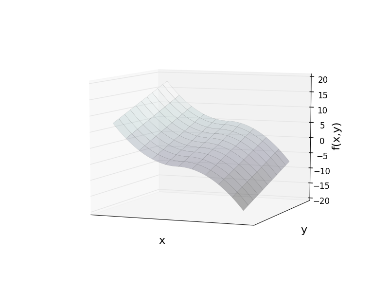
Figure 1 illustrates the curve of the function $f(x,y)=y-{\bm{w}}x|x|$ defined by the pressure drop equation (7).

Figure 1: The Gas Flow Equation $f(x,y)=y-{\bm{w}}x|x|$.

Since bi-directional compressor constraints depend on the flux direction, they can only be modelled using on/off or disjunctive constraints (Hijazi et al. 2010, 2012). i.e.,

$$\begin{cases}\beta_{i}{\bm{\alpha}}^{l}_{a}\leq\beta_{j}\leq\beta_{i}{\bm{\alpha}}^{u}_{a},~{}\text{if }\phi_{a}\geq 0\\ \beta_{j}{\bm{\alpha}}^{l}_{a}\leq\beta_{i}\leq\beta_{j}{\bm{\alpha}}^{u}_{a},~{}\text{if }\phi_{a}\leq 0.\\ \end{cases}$$ (8)

Given a set of injection (resp. demand) nodes ${\cal I}~{}(\text{resp. }{\cal D})\subseteq\mathcal{N}$ with mass flux injection/demand $\bm{q}_{i}$, the problem consists in finding an assignment of the expansion variables $z^{p}_{a}\;(a_{ij}\in{\cal P}_{n})$, node pressures $p_{i}\;(i\in{\cal N})$, and edge flows $\phi_{a}\;(a_{ij}\in{\cal A})$, satisfying the Weymouth equations (7), the compressor constraints (8), and the following node conservation constraints:

$$\sum_{a_{ij}\in{\cal A}}\phi_{a}=\sum_{a_{ji}\in{\cal A}}\phi_{a}+\bm{q}_{i}\;(i\in{\cal N})$$

where $q_{i}=0$ for all $i\in N\setminus({\cal I}\cup{\cal D})$. Note that, in the steady-state model, injections are balanced, i.e., $\sum_{i\in{\cal N}}\bm{q}_{i}=0$. The objective is to minimize the cost of expansion:

$$\min\sum_{a_{ij}\in{\cal P}_{n}}{\bm{c}}_{a}z^{p}_{a}+\sum_{a_{ij}\in{\cal C}_{n}}{\bm{c}}_{a}z^{c}_{a}$$

where ${\bm{c}}_{a}$ represents the cost of installing a new pipeline. The disjunctive formulation of the problem incorporating these ideas is presented in Model 1, where $\bm{\beta^{l}}_{i}=(\bm{\alpha^{l}}_{i})^{2}$ and $\bm{\beta^{u}}_{i}=(\bm{\alpha^{u}}_{i})^{2}$.

Model 1 The Disjunctive Formulation of the GTNEP.

variables:

$$\beta_{i}\in[\bm{\beta^{l}}_{i},\bm{\beta^{u}}_{i}]\;\;\forall i\in\mathcal{N}\mbox{ - squared pressure level variables}$$

$$\phi_{a}\in\mathbb{R}\;\;\forall a_{ij}\in{\cal A}\mbox{ - mass flux on pipe (i,j)}$$

$$z^{p}_{a}\in\{0,1\}\;\;\forall a_{ij}\in{\cal P}_{n}\mbox{ - binary expansion variables for pipes}$$

$$z^{c}_{a}\in\{0,1\}\;\;\forall a_{ij}\in{\cal C}_{n}\mbox{ - binary expansion variables for compressors}$$

$$v_{a}\in\{0,1\}\;\;\forall a_{ij}\in{\cal CV}_{e}\cup{\cal V}_{e}\mbox{ - binary switch variables for valves}$$

objective:

$$\min\sum_{a_{ij}\in{\cal P}_{n}}{\bm{c}}_{a}z^{p}_{a}+\sum_{a_{ij}\in{\cal C}_{n}}{\bm{c}}_{a}z^{c}_{a}$$ (9a)

subject to:

$$\sum_{a_{ij}\in{\cal A}}\phi_{a}=\sum_{a_{ji}\in{\cal A}}\phi_{a}+\bm{q}_{i},~{}\forall i\in{\cal N}$$ (9b)

$$\beta_{i}-\beta_{j}=\bm{w}_{a}\phi_{a}|\phi_{a}|,~{}\forall a_{ij}\in{\cal P}_{e}$$ (9c)

$$z^{p}_{a}(\beta_{i}-\beta_{j})=\bm{w}_{a}\phi_{a}|\phi_{a}|,~{}\forall a_{ij}\in{\cal P}_{n}$$ (9d)

$$\beta_{i}{\bm{\alpha}}^{l}_{a}\leq\beta_{j}\leq\beta_{i}{\bm{\alpha}}^{u}_{a},~{}\text{if }\phi_{a}\geq 0,~{}\forall a_{ij}\in{\cal C}_{e},$$ (9e)

$$\beta_{j}{\bm{\alpha}}^{l}_{a}\leq\beta_{i}\leq\beta_{j}{\bm{\alpha}}^{u}_{a},~{}\text{if }\phi_{a}\leq 0,~{}\forall a_{ij}\in{\cal C}_{e},$$ (9f)

$$\beta_{i}{\bm{\alpha}}^{l}_{a}\leq\beta_{j}\leq\beta_{i}{\bm{\alpha}}^{u}_{a},~{}\text{if }\phi_{a}\geq 0\text{ and }z^{c}_{a}=1,~{}\forall a_{ij}\in{\cal C}_{n},$$ (9g)

$$\beta_{j}{\bm{\alpha}}^{l}_{a}\leq\beta_{i}\leq\beta_{j}{\bm{\alpha}}^{u}_{a},~{}\text{if }\phi_{a}\leq 0\text{ and }z^{c}_{a}=1,~{}\forall a_{ij}\in{\cal C}_{n},$$ (9h)

$$\phi_{a}=0\text{ if }z^{c}_{a}=0,~{}\forall a_{ij}\in{\cal C}_{n}$$ (9i)

$$\beta_{i}{\bm{\alpha}}^{l}_{a}\leq\beta_{j}\leq\beta_{i}{\bm{\alpha}}^{u}_{a},~{}\text{if }\phi_{a}\geq 0\text{ and }v^{c}_{a}=1,~{}\forall a_{ij}\in{\cal V}_{e},$$ (9j)

$$\beta_{j}{\bm{\alpha}}^{l}_{a}\leq\beta_{i}\leq\beta_{j}{\bm{\alpha}}^{u}_{a},~{}\text{if }\phi_{a}\leq 0\text{ and }v^{c}_{a}=1,~{}\forall a_{ij}\in{\cal V}_{e},$$ (9k)

$$\phi_{a}=0\text{ if }v^{c}_{a}=0,~{}\forall a_{ij}\in{\cal C}_{e}$$ (9l)

3.2 The Formulation Based on Flux Direction Variables

This section presents a second formulation using flux direction variables to account for the disjunctive nature of the constraints. For every arc $a_{ij}\in{\mathcal{A}}$, we introduce two binary variables $y^{+}_{a}$ and $y^{-}_{a}\in\{0,1\}$ with the following semantics: $y^{+}_{a}=1$ (resp. $y^{-}_{a}=1$) if the flux moves from $i$ to $j$ (resp. from $j$ to $i$) and 0 otherwise. The mass flux direction is captured by the following system of constraints:

$$\begin{cases}&(1-y^{+}_{a})\sum\limits_{k\in{\cal I}}\bm{q}_{k}\leq\phi_{a}\leq(1-y^{-}_{a})\sum\limits_{k\in{\cal I}}\bm{q}_{k},\\[5.0pt] &\left(1-y^{+}_{a}\right)\bm{\beta^{l}}_{i}\leq\beta_{i}-\beta_{j}\leq\left(1-y^{-}_{a}\right)\bm{\beta^{u}}_{i},\\[5.0pt] &y^{+}_{a}+y^{-}_{a}=1.\\ \end{cases}$$

The first constraint ensures that $y^{+}_{a}=1$ (resp. $y^{-}_{a}=1$) if and only if $\phi_{a}\geq 0$ (resp. $\phi_{a}\leq 0$). Note that $\sum\limits_{k\in{\cal I}}\bm{q}_{k}$ is an upper bound to the mass flux in a pipe. The second constraint enforces a similar condition for the pressure difference. Using the variables and constraints, the pressure drop equation can now be written without absolute value as

$$\left(y^{+}_{a}-y^{-}_{a}\right)(\beta_{i}-\beta_{j})=\bm{w}_{a}\phi_{a}^{2}$$

and the bi-directional compressor constraints are written as

$$\beta_{i}{\bm{\alpha}}^{l}_{a}-(1-y^{+}_{a})(\bm{\beta^{u}}_{i}{\bm{\alpha}}^{l}_{a}-\bm{\beta^{l}}_{j})\leq\beta_{j}\leq\beta_{i}{\bm{\alpha}}^{u}_{a}+(1-y^{+}_{a})(\bm{\beta^{u}}_{j}-\bm{\beta^{l}}_{i}{\bm{\alpha}}^{u}_{a}),~{}\forall a_{ij}\in{\cal C}_{e}$$ (10)

$$\beta_{j}{\bm{\alpha}}^{l}_{a}-(1-y^{-}_{a})(\bm{\beta^{u}}_{j}{\bm{\alpha}}^{l}_{a}-\bm{\beta^{l}}_{i})\leq\beta_{i}\leq\beta_{j}{\bm{\alpha}}^{u}_{a}+(1-y^{-}_{a})(\bm{\beta^{u}}_{i}-\bm{\beta^{l}}_{j}{\bm{\alpha}}^{u}_{a}),~{}\forall a_{ij}\in{\cal C}_{e}$$ (11)

$$\beta_{i}{\bm{\alpha}}^{l}_{a}-(2-y^{+}_{a}-z^{c}_{a})(\bm{\beta^{u}}_{i}{\bm{\alpha}}^{l}_{a}-\bm{\beta^{l}}_{j})\leq\beta_{j}\leq\beta_{i}{\bm{\alpha}}^{u}_{a}+(2-y^{+}_{a}-z^{c}_{a})(\bm{\beta^{u}}_{j}-\bm{\beta^{l}}_{i}{\bm{\alpha}}^{u}_{a}),~{}\forall a_{ij}\in{\cal C}_{n}$$ (12)

$$\beta_{j}{\bm{\alpha}}^{l}_{a}-(2-y^{-}_{a}-z^{c}_{a})(\bm{\beta^{u}}_{j}{\bm{\alpha}}^{l}_{a}-\bm{\beta^{l}}_{i})\leq\beta_{i}\leq\beta_{j}{\bm{\alpha}}^{u}_{a}+(2-y^{-}_{a}-z^{c}_{a})(\bm{\beta^{u}}_{i}-\bm{\beta^{l}}_{j}{\bm{\alpha}}^{u}_{a}),~{}\forall a_{ij}\in{\cal C}_{n}$$ (13)

$$-z_{a}^{c}\sum_{i\in\cal{I}}\leq\phi_{a}\leq z_{a}^{c}\sum_{i\in\cal{I}},~{}\forall a_{ij}\in{\cal C}_{n}$$ (14)

The bi-directional valve constraints are written as

$$\beta_{i}{\bm{\alpha}}^{l}_{a}-(2-y^{+}_{a}-v_{a})(\bm{\beta^{u}}_{i}{\bm{\alpha}}^{l}_{a}-\bm{\beta^{l}}_{j})\leq\beta_{j}\leq\beta_{i}{\bm{\alpha}}^{u}_{a}+(2-y^{+}_{a}-v_{a})(\bm{\beta^{u}}_{j}-\bm{\beta^{l}}_{i}{\bm{\alpha}}^{u}_{a}),~{}\forall a_{ij}\in{\cal V}_{e}$$ (15)

$$\beta_{j}{\bm{\alpha}}^{l}_{a}-(2-y^{-}_{a}-v_{a})(\bm{\beta^{u}}_{j}{\bm{\alpha}}^{l}_{a}-\bm{\beta^{l}}_{i})\leq\beta_{i}\leq\beta_{j}{\bm{\alpha}}^{u}_{a}+(2-y^{-}_{a}-v_{a})(\bm{\beta^{u}}_{i}-\bm{\beta^{l}}_{j}{\bm{\alpha}}^{u}_{a}),~{}\forall a_{ij}\in{\cal V}_{e}$$ (16)

$$-v_{a}\sum_{i\in\cal{I}}\leq\phi_{a}\leq v_{a}\sum_{i\in\cal{I}},~{}\forall a_{ij}\in{\cal V}_{e}$$ (17)

The complete Mixed-Integer NonLinear Programming (MINLP) formulation based on flux direction variables is summarized in Model 2. The continuous relaxation of Model 2 is non-convex due to Constraints (24c)-(24d).

Model 2 The MINLP Formulation of the GTNEP.

variables:

$$\beta_{i}\in[\bm{\beta^{l}}_{i},\bm{\beta^{u}}_{i}]\;\;\forall i\in\mathcal{N}\mbox{ - squared pressure level variables}$$

$$\phi_{a}\in\mathbb{R}\;\;\forall a_{ij}\in{\cal A}\mbox{ - mass flux on pipe (i,j)}$$

$$z^{p}_{a}\in\{0,1\}\;\;\forall a_{ij}\in{\cal P}_{n}\mbox{ - binary expansion variables for pipes}$$

$$y^{+}_{a},y^{-}_{a}\in\{0,1\},~{}\forall a_{ij}\in{\cal A}\mbox{ - binary flux direction variables }$$

$$z^{c}_{a}\in\{0,1\}\;\;\forall a_{ij}\in{\cal C}_{n}\mbox{ - binary expansion variables for compressors}$$

$$v_{a}\in\{0,1\}\;\;\forall a_{ij}\in{\cal CV}_{e}\cup{\cal V}_{e}\mbox{ - binary switch variables for valves}$$

objective:

$$\min\sum_{a_{ij}\in{\cal P}_{n}}{\bm{c}}_{a}z^{p}_{a}+\sum_{a_{ij}\in{\cal C}_{n}}{\bm{c}}_{ij}z^{c}_{ij}$$ (18a)

subject to:

$$\sum_{a_{ij}\in{\cal A}}\phi_{a}=\sum_{a_{ji}\in{\cal A}}\phi_{a}+\bm{q}_{i},~{}\forall i\in{\cal N}$$ (18b)

$$\left(y^{+}_{a}-y^{-}_{a}\right)(\beta_{i}-\beta_{j})=\bm{w}_{a}\phi_{a}^{2},~{}\forall a_{ij}\in{\cal P}_{e}$$ (18c)

$$z^{p}_{a}\left(y^{+}_{a}-y^{-}_{a}\right)(\beta_{i}-\beta_{j})=\bm{w}_{a}\phi_{a}^{2},~{}\forall a_{ij}\in{\cal P}_{n}$$ (18d)

$$\left(1-y^{+}_{a}\right)\sum_{k\in{\cal I}}\bm{q}_{k}\leq\phi_{a}\leq\left(1-y^{-}_{a}\right)\sum_{k\in{\cal I}}\bm{q}_{k},~{}\forall a_{ij}\in{\cal A}$$ (18e)

$$\left(1-y^{+}_{a}\right)\bm{\beta^{l}}_{i}\leq\beta_{i}-\beta_{j}\leq\left(1-y^{-}_{a}\right)\bm{\beta^{u}}_{i},~{}\forall a_{ij}\in{\cal P}$$ (18f)

$$(\ref{eq:MINLP:compressor}-\ref{eq:MINLP:valveflow})$$ (18g)

$$y^{+}_{a}+y^{-}_{a}=1,~{}\forall a_{ij}\in{\cal A}$$ (18h)

4 A Convex Relaxation of the GPNEP

This section introduces a new mixed-integer second-order cone relaxation for Model 2.

4.1 The Variables

For every pipe $a_{ij}\in{\cal P}$, the relaxation introduces the auxiliary variable $\gamma_{a}$ representing the product in Equations (18c)-(18d), i.e.,

$$\gamma_{a}=\left(y^{+}_{a}-y^{-}_{a}\right)(\beta_{i}-\beta_{j}),~{}\forall a_{ij}\in{\cal P},$$ (19)

This product is then linearlized by a standard relaxation introduced by McCormick (1976) for bilinear functions, i.e.,

$${\gamma}_{a}\geq\beta_{j}-\beta_{i}+\left(\bm{\beta}^{l}_{i}-\bm{\beta}^{u}_{j}\right)(y^{+}_{a}-y^{-}_{a}+1)$$ (20)

$${\gamma}_{a}\geq\beta_{i}-\beta_{j}+\left(\bm{\beta}^{u}_{i}-\bm{\beta}^{l}_{j}\right)(y^{+}_{a}-y^{-}_{a}-1)$$ (21)

$${\gamma}_{a}\leq\beta_{j}-\beta_{i}+\left(\bm{\beta}^{u}_{i}-\bm{\beta}^{l}_{j}\right)(y^{+}_{a}-y^{-}_{a}+1)$$ (22)

$${\gamma}_{a}\leq\beta_{i}-\beta_{j}+\left(\bm{\beta}^{l}_{i}-\bm{\beta}^{u}_{j}\right)(y^{+}_{a}-y^{-}_{a}-1)$$ (23)

This linearization is exact, since $\left(y^{+}_{a}-y^{-}_{a}\right)$ take only discrete values.

4.2 The Constraints

The non-convex constraints (18c) can now be relaxed into

$$\gamma_{a}\geq\bm{w}_{a}\phi_{a}^{2}\;\;(a_{ij}\in{\cal P}_{e}).$$

The on/off constraints (18d) represent another challenge for convexifying Model 2. These constraints can be written as

$$\gamma_{a}=\bm{w}_{a}\phi_{a}^{2}\text{ if }z^{p}_{a}=1\;\;(a_{ij}\in{\cal P}_{n})$$

with a disjunctive second-order cone relaxation defined as

$$\gamma_{a}\geq\bm{w}_{a}\phi_{a}^{2},\text{ if }z^{p}_{a}=1\;\;(a_{ij}\in{\cal P}_{n}).$$

Perspective formulations introduced by Hijazi et al. (2012) can be used to formulate the convex hull of such on/off constraints, giving the following rotated second-order cone constraint:

$$z^{p}_{a}\gamma_{a}\geq\bm{w}_{a}\phi_{a}^{2},~{}\forall a_{ij}\in{\cal P}_{n}.$$

The complete Mixed-Integer Second-Order Cone Programming (MISOCP) relaxation is presented in Model 3.

Model 3 The MISOCP Relaxation for the GPNEP.

variables:

$$\beta_{i}\in[\bm{\beta^{l}}_{i},\bm{\beta^{u}}_{i}]\;\;\forall i\in\mathcal{N}\mbox{ - squared pressure level variables}$$

$$\phi_{a}\in\mathbb{R}\;\;\forall a_{ij}\in{\cal A}\mbox{ - mass flux on pipe (i,j)}$$

$$z^{p}_{a}\in\{0,1\}\;\;\forall a_{ij}\in{\cal P}_{n}\mbox{ - binary expansion variables for pipes}$$

$$y^{+}_{a},y^{-}_{a}\in\{0,1\},~{}\forall a_{ij}\in{\cal A}\mbox{ - binary flux direction variables }$$

$$\gamma_{a}\in\mathbb{R}^{+}\;\;\forall a_{ij}\in{\cal P}\mbox{ - auxiliary variables for bilinear terms}$$

$$z^{c}_{a}\in\{0,1\}\;\;\forall a_{ij}\in{\cal C}_{n}\mbox{ - binary expansion variables for compressors}$$

$$v_{a}\in\{0,1\}\;\;\forall a_{ij}\in{\cal CV}_{e}\cup{\cal V}_{e}\mbox{ - binary switch variables for valves}$$

objective:

$$\min\sum_{a_{ij}\in{\cal P}_{n}}{\bm{c}}_{a}z^{p}_{a}+\sum_{a_{ij}\in{\cal C}_{n}}{\bm{c}}_{ij}z^{c}_{ij}$$ (24a)

subject to:

$$(\ref{eq:mc1}-\ref{eq:mc4})$$

$$\sum_{a_{ij}\in{\cal A}}\phi_{a}=\sum_{a_{ji}\in{\cal A}}\phi_{a}+\bm{q}_{i},~{}\forall i\in{\cal N}$$ (24b)

$$\gamma_{a}\geq\bm{w}_{a}\phi_{a}^{2},~{}\forall a_{ij}\in{\cal P}_{e}$$ (24c)

$$z^{p}_{a}\gamma_{a}\geq\bm{w}_{a}\phi_{a}^{2},~{}\forall a_{ij}\in{\cal P}_{n}$$ (24d)

$$-\left(1-y^{+}_{a}\right)\sum_{i\in{\cal I}}\bm{q}_{i}\leq\phi_{a}\leq\left(1-y^{-}_{a}\right)\sum_{i\in{\cal I}}\bm{q}_{i},~{}\forall a_{ij}\in{\cal A}$$ (24e)

$$\left(1-y^{+}_{a}\right)\bm{\beta^{l}}_{i}\leq\beta_{i}-\beta_{j}\leq\left(1-y^{-}_{a}\right)\bm{\beta^{u}}_{i},~{}\forall a_{ij}\in{\cal P}$$ (24f)

$$(\ref{eq:MINLP:compressor}-\ref{eq:MINLP:valveflow})$$ (24g)

$$y^{+}_{a}+y^{-}_{a}=1,~{}\forall a_{ij}\in{\cal A}$$ (24h)

4.3 The Integer Cuts

The MINLP and MISOCP formulations presented in Models 2 and 3 can be strenghtened by introducing the following valid integer cuts:

$$\sum_{a_{ij}\in\mathcal{A}}y^{+}_{a}+\sum_{a_{ji}\in\mathcal{A}}y^{-}_{a}\geq 1,~{}\forall i\in\mathcal{I}$$ (25)

$$\sum_{a_{ji}\in\mathcal{A}}y^{+}_{a}+\sum_{a_{ij}\in\mathcal{A}}y^{-}_{a}\geq 1,~{}\forall i\in\mathcal{D}$$ (26)

Constraints (25) are generated for each injection node $i\in\mathcal{I}$: They state that at least one connected arc has an outgoing flow, taking the orientation of the arc into account to select the proper variables ($y^{+}_{a}$ for arcs leaving $i$ and $y^{-}_{a}$ for arcs coming to $i$). Constraints (26) follow the same reasoning for demand nodes $i\in\mathcal{D}$.

For a node $i$ with degree two and no injection/demand ($\bm{q}_{i}=0$), the following integer cut is valid

$$\begin{cases}y^{+}_{a}=y^{+}_{a^{*}}~{}\text{if }a_{ji},a^{*}_{ik}\in{\cal A}\\ y^{+}_{a}=y^{-}_{a^{*}}~{}\text{if }a_{ji},a^{*}_{ki}\in{\cal A}\\ y^{-}_{a}=y^{+}_{a^{*}}~{}\text{if }a_{ij},a^{*}_{ik}\in{\cal A}\\ y^{-}_{a}=y^{-}_{a^{*}}~{}\text{if }a_{ij},a^{*}_{ki}\in{\cal A}\\ \end{cases}$$ (27)

It can be easily derived using the flux conservation constraints (24b) stating that, for a node with degree two and zero injection/demand, the flux direction of the incoming arc determines the flux direction of the outgoing arc.

Finally, we can derive integer cuts for parallel pipelines:

$$y^{+}_{a^{*}}=y^{+}_{a},~{}\forall a_{ij},a^{*}_{ij}\in\mathcal{A}.$$ (28)

Equations (28) state that parallel pipelines share the same flow direction. The validity of this cut follows from the pressure drop equations (18c) and the fact that parallel pipelines share the same pair of pressure variables.

4.4 Converting the Convex Relaxation in a Feasible Solution to the GPNEP

The solution to the relaxed Model 3 is not always feasible for Model 2. To obtain a feasible solution, we fix all the binary variables and use a nonlinear optimization solver to find a (locally) optimal solution to the resulting problem. When the local solver does not converge to a feasible solution, we consider primal solutions obtained when solving Model 3 and repeat the process.

5 Computational Experiments

This section studies the performance of the proposed MINLP and MISOCP models and compares them with a model using a piecewise linear approximation. Section 5.1 describes the benchmarks and Section 5.2 the experimental setting and the various algorithms used. Section 5.3 and 5.4 report the computational results on the Belgian network and larger networks respectively, while Section 5.5 reports on the importance of the integer cuts.

5.1 The Benchmarks

5.1.1 The Belgian Network

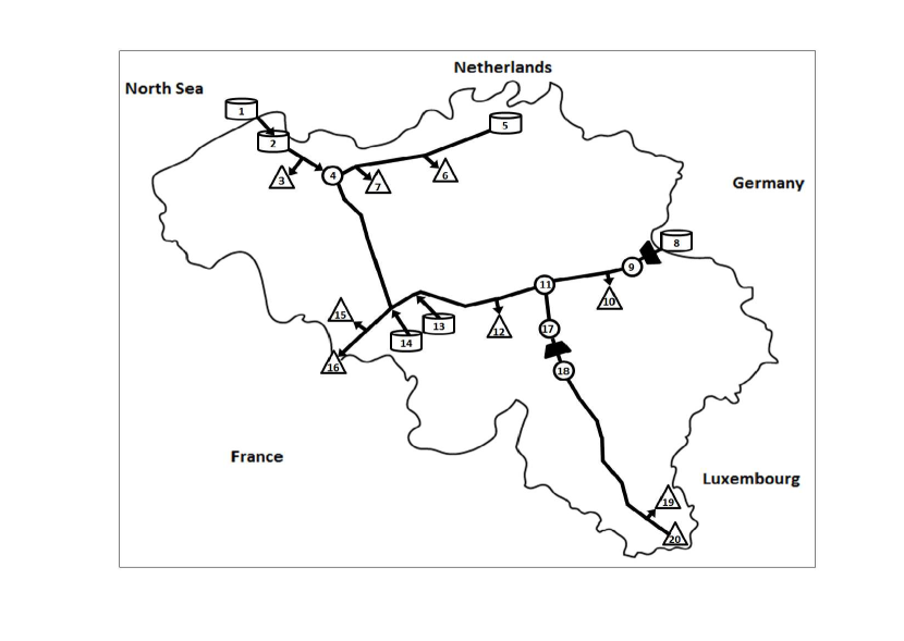
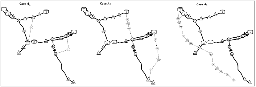
Table 1 shows the list of test instances based on the Belgian network depicted in Figure 2. The table shows, for each benchmark, the number of nodes, sources, terminals, base pipelines, and compressor stations, as well as the number of new components (pipelines and compressors) that can potentially be added to the network topology. Note that benchmark $A$ in Table 1 is the real Belgium gas transmission network and Table 3 shows the node characteristics for this 20-node, 24-pipeline, 3-compressor network. The reader is referred to the appendix of (De Wolf and Smeers 2000) for further details on this network. Instances $A_{1}-A_{3}$ captures various possible expansions to this base network. Figure 3 and Tables 5 and 6 depict the location of the potential expansion plans and their associated data. The network expansion plans were designed for the Belgian gas network in order to capture events such as increase of the number of nominations and forecasting demand at the city gates, as well as excessive stress of the available supplies at the sources.

Figure 2: The Belgian Gas Network Base Configuration (case $A$).

		Network configuration
					Base			New
Ref		$|{\cal N}|$	$|{\cal I}|$	$|{\cal D}|$	$|{\cal P}_{e}|$	$|{\cal C}_{e}|$		$|{\cal P}_{n}|$	$|{\cal C}_{n}|$
$A$		20	6	9	24	3		0	0
$A_{1}$		22	6	9	24	3		4	2
$A_{2}$		25	6	9	24	3		7	4
$A_{3}$		29	6	9	24	3		12	5
$B_{1}$		20	6	9	0	0		135	12
$B_{2}$		20	6	9	0	0		135	12
$B_{3}$		20	6	9	0	0		135	12
$B_{4}$		20	6	9	0	0		135	12

Table 1: Test Instances Based on the Belgian Network.

Instances $B_{1}-B_{4}$ are based on the “optimization from scratch” benchmarks from (De Wolf and Smeers 2000) and (Babonneau et al. 2012) ($\alpha=1,1.6,5,and6$, respectively). In these papers, the authors use the Belgian gas network for a variation of the GTNEP problem which considers integrated functions of the gas merchant and transportation process. These benchmarks specify minimum and maximum production levels (see Table 4). Since the GTNEP assumes known gas nomination and production profiles, we computed load and compression profiles based on optimal pressures provided in (Babonneau et al. 2012). Our instances also employ the same cost function as in (Babonneau et al. 2012) to compute the associated costs for building new pipelines, i.e.,

$$L_{ij}\left(1.04081^{-6}D_{ij}^{2.5}+11.2155\right)$$

where $D_{ij}$ and $L_{ij}$ are the diameter and length of pipeline $(i,j)$ respectively. (Babonneau et al. 2012) assumed continuous diameter choices. However, we used a discrete diameter values corresponding to the solution of (De Wolf and Smeers 2000) and Table 4 of (Babonneau et al. 2012). For completeness, the diameter choices are described in Table 2. Note that the exclusive-set constraint is slightly different for these cases due to the existence of pre-defined parallel pipes. Within in each row of Table 2, the solution must contain one and only diameter choice, and each set of parallel pipes must choose diameters from the same column of Table 2.

Pipe	$D_{1}$	$D_{2}$	$D_{3}$	$D_{4}$	$D_{5}$
(1,2) A	890.0	650.3	610.8	524.7	512.1
(1,2) B	890.0	650.3	610.8	524.7	512.1
(2,3) A	890.0	834.7	784.0	673.5	657.3
(2,3) B	890.0	834.7	784.0	673.5	657.3
(3,4)	890.0	998.9	938.3	806.0	786.7
(5,6)	590.1	604.3	567.6	487.6	475.9
(6,7)	590.1	0	X	X	X
(7,4)	590.1	671.7	630.9	542.0	529.0
(4,14)	890.0	829.9	779.5	669.7	653.6
(8,9) A	890.0	902.8	848.0	728.4	711.0
(8,9) B	395.5	902.8	848.0	728.4	711.0
(9,10) A	890.0	902.8	848.0	728.4	710.9
(9,10) B	395.5	902.8	848.0	728.4	711.0
(10.11) A	890.0	787.6	739.8	635.5	620.1
(10.11) B	395.5	787.6	739.8	635.5	620.4
(11,12)	890.0	979.8	920.3	790.6	771.6
(12,13)	890.0	915.1	859.6	738.4	720.7
(13,14)	890.0	952.6	894.7	768.6	750.1
(14,15)	890.0	1201.0	1128.0	969.0	945.8
(15,16)	890.0	1038.4	975.3	837.9	817.7
(11,17)	395.5	469.0	440.5	378.4	369.3
(17,18)	315.5	469.0	440.5	378.4	369.3
(18,19)	315.5	469.0	440.5	378.4	369.3
(19,20)	315.5	448.9	421.7	362.2	353.5

Table 2: Pipe diameter choices from Table 4 of (Babonneau et al. 2012)

			(Loads)				(Pressure)
Node (Loc.)	Type(∗)		$\underline{L}$	$\overline{L}$	L		$\underline{P}$	$\overline{P}$
1 (Zeebrugge)	${\cal I}$		8.87	11.594	10.911288		0	77
2 (Dudzele)	${\cal I}$		0	8.4	8.4		0	77
3 (Brugge)	${\cal D}$		$-\infty$	-3.918	-3.918		30	80
4 (Zomergem)			0	0	0		0	80
5 (Loenhout)	${\cal I}$		0	4.8	2.814712		0	77
6 (Antwerp)	${\cal D}$		-$\infty$	-4.034	-4.034		30	80
7 (Ghent)	${\cal D}$		-$\infty$	-5.256	-5.256		30	80
8 (Voeren)	${\cal I}$		20.34	22.01	22.012		50	66.2
9 (Berneau)			0	0	0		0	66.2†
10 (Liège)	${\cal D}$		-$\infty$	-6.365	-6.365		30	66.2
11 (Warnand)			0	0	0		0	66.2
12 (Namur)	${\cal D}$		-$\infty$	-2.12	-2.12		0	66.2
13 (Anderlues)	${\cal I}$		0	1.2	1.2		0	66.2
14 (Péronnes)	${\cal I}$		0	0.96	0.96		0	66.2
15 (Mons)	${\cal D}$		-$\infty$	-6.848	-6.848		0	66.2
16 (Blaregnies)	${\cal D}$		-$\infty$	-15.616	-15.616		50	66.2
17 (Wanze)			0	0	0		0	66.2
18 (Sinsin)			0	0	0		0	63
19 (Arlon)	${\cal D}$		-$\infty$	-0.222	-0.222		0	66.2
20 (Pétange)	${\cal D}$		-$\infty$	-1.919	-1.919		25	66.2

Table 3: The Belgian Gas Network Data from  (De Wolf and Smeers 2000). This data is used for the A Problems. $\dagger$- On Problems A1, A2, and A3,the pressure bounds are $[0,59.851968]$, $[0,59]$, and $[0,59.85]$ respectively.

		Load ($L$) profiles (MMscf)
Node		$\;\;\;\;B_{1}$	$\;\;\;\;B_{2}$	$\;\;\;\;B_{3}$	$\;\;\;\;B_{4}$
1		9.5883	9.8225	9.8218	9.7205
2		8.1833	8.3447	8.1340	8.3628
3		-3.9180	-3.9180	-3.9180	-3.9180
4		0.0000	0.0000	0.0000	0.0000
5		4.0315	4.0432	4.0383	4.0364
6		-4.0315	-4.0432	-4.0383	-4.0364
7		-5.2413	-5.2644	-5.2562	-5.2644
8		22.012	22.0120	22.0120	22.0120
9		0.0000	0.0000	0.0000	0.0000
10		-6.4744	-6.4951	-6.3970	-6.3816
11		0.0000	0.0000	0.0000	0.0000
12		-2.1929	-2.1191	-2.1162	-2.0984
13		1.2162	1.3225	1.0802	1.1591
14		0.9840	0.6164	1.0776	1.0235
15		-6.4056	-6.5885	-6.8366	-6.8857
16		-15.6119	-15.5904	-15.4616	-15.5899
17		0.0000	0.0000	0.0000	0.0000
18		0.0000	0.0000	0.0000	0.0000
19		-0.2059	-0.2312	-0.2269	-0.2164
20		-1.9337	-1.9112	-1.9131	-1.9236

Table 4: The Load Profiles Computed from Optimal Pressures Provided in (Babonneau et al. 2012). All compression ratios were derived as 1.0.

Figure 3: The Belgian Gas Network Expansion Plans (Instances $A_{1}$–$A_{3}$).

Node		Town	Lat.	Long.	$\underline{P}^{(*)}$	$\overline{P}^{(*)}$
		Instance $A_{1}$
21		Bois	50.400676	5.855991	14	66
22		Koninklijke	50.806672	4.481877	14	66
		Instance $A_{2}$
21		Heist	51.095651	4.744616	20	70
22		Zoutleeuw	50.858734	5.115404	20	70
23		Beaufays	50.552195	5.670182	20	70
24		Gouvy	50.231757	5.966813	20	70
25		Ettelbruck	49.861370	6.073930	20	70
		Instance $A_{3}$
21		Jabbeke	51.204699	3.086440	14	66
22		Torhout	51.072867	3.118026	14	66
23		Kortrijk	50.790711	3.230636	14	66
24		Bois-de-Barry	50.580151	3.521773	14	66
25		Lobbes	50.353208	4.263261	20	70
26		Senzeille	50.124840	4.433550	20	70
27		Gedinne	49.980230	4.851030	20	70
28		Chiny	49.806832	5.274004	20	70
29		Pigneule	49.735878	5.471758	20	70

Table 5: Locations of Nodes of the Expansion Plans for the Belgian Gas Network. These nodes do not have injections.

Node	Node		$w$	$c$
Instance $A_{1}$
9	21		0.929	67.19
21	18		0.808	77.26
6	22		0.785	79.50
22	14		0.766	81.44
Instance $A_{2}$
5	21		1.052	59.29
21	$21^{*}$		Compressor	1500.0
22	11		0.967	64.52
8	23		1.933	32.28
23	24		0.876	71.18
24	$24^{*}$		Compressor	1500.0
25	19		1.339	46.59
$21^{*}$	22		0.980	63.65
$24^{*}$	25		0.866	72.08
Instance $A_{3}$
1	21		2.257	27.65
2	21		4.546	13.73
21	$21^{*}$		Compressor	1500.0
22	23		1.121	55.66
23	$23^{*}$		Compressor	1500.0
24	15		1.073	58.14
15	25		1.483	42.09
25	26		1.289	48.40
26	$26^{*}$		Compressor	1500.0
27	28		1.010	61.79
28	29		2.232	27.96
29	19		1.423	42.09
$21^{*}$	22		2.448	25.50
$23^{*}$	24		1.165	53.56
$26^{*}$	27		1.071	58.28

Table 6: Locations of Pipes of the Expansion Plans for the Belgian Gas Network. * denotes introduced dummy node for 0 length compressor arcs.

5.1.2 Larger Networks

Table 7 describes the main data points for the larger benchmarks. Instance $D$ is a real-life network case whose data is restricted for confidentiality reasons and we are not allowed to disclose its map or load profile. Instances $E,F$ and $G$ are part of a German network whose data, including the network configuration, maps, and load profiles, can be found in (Pfetsch et al. 2012).

		Network configuration
					Base			New
Ref.		$|{\cal N}|$	$|{\cal I}|$	$|{\cal D}|$	$|{\cal P}_{e}|$	$|{\cal C}_{e}|$		$|{\cal P}_{n}|$
$D$		60	2	24	55	4		55
$E$		40	3	29	39	6		39
$F$		135	6	99	141	29		141
$G$		582	31	129	609	5		278

Table 7: Larger Instances of Gas Networks.

5.2 The Algorithms and the Experimental Setting

This section reports computational results for three approaches:

1. The MINLP formulation of the GTNEP as shown in Model 2;

2. The MISOCP relaxation of the GTNEP as shown in Model 3 followed by the conversion presented in Section 4.4;

3. A MIP formulation based on a Piecewise Linear Approximation (PLA-MIP) of the quadratic functions; The PLA-MIP formulation follows the derivation in (Correa-Posada and Sánchez-Martín 2014, De Wolf and Smeers 2000) and uses 60 segments.

All the experiments weere conducted on a computer with two Intel Xeon CPU X5670 processors (2.93GHz) with 6 cores each. The computer has 64 GB DIMM 1333MHz RAM and runs the Ubuntu 14.04 LTS operating system. The MINLP formulation is solved using SCIP 3.1.1 (Achterberg 2009) compiled with Ipopt 3.12.3 and Cplex 12.6. The PLA-MIP formulation is solved using CPLEX 12.6 (ILOG CPLEX Optimization Studio 2013). The MISCOP formulation is solved with CPLEX 12.6 and the conversion is performed by IPOPT 3.12.3 (Wächter and Biegler 2006).

5.3 Results on the Belgian Network

Table 8 shows the sizes of the underlying models in terms of the number of binary and continuous variables and the number of linear and quadratic constraints for each instance. Table 9 presents the computational results and reports the CPU time in seconds and the upgrade cost in $\$\times 10^{3}$ for each approach. The computational results show that the MISOCP approach outperforms both the MINLP and the PLA-MIP and that the solution to the MISOCP always converts to a feasible and optimal solution. The PLA-MIP approach has both computational and accuracy issues, as it significantly underestimates the optimal objective value and is rather slow.

The results for problems B1–B4 are interesting as the expansion costs are considerably lower than reported by Babonneau et al. (2012) for the same operating conditions. In Table 4 of their paper, Babonneau et al. (2012) report expansion costs of 15669, 14252, 11610, and 11274 for B1–B4. Their solutions are feasible and have the same operating cost as our model. Of course, it is important to note than their solutions were obtained through a model that minimizes operating and expansion costs, which could make it harder to determine the best design for particular operating conditions. Still, this comparison highlights the strengths of the formulation proposed in this paper.

		MINLP						PLA-MIP						MISOCP
Bench.		BV	CV		LC	QC		BV	CV		LC	QC		BV	CV		LC	QC
$A$		54	49		254	96		1494	1837		3931	0		54	73		398	24
$A_{1}$		70	59		320	112		1750	2151		4605	0		66	91		488	28
$A_{2}$		85	69		389	124		1945	2391		5120	0		78	107		575	31
$A_{3}$		103	80		463	144		2263	2776		5954	0		91	128		679	36
$B_{1,2,3,4}$		354	1154		464	357		7314	8737		19067	0		238	373		1850	116

Table 8: The Sizes of the Mathematical models for Belgian Network Instances. (BV: Binary variables, CV: Continuous variables, LC: Linear constraints, QC: Quadratic constraints).

		MINLP			PLA-MIP			MISOCP
Bench.		CPU	Obj		CPU	Obj		CPU	Obj
$A$		0.02	0.0		0.6	0.0		0.03	0.0
$A_{1}$		0.06	144		0.7	144		0.05	144
$A_{2}$		0.06	1687		1.4	187		0.1	1687
$A_{3}$		0.06	1780		1.9	280		0.06	1780
$B_{1}$		1.89	11181		1089	10353		0.3	11181
$B_{2}$		3.17	11181		1781	10361		0.6	11181
$B_{3}$		3.53	11181		1538	10352		0.6	11181
$B_{4}$		3.82	11181		1570	10352		0.3	11181

Table 9: Computational Results on the Belgian Network Instances: The Objective Value is in $\$$ and the CPU Time in Seconds.

5.4 Scalability Results

We now study whether the results on the Belgian networks continue to hold on larger instances. To assess scalability and robustness, we stress the networks by gradually increasing the production and consumption levels from 5% up to 300% while considering solely the addition of a parallel pipe for each existing pipeline in the base configuration of the gas systems (i.e., $|{\cal C}_{n}|=0$). Table 8 presents the sizes of the mathematical models. In all of these results, we denote whether or not the MISOCP and MINLP solutions are exact, lower bounds, or upper bounds on the MINLP solutions. Lower bounds for the MINLP are also derived by subtracting the optimality gap from any primal feasible solution.

Table 11 presents the computational results on instance D which is based on proprietary natural gas network in the United States. Observe that the PLA-MIP model systematically underestimates the objective function and returns infeasible solutions. As we will see, this is systematic on all larger benchmarks. The MISOP approach returns optimal solutions for all but one case. Both the MINLP and MISOCP prove infeasibility of the most stressed network.

Table 12 presents the computational results on instance E which is based on gaslib-40 (GasLib 2014). The MISOP approach returns optimal solutions, or proves infeasibilities in all cases. The MISOP model is one order of magnitude faster than the MINLP model.

Table 13 presents the computational results on instance F, which is based on gaslib-135 (GasLib 2014) and is particularly challenging. The MINLP approach finds optimal solutions up to the 25% case and spends considerable time doing so. It finds an upper bound to the 50% case but does not return any information on the 75% and 100% cases. In contrast, the MISOCP approach finds optimal solutions to the 0%, 5%, 25%, and 50% cases, all below 10 seconds, It finds lower bounds on the 75% and 100% cases reasonably fast. Both the MINLP and the MISOCP prove infeasibility of the three most stressed instances.

Table 14 presents very interesting results for instance G, which is based on gaslib-582 (GasLib 2014). The MINLP approach cannot find feasible solutions on any of the cases but the 300% case which is shown infeasible. Both the MINLP and PLA-MIP approaches have numerical issues with these problems. The MISOP approach finds optimal solutions up to the 50% case and for the 150% case and proves infeasibilities for the 200% and 300% cases. For the 75%–125% cases, the MISCOP times out but returns upper bounds to the optimal solution with duality gaps ranging from 7.65% to 51.3%.

Overall, these results demonstrate the benefits of the MISOCP approach. The MISOCP approach almost always finds optimal solutions much faster than the MINLP when both return optimal solutions. It also finds optimal solutions or proves infeasibility in many case for the larger benchmarks, while the MINLP approach does not return feasible solutions.

		MINLP						PLA-MIP						MISOCP)
Ref.		BV	CV		LC	QC		BV	CV		LC	QC		BV	CV		LC	QC
$D$		283	174		1093	440		6883	8330		18018	0		228	339		1753	110
$E$		207	124		792	312		4887	5920		12796	0		168	241		1260	78
$F$		763	446		2886	1128		17683	21430		46304	0		622	869		4578	282
$G$		2101	1469		8058	2256		35941	44433		92848	0		1823	2311		11442	564

Table 10: Size of the Mathematical Models: BV: Binary variables, CV: Continuous variables, LC: Linear constraints, QC: Quadratic constraints.

Stresss		MINLP			PLA-MIP			MISOCP
level		CPU	Obj		CPU	Obj		CPU	Obj
0%		0.1	0.00★		3.0	0.00		0.1	0.00★
5%		0.5	3.50★		1.8	0.00		0.6	3.50★
10%		1.6	23.83★		12.2	23.22		0.5	23.83★
25%		2.1	92.24★		14.0	83.99		0.6	92.24★
50%		1.5	145.58★		14.8	136.2		0.5	145.58★
75%		0.6	191.80★		11.0	184.0		0.6	191.8★
100%		3.0	287.00★		12.5	209.03		0.7	281.99$\bigtriangleup$
125%		0.2	$\dagger\;\;\;\;$		1.6	$\dagger\;\;\;\;$		0.2	$\dagger\;\;\;\;$

Table 11: Computational Results on Instance D. Obj: $\$\times 10^{6}$, CPU time: in seconds, Solution status: ^★ = Proven optimal; $\bigtriangleup$ = Lower bound; $\bigtriangledown$ = Upper bound; $\dagger$ = Infeasible; $\ddagger$ = Unknown.

Stress		MINLP				PLA-MIP				MISOCP
level		CPU	Obj	Gap		CPU	Obj	Gap		CPU	Obj	Gap
0%		1.6	0.00★	0.0		10.2	0.00	0.0		0.2	0.00★	0.0
5%		6.3	11.92★	0.0		23.5	0.00	0.0		0.7	11.92★	0.0
10%		6.8	32.83★	0.0		20.6	0.00	0.0		0.4	32.83★	0.0
25%		5.6	41.08★	0.0		30.9	32.8	0.0		0.6	41.08★	0.0
50%		8.1	156.06★	0.0		11.5	32.8	0.0		0.9	156.06★	0.0
75%		12.0	333.01★	0.0		21.8	121.1	0.0		0.7	333.00★	0.0
100%		12.1	551.64★	0.0		17.5	122.37	0.0		0.8	551.64★	0.0
125%		2.2	$\dagger$	–		33.0	256.22	0.0		0.4	$\dagger$	–
150%		0.8	$\dagger$	–		27.6	$\dagger$	–		0.3	$\dagger$	–

Table 12: Computational Results on Instance E. Obj: $\$\times 10^{6}$, CPU time: in seconds, Solution status: ^★ = Proven optimal; $\bigtriangleup$ = Lower bound; $\bigtriangledown$ = Upper bound; $\dagger$ = Infeasible; $\ddagger$ = Unknown.

Stress		MINLP				PLA-MIP				MISOCP
level		CPU	Obj	Gap		CPU	Obj	Gap		CPU	Obj	Gap
0%		0.85	0.0★	0.0		136.3	0.0	0.0		1.3	0.0★	0.0
5%		101.8	0.0★	0.0		120.0	0.0	0.0		1.0	0.0★	0.0
10%		36707.3	15.04★	0.0		125.8	0.0	0.0		2.4	0.0$\bigtriangleup$	0.0
25%		457.9	60.4★	0.0		124.4	0.0	0.0		4.4	60.4★	0.0
50%		86962.9	182.7$\bigtriangledown$	91.7		166.7	60.4	0.0		7.6	95.3★	0.0
75%		86933.9	$\ddagger$	–		119.8	60.4	0.0		40.5	451.5$\bigtriangleup$	0.0
100%		87334.2	$\ddagger$	–		119.5	149.6	0.0		104.6	1234.2$\bigtriangleup$	0.0
125%		6.8	$\dagger$	–		125.7	149.6	0.0		1.8	$\dagger$	0.0
150%		3.4	$\dagger$	–		206.7	486.0	0.0		1.1	$\dagger$	0.0
200%		0.4	$\dagger$	–		11.6	$\dagger$	–		0.4	$\dagger$	0.0

Table 13: Computational Results on Instance F. Obj: $\$\times 10^{6}$, CPU time: in seconds, Solution status: ^★ = Proven optimal; $\bigtriangleup$ = Lower bound; $\bigtriangledown$ = Upper bound; $\dagger$ = Infeasible; $\ddagger$ = Unknown.

Stress		MINLP				PLA-MIP				MISOCP
level		CPU	Obj	Gap		CPU	Obj	Gap		CPU	Obj	Gap
0%		86400.0	$\ddagger$	–		62012.9	6.87	0.0		2.7	0.00★	0.0
5%		86400.0	$\ddagger$	–		29655.1	2.78	0.0		4.4	0.00★	0.0
10%		86400.0	$\ddagger$	–		86400.0	4.65	40.22		21.1	0.00★	0.0
25%		86400.0	$\ddagger$	–		2153.2	8.65	0.0		40.9	0.00★	0.0
50%		86400.0	$\ddagger$	–		3670.2	$\dagger$	–		164.0	14.93★	0.0
75%		86400.0	$\ddagger$	–		0.21	$\dagger$	–		86402.1	111.99$\bigtriangledown$	51.3
100%		86400.0	$\ddagger$	–		5.31	$\dagger$	–		86401.6	332.53$\bigtriangledown$	7.65
125%		86400.0	$\ddagger$	–		5.31	$\dagger$	–		86402.4	524.82$\bigtriangledown$	11.74
150%		86400.0	$\ddagger$	–		5.29	$\dagger$	–		53321.3	590.84★	0.0
200%		86400.0	$\ddagger$	–		5.02	$\dagger$	–		16.7	$\dagger$	–
300%		4.4	$\dagger$	–		0.12	$\dagger$	–		0.9	$\dagger$	–

Table 14: Computational Results on Instance G. Obj: $\$\times 10^{6}$, CPU time: in seconds, Solution status: ^★ = Proven optimal; $\bigtriangleup$ = Lower bound; $\bigtriangledown$ = Upper bound; $\dagger$ = Infeasible; $\ddagger$ = Unknown.

5.5 The Importance of Integer Cuts

Table 15 describes the performance of the MISCOP on instances E, F, and G when the integer cuts are not used. As can be seen, the integer cuts, which were used both in the MINLP and MISOCP models, are critical to obtain an efficient MISOCP implementation.

Stress		Instance $E$				Instance $F$				Instance $G$
level		CPU	Obj	Gap		CPU	Obj	Gap		CPU	Obj	Gap
0%		0.9	0.00★	0.0		3310.9	0.00★	0.0		242.2	0.00★	0.0
5%		1.8	11.92★	0.0		83.5	0.00★	0.0		14.2	0.00★	0.0
10%		2.7	32.83★	0.0		120.7	0.00$\bigtriangleup$	0.0		301.5	0.00★	0.0
25%		3.2	41.08★	0.0		86419.5	60.44$\bigtriangledown$	75.1		86400.3	$\ddagger$	–
50%		8.5	156.06★	0.0		17693.1	95.32$\bigstar$	0.0		8271.05	14.93★	0.0
75%		6.7	333.01★	0.0		86409.9	451.59	59.2		86404.4	111.99$\bigtriangledown$	79.4
100%		3.8	551.64★	0.0		86404.5	1234.23	44.2		87193.1	332.32$\bigtriangledown$	87.9
125%		1.8	$\dagger$	–		90.9	$\dagger$	–		86401.8	524.82$\bigtriangledown$	16.1
150%		1.0	$\dagger$	–		7.5	$\dagger$	–		86408.9	245.80$\bigtriangleup$	58.5
200%		0.7	$\dagger$	–		2.0	$\dagger$	–		13318.6	$\dagger$	–
300%		0.0	$\dagger$	–		0.0	$\dagger$	–		3.0	$\dagger$	–

Table 15: Computational Results on Instances E, F, and G without the Integer Cuts. Obj: $\$\times 10^{6}$, CPU time: in seconds, Solution status: ^★ = Proven optimal; $\bigtriangleup$ = Lower bound; $\bigtriangledown$ = Upper bound; $\dagger$ = Infeasible; $\ddagger$ = Unknown

6 Concluding Remarks

This paper considered the expansion of natural gas networks, a critical process involving substantial capital expenditures with complex decision-support requirements. It proposed a convex mixed-integer second-order cone relaxation for the gas expansion planning problem under steady-state conditions in order to address the fact that state-of-the-art global optimisation solvers are unable to scale up to real-world size instances. The resulting MISOCP model offers tight lower bounds with high computational efficiency. In addition, the optimal solution of the relaxation can often be used to derive high-quality solutions to the original problem, leading to provably tight optimality gaps and, in some cases, global optimal solutions. The convex relaxation is based on a few key ideas, including the introduction of flux direction variables, exact McCormick relaxations, on/off constraints, and integer cuts. Numerical experiments are conducted on the traditional Belgian gas network, as well as other real larger networks. The computational results demonstrate that the MISOCP model is faster than the originating MINLP model by one or two orders of magnitude on the Belgian network instances. They also show that the MISOCP model scales well to large and stressed instances.

References

- Achterberg (2009) Achterberg, T. 2009. Scip: Solving constraint integer programs. Mathematical Programming Computation 1 1–41.
- André (2010) André, J. 2010. Optimization of investments in gas networks. Phd thesis, School in Business, Université Lille Nord de France, France.
- Andre et al. (2009) Andre, J., F. Bonnans, L. Cornibert. 2009. Optimization of capacity expansion planning for gas transportation networks. European Journal of Operational Research 197 1019–1027.
- Atamturk (2002) Atamturk, A. 2002. On capacitated network design cut-set polyhedra. Math. Programming 92 425–437.
- Babonneau et al. (2009) Babonneau, F., Y. Nesterov, J.-P. Vial. 2009. Design and operations of gas transmission networks.
- Babonneau et al. (2012) Babonneau, F., Y. Nesterov, J.-P. Vial. 2012. Design and operations of gas transmission networks. Operations Research 60 34–47.
- Bakhouya and De Wolf (2008) Bakhouya, B., D. De Wolf. 2008. Optimal dimensioning of pipe networks: the new situation when the distribution and the transportation functions are disconnected. In: 22th Conference on Quantitative Methods for Decision Making.
- Bonami and Lee (2013) Bonami, P., J. Lee. 2013. Bonmin – user’s manual.
- Bonnans et al. (2011) Bonnans, J.F., G. Spiers, J.-L. Vie. 2011. Global optimization of pipe networks by the interval analysis approach: The Belgium network case. Tech. rep., Inria Research Report RR-7796, November.
- Boyd et al. (1994) Boyd, I.D., P.D. Surry, N.J. Radcliffe. 1994. Constrained gas network pipe sizing with genetic algorithms.
- Coelho and Pinho (2007) Coelho, P.M., C. Pinho. 2007. Considerations about equations for steady state flow in natural gas pipelines. J. of the Braz. Soc. of Mech. Sci. & Eng XXIX 262–273.
- Correa-Posada and Sánchez-Martín (2014) Correa-Posada, C.M., P. Sánchez-Martín. 2014. Security-constrained optimal power and natural-gas flow. IEEE Transactions on Power Systems 29 1780–1787.
- De Wolf et al. (1991) De Wolf, D., O. Janssens de Bisthoven, Y. Smeers. 1991. The simplex algorithm extended to piecewise linearly constrained problems i: the method and an implementation. Tech. rep., Université Catholique de Louvain, Louvain, Belgium.
- De Wolf and Smeers (1996) De Wolf, D., Y. Smeers. 1996. Optimal dimensioning of pipe networks with application to gas transmission networks. Operations Research 44 596–608.
- De Wolf and Smeers (2000) De Wolf, D., Y. Smeers. 2000. The gas transmission problem solved by an extension of the simplex algorithm. Management Science 46 1454–1465.
- Edgar et al. (1978) Edgar, T.F, D.M Himmelblau, T.C. Bickel. 1978. Optimal design of gas transmission network. Society of Petroleum Engineers Journal 96–104.
- Edgar et al. (2001a) Edgar, T.F., D.M. Himmelblau, L.S. Lasdon. 2001a. http://www.gams.com/modlib/libhtml/gasnet.htm.
- Edgar et al. (2001b) Edgar, T.F., D.M. Himmelblau, L.S. Lasdon. 2001b. Optimization of Chemical Processes. Chapter 9: Mixed-Integer Programming. 2nd Edition, McGraw-Hill, Boston.
- Elshiekh et al. (2013) Elshiekh, T.M., S.A. Khalil, H.A. El Mawgoud. 2013. Optimal design and operation of egyptian gas-transmission pipelines. Oil and Gas Facilities, Society of Petroleum Engineers 44–48.
- GAMS Development Corporation (2008) GAMS Development Corporation. 2008. GAMS: The Solver Manuals.
- GasLib (2014) GasLib. 2014. Gaslib: A library of gas network instances.
- Hansen et al. (1991) Hansen, C.T., K. Madsen, H.B. Nielsen. 1991. Optimization of pipe networks. Mathematical Programming 52 45–58.
- Hijazi et al. (2010) Hijazi, H., P. Bonami, G. Cornuéjols, A. Ouorou. 2010. Mixed integer nonlinear programs featuring âon/offâ constraints: convex analysis and applications. Electronic notes in Discrete Mathematics 36 1153–1160. doi:10.1016/j.endm.2010.05.146.
- Hijazi et al. (2012) Hijazi, H., P. Bonami, G. Cornuéjols, A. Ouorou. 2012. Mixed-integer nonlinear programs featuring âon/offâ constraints. Computational Optimization and Applications 52 537–558. 10.1007/s10589-011-9424-0. URL http://dx.doi.org/10.1007/s10589-011-9424-0.
- Humpola and Fügenschuh (2014a) Humpola, J., A. Fügenschuh. 2014a. A new class of valid inequalities for nonlinear network design problems. Angewandte Mathematik und Optimierung Schriftenreihe (AMOS#4), Applied Mathematics and Optimization Series .
- Humpola and Fügenschuh (2014b) Humpola, J., A. Fügenschuh. 2014b. A unified view on relaxations for a nonlinear network flow problem. Angewandte Mathematik und Optimierung Schriftenreihe (AMOS#6), Applied Mathematics and Optimization Series .
- Humpola and Fügenschuh (2015) Humpola, J., A. Fügenschuh. 2015. Convex reformulations for solving a nonlinear network design problem. Comput Optim Appl .
- Humpola et al. (2015a) Humpola, J., A. Fügenschuh, T. Koch. 2015a. Valid inequalities for the topology optimization problem in gas network design. OR Spectrum .
- Humpola et al. (2015) Humpola, J., A. Fügenschuh, T. Lehmann. 2015. A primal heuristic for optimizing the topology of gas networks based on dual information. EURO J Comput Optim 3 53–78.
- ILOG CPLEX Optimization Studio (2013) ILOG CPLEX Optimization Studio, IBM. 2013. Cplex userâs manual, version 12 release 6.
- LINDO Systems (1997) LINDO Systems. 1997. Lingo 3.1 modeling software.
- Markowitz and Manne (1957) Markowitz, H.M., A. Manne. 1957. On the solution of discrete programming problems. Econometrica 25 84–110.
- U.S. Energy Information Administration (2008) U.S. Energy Information Administration. 2008. http://www.eia.gov/pub/oil_gas/natural_gas/analysis_ publications/ngpipeline/develop.html.
- McCormick (1976) McCormick, G.P. 1976. Computability of global solutions to factorable nonconvex programs, part i: convex underestimating problems. Mathematical Programming 10 147–175.
- Murtagh and Saunders (1998) Murtagh, B.A., M.A. Saunders. 1998. Minos 5.5 users guide. Tech. rep., Department of Operations Research, Stanford University, California.
- O’Neill et al. (1979) O’Neill, R.P., M. Williard, B. Wilkins, R. Pike. 1979. A mathematical programming model for allocation of natural gas. Operations Research 27 857–873.
- Osiadacz (1987) Osiadacz, A. 1987. Simulation and analysis of gas networks. Gulf Pub. Co. URL http://books.google.com/books?id=cMxTAAAAMAAJ.
- Pfetsch et al. (2012) Pfetsch, M.E., A. Fügenschuh, B. Geißler, N. Geißler, R. Gollmer, B. Hiller, J. Humpola, T. Koch, T. Lehmann, A. Martin, A. Morsi, J. Rövekamp, L. Schewe, M. Schmidt, R. Schultz, R. Schwarz, J. Schweiger, C. Stangl, M.C. Steinbach, S. Vigerske, B.M. Willert. 2012. Validation of nominations in gas network optimization: Models, methods, and solutions.
- Poss (2011) Poss, M. 2011. Models and algorithms for network design problems. Phd thesis, Faculté des Sciences, Département d’Informatique,Université Libre de Bruxelles, Belgium.
- Sardanashvili (2005) Sardanashvili, S. A. 2005. Computational Techniques and Algorithms (Pipeline Gas Transmission) [in Russian]. FSUE Oil and Gaz, I.M. Gubkin, Russian State University of Oil and Gas.
- Soliman and Murtagh (1982) Soliman, F.I., B.A. Murtagh. 1982. The solution of large-scale gas pipeline design problems. Engineering Optimization 6 77–83.
- Thorley and Tiley (1987) Thorley, A.R.D., C.H. Tiley. 1987. Unsteady and transient flow of compressible fluids in pipelinesâa review of theoretical and some experimental studies. International Journal of Heat and Fluid Flow 8 3 – 15. http://dx.doi.org/10.1016/0142-727X(87)90044-0. URL http://www.sciencedirect.com/science/article/pii/0142727X87900440.
- Uster and Dilaveroglu (2014) Uster, H., S. Dilaveroglu. 2014. Optimization for design and operation of natural gas transmission networks. Applied Energy 133 56–69.
- Vajda (1964) Vajda, S. 1964. Mathematical Programming. Addison-Wesley.
- Wächter and Biegler (2006) Wächter, A., L.T. Biegler. 2006. On the implementation of an interior-point filter line-search algorithm for large-scale nonlinear programming. Mathematical Programming 106 25–57. 10.1007/s10107-004-0559-y. URL http://dx.doi.org/10.1007/s10107-004-0559-y.
- Wilson et al. (1988) Wilson, J.G., J. Wallace, B.P. Furey. 1988. Steady-state optimization of large gas transmission systems. In: Simulation and optimization of large systems (A.J. Osiadacz Ed). Clarendon Press, Oxford.
- Wolf (2004) Wolf, De. 2004. Mathematical properties of formulations of the gas transmission problem. SMG Preprint 94/12, Université Catholique de Louvain, Belgium .
- Zheng et al. (2010) Zheng, Q.P., S. Rebennack, N.A. Iliadis, P.M. Pardalos. 2010. Optimization models in the natural gas industry. In: Handbook of Power Systems I 121–148.